Abstract

We study a multi-objective pure exploration problem in a multi-armed bandit model. Each arm is associated to an unknown multi-variate distribution and the goal is to identify the distributions whose mean is not uniformly worse than that of another distribution: the Pareto optimal set. We propose and analyze the first algorithms for the fixed budget Pareto Set Identification task. We propose Empirical Gap Elimination, a family of algorithms combining a careful estimation of the “hardness to classify” each arm in or out of the Pareto set with a generic elimination scheme. We prove that two particular instances, EGE-SR and EGE-SH, have a probability of error that decays exponentially fast with the budget, with an exponent supported by an information theoretic lower-bound. We complement these findings with an empirical study using real-world and synthetic datasets, which showcase the good performance of our algorithms.

1 INTRODUCTION

The multi-armed bandit problem has been extensively studied in the literature, predominantly as a single-objective stochastic optimization problem. In this framework, an agent sequentially collects samples from a set of $K$ (unknown) probability distributions, called arms. Two common goals are either to maximize the sum of observations (regret minimization, (Lattimore and CSzepesvári,, 2020)) or to identify the arm with the largest expected value (best arm identification, Even-Dar et al., (2002); Audibert and Bubeck, (2010)). In many real-world problems, however, there are multiple (possibly conflicting) objectives to optimize simultaneously and there might not exist a unique arm that maximizes all these objectives. This leads to a scenario in which the observations are multi-dimensional, and there may be several Pareto optimal arms. An arm belongs to the Pareto optimal set $\mathcal{S}^{\star}$ if it is not dominated by any other arm (in the sense that the mean values of all the objectives would be larger for the latter). While some line of work aims at minimizing the Pareto regret by strategically selecting arms from the Pareto set along the agent’s trajectory (Drugan and Nowe,, 2013), we are interested in the pure exploration counterpart of this problem, first studied by Auer et al., (2016), in which the goal is to identify (relaxations of) the set $\mathcal{S}^{\star}$, as quickly and accurately as possible. This multi-objective exploration problem has a wide range of applications including adaptive clinical trials (with multiple indicators of efficacy), software and hardware design (with multiple criteria such as speed and energy consumption), or A/B/n testing for recommender systems (with different metrics of users engagement).

Notably, prior work (Auer et al.,, 2016; Ararat and Tekin,, 2023; Kone et al.,, 2023) has studied the Pareto Set Identification (PSI) problem under the fixed-confidence setting: given a risk $\delta\in(0,1)$, the agent stops at a random time $\tau$ and recommends a set $\widehat{S}_{\tau}$ such that $\mathbb{P}(\widehat{S}_{\tau}\neq\mathcal{S}^{\star})\leq\delta$, while minimizing its expected stopping time $\mathbb{E}[\tau]$. However, to the best of our knowledge, no algorithms have been proposed for the dual fixed-budget setting in which the agent should output a guess for the Pareto set after a given budget $T$ while minimizing its probability of error $\mathbb{P}(\widehat{S}_{T}\neq\mathcal{S}^{\star})$. For some applications, the fixed-budget setting can be viewed as more practical: e.g., in clinical trials the maximal number of patients is typically defined in advance (due to some financial constraints), and the stopping time used in the fixed-confidence formulation could be prohibitively large.

We fill this gap by proposing the first algorithm(s) for Pareto Set Identification in the fixed-budget setting. Our approach may be viewed as an extension of Successive Rejects (SR) (Audibert and Bubeck,, 2010) and Sequential Halving (SH) (Karnin et al.,, 2013), two state-of-the-art algorithms for fixed-budget best arm identification (i.e. PSI in the uni-dimensional setting), that are based on arm eliminations. We propose a novel arm elimination criterion based on the computation of an Empirical Gap. This quantity can be viewed as a measure of the hardness to classify an arm as Pareto optimal or sub-optimal and is inspired by the gaps featured in the analysis of fixed-confidence algorithms (Auer et al.,, 2016; Kone et al.,, 2023). While SR and SH successively eliminate arms with smallest empirical means, in Empirical Gap Elimination (EGE), the arms with the largest empirical gaps are eliminated and appropriately classified as optimal or sub-optimal.

We prove an upper bound on the error probability of a generic version of EGE using any arm allocations satisfying some budget constraints (Theorem 1). We explicit our bound for two instances using the same arm allocations as SR and SH respectively, called EGE-SR and EGE-SH, showing that their error probability decrease exponentially fast with the budget (1.1). We derive an information-theoretic lower bound showing that these algorithms are essentially optimal in the worse case (Theorem 2). On the practical side, we report in Section 6 some experimental results showing that EGE-SR/SH outperform uniform sampling and are much more robust than APE-FB ​, an adaptation of an existing fixed-confidence algorithm that requires some prior knowledge of the problem complexity as input (discussed in Appendix D). Finally, we propose in Section 5, EGE-SR-$k$ ​, a variant of EGE-SR that tackles a relaxation of PSI first considered by Kone et al., (2023) in which one should identify at most $k$ Pareto optimal arms, with a provably reduced probability of error.

Related work

The Best Arm Identification problem (BAI) is one of the most studied pure exploration problems in the bandit literature. The fixed-confidence formulation of BAI is by now well understood as there are efficient algorithms with guaranteed bounds on their sample complexity, $\mathbb{E}[\tau]$ (e.g., (Kalyanakrishnan et al.,, 2012; Gabillon et al.,, 2012; Jamieson et al.,, 2014)) and some algorithms that attain the minimal sample complexity on any (parametric) problem instance in the asymptotic regime $\delta\rightarrow 0$ (e.g., (Garivier and Kaufmann,, 2016; You et al.,, 2023)). In contrast, the theoretical understanding of fixed-budget BAI is more elusive. While the error probability of any reasonable strategy (e.g. uniform sampling) decays exponentially fast with the budget $T$, Degenne, (2023) shows that there is no optimal exponent that can be attained by a single algorithm on all bandit instances. Still, the Successive Reject and Sequential Halving algorithms mentioned above have their error probability scaling in $\exp(-T/\log(K)H(\nu))$ for some complexity quantity $H(\nu)$ depending on the bandit instance $\nu$ and Carpentier and Locatelli, (2016) proved a (worse-case) lower bound showing that there exists instances $\nu$ in which this rate is un-improvable (up to constant factors in the exponent) when the budget $T$ is large.

In recent years, there has been a growing interest in pure exploration problems in a multi-dimensional setting. Adaptive algorithms for Pareto Set Identification were first proposed in the literature on black-box multi-objective optimization. Besides several evolutionary heuristics (e.g., Deb et al., (2002); Knowles, (2006)), the works of Zuluaga et al., (2013, 2016) have studied PSI under a Gaussian Process modeling assumption, obtaining some error bounds that decay polynomially in $T$ and depend on some notion of information gain that is specific to the GP setting. In the bandit literature, the first fixed-confidence PSI algorithm proposed by Auer et al., (2016) is based on uniform sampling and an accept/reject mechanism. Kone et al., (2023) then proposed a more adaptive LUCB-like algorithm for PSI and some relaxations introduced therein. Ararat and Tekin, (2023) studied an extension of PSI to any $\mathbb{R}^{D}$ partial order defined by an ordering cone, still in the fixed confidence setting.

Alongside PSI, other multi-dimensional pure exploration problems have been investigated such as feasible arm identification (Katz-Samuels and Scott,, 2018) in which the goal is to identify the arms which belong to a given polyhedron $\mathcal{P}\subset\mathbb{R}^{D}$ or top feasible arm identification (Katz-Samuels and Scott,, 2019) in which one seeks a feasible arm that further maximizes some linear combinations of the different objectives. While the former work considers the fixed-budget setting and also proposes some counterpart of Successive Rejects, the latter considers the fixed-confidence setting. In the fixed-budget setting, a special case was recently considered by Faizal and Nair, (2022) in a 2-dimensional setting in which the goal is to find the arm maximizing one attribute under the constraint that the second attribute is larger than a given threshold. They propose a SR like algorithm that is similar in spirit to our Empirical Gap Elimination, but with a very different notion of empirical gap.

2 SETTING

We formalize the fixed budget Pareto Set Identification problem and introduce some notation.

We are given $K$ distributions $\nu_{1},\dots,\nu_{K}$ over $\mathbb{R}^{D}$ with means (resp.) $\bm{\theta}_{1},\dots,\bm{\theta}_{K}$, called arms. Let $\nu:=(\nu_{1},\dots,\nu_{K})$ be the bandit instance and $\bm{\Theta}:=(\bm{\theta}_{1}\dots\bm{\theta}_{K})^{\intercal}$. We use Boldfaced symbols for $\mathbb{R}^{D}$ elements. As in prior work prior on multi-objective pure exploration, we assume that the marginal distributions of each arm are all $\sigma$-subgaussian. We recall that a random variable $X$ is $\sigma$-subgaussian if $\forall\;u\in\mathbb{R}$, $\mathbb{E}[\exp\left(u(X-\mathbb{E}[X])\right)]\leq\exp\left({u^{2}\sigma^{2}}/2\right)$.

Definition 1.

Given two arms $i,j\in[K]$, $i$ is weakly (Pareto) dominated by $j$ (denoted by $\bm{\theta}_{i}\leq\bm{\theta}_{j}$) if for any $d\in\{1,\dots,D\}$, $\theta_{i}^{d}\leq\theta_{j}^{d}$. The arm $i$ is (Pareto) dominated by $j$ ($\bm{\theta}_{i}\preceq\bm{\theta}_{j}$ or $i\prec j$) if $i$ is weakly dominated by $j$ and there exists $d\in\{1,\dots,D\}$ such that $\theta_{i}^{d}<\theta_{j}^{d}$. The arm $i$ is strictly (Pareto) dominated by $j$ ($\bm{\theta}_{i}\prec\bm{\theta}_{j}$ or $i\prec j$) if for any $d\in\{1,\dots,D\}$, $\theta_{i}^{d}<\theta_{j}^{d}$.

The Pareto set $\mathcal{S}^{\star}(\nu)$ is

$$\mathcal{S}^{\star}(\nu):=\left\{i\in[K]\textrm{ s.t }\nexists j\in[K]:\bm{\theta}_{i}\prec\bm{\theta}_{j}\right\},$$

and will be denoted by $\mathcal{S}^{\star}$ when $\nu$ is clear from the context. Any arm $a\in\mathcal{S}^{\star}$ will be called (Pareto) optimal and an arm $a\notin\mathcal{S}^{\star}$ is called sub-optimal.

At each time $t=1,2,\dots,T$, the agent chooses an arm $a_{t}$ and observes an independent draw $\mathbf{X}_{t}\sim\nu_{a_{t}}$ with $\mathbb{E}(\mathbf{X}_{a_{t}})=\bm{\theta}_{a_{t}}$. We denote by $\mathbb{P}_{\nu}$ the law of the stochastic process $\{\mathbf{X}_{t}\}_{t\geq 1}$ and by $\mathbb{E}_{\nu}$, the expectation under $\mathbb{P}_{\nu}$. Let $\mathcal{F}_{t}:=\sigma(a_{1},\mathbf{X}_{1},\dots,a_{t},\mathbf{X}_{t})$ be the $\sigma$-algebra representing the history of the process up to time $t$ and $\mathcal{F}:=\{\mathcal{F}_{t}\}_{t\geq 1}$, the filtration of the process. The agent’s strategy is adaptive in the sense that $a_{t}$ is $\mathcal{F}_{t-1}$ measurable. At time $T$, the agent outputs a guess $\widehat{S}_{T}$ (which is $\mathcal{F}_{T}$ measurable) for $\mathcal{S}^{\star}$ which should minimize the error probability $e_{T}(\nu):=\mathbb{P}_{\nu}(\widehat{S}_{T}\neq\mathcal{S}^{\star}(\nu))$.

To characterize the difficulty of the problem, we introduce below some quantities that allow to measure how much an arm is dominated. For any arms $i,j$, we let

$$\operatorname{m}(i,j) := \min_{d}\left[\theta_{j}^{d}-\theta_{i}^{d}\right],$$

$$\operatorname{M}(i,j) := \max_{d}\left[\theta_{i}^{d}-\theta_{j}^{d}\right].$$

If $\bm{\theta}_{i}\nprec\bm{\theta}_{j}$, $\operatorname{M}(i,j)$ is the smallest uniform increase of $j$ that makes it dominate $i$. If $\bm{\theta}_{i}\prec\bm{\theta}_{j}$ then $\operatorname{m}(i,j)$ is the smallest increase of any component of $i$ which makes it non-dominated by $j$. Auer et al., (2016) proposed an algorithm in the fixed-confidence setting whose sample complexity is characterized by some sub-optimality gaps $\Delta_{i}$’s defined as follows. For a sub-optimal arm $i\notin\mathcal{S}^{\star}$,

$$\Delta_{i}:=\Delta_{i}^{\star}:=\max_{j\in\mathcal{S}^{\star}}\operatorname{m}(i,j),$$ (1)

which is the smallest quantity that should be added component-wise to $\bm{\theta}_{i}$ to make $i$ appear Pareto optimal w.r.t $\{\bm{\theta}_{k}:k\in[K]\setminus\{i\}\}$. For an optimal arm $i\in\mathcal{S}^{\star}$,

$$\Delta_{i}:=\min(\delta_{i}^{+},\delta_{i}^{-})$$ (2)

where

$$\delta_{i}^{+} := \min_{j\in\mathcal{S}^{\star}\setminus\{i\}}\min(\operatorname{M}(i,j),\operatorname{M}(j,i))\;,$$

$$\delta_{i}^{-} := \min_{j\in[K]\setminus\mathcal{S}^{\star}}\{(\operatorname{M}(j,i))^{+}+\Delta_{j}\}\;,$$

with the convention $\min_{\emptyset}=+\infty$. $\delta_{i}^{+}$ accounts for how much $i$ is close to dominate (or to be dominated by) another optimal arm while $\delta_{i}^{-}$ translates in a sense the smallest “margin” from an optimal arm $i$ to the sub-optimal arms. Auer et al., (2016) show that the difficulty (i.e. near-optimal sample complexity) of fixed-confidence PSI is characterized by the complexity term

$$H(\nu):=\sum_{a=1}^{K}\frac{1}{\Delta_{a}^{2}}.$$

In this work, we show that it is also a relevant complexity measure for the fixed-budget setting.

3 ALGORITHMS

In this section, we introduce the family of Empirical Gap Elimination (EGE) algorithms.

3.1 Empirical Gap Elimination

An Empirical Gap Elimination algorithm uses a round-based structure. The algorithm is parameterized by a number of rounds $R>0$, an arm schedule vector $\bm{\lambda}=(\lambda_{1},\dots,\lambda_{R},\lambda_{R+1})\in[K]^{R+1}$ satisfying $\lambda_{r}>\lambda_{r+1}$ where $\lambda_{r}$ indicates how many arms are active in round $r$, and an allocation vector $\bm{t}=(t_{1},\dots,t_{R})\in[T]^{R}$, where $t_{r}$ is the number of samples gathered from each active arm in round $r$. Given the maximal budget $T$, these vectors should further satisfy the following:

$$\lambda_{1}=K\quad\text{and}\quad\lambda_{R+1}\in\{0,1\}$$ (3)

$$\text{and}\quad\sum_{r=1}^{R}\lambda_{r}t_{r}\leq T,$$ (4)

ideally with an equality.

In each round $r$, the algorithm maintains a set of active arm, denoted by $A_{r}$, that is of size $\lambda_{r}$, and collects $t_{r}$ new samples from each arm in $A_{r}$. The total number of samples from each arm in $A_{r}$ gathered in the first $r$ rounds is therefore

$$n_{r}=\sum_{s=1}^{r}t_{s}.$$

For each $a\in A_{r}$, the empirical estimate of $\bm{\theta}_{a}$ at the end of round $r$ is denoted by $\bm{\widehat{\theta}}_{a}(r):=\frac{1}{n_{r}}\sum_{s=1}^{n_{r}}\mathbf{X}_{a,s}$ where $\mathbf{X}_{a,s}$ denote the $s$-th observation drawn ​​​ i.i.d from distribution $\nu_{a}$. These estimates are used to carefully decide which arm to explore in the next round, based on an appropriate notion of empirical gap.

These gaps are empirical variants of the (fixed-confidence) gaps introduced in the previous section. We first propose a rewriting of these quantities to remove the explicit dependency on $\mathcal{S}^{\star}(\nu)$.

Lemma 1.

For any arm $i\in[K]$,

$$\Delta_{i}=\left\{\begin{array}[]{ll}\Delta_{i}^{\star}=\max_{j\in[K]}\operatorname{m}(i,j)&\text{ if }i\notin\mathcal{S}^{\star}\\ \delta_{i}^{\star}&\text{ if }i\in\mathcal{S}^{\star}\\ \end{array}\right.\;,$$

where $\delta_{i}^{\star}:=\min_{j\neq i}[\operatorname{M}(i,j)\land(\operatorname{M}(j,i)^{+}+(\Delta_{j}^{\star})^{+})].$

We introduce the empirical quantities

$$\operatorname{{{m}}}(i,j;r) := \min_{d}\left[{\widehat{\theta}}_{j}^{d}(r)-{\widehat{\theta}}_{i}^{d}(r)\right],$$

$$\operatorname{{{M}}}(i,j;r) := \max_{d}\left[({\widehat{\theta}}_{i}^{d}(r)-{\widehat{\theta}}_{j}^{d}(r))\right].$$

and the empirical Pareto set

$$S_{r} := \{i\in A_{r}:\nexists j\in A_{r}:\bm{\widehat{\theta}}_{i}(r)\prec\bm{\widehat{\theta}}_{j}(r)\},$$

$$= \{i\in A_{r}:\forall j\in A_{r}\backslash\{i\},\operatorname{{{M}}}(i,j;r)>0\}\;.$$

Finally, we define for any arm $i\in A_{r}$

$$\widehat{\Delta}_{i,r}^{\star} := \max_{j\in A_{r}\backslash\{i\}}\operatorname{{{m}}}(i,j;r),$$

$$\widehat{\delta}_{i,r}^{\star} := \!\!\min_{j\in A_{r}\backslash\{i\}}[\operatorname{{{M}}}(i,j;r)\;\land\;(\operatorname{{{M}}}(j,i;r)^{+}+(\widehat{\Delta}_{i,r}^{\star})^{+})]$$

and for any $i\in A_{r}$

$$\widehat{\Delta}_{i,r}:=\begin{cases}\widehat{\Delta}_{i,r}^{\star}&\text{ if }i\in A_{r}\backslash{S_{r}},\\ \widehat{\delta}_{i,r}^{\star}&\text{ else. }\end{cases}$$ (5)

Result: Pareto set

Data: parameters $R,\bm{t},\bm{\lambda}$

initialize : Set $A_{1}=\{1,\dots,K\},B_{1}:=\emptyset$, $D_{1}=\emptyset$

for $r=1,2,\dots,R$ do

      

      Collect $t_{r}$ samples from each arm $a\in A_{r}$

      Compute $S_{r}$ the empirical Pareto set

      Let $A_{r+1}$ be the set of $\lambda_{r+1}$ arms in $A_{r}$ with the smallest empirical gaps $\widehat{\Delta}_{a,r}$

      // ties broken in favor of arms in $S_{r}$

      

      $B_{r+1}\leftarrow B_{r}\cup\{S_{r}\cap(A_{r}\backslash A_{r+1})\}$ ;

      

      $D_{r+1}\leftarrow D_{r}\cup\{(A_{r}\backslash A_{r+1})\backslash S_{r}\}$ ;

      

return : $\widehat{S}_{T}=B_{R+1}\cup A_{R+1}$

Algorithm 1 Empirical Gap Elimination (EGE)

At the end of round $r$, the algorithm sorts the arms by increasing order of their empirical gaps: $\widehat{\Delta}_{(1),r}\leq\dots\leq\widehat{\Delta}_{(\lambda_{r}),r}$ and we define $A_{r+1}=\left\{(1),\dots,(\lambda_{r+1})\right\}$. In case of ties, i.e. if $\widehat{\Delta}_{(\lambda_{r+1}),r}=\widehat{\Delta}_{(\lambda_{r+1}+m),r}$ for some $m$, we first add arms in $S_{r}$ to $A_{r+1}$. We emphasize that this tie-breaking rule is crucial in our analysis. Arms in $A_{r+1}\backslash A_{r}$ are further classified as optimal (and added to the set $B_{r+1}$) or sub-optimal (and added to the set $D_{r+1}$) based on whether or not they belong to $S_{r}$. The output of the algorithm is the set $B_{R+1}\cup A_{R+1}$.

3.2 Particular Instances

Arm elimination algorithms have been proposed for different (mostly uni-dimensional) fixed-budget identification tasks (Audibert and Bubeck,, 2010; Bubeck et al.,, 2013; Karnin et al.,, 2013; Katz-Samuels and Scott,, 2018) with different elimination rules, that could also be rewritten featuring some (simpler) gaps. In these works, two different types of arm schedule and sampling allocations have been mostly investigated:

• In Successive Rejects (SR), one arm is de-activated in each round, ie. $R=K-1$ and $\lambda^{\text{SR}}_{r}=K-r+1$ for all $r\leq K$. The sampling allocation proposed by Audibert and Bubeck, (2010) satisfies $t^{\text{SR}}_{r}=n^{\text{SR}}_{r}-n^{\text{SR}}_{r-1}$ with $n_{r}=\left\lceil\frac{1}{\overline{\log(K)}}\frac{T-K}{K+1-r}\right\rceil$ where $\overline{\log(K)}:=2^{-1}+\sum_{i=2}^{K}i^{-1}$ and $n_{0}=0$.

• In Sequential Halving (SH), one half of the active arm is de-activated in each round, that is $R=\lceil\log_{2}(K)\rceil$ and for all $r\in\{1,\dots,\lceil\log_{2}(K)\rceil\}$, $\lambda^{\text{SH}}_{r+1}:=\lceil\lambda_{r}^{\text{SH}}/2\rceil$ (we easily very that $\lambda^{\text{SH}}_{R+1}=1$). The sampling allocation proposed by Karnin et al., (2013) is uniformly spread across rounds, that is $t_{r}^{\text{SH}}:=\left\lfloor\frac{T}{\lvert A_{r}\lvert\lceil\log_{2}(K)\rceil}\right\rfloor$.

We refer to EGE-SR (resp. EGE-SH) as the instances of EGE using the same allocation as SR (resp. SH). In Appendix F we propose a third instantiation using the geometric allocation of Karpov and Zhang, (2022).

Remark 1.

For $D=1$, the PSI problem coincides with BAI and EGE-SR (resp. EGE-SH) coincides with SR (resp. SH). Indeed, in that case $S_{r}=\{\widehat{a}_{r}\}$ reduces to the empirical best arm, $\widehat{\Delta}_{i,r}={\widehat{\theta}}_{\widehat{a}_{r},r}-{\widehat{\theta}}_{i,r}$ for $i\neq\hat{a}_{r}$, $\widehat{\Delta}_{\widehat{a}_{r},r}=\min_{i\in A_{r}\backslash\{\widehat{a}_{r}\}}\widehat{\Delta}_{i,r}.$ Then, our tie-breaking rule ensures that no arm is accepted before the last round and at each round $r$, $A_{r+1}$ is defined as the $\lambda_{r+1}$ arms in $A_{r}$ with the largest empirical means and the final survival arm is recommended as optimal.

3.3 Alternative Approach

Another idea to tackle fixed-budget PSI is to adapt an existing fixed-confidence algorithm to that setting. The APE algorithm of Kone et al., (2023) takes $\delta\in(0,1)$ as input and uses a stopping time $\tau_{\delta}$ such that

$$\mathbb{P}\left(\mathcal{S}^{\star}=S(\tau_{\delta})\text{ and }\tau_{\delta}\leq CH(\nu)f(\delta)\right)\geq 1-\delta,$$

where $S(\tau_{\delta})$ is the empirical Pareto set at time $\tau_{\delta}$ and $f$ is a function of $\delta$ and $C$ is a constant. The idea is then to choose $\delta$ so as $CH(\nu)f(\delta)\leq T$, that is tune $\delta$ w.r.t $H(\nu)$ and $T$. This is roughly the approach used by UGapEb (Gabillon et al.,, 2012) in BAI. In Appendix D, we analyze APE-FB , a fixed-budget version of APE that takes as input a parameter $a\geq 0$ and we prove an upper-bound on its probability of error when $a\leq\frac{25}{36}\frac{T-K}{H(\nu)}$. However, such an “oracle” tuning is not very satisfying, as assuming $H(\nu)$ to be known is quite unrealistic in practice. This is why in the sequel we focus on presenting the analysis of EGE which does not require any prior knowledge about $\nu$.

4 THEORETICAL GUARANTEES

We first propose an analysis of EGE for a generic number of rounds $R$, arm schedule $\bm{\lambda}$ and sampling allocation $\bm{t}$ satisfying (3) and (4). It features the quantity

$$\widetilde{T}^{R,\bm{t},\bm{\lambda}}(\nu):=\min_{r\in[R]}\left(\sum_{s=1}^{r}t_{s}\right)\Delta_{(\lambda_{r+1}+1)}^{2},$$

in which the dependency in $\nu$ is captured in the gaps.

Theorem 1.

Let $T\geq K$ and $\nu$ be a bandit with marginally $\sigma$-subgaussian arms. Then Empirical Gap Elimination with parameters $R,\bm{\lambda}$ and $\bm{t}$ satisfies

$$e^{\text{EGE}}_{T}(\nu)\leq 2(K-1)\lvert\mathcal{S}^{\star}\lvert RD\exp\left(-\frac{\widetilde{T}^{R,\bm{t},\bm{\lambda}}(\nu)}{144\sigma^{2}}\right).$$

This result shows that the probability of failure of EGE decreases exponentially fast with $\widetilde{T}^{R,\bm{t},\bm{\lambda}}(\nu)$. In Appendix A.2, we further show that for both EGE-SR and EGE-SH, $\widetilde{T}^{R,\bm{t},\bm{\lambda}}(\nu)$ is of order $T/H_{2}(\nu)$ with

$$H_{2}(\nu):=\max_{i\in[K]}i\Delta_{(i)}^{-2},$$

where $(\cdot)$ is a permutation such that $\Delta_{(1)}\leq\dots\leq\Delta_{(K)}$. More precisely, we obtain the following.

Corollary 1.1.

Let $T\geq K$ and $\nu$ be a bandit with $\sigma$-subgaussian marginals. Then EGE-SR satisfies

$$e_{T}^{\text{SR}}(\nu)\leq 2(K-1)^{2}\lvert\mathcal{S}^{\star}\lvert D\exp\left(-\frac{T-K}{144\sigma^{2}H_{2}(\nu)\overline{\log}(K)}\right),$$

and for EGE-SH, $e_{T}^{\text{SH}}(\nu)$ is upper-bounded by

$$2(K-1)\lceil\log_{2}(K)\rceil\lvert\mathcal{S}^{\star}\lvert D\exp\left(-\frac{T}{288\sigma^{2}H_{2}(\nu)\lceil\log_{2}(K)\rceil}\right).$$

The complexity measure $H_{2}(\nu)$ featured in our error exponent satisfies $H_{2}(\nu)\leq H(\nu)\leq H_{2}(\nu)\log(2K)$ as proved by Audibert and Bubeck, (2010). For BAI ($D=1$), we essentially recover the existing guarantees for SR and SH, whose error bounds also feature $H_{2}(\nu)$, up to constant factors inside the exponential and an extra multiplicative $K$ factor for Sequential Halving. Still, to our knowledge this is the first analysis of the variant of SH that does not discard samples between rounds, which often performs (much) better in practice.

In the general case ($D\geq 1$) we remark that the bounds obtained for EGE-SR and EGE-SH are hard to compare: the latter has an improved polynomial dependence ($K\log_{2}(K)$ instead of $K^{2}$) but a worse constant inside the exponential. As we shall see in the experiments, both algorithms have actually pretty close performance (like in BAI, see Karnin et al., (2013)). Moreover, they both outperform a simple baseline using Uniform Allocation (UA) and recommending the Pareto set of the empirical means. We remark that Theorem 1 yields an upper bound on the error probability of this strategy (by choosing $R=1$, $t_{1}=T/K$ and $\lambda_{2}=0$, for which $\widetilde{T}^{1,\bm{t},\bm{\lambda}}(\nu)=n_{1}\Delta_{(\lambda_{2}+1)}^{2}=T/(K\Delta_{(1)}^{-2})$), which we add to our summary in Table 1. This bound can be much worse than that for EGE-SR/SH when the gaps are distinct.

Algorithm	Error probability
EGE-SR​	$K^{2}\lvert\mathcal{S}^{\star}\lvert D\!\exp\!\left(\!-T/(H_{2}(\!\nu\!)\log K)\right)$
EGE-SH​	$K\!\log(\!K\!)\lvert\mathcal{S}^{\!\star}\lvert D\!\exp\!\left(\!-T/(2H_{2}(\!\nu\!)\log\!K)\!\right)$
APE-FB​⋆	$K\log(T)D\!\exp\!\left(\!-T/H(\!\nu\!)\right)$
UA	$K\lvert\mathcal{S}^{\star}\lvert D\!\exp\!\left(\!-T/(K\Delta_{(1)}^{-2})\right)$

Table 1: Upper bounds on $e_{T}(\nu)$ for different algorithms (up to constants). ^⋆APE-FB tuned with $H(\nu)$.

4.1 Lower Bound

We present in this section a lower-bound for some class of instances. We define $\mathcal{B}$ to be the set of means $\bm{\Theta}$ such that each sub-optimal arm $i$ is only dominated by a single arm, denoted by $i^{\star}$ (that has to belong to $\mathcal{S}^{\star}$) and that for each optimal arm $j$ there exists a unique sub-optimal arm which is dominated by $j$, denoted by $\underline{j}$. We further assume that optimal arms are not too close to arms they don’t dominate: for any sub-optimal arm $i$ and optimal arm $j$ such that $\bm{\theta}_{i}\nprec\bm{\theta}_{j}$,

$$\operatorname{M}(i,j)\geq 3\max(\Delta_{i},\Delta_{\underline{j}}).$$

Let $\nu:=(\nu_{1},\dots,\nu_{K})$ be an instance whose means $\bm{\Theta}\in\mathcal{B}$ and such that $\nu_{i}\sim\mathcal{N}(\bm{\theta}_{i},\sigma^{2}I)$. For every $i\in[K]$ we define the alternative instance $\nu^{(i)}:=(\nu_{1},\dots\nu_{i}^{(i)},\dots,\nu_{K})$ in which only the mean of arm $i$ is modified to:

$$\bm{\theta}_{i}^{(i)}:=\begin{cases}\bm{\theta}_{i}-2\Delta_{i}e_{d_{\underline{i}}}&\text{ if }i\in\mathcal{S}^{\star}(\nu),\\ \bm{\theta}_{i}+2\Delta_{i}e_{d_{i}}&\text{ else},\end{cases}$$ (6)

where $e_{1},\dots,e_{D}$ denotes the canonical basis of $\mathbb{R}^{D}$ and $d_{i}:=\operatorname*{argmin}_{d}[\theta_{i^{\star}}^{d}-\theta_{i}^{d}]$. With $\nu^{(0)}:=\nu$, we prove the following.

Theorem 2.

Let $\bm{\Theta}:=(\bm{\theta}_{1}\dots\bm{\theta}_{K})^{\intercal}\in\mathcal{B}$ and $\nu=(\nu_{1},\dots,\nu_{K})$ where $\nu_{i}\sim\mathcal{N}(\bm{\theta}_{i},\sigma^{2}I)$. For any algorithm $\mathcal{A}$, there exists $i\in\{0,\dots,K\}$ such that

$$e_{T}^{\mathcal{A}}(\nu^{(i)})\geq\frac{1}{4}\exp\left(-\frac{2T}{\sigma^{2}H(\nu^{(i)})}\right).$$

In particular, there exists some instances $\widetilde{\nu}\in\mathcal{B}$ such that $e_{T}^{\mathcal{A}}(\tilde{\nu})\geq\frac{1}{4}\exp\left(-{2T}/({\sigma^{2}H(\widetilde{\nu})})\right)$. On such instances, the decay rate of EGE-SR and EGE-SH is optimal up to constants and $\log(K)$ factors, and that of APE-FB is optimal up to constant factors, when the complexity is known. In Appendix C we prove a lower bound that holds for a larger class of instances.

4.2 Sketch of proof of Theorem 1

We define for any arms $i,j$ and round $r$ the events

$$\xi_{i,j,r}\!\!\!\! := \!\!\!\!\left\{\left\|(\bm{\widehat{\theta}}_{i,n_{r}}\!-\bm{\widehat{\theta}}_{j,n_{r}})-(\bm{\theta}_{i}\!-\bm{\theta}_{j})\right\|_{\infty}\!\!\!\leq c\Delta_{(\lambda_{r+1}+1)}\right\}$$

$$\mathcal{E}_{c}^{1}\! := \!\bigcap_{r\in[R]}\bigcap_{i\in\mathcal{S}^{\star}}\bigcap_{j\in[K]}\;\xi_{i,j,r},\text{ for any }c>0.$$

We shall prove that there exists some $c>0$ such that EGE does not make any error on the event $\mathcal{E}_{c}^{1}$. That is, no sub-optimal arm is added to $B_{r}$ and no optimal arm is added to $D_{r}$, in any round $r$, and the possibly remaining arm in $A_{R+1}$ is an optimal arm.

To do so, an important step is to justify that any sub-optimal arm should be de-activated before the optimal arm that dominates it the most. More formally, for any sub-optimal arm $i$, we let $i^{\star}\in\operatorname*{argmax}_{j\in\mathcal{S}^{\star}}\operatorname{m}(i,j)$, which by definition is such that $\Delta_{i}=\operatorname{m}(i,i^{\star})$. For a sub-optimal arm $i$, we know that $i^{\star}\in\mathcal{S}^{\star}$ always exists. More importantly, $i^{\star}$ could be the only arm dominating $i$. Therefore it is crucial to ensure that $i$ is no longer active before discarding $i^{\star}$, otherwise $i$ could appear as optimal w.r.t the remaining active arms.

Defining $\mathcal{P}_{r}:=\{\forall i\notin\mathcal{S}_{\star},i\in A_{r}\Rightarrow i^{\star}\in A_{r}\}$, we first prove the following concentration result.

Lemma 2.

Assume that $\mathcal{E}_{c}^{1}$ holds. Let $r\in[R]$ such that $\mathcal{P}_{r}$ holds. Then, for any sub-optimal arm $i\in A_{r}$,

$$\lvert\widehat{\Delta}_{i,r}^{\star}-\Delta_{i}^{\star}\lvert\leq 2c\Delta_{(\lambda_{r+1}+1)}$$

and for any optimal arm $i\in A_{r}$,

$$\widehat{\delta}_{i,r}^{\star}\geq\Delta_{i}-2c\Delta_{(\lambda_{r+1}+1)}.$$

This result then permits to prove by induction that $\mathcal{P}_{r}$ holds in any round $r$, when $c$ is small enough.

Lemma 3.

Let $c<1/6$. On the event $\mathcal{E}_{c}^{1}$, for any $r\in[R+1]$, $\mathcal{P}_{r}$ holds. In particular, for any sub-optimal arm $i$, $i^{\star}$ cannot be deactivated before $i$.

A first consequence is that if $A_{R+1}$ contains one arm (i.e. $\lambda_{R+1}=1$) and $\mathcal{E}_{c}^{1}$ holds, then it is an optimal arm.

Note that in BAI ($D=1$), for any sub-optimal arm $i$, $i^{\star}$ is the unique best arm and 3 is sufficient to ensure the correctness of EGE. But in the general case we need to ensure that no optimal arm is rejected and no sub-optimal arm is accepted. This is done by using 2 and 3.

Lemma 4.

Let $c<1/6$. On the event $\mathcal{E}_{c}^{1}$, $\widehat{S}_{T}=\mathcal{S}^{\star}$.

Theorem 1 then follows by upper-bounding the probability of $\bar{\mathcal{E}_{c}^{1}}$ using Hoeffding’s inequality.

5 RELAXING PSI

In this section we explain how EGE-SR can be slighlty adapted to tackle the “at most $k$ optimal arms” relaxation (or PSI-$k$) first introduced by (Kone et al.,, 2023) in the fixed confidence setting.

In this problem the goal is to return a subset $\widehat{S}_{T}$ of $\mathcal{S}^{\star}$ of size $k$ , or $\mathcal{S}^{\star}$ itself if its size is smaller than $k$. In the fixed budget setting, we define the $k$-relaxed expected loss as $e_{T,k}(\nu):=\mathbb{E}_{\nu}[\mathcal{L}(\widehat{S}_{T},k)]$ where

$$\mathcal{L}(\widehat{S},k):=\begin{cases}\mathbb{I}\{\widehat{S}\subset\mathcal{S}^{\star}\}&\text{if}\quad\lvert\widehat{S}\lvert=k,\\ \mathbb{I}\{\widehat{S}=\mathcal{S}^{\star}\}&\text{else}.\end{cases}$$

To minimize $e_{T,k}(\nu)$ for any parameter $k$ and budget $T$, we propose EGE-SR-$k$ , a variant of EGE-SR which may stop at some round $r<K-1$ if $\lvert B_{r+1}\lvert=k$ and recommend $B_{r+1}$ (see EGE-SR-$k$ ​).

In Appendix A.3, we prove an upper-bound on the expected loss $e_{T,k}(\nu)$. To introduce it, we define $\omega_{(k)}$ to be the $k$-th largest gap among the optimal arms : $\omega_{(k)}:=\max_{i\in\mathcal{S}^{\star}}^{k}\Delta_{i}$ with $\omega_{(k)}=0$ if $|\mathcal{S}^{\star}|<k$. Our bound features the complexity measure $H_{2}^{(k)}(\nu):=\max_{i\in[K]}i(\Delta^{(k)}_{(i)})^{-2}$ with the $k$-relaxed gaps

$$\Delta_{i}^{(k)}:=\begin{cases}\max(\Delta_{i},\omega_{(k)})&\text{if}\quad i\in\mathcal{S}^{\star}\\ \Delta_{i}&\text{else.}\end{cases}$$ (7)

Result: At most $k$ Pareto optimal arms

initialize : $k\in[K]$, Set $A_{1}=[K]$, $B_{1}=\emptyset$, $D_{1}=\emptyset$

for $r=1,2,\dots,K-1$ do

      

      Collect $t_{r}$ samples from each arm $a\in A_{r}$

      Compute $S_{r}$ the empirical Pareto set

      Choose $i_{r}\in\operatorname*{argmax}_{i\in A_{r}}\widehat{\Delta}_{i,r}$ // ties broken in favor of arms in $S_{r}$

      

      $A_{r+1}\leftarrow A_{r}\backslash\{i_{r}\}$;

      

      $B_{r+1}\leftarrow B_{r}\cup\{S_{r}\cap\{i_{r}\}\}$ ;

      

      $D_{r+1}\leftarrow D_{r}\cup\{\{i_{r}\}\cap(A_{r}\backslash S_{r})\}$ ;

      

      if $\lvert B_{r+1}\lvert=k$ then

             break and return $\widehat{S}_{T}=B_{r+1}$ ;

            

      

return : $\widehat{S}_{T}=B_{K}\cup A_{K}$

Algorithm 2 EGE-SR-$k$

Theorem 3.

Let $k\in[K]$. EGE-SR-$k$ satisfies

$$e_{T,k}(\nu)\!\leq 2(K-1)^{2}\lvert\mathcal{S}^{\star}\!\lvert D\exp\!\left(\!-\frac{T-K}{144\sigma^{2}H_{2}^{(k)}(\nu)\overline{\log}(K)}\!\right)\!.$$

This result is particularly insightful when there are many optimal arms and some of them are easy to identify as such (large gaps). Indeed when $\lvert\mathcal{S}^{\star}\lvert\approx K$ and $k\ll\lvert\mathcal{S}^{\star}\lvert$, $H_{2}^{(k)}(\nu)$ can be an order of magnitude smaller than $H_{2}(\nu)$. We also note that when $k>\lvert\mathcal{S}^{\star}\lvert$ (and PSI-$k$ reduces to PSI), $H_{2}^{(k)}(\nu)=H_{2}(\nu)$ and we recover the result of 1.1.

The stopping time of EGE-SR-$k$ is

$$\tau:=\inf\left\{r:\lvert B_{r+1}\lvert=k\right\}\land(K-1).$$

Letting $N_{\tau}$ denote the total number of samples used at termination, we upper-bound $\mathbb{E}_{\nu}[\tau]$ and $\mathbb{E}_{\nu}[N_{\tau}]$ in Appendix A.3, showing that when the budget is large, $\mathbb{E}_{\nu}[\tau]\leq q$ and $\mathbb{E}_{\nu}[N_{\tau}]\leq N_{q}$, with $q:=K-\lvert\mathcal{S}^{\star}\lvert+k$. Intuitively it suggests that in the worst case the $(K-\lvert\mathcal{S}^{\star}\lvert)$ sub-optimal arms are discarded before $k$ optimal arms are accepted as they might be needed to dominate some sub-optimal arms. Moreover, we remark that $q$ can be way smaller than $(K-1)$. For instance when $[K]=\mathcal{S}^{\star}$, we have $q=k$.

6 EXPERIMENTAL STUDY

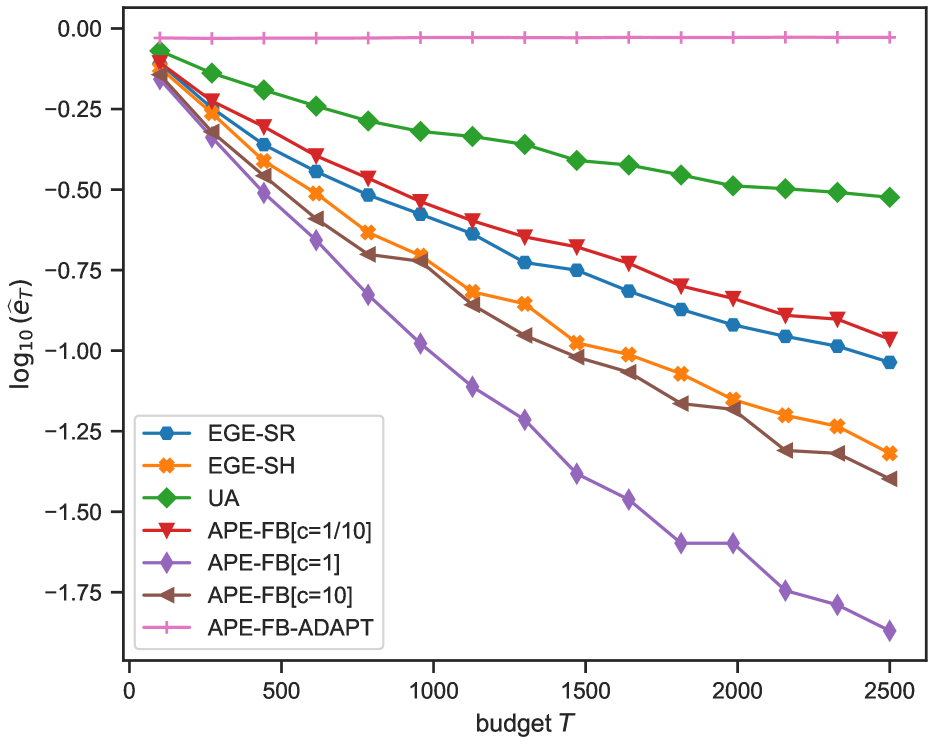
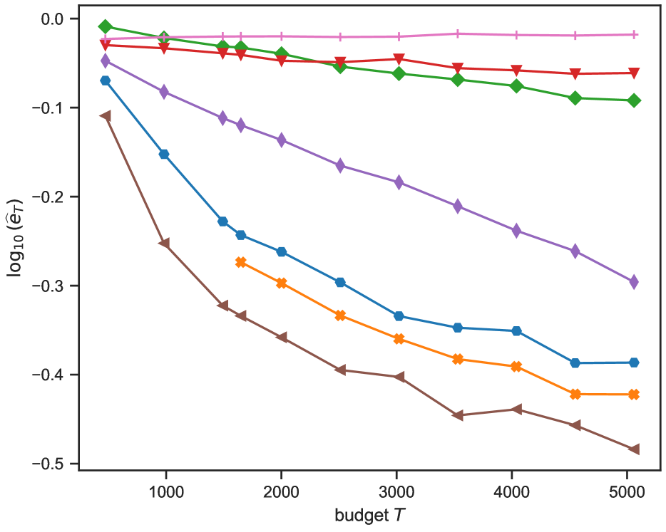
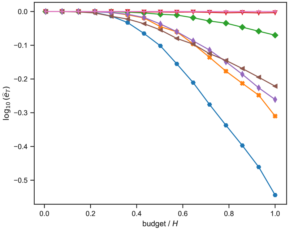
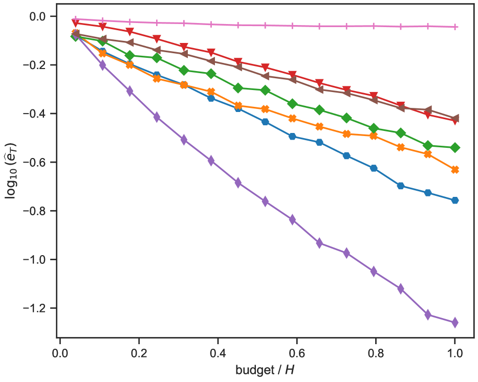
We evaluate our algorithms on synthetic and real-world tasks. We compare to Uniform Allocation (UA) and APE-FB for three parameters of the form $a_{c}=c\frac{25}{36}\frac{T-K}{H(\nu)}$, $c\in\{1/10,1,10\}$. Our guarantees on APE-FB are only valid for $c\leq 1$ and are optimal for $c=1$. We consider a heuristic version of APE-FB which adaptively estimates the hardness $H(\nu)$. We refer to this algorithm as APE-FB-ADAPT. We run the experiments 4000 times with different seeds and we report the $\log_{10}$ of the average mis-identification rate.

Figure 1: Application 1: COV-BOOST trial

Figure 2: Application 2: Sorting Networks dataset.

Figure 3: Arms on a convex Pareto set.

Figure 4: Each sub-optimal $i$ is only dominated by $i^{\star}$.

Figure 5: $K=200$ arms on the unit circle.

Figure 6: High dimension ($D=10$) with 2 group of arms.

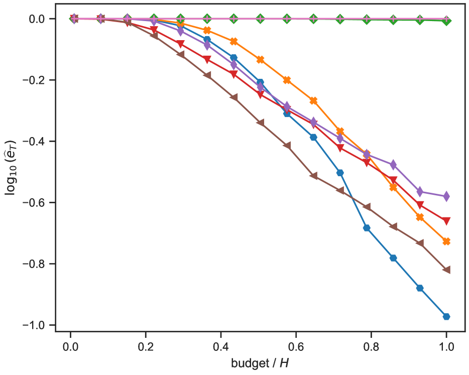
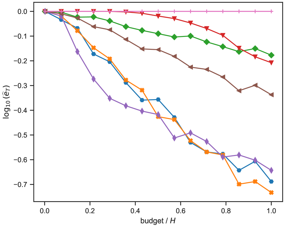
6.1 Real-world Datasets

COV-BOOST

​​(Munro et al.,, 2021) is a phase II vaccine clinical trial conducted on 2883 participants to measure the immunogenicity of different Covid-19 vaccines as a booster (third dose). Combining the first two doses received and the third dose investigated in the trial, there were $K=20$ arms and the authors reported the sample mean response and confidence intervals (based on log-normal assumption of the data) of each arm to a bunch of immunogenicity indicators. Kone et al., (2023) further extracted and processed the responses to 3 indicators (cellular response, anti-spike IgG and NT₅₀) to generate a multivariate normal bandit with $K=20,D=3$ and a diagonal covariance matrix. We use their dataset in our simulations with a total budget of $T=2500$.

Hardware Design

We use the SNW (Sorting Network Width) dataset (Zuluaga et al.,, 2012) to generate a bandit model. The dataset is made of 206 different sorting networks (devices used to sort items). The authors reported area and throughput of each network when synthetized on a FPGA (Field-Programmable Gate Array). The area is the number of FPGA slices (resources units) used during execution and the throughput is the number of samples treated per second. The goal is then to optimize both objectives simultaneously (reduced area and large throughput). The simulation process is costly and the measures may slightly vary for the same network due to randomness in the circuits. We simulate a Gaussian bandit with $K=206,D=2$ with the SNW dataset. We use a total budget of $T=5000$.

6.2 Synthetic Benchmark

We run the algorithms on different synthetic instances. For each of them, we compute the complexity $H(\nu)$ and following Audibert and Bubeck, (2010); Karnin et al., (2013) we set the total budget to $T=H(\nu)$.

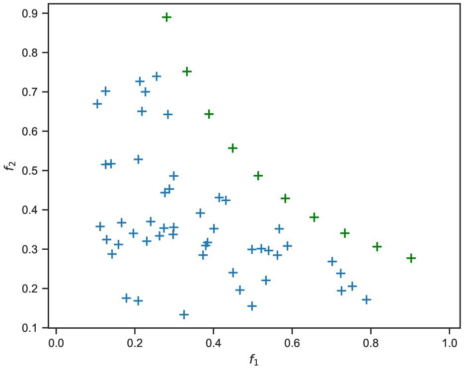
Experiment 1: Arms on a convex Pareto set. $K=60,D=2$. We choose $x_{1},\dots,x_{20}$ equally spaced in $[0.55,0.95]$ and $i=1,\dots,10$, $\bm{\theta}_{i}:=(x_{i}^{2},1/(4x_{i}^{2}))^{\intercal}$. $\bm{\theta}_{11},\dots,\bm{\theta}_{60}$ are chosen from $\left\{(x,y)\in[0.1,0.8]^{2}:xy\leq\frac{1}{5}\right\}$.

Experiment 2: Group of sub-optimal arms where each sub-optimal arm $i$ has a unique $i^{\star}$. $K=10,D=2,\lvert\mathcal{S}^{\star}\lvert=2$. For each sub-optimal arm $i$, there is a unique $j$ such that $\bm{\theta}_{i}\prec\bm{\theta}_{j}$. We choose $\bm{\theta}_{1}:=(0.4,0.75)^{\intercal},\bm{\theta}_{2}:=(0.75,0.4)^{\intercal}$ and for $i=1,\dots,4$, $\bm{\theta}_{2i+1}:=(0.45+0.2^{i},0.35-0.2^{i})^{\intercal}$, $\bm{\theta}_{2i+2}:=(0.10+0.20^{i},0.70-0.20^{i})^{\intercal}$.

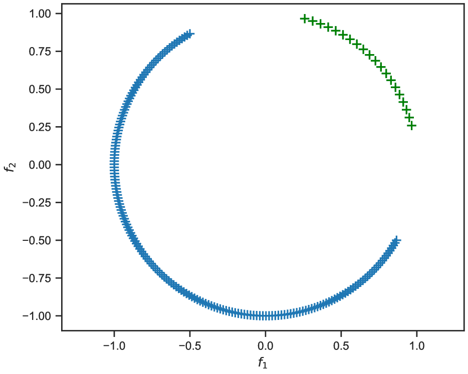
Experiment 3: Many arms on the unit circle. $K=200,D=2$ and generate n isotropic multivariate normal instance with $\sigma=1/4$. We choose $\beta_{1},\dots,\beta_{20}$ equally in $[\pi/12,\pi/2-\pi/12]$ and $\beta_{21},\dots,\beta_{200}$ equally spread in $[\pi/2+\pi/6,2\pi-\pi/6]$. For each arm $i,\bm{\theta}_{i}:=(\cos(\beta_{i}),\sin(\beta_{i}))^{\intercal}$.

Experiment 4: $D=10$ We set $K=50$ and generate $(\bm{\theta}_{1},\dots,\bm{\theta}_{30})\sim\mathcal{U}\left([0.2,0.45]^{10}\right)^{\otimes 30}$ and $(\bm{\theta}_{31},\dots,\bm{\theta}_{50})\sim\mathcal{U}\left([0.55,0.75]^{10}\right)^{\otimes 20}$

6.3 Results

In all experiments, the uniform allocation (UA) baseline is largely outperformed by both EGE-SR and EGE-SH (with no clear ordering between the two algorithms). This is particularly the case when there are many arms and for complex Pareto sets. By estimating the hardness to classify each arm, EGE eventually allocates more samples to arms that are difficult to classify, leading to a smaller error probability. APE-FB is a good competitor to our EGE algorithms however it is not robust to the hyper-parameter $a$, which requires the knowledge of $H(\nu)$ to be properly tuned. Our proposed heuristic that estimates the complexity online fails dramatically.

In Appendix G.1 we discuss the computational complexity of EGE and we detail the implementation setup. In Appendix G.2 we report additional experimental results on synthetic datasets. We illustrate the PSI-$k$ relaxation on the SNW dataset, showing that EGE-SR-$k$ can efficiently identify a subset of the Pareto set.

7 CONCLUSION

We proposed the first algorithms for Pareto set identification in the fixed-budget setting.

Our generic algorithm EGE can be coupled with different allocation and arm elimination schemes. We proved that for two instantiations, EGE-SR and EGE-SH, the probability of error decays exponentially fast with the budget, with an exponent that is un-improvable for some bandit instances. We conducted experiments showing that these algorithms consistently outperform a uniform sampling baseline and are competitive with an oracle algorithm that knows the complexity of the underlying instance.

Extensions of this work could consider variance-aware estimates of the gaps or a Bayesian setting where prior information on the means could be used to improve performance (Atsidakou et al.,, 2023). Finally, just like Successive Rejects or Sequential Halving, EGE algorithms heavily relies on the knowledge of $T$ for their tuning. In future work, we are interested in proposing anytime algorithms, that can have a small error probability for any budget $T$. We may take inspiration from some anytime algorithms recently proposed for simpler pure exploration tasks (Katz-Samuels and Scott,, 2018; Jourdan et al.,, 2023).

Acknowledgements

Cyrille Kone is funded by an Inria/Inserm PhD grant. Emilie Kaufmann acknowledges the support of the French National Research Agency under the projects BOLD (ANR-19-CE23-0026-04) and FATE (ANR22-CE23-0016-01).

Appendix A ANALYSIS OF EMPIRICAL GAP ELIMINATION

A.1 Proof of Theorem 1

We state below an important lemma used in the proof of Theorem 1. For each sub-optimal arm $i$, we define $i^{\star}$ to be an arbitrary element in $\operatorname*{argmax}_{k\in\mathcal{S}^{\star}}\operatorname{m}(i,k)$, which by definition yields $\Delta_{i}^{\star}=\operatorname{m}(i,i^{\star})$. Introducing the property

$$\mathcal{P}_{r}:=\left\{\forall i\notin\mathcal{S}^{\star},i\in A_{r}\Rightarrow i^{\star}\in A_{r}\right\},$$

the first step of the proof consists in proving that $\mathcal{P}_{r}$ holds for all $r$. To do so, we introduce several intermediate results whose proofs are gathered in Appendix B.

The first one controls the deviation of the empirical $\operatorname{{{M}}}(i,j;r)$ and $\operatorname{{{m}}}(i,j;r)$ from their actual values.

Lemma 5.

On the event $\mathcal{E}_{c}^{1}$, for all $r\in[R]$ and $i,j\in A_{r}$, if $i\in\mathcal{S}^{\star}$ or $j\in\mathcal{S}^{\star}$

$$\lvert\operatorname{{{M}}}(i,j;r)-\operatorname{M}(i,j)\lvert\leq c\Delta_{(\lambda_{r+1}+1)}\;\text{and}$$

$$\lvert\operatorname{{{m}}}(i,j;r)-\operatorname{m}(i,j)\lvert\leq c\Delta_{(\lambda_{r+1}+1)}.$$

The second one builds on it to prove that the empirical gaps cannot be too far from their true gaps, if $\mathcal{P}_{r}$ holds. It is complementary to Lemma 2 stated in the main paper.

Lemma 6.

Assume that $\mathcal{E}_{1}^{c}$ holds and let $r\in[R]$ such that $\mathcal{P}_{r}$ holds. Then for any $i\in A_{r}$

$$\widehat{\Delta}_{i,r}-\Delta_{i}\geq\begin{cases}-2c\Delta_{(\lambda_{r+1}+1)}&\text{ if }i\in\mathcal{S}^{\star},\\ -c\Delta_{(\lambda_{r+1}+1)}&\text{ else.}\end{cases}$$

Lemma 7.

Let $c>0$ and assume $\mathcal{E}_{c}^{1}$ holds. At round $r\in[R]$, for any sub-optimal arm $i\in A_{r}$, if $i^{\star}\in A_{r}$ and $i^{\star}$ does not empirically dominate $i$ then $\Delta_{i}^{\star}\leq c\Delta_{(\lambda_{r+1}+1)}$.

We are now ready to prove the following key result.

See 3

Proof.

We assume that the event $\mathcal{E}_{c}^{1}$ holds and we prove the result by induction on $r$.

$\mathcal{P}_{r}$ trivially holds for $r=1$ as all arms are active. Let $r\geq 1$ such that hat $\mathcal{P}_{r}$ holds. We shall prove that for any $i\in A_{r+1}\cap(\mathcal{S}^{\star})^{\mathsf{c}}$, $i^{\star}$ cannot be deactivated at the end of round $r$. A first observation is that the empirical gap $\widehat{\Delta}_{i,r}$ of each arm $i$ satisfies

$$\widehat{\Delta}_{i,r}=\max\left(\widehat{\Delta}_{i,r}^{\star},\widehat{\delta}_{i,r}^{\star}\right)$$ (8)

which follows from the fact that when $i\in S_{r}$, $\widehat{\Delta}_{i,r}^{\star}<0\leq\widehat{\delta}_{i,r}^{\star}$ and when $i\in A_{r}\backslash S_{r}$, $\widehat{\delta}_{i,r}^{\star}<0\leq\widehat{\Delta}_{i,r}^{\star}$. Using Lemma 6 and the inductive hypothesis permits to prove that

$$\forall i\in A_{r},\ \ \widehat{\Delta}_{i,r}\geq\Delta_{i}-2c\Delta_{(\lambda_{r+1}+1)}.$$ (9)

To prove that $\mathcal{P}_{r+1}$ holds, we proceed by contradiction and assume that there exists a sub-optimal arm $i\in A_{r}$ (and therefore $i^{\star}\in A_{r}$ by $\mathcal{P}_{r}$) such that $i\in A_{r+1}$ and $i^{\star}\in A_{r}\backslash A_{r+1}$.

A first observation is that as there are $\lambda_{r+1}$ arms in $A_{r+1}$ and $i^{\star}$ is deactivated at the end of round $r$, there exists an arm $a_{r}\in A_{r+1}\cup\{i^{\star}\}$ such that $\Delta_{a_{r}}\geq\Delta_{(\lambda_{r+1}+1)}$ and $\widehat{\Delta}_{i^{\star}}\geq\widehat{\Delta}_{a_{r}}$. We now consider two cases depending on whether $i^{\star}$ is empirically optimal or empirically sub-optimal.

Case 1: arm $i^{\star}\notin S_{r}$ i.e. $i^{\star}$ is empirically sub-optimal.

We have

$$\max_{j\in A_{r}\backslash\{i^{\star}\}}\operatorname{{{m}}}(i^{\star},j;r):=\widehat{\Delta}_{i^{\star},r}^{\star}=\widehat{\Delta}_{i^{\star},r}\geq\widehat{\Delta}_{a_{r},r}$$

Using Lemma 5 (on the LHS) and Equation (9) (on the RHS) yields

$$\max_{j\in A_{r}\backslash\{i^{\star}\}}\operatorname{m}(i^{\star},j) \geq \Delta_{a_{r}}-3c\Delta_{(\lambda_{r+1}+1)},$$

$$\geq (1-3c)\Delta_{(\lambda_{r+1}+1)}\;,$$

where the last inequality follows since $\Delta_{a_{r}}\geq\Delta_{(\lambda_{r+1}+1)}$. As $i^{\star}$ is optimal, the LHS of the previous inequality is negative. So it follows that $0\geq(1-3c)\Delta_{(\lambda_{r+1}+1)}$ which yields a contradiction if $3c<1$.

Case 2: arm $i^{\star}\in S_{r}$ i.e. $i^{\star}$ is empirically optimal.

We first prove that $i^{\star}$ does not empirically dominate $i$. Indeed, if $i$ were dominated by $i^{\star}$, we would have $i\notin S_{r}$, so $\widehat{\Delta}_{i,r}=\widehat{\Delta}_{i,r}^{\star}>0$ and since $i^{\star}\in S_{r}$,

$$\widehat{\Delta}_{i^{\star},r}=\widehat{\delta}^{\star}_{i^{\star},r} \leq (\operatorname{{{M}}}(i,i^{\star};r))^{+}+(\widehat{\Delta}_{i,r}^{\star})^{+},$$ (10)

$$= 0+\Delta_{i,r}.$$ (11)

Recalling that $i\in A_{r+1}$ we also have $\widehat{\Delta}_{i^{\star},r}\geq\widehat{\Delta}_{i,r}$, which combined with Equation (11) yields

$$\widehat{\Delta}_{i^{\star},r}=\widehat{\Delta}_{i,r}.$$ (12)

However, the tie-breaking rule of EGE ensures that Equation (12) is not possible since $i^{\star}\in S_{r}$ and it is deactivated while $i\in A_{r+1}\cap(S_{r})^{\mathsf{c}}$ (in case of an equality in the gaps, empirically sub-optimal arms are removed). Therefore $i$ is not empirically dominated by $i^{\star}$. Hence, by 7

$$\Delta_{i}^{\star}\leq c\Delta_{(\lambda_{r+1}+1)}.$$ (13)

Moreover, since $a_{r}\in A_{r+1}\cup\{i^{\star}\}$, using the definition of $\widehat{\Delta}_{i^{\star},r}$ yields

$$\operatorname{{{M}}}(i,i^{\star};r)^{+}+(\widehat{\Delta}_{i,r}^{\star})^{+}\geq\widehat{\Delta}_{a_{r},r}$$

Using Lemma 5, Lemma 6 applied to $i$ and Equation (9) applied to $a_{r}$, we obtain

$$\operatorname{M}(i,i^{\star})^{+}+\Delta_{i}^{\star} \geq \Delta_{a_{r}}-5c\Delta_{(\lambda_{r+1}+1)}$$

$$\geq (1-5c)\Delta_{(\lambda_{r+1}+1)}$$

so

$$\Delta_{i}^{\star}\geq(1-5c)\Delta_{(\lambda_{r+1}+1)}.$$ (14)

Combining this inequality with Equation (13) yields a contradiction if $6c<1$. ∎ Before proving Theorem 1 we need Lemma 8 to upper-bound $\mathbb{P}(\overline{(\mathcal{E}_{c}^{1})})$ for any $c>0$.

Lemma 8.

For any $c>0$,

$$\mathbb{P}(\overline{(\mathcal{E}_{c}^{1})})\leq 2\lvert\mathcal{S}^{\star}\lvert(K-1)DR\exp\left(-\frac{c^{2}\widetilde{T}^{R,\bm{t},\bm{\lambda}}(\nu)}{4\sigma^{2}}\right).$$

We can now prove Theorem 1. See 1

Proof.

We show that on $\mathcal{E}_{c}^{1}$, every arm is well classified so the recommended set is the true Pareto optimal set. First by Lemma 3 we know that on $\mathcal{E}_{c}^{1}$, the property $\left(i\in A_{r}\cap(\mathcal{S}^{\star})^{\mathsf{c}}\Rightarrow i^{\star}\in A_{r}\right)$ holds for every $r\in[R]$. As in the proof of Lemma 3 (see Equation (9)), this permits to prove in Lemma 6

$$\forall r\in[R],\forall i\in A_{r},\ \ \widehat{\Delta}_{i,r}\geq\Delta_{i}-2c\Delta_{(\lambda_{r+1}+1)}$$ (15)

We now establish that at the end of every round $r\in[R]$ no mis-classification can occur. That is for every arm $i\in A_{r}\backslash A_{r+1}$:

1. if $i\notin S_{r}$ (that is, $i$ is added to $D_{r}$) then $i\notin\mathcal{S}\star$,

2. if $i\in S_{r}$ (that is, $i$ is added to $B_{r}$) then $i\in\mathcal{S}^{\star}$ .

Let $i\in A_{r}\backslash A_{r+1}$. Since $\lambda_{r+1}=\lvert A_{r+1}\lvert$ should remain active at the end of round $r$, if $i$ is removed at the end of the round, there exists $a_{r}\in A_{r+1}\cup\{i\}$ such that $\Delta_{a_{r}}\geq\Delta_{(\lambda_{r+1}+1)}$ and $a_{r}$ has a smaller empirical gap than $i$.

Case 1: $i\notin S_{r}$ i.e. $i$ is empirically sub-optimal.

As $a_{r}\in A_{r+1}\cup\{i\}$ has a smaller empirical gap than $i$, we have

$$\widehat{\Delta}_{i,r}^{\star} \geq \widehat{\Delta}_{a_{r},r},$$

Assume by contradiction $i\in\mathcal{S}^{\star}$. Using Lemma 5 and Equation (15) yields

$$\max_{j\in A_{r}\backslash\{i\}}\operatorname{m}(i,j) \geq \Delta_{a_{r}}-3c\Delta_{(\lambda_{r+1}+1)}\geq(1-3c)\Delta_{(\lambda_{r+1}+1)},$$

When $3c<1$, the RHS of Equation A.1 is positive, so this inequality yields

$$\max_{j\in A_{r}\backslash\{i\}}\operatorname{m}(i,j)>0,$$

that is there exists $j\in A_{r}$ such that

$$\operatorname{m}(i,j)>0$$

so there exists $j$ such that $\bm{\theta}_{i}\prec\bm{\theta}_{j}$, which contradicts the assumption $i\in\mathcal{S}^{\star}$. Therefore, $i\notin\mathcal{S}^{\star}$: $i$ is a sub-optimal arm.

Case 2: $i\in S_{r}$ i.e. $i$ is empirically optimal.

Since $a_{r}$ has a larger empirical gap than $i$ and $i\in S_{r}$, we have

$$\min_{j\in A_{r}\backslash\{i\}}\operatorname{M}(i,j;r)\geq\widehat{\delta}_{i}^{\star}\geq\widehat{\Delta}_{a_{r},r}$$ (16)

Assume by contradiction that $i$ is sub-optimal. By Lemma 3 (for $c<1/6$), $i^{\star}\in A_{r}$. Combining with (16) yields

$$\operatorname{M}(i,i^{\star};r)\geq\widehat{\Delta}_{a_{r},r}.$$

Further using Lemma 5 and Equation (15) yields

$$\operatorname{M}(i,i^{\star})\geq(1-3c)\Delta_{(\lambda_{r+1}+1)}.$$

Then by taking $6c<1$, the RHS of the inequality is positive so

$$\operatorname{M}(i,i^{\star})>0,$$ (17)

which is not possible as $\bm{\theta}_{i}\prec\bm{\theta}_{i^{\star}}.$ Therefore, $i\in\mathcal{S}^{\star}$: it is an optimal arm.

This proves that on the event $\mathcal{E}_{c}^{1}$, $B_{R}\subseteq\mathcal{S}^{\star}$ and $D_{R}\subseteq(\mathcal{S}^{\star})^{\mathsf{c}}$. Moreover, if there is a remaining active arm in $A_{R+1}$ (which happens if and only if $\lambda_{R+1}=1$), this arm has to be optimal by Lemma 3. Therefore, on $\mathcal{E}_{c}^{1}$, the set recommended by EGE is $\widehat{S}_{T}=B_{R}\cup A_{R+1}=\mathcal{S}^{\star}$.

As a consequence, for any $0<x<1/6$, letting $c_{x}=1/6-x$ we have

$$e^{\text{EGE}}_{T}(\nu)\leq\mathbb{P}(\overline{(\mathcal{E}_{c_{x}}^{1})}),$$

which by Lemma 8 yields

$$e^{\text{EGE}}_{T}(\nu)\leq 2\lvert\mathcal{S}^{\star}\lvert(K-1)DR\exp\left(-\frac{c_{x}^{2}\widetilde{T}^{R,\bm{t},\bm{\lambda}}}{4\sigma^{2}}\right).$$

We conclude by letting $x\rightarrow 0$. ∎

A.2 Proof of Corollary 1.1

See 1.1

Proof.

The result follows from Theorem 1 and the expression of the arm schedule and allocation vector. For EGE-SR, we have $R=K-1$, $\lambda_{r}^{\text{SR}}=K+1-r$ and $t^{\text{SR}}_{r}=n_{r}^{\text{SR}}-n_{r-1}^{\text{SR}}$ where $n_{r}^{\text{SR}}=\left\lceil\frac{1}{\overline{\log(K)}}\frac{T-K}{K+1-r}\right\rceil$, which yields

$$\widetilde{T}^{R,\bm{t}^{\textrm{SR}},\bm{\lambda}^{\textrm{{SR}}}}(\nu) := \min_{r\in[K-1]}n_{r}^{\text{SR}}\Delta_{(\lambda_{r+1}^{\text{SR}}+1)}^{2},$$

$$\geq \min_{r\in[K-1]}\frac{\Delta_{(K+1-r)}^{2}}{\overline{\log(K)}}\frac{T-K}{K+1-r},$$

$$= \frac{T-K}{\overline{\log}(K)}\frac{1}{\max_{r\in\{2,\dots K\}}r\Delta_{(r)}^{-2}}$$

$$= \frac{T-K}{\overline{\log}(K)}\frac{1}{H_{2}(\nu)}.$$

For EGE-SH we have $R=\lceil\log_{2}(K)\rceil$, $n_{r}^{\textrm{SH}}:=\sum_{s=1}^{r}t_{s}^{\textrm{SH}}\geq\frac{T}{\lambda_{r}^{\textrm{SH}}\lceil\log_{2}(K)\rceil}$ and $\lambda_{r}^{\textrm{SH}}\leq 2(\lambda_{r+1}^{\textrm{SH}}+1)$. Then

$$\widetilde{T}^{R,\bm{t}^{\textrm{SH}},\bm{\lambda}^{\textrm{SH}}}(\nu) :=\min_{r\in\{1,\dots,\lceil\log_{2}(K)\rceil\}}n_{r}^{\textrm{SH}}\Delta_{(\lambda_{r+1}^{\textrm{SH}}+1)}^{2},$$

$$\geq\min_{r\in\{1,\dots,\lceil\log_{2}(K)\rceil\}}\frac{\Delta_{(\lambda_{r+1}^{\textrm{SH}}+1)}^{2}}{\lambda_{r+1}^{\textrm{SH}}+1}\times\frac{T}{2\lceil\log_{2}(K)\rceil},$$

$$=\frac{T/(2\lceil\log_{2}(K)\rceil)}{\max_{r\in\lvert\lceil\log_{2}(K)\rceil\lvert}(\lambda_{r+1}^{\textrm{SH}}+1)\Delta_{(\lambda_{r+1}^{\textrm{SH}}+1)}^{-2}}$$

$$\geq\frac{T}{2H_{2}(\nu)\lceil\log_{2}(K)\rceil}.$$

∎

A.3 Analysis of EGE-SR-$k$

In this section, we analyze EGE-SR-$k$ and bound its stopping time.

We define for any $c>0$ and $t\in[K-1]$:

$$\mathcal{E}_{c}^{2}(t):=\bigcap_{r\in[t]}\bigcap_{i\in\mathcal{S}^{\star}}\bigcap_{j\in[K]}\;\left\{\left\|(\bm{\widehat{\theta}}_{i,n_{r}}-\bm{\widehat{\theta}}_{j,n_{r}})-(\bm{\theta}_{i}-\bm{\theta}_{j})\right\|_{\infty}\leq c\Delta_{(K+1-r)}^{(k)}\right\}$$

and in particular

$$\mathcal{E}_{c}^{2}:=\mathcal{E}_{c}^{2}(K-1).$$

We define $\tilde{k}=\min(k,\lvert\mathcal{S}^{\star}\lvert)$.

For any round $r$, let $\alpha(r)=\lvert B_{r}\lvert$ denote the number of arms so far identified as optimal at the beginning of round $r$. We denote these arms by $a_{1},\dots,a_{\alpha(r)}$. We say that the algorithm has made an error before round $r$ if $B_{r}\cap(\mathcal{S}^{\star})^{\mathsf{c}}\neq\emptyset$ or $D_{r}\cap\mathcal{S}^{\star}\neq\emptyset$. We will show that on $\mathcal{E}_{c}^{2}(t)$, the algorithm does not make any error until the end of round $\tau_{k}^{t}$ such that $\alpha(\tau_{k}^{t}+1)=\tilde{k}$.

Lemma 9.

Let $c<1/6,t\in[R]$ and $k\leq\lvert\mathcal{S}^{\star}\lvert$. Let $\tau_{k}^{t}:=\min\{r\in[t]:\alpha(r+1)=\tilde{k}\}\land t$. On the event $\mathcal{E}_{c}^{2}(t)$, the algorithm makes no error until the end round $\tau_{k}^{t}$ and for any $r\leq\tau_{k}^{t}+1$, if $j\in A_{r}$ is a sub-optimal arm then $j^{\star}\in A_{r}$. In particular, on the event $\mathcal{E}_{c}^{2}(t)$, $\{a_{1},\dots,a_{\alpha(\tau_{k}^{t}+1)}\}\subset\mathcal{S}^{\star}$.

Said otherwise, this lemma states that the first arms that will be declared as optimal by EGE-SR-$k$ will be actually optimal if $\mathcal{E}_{c}^{2}(t)$ holds for $c$ small enough.

Proof.

In the sequel we assume that $\mathcal{E}_{c}^{2}(t)$ holds. We prove the correctness by induction on the round $r$. Let $r\in[t]$ and let $B_{r}=\left\{a_{1},\dots,a_{\alpha(r)}\right\}$ denote the arms so far identified as optimal. Let $\mathcal{H}_{r}$ be the property “for any sub-optimal arm $i\in A_{r}$, $i^{\star}\in A_{r}$ and no error occurred so far”.

$\mathcal{H}_{r}$ trivially holds for $r=1$ and $\alpha(1)=0$. We now assume that it holds until the beginning of round $r$ and that $\alpha(r)<\tilde{k}$. We will show that the arm $i_{r}$ de-activated at the end of round $r$ is well classified and that for any sub-optimal arm $j\in A_{r+1}$, $j^{\star}\in A_{r+1}$.

Lemma 10.

If $\mathcal{H}_{r}$ holds at round $r$ and $\alpha(r)<\tilde{k}$, there exists $a\in A_{r}$ such that $\Delta_{a}^{(k)}=\Delta_{a}$ and $\Delta_{a}^{(k)}\geq\Delta_{(K+1-r)}^{(k)}.$

Proof.

At the beginning of round $r$, it remains $K-r+1$ active arms so there exists $a\in A_{r}$ such that $\Delta_{a}^{(k)}\geq\Delta_{(K+1-r)}^{(k)}$. If $a$ is sub-optimal then $\Delta_{a}^{(k)}=\Delta_{a}$. Otherwise, if $a$ is an optimal arm, since $\alpha(r)<\tilde{k}$ and no error has occurred so for (by assumption) then there exists one of the optimal arms $a^{\prime}\in A_{r}$ (one of those with the $\tilde{k}$ largest gaps) such that $\Delta_{a^{\prime}}^{(k)}=\Delta_{a^{\prime}}$ and $\Delta_{(K+1-r)}^{(k)}\leq\Delta_{a}^{(k)}\leq\Delta_{a^{\prime}}^{(k)}$.

∎

Lemma 5 still holds for the event $\mathcal{E}_{c}^{2}(t)$ with the modified gaps introduced earlier. We state the following lemma which is similar to 2.

Lemma 11.

Assume that the event $\mathcal{E}_{c}^{2}(t)$ holds. Let $r\in[t]$ and assume that for any sub-optimal arm $j\in A_{r}$, $j^{\star}\in A_{r}$. Then, for any sub-optimal arm $i\in A_{r}$,

$$\lvert\widehat{\Delta}_{i,r}^{\star}-\Delta_{i}^{\star}\lvert\leq 2c\Delta_{({K+1-r})}^{(k)}$$

and for any optimal arm $i\in A_{r}$,

$$\widehat{\delta}_{i,r}^{\star}\geq\Delta_{i}-2c\Delta_{({K+1-r})}^{(k)}.$$

As already noted in the proof of Lemma 3 and Lemma 6, it is simple to see that the empirical gap $\widehat{\Delta}_{i,r}$ of each arm $i$ satisfies

$$\widehat{\Delta}_{i,r}=\max\left(\widehat{\Delta}_{i,r}^{\star},\widehat{\delta}_{i,r}^{\star}\right).$$ (18)

It follows from the fact that when $i\in S_{r}$, $\widehat{\Delta}_{i,r}^{\star}<0\leq\widehat{\delta}_{i,r}^{\star}$ and when $i\in A_{r}\backslash S_{r}$, $\widehat{\delta}_{i,r}^{\star}<0\leq\widehat{\Delta}_{i,r}^{\star}$.

Using Lemma 11 and the inductive hypothesis $\mathcal{H}_{r}$ permits to prove that

$$\forall i\in A_{r},\ \ \widehat{\Delta}_{i,r}\geq\Delta_{i}-2c\Delta_{({K+1-k})}^{(k)}$$ (19)

We split the proof in three steps to prove that $\mathcal{H}_{r+1}$ holds.

Step 1:

$i_{r}$ is well classified. Let $i_{r}$ be empirically sub-optimal ($i_{r}\notin S_{r}$) and assume $i_{r}\in\mathcal{S}^{\star}$.

Since $i_{r}$ is removed at the end of round $r$, by the inductive assumption and using Equation 19 and Lemma 5 (adapted) we have

$$\max_{j\in A_{r}\backslash\{i_{r}\}}\operatorname{{{m}}}(i_{r},j)\geq\Delta_{i}-3c\Delta_{(K+1-r)}^{(k)},\;\forall i\in A_{r}.$$ (20)

By Lemma 10, there exists $a\in A_{r}$ such that $\Delta_{a}=\Delta_{a}^{(k)}\geq\Delta_{(K+1-r)}^{(k)}$. Applying (20) to this arm $a$ yields

$$\max_{j\in A_{r}\backslash\{i_{r}\}}\operatorname{{{m}}}(i_{r},j)\geq(1-3c)\Delta_{(K+1-r)}^{(k)}.$$ (21)

Recalling that $c<1/6$ we see that the LHS of (21) is positive, so there exists $j$ such that

$$\bm{\theta}_{i_{r}}\prec\bm{\theta}_{j}$$

which contradicts the assumption $i_{r}\in\mathcal{S}^{\star}$.

Now if $i_{r}$ is empirically optimal, i.e $i_{r}\in S_{r}$ assume $i_{r}$ is a sub-optimal arm that is $i_{r}\notin\mathcal{S}^{\star}$. By the hypothesis $\mathcal{H}_{r}$, $i_{r}^{\star}\in A_{r}$ and by definition of $\widehat{\Delta}_{i_{r},r}$ and since $i_{r}$ is removed, we have (Lemma 5 and Equation 19)

$$\operatorname{M}(i_{r},i_{r}^{\star})\geq\Delta_{i}-3c\Delta_{(K+1-r)}^{(k)}\quad\forall i\in A_{r}.$$ (22)

Using Lemma 10 as before, there exists $a\in A_{r}$ such that $\Delta_{(K+1-r)}^{(k)}\leq\Delta_{a}^{(k)}=\Delta_{a}$. So the LHS of (22) is positive for $c<1/6$. That is

$$\operatorname{M}(i_{r},i_{r}^{\star})>0,$$

which is impossible as $\bm{\theta}_{i_{r}}\prec\bm{\theta}_{i_{r}^{\star}}$. This concludes the proof of this part: $i_{r}$ is well classified.

Step 2:

If $i_{r}\in\mathcal{S}^{\star}$ is an optimal arm, then no active arm is “optimally” dominated by $i_{r}$:

$$\forall i\in A_{r}\cap(\mathcal{S}^{\star})^{\mathsf{c}},i^{\star}\neq i_{r}$$

To prove this, note that we can deduce from “Step 1” that $i_{r}\in S_{r}$. By contradiction, let $i\in A_{r}\cap(\mathcal{S}^{\star})^{\mathsf{c}}$ such that $i^{\star}=i_{r}$. We claim that $i$ is not dominated by $i_{r}$. Indeed, if $i$ were dominated by $i_{r}$, we would have $i\notin S_{r}$ (i.e empirically sub-optimal) so

$$\widehat{\Delta}_{i,r}=\widehat{\Delta}_{i,r}^{\star}>0$$

and since $i_{r}\in S_{r}$, by defintion of $\widehat{\delta}_{i_{r},r}^{\star}$ and noting that $\widehat{\Delta}_{i_{r},r}\geq\widehat{\Delta}_{i,r}$, we would have

$$\widehat{\Delta}_{i_{r},r} \leq (\operatorname{{{M}}}(i,i_{r};r))^{+}+(\widehat{\Delta}_{i}^{\star})$$

$$= 0+\widehat{\Delta}_{i,r},$$

that is $\widehat{\Delta}_{i_{r},r}\leq\widehat{\Delta}_{i,r}$. However, our tie-breaking ensures that this inequality is impossible: since $i_{r}\in S_{r},i\notin S_{r}$ and $i_{r}$ is deactivated we have $\widehat{\Delta}_{i_{r},r}>\widehat{\Delta}_{i,r}$. Therefore $i$ is not empirically dominated by $i_{r}$. Moreover, since $i_{r}=i^{\star}$ (by assumption), Lemma 7 (it trivially holds with the modified gaps) yields

$$\Delta^{\star}_{i}\leq c\Delta_{(K+1-r)}^{(k)}.$$ (23)

Recalling that $i_{r}$ is deactivated, we have for any arm $j\in A_{r}$,

$$(\operatorname{{{M}}}(i,i_{r};r))^{+}+(\widehat{\Delta}_{i,r}^{\star})^{+}\geq\widehat{\Delta}_{j,r}$$ (24)

On the other side, there exists $a\in A_{r}$ such that $\Delta_{(K+1-r)}^{(k)}\leq\Delta_{a}^{(k)}=\Delta_{a}$ (Lemma 10). Applying Equation (19) and Lemma 5 and taking $j=a$ in Equation 24 yields

$$(\operatorname{M}(i,i_{r}))^{+}+(\Delta_{i}^{\star})^{+}\geq(1-5c)\Delta_{(K+1-r)}^{(k)}$$

that is

$$\Delta_{i}^{\star}\geq(1-5c)\Delta_{(K+1-r)}^{(k)}.$$ (25)

Both (23) and (25) cannot hold when $c<1/6$. So for any $i\in A_{r}$

$$i^{\star}\neq i_{r}.$$

Which achieves the proof of ”Step 2”. Put together, ”Step 1&2” prove that $\mathcal{H}_{r+1}$ holds.

Step 3:

Conclusion

We have proved that if $\mathcal{H}_{r}$ holds and $\alpha(r)<\tilde{k}$ then $\mathcal{H}_{r+1}$ holds. Note that if $i_{r}\in S_{r}$ then $\alpha(r+1)=\alpha(r)+1$ otherwise $\alpha(r+1)=\alpha(r)$. Therefore, no error occurs until the end of round $\min(r^{\prime},t)$ where $r^{\prime}$ is such that $\alpha(r^{\prime}+1)=\tilde{k}$. As a consequence $B_{\tau_{k}^{t}+1}=\{a_{1},\dots,a_{\alpha(\tau_{k}^{t}+1)}\}\subset\mathcal{S}^{\star}$. And by the proof of ”Step 2”, if $j\in A_{\tau_{p}^{t}}$ is a sub-optimal arm, then $j^{\star}\in A_{\tau_{p}^{t}+1}$.

∎

See 3

Proof.

The proof is a direct consequence of Lemma 9 and Hoeffding’s inequality. Indeed, Lemma 9 yields that EGE-SR-$k$ is correct on the event $\mathcal{E}_{c}^{2}$ for $c<1/6$. Therefore, for any $0<c<1/6$

$$e_{T,k}(\nu)\leq\mathbb{P}(\overline{(\mathcal{E}_{c}^{2})}).$$

Letting $0<c<1/6$ fixed, by union bound and Hoeffing’s inequality (as in the proof of Lemma 8) it follows that

$$\mathbb{P}(\overline{(\mathcal{E}_{c}^{2})})\leq 2(K-1)^{2}\lvert\mathcal{S}^{\star}\lvert D\exp\left(-c^{2}\frac{T-K}{4\sigma^{2}H_{2}^{(k)}\overline{\log}(K)(\nu)}\right)$$

therefore,

$$e_{T,k}(\nu)\leq 2(K-1)^{2}\lvert\mathcal{S}^{\star}\lvert D\exp\left(-c^{2}\frac{T-K}{4\sigma^{2}H_{2}^{(k)}(\nu)\overline{\log}(K)}\right)$$

and taking the limit to $1/6$ (as it holds for any $0<c<1/6$) yields the expected result. ∎

The theorem below bounds the expected stopping time and the number of samples used at stopping.

Theorem 4.

Fix $k<\lvert\mathcal{S}^{\star}\lvert$ and let $q:=K-\lvert\mathcal{S}^{\star}\lvert+k$. Then

$$\mathbb{E}[\tau] \leq q+2(K-1)\lvert\mathcal{S}^{\star}\lvert(K-q-1)qD\exp\left(-\frac{T-K}{144\sigma^{2}H_{2}^{(k)}(\nu)\overline{\log}(K)}\right)\text{ and }$$

$$\mathbb{E}[N_{\tau}] \leq N_{q}+2(K-1)\lvert\mathcal{S}^{\star}\lvert(K-q-1)qDT\exp\left(-\frac{T-K}{144\sigma^{2}H_{2}^{(k)}(\nu)\overline{\log}(K)}\right).$$

This result suggests that for this relaxed problem, the algorithm might not need to use the whole budget, in particular when $T$ is large. For example, consider a setting $[K]=\mathcal{S}^{\star}$ then $q=k$ and we roughly use $N_{k}$ samples which can be way smaller than $N_{K-1}$.

Proof.

The idea is to show that if the algorithm has not stopped after round $q$ then some high probability event must not hold. Let $c<1/6$ be fixed. We have

$$\mathbb{E}[\tau] \leq q+\mathbb{E}[\tau\mathbb{I}\{\tau>q\}],$$

$$\leq q+\sum_{s=q+1}^{K-1}\mathbb{P}(\tau\geq s).$$

We claim that for any $s>q$,

$$\{\tau\geq s\}\subset\overline{(\mathcal{E}_{c}^{2}(q))}.$$

Indeed,

$$\tau\geq s \Longrightarrow \tau>q$$

$$\Longrightarrow \alpha(q+1)<k,$$

However, by Lemma 9, if $\mathcal{E}_{c}^{2}(q)$ holds and $\alpha(q+1)<k$ then no error has occured until the end of round $q$, therefore $D_{q}=(\mathcal{S}^{\star})^{\mathsf{c}}$ and $\lvert B_{q}\lvert=k$, which is not possible as $\alpha(q+1)<k$. So $\tau\geq s\Longrightarrow(\mathcal{E}_{c}^{2}(q)$ does not hold). Then

$$\mathbb{E}[\tau] \leq q+\sum_{s=q+1}^{K-1}\mathbb{P}(\overline{(\mathcal{E}_{c}(q))}),$$ (26)

$$\leq q+\sum_{s=q+1}^{K-1}2(K-1)\lvert\mathcal{S}^{\star}\lvert qD\exp\left(-c^{2}\frac{T-K}{4\sigma^{2}H_{2}^{(k)}(\nu)\overline{\log}(K)}\right),$$ (27)

$$\leq q+2(K-1)\lvert\mathcal{S}^{\star}\lvert(K-q-1)qD\exp\left(-c^{2}\frac{T-K}{4\sigma^{2}H_{2}^{(k)}(\nu)\overline{\log}(K)}\right).$$ (28)

Similarly, we have

$$\mathbb{E}[N_{\tau}]\leq N_{q}+(N_{\tau}\mathbb{I}_{\tau>q}).$$

Then,

$$\mathbb{E}[N_{\tau}] \leq N_{q}+\sum_{s=q+1}^{K-1}N_{s}\mathbb{P}(\tau\geq s)$$

$$\leq N_{q}+\sum_{s=q+1}^{K-1}N_{s}\mathbb{P}(\overline{(\mathcal{E}_{c}^{2}(q))})$$

$$\leq N_{q}+2(K-1)\lvert\mathcal{S}^{\star}\lvert qD\exp\left(-c^{2}\frac{T-K}{4\sigma^{2}H_{2}^{(k)}(\nu)\overline{\log}(K)}\right)\sum_{s=q+1}^{K-1}N_{s}.$$

Simple algebra yields for any $r\in[K-1],$

$$N_{r} = (K-r)n_{r}+\sum_{s=1}^{r}n_{s},$$

$$\leq \frac{T-K}{\overline{\log}(K)}+(K-r)+r+\frac{T-K}{\overline{\log}(K)}\sum_{s=1}^{r}\frac{1}{K+1-s}$$

$$= \frac{T-K}{\overline{\log}(K)}\left(1+\sum_{s=K+1-r}^{K}s^{-1}\right)+K$$

$$\leq T.$$

Therefore,

$$\mathbb{E}[N_{\tau}] \leq N_{q}+2(K-1)\lvert\mathcal{S}^{\star}\lvert(K-q-1)qDT\exp\left(-c^{2}\frac{T-K}{4\sigma^{2}H_{2}^{(k)}(\nu)\overline{\log}(K)}\right).$$ (29)

As (28) and (29) holds for any $c<1/6$ taking the limit for a sequence $c_{x}\rightarrow 1/6$ yields the expected constants in the exponent, which achieves the proof. ∎

Appendix B CONCENTRATION RESULTS

In this section we prove the concentration results used in Appendix A. We recall the definition of the good event:

$$\mathcal{E}_{c}^{1}\! := \!\bigcap_{r\in[R]}\bigcap_{i\in\mathcal{S}^{\star}}\bigcap_{j\in[K]}\left\{\left\|(\bm{\widehat{\theta}}_{i,n_{r}}\!-\bm{\widehat{\theta}}_{j,n_{r}})-(\bm{\theta}_{i}\!-\bm{\theta}_{j})\right\|_{\infty}\!\!\leq c\Delta_{(\lambda_{r+1}+1)}\right\}\;.$$

B.1 Proof of Lemma 5

See 5

Proof.

Assume $i\in\mathcal{S}^{\star}$ or $j\in\mathcal{S}^{\star}$. We have

$$\lvert\operatorname{{{M}}}(i,j;r)-\operatorname{M}(i,j)\lvert = \left\lvert\max_{d}\left[{\widehat{\theta}}_{i,n_{r}}^{d}-{\widehat{\theta}}_{j,n_{r}}^{d}\right]-\max_{d}\left[\theta_{i}^{d}-\theta_{j}^{d}\right]\right\lvert,$$

$$\overset{(a)}{\leq} \max_{d}\left\lvert({\widehat{\theta}}_{i,n_{r}}^{d}-{\widehat{\theta}}_{j,n_{r}}^{d})-(\theta_{i}^{d}-\theta_{j}^{d})\right\lvert,$$

$$= \left\|(\bm{\widehat{\theta}}_{i,n_{r}}-\bm{\widehat{\theta}}_{j,n_{r}})-(\bm{\theta}_{i}-\bm{\theta}_{j})\right\|_{\infty},$$

$$\overset{(b)}{\leq} c\Delta_{(\lambda_{r+1}+1)}.$$

where $(a)$ follows by reverse triangle inequality and $(b)$ holds on the event $\mathcal{E}_{c}^{1}$. The second part of the lemma follows from

$$\lvert\operatorname{{{m}}}(i,j;r)-\operatorname{m}(i,j)\lvert = \lvert-\operatorname{{{M}}}(i,j;r)+\operatorname{M}(i,j)\lvert,$$

as $\operatorname{M}(i,j)=-\operatorname{m}(i,j)$ and $\operatorname{{{M}}}(i,j;r)=-\operatorname{{{m}}}(i,j;r)$. ∎

B.2 Proof of Lemma 6

We recall the definition of the property

$$\mathcal{P}_{r}=\left\{\forall i\notin\mathcal{S}^{\star},i\in A_{r}\Rightarrow i^{\star}\in A_{r}\right\}.$$

and start by proving a first intermediate result.

Lemma 12.

Assume that $\mathcal{E}_{1}^{c}$ holds and let $r\in[R]$ such that $\mathcal{P}_{r}$ holds. Then for any $i\in A_{r}$,

$$(\widehat{\Delta}_{i,r}^{\star})^{+}-(\Delta_{i}^{\star})^{+}\leq 2c\Delta_{(\lambda_{r+1}+1)}\quad\text{ and }\quad(\widehat{\Delta}_{i,r}^{\star})^{+}-(\Delta_{i}^{\star})^{+}\geq-c\Delta_{(\lambda_{r+1}+1)}.$$

Proof.

We define the $\max$ of an empty set to be $-\infty$. We first analyze the case $i\in\mathcal{S}^{\star}$. When $i\in\mathcal{S}^{\star}$, we have

$$(\Delta_{i}^{\star})^{+}=0=\left(\max_{j\in A_{r}\backslash\{i\}}\operatorname{m}(i,j)\right)^{+},$$

which yields

$$\lvert(\widehat{\Delta}_{i,r}^{\star})^{+}-(\Delta_{i}^{\star})^{+}\lvert = \left\lvert\left(\max_{j\in A_{r}\backslash\{i\}}\operatorname{{{m}}}(i,j;r)\right)^{+}-\left(\max_{j\in A_{r}\backslash\{i\}}\operatorname{{{m}}}(i,j)\right)^{+}\right\lvert,$$

$$\leq \left\lvert\left(\max_{j\in A_{r}\backslash\{i\}}\operatorname{{{m}}}(i,j;r)\right)-\left(\max_{j\in A_{r}\backslash\{i\}}\operatorname{{{m}}}(i,j)\right)\right\lvert\quad\text{(since $\lvert x^{+}-y^{+}\lvert\leq\lvert x-y\lvert)$},$$

$$\leq \max_{j\in A_{r}\backslash\{i\}}\left\lvert\operatorname{{{m}}}(i,j;r)-\operatorname{{{m}}}(i,j)\right\lvert,$$

$$\leq c\Delta_{(\lambda_{r+1}+1)},$$

where the last inequality follows from Lemma 5. We now assume that $i$ is a sub-optimal arm. Since $\mathcal{P}_{r}$ holds at round $r$, $i^{\star}\in A_{r}$ and

$$\Delta_{i}^{\star}=\max_{j\in A_{r}\backslash\{i\}}\operatorname{m}(i,j).$$

Let $\hat{i}\in\operatorname*{argmax}_{j\in A_{r}\backslash\{i\}}\operatorname{{{m}}}(i,j;r)$ then

$$(\widehat{\Delta}_{i,r}^{\star})^{+}-(\Delta_{i}^{\star})^{+} = (\operatorname{{{m}}}(i,\hat{i};r))^{+}-(\operatorname{m}(i,i^{\star}))^{+},$$ (30)

$$\geq (\operatorname{{{m}}}(i,i^{\star};r))^{+}-(\operatorname{m}(i,i^{\star}))^{+}\quad\text{(since $i^{\star}\in A_{r}$)}.$$ (31)

We further note that

$$\left\lvert(\operatorname{{{m}}}(i,i^{\star};r))^{+}-(\operatorname{m}(i,i^{\star}))^{+}\right\lvert \leq \left\lvert\operatorname{{{m}}}(i,i^{\star};r)-\operatorname{m}(i,i^{\star})\right\lvert,$$

$$\leq c\Delta_{(\lambda_{r+1}+1)},$$

which follows from Lemma 5. Combining the latter inequality with (31) yields

$$(\widehat{\Delta}_{i,r}^{\star})^{+}-(\Delta_{i}^{\star})^{+}\geq-c\Delta_{(\lambda_{r+1}+1)}.$$ (32)

We also have

$$(\widehat{\Delta}_{i,r}^{\star})^{+}-(\Delta_{i}^{\star})^{+} \leq (\operatorname{{{m}}}(i,\hat{i};r))^{+}-(\operatorname{m}(i,\hat{i}))^{+},$$

$$\leq \left\lvert\operatorname{{{m}}}(i,\hat{i};r)-\operatorname{m}(i,\hat{i})\right\lvert,$$

$$= \left\lvert\operatorname{M}(i,\hat{i})-\operatorname{{{M}}}(i,\hat{i};r)\right\lvert,$$

$$\leq \left\|(\bm{\theta}_{i}-\bm{\theta}_{\hat{i}})-(\bm{\widehat{\theta}}_{i,n_{r}}-\bm{\widehat{\theta}}_{\hat{i},n_{r}})\right\|_{\infty},$$

$$= \left\|\left(\left(\bm{\theta}_{i}-\bm{\theta}_{i^{\star}}\right)-\left(\bm{\widehat{\theta}}_{i,n_{r}}-\bm{\widehat{\theta}}_{i^{\star},n_{r}}\right)\right)+\left(\left(\bm{\theta}_{i^{\star}}-\bm{\theta}_{\hat{i}}\right)-\left(\bm{\widehat{\theta}}_{i^{\star},n_{r}}-\bm{\widehat{\theta}}_{\hat{i},n_{r}}\right)\right)\right\|_{\infty},$$

$$\leq 2c\Delta_{(\lambda_{r+1}+1)},$$

where the last inequality follows from the triangle inequality and 5. This proves the lemma. ∎

We then prove Lemma 2 which can be viewed as a “symmetric” version of Lemma 6.

See 2

Proof.

Let $i\in A_{r}\cap(\mathcal{S}^{\star})^{\mathsf{c}}$. By assumption, $i^{\star}\in A_{r}$, so

$$\Delta_{i}:=\Delta^{\star}_{i}=\max_{j\in A_{r}\backslash\{i\}}\operatorname{m}(i,j),$$

then we have

$$\lvert\widehat{\Delta}_{i,r}^{\star}-\Delta_{i}\lvert = \left\lvert\left(\max_{j\in A_{r}\backslash\{i\}}\operatorname{{{m}}}(i,j;r)\right)-\left(\max_{j\in A_{r}\backslash\{i\}}\operatorname{{{m}}}(i,j)\right)\right\lvert,$$

$$\overset{(a)}{\leq} \max_{j\in A_{r}\backslash\{i\}}\lvert\operatorname{{{m}}}(i,j;r)-\operatorname{m}(i,j)\lvert,$$

$$\leq \max_{j\in A_{r}\backslash\{i\}}\lvert\operatorname{M}(i,j)-\operatorname{{{M}}}(i,j;r)\lvert$$

,

$$\leq \max_{j\in A_{r}\backslash\{i\}}\left\|(\bm{\theta}_{i}-\bm{\theta}_{j})-(\bm{\widehat{\theta}}_{i,n_{r}}-\bm{\widehat{\theta}}_{j,n_{r}})\right\|_{\infty}$$

$$= \max_{j\in A_{r}\backslash\{i\}}\left\|\left(\left(\bm{\theta}_{i}-\bm{\theta}_{i^{\star}}\right)-\left(\bm{\widehat{\theta}}_{i,n_{r}}-\bm{\widehat{\theta}}_{i^{\star},n_{r}}\right)\right)+\left(\left(\bm{\theta}_{i^{\star}}-\bm{\theta}_{j}\right)-\left(\bm{\widehat{\theta}}_{i^{\star},n_{r}}-\bm{\widehat{\theta}}_{j,n_{r}}\right)\right)\right\|_{\infty},$$

$$\overset{(b)}{\leq} 2c\Delta_{(\lambda_{r+1}+1)},$$

where $(a)$ follows by reverse triangle inequality and $(b)$ follows by triangle inequality and Lemma 5. So we have proved the first statement of the lemma.

Before proving the second statement of the lemma, recall that

$$\widehat{\delta}_{i,r}^{\star}=\min_{j\in A_{r}\backslash\{i\}}[\operatorname{{{M}}}(i,j;r)\;\land\;(\operatorname{{{M}}}(j,i;r)^{+}+(\widehat{\Delta}_{j,r}^{\star})^{+})].$$

Let $i\in A_{r}\cap\mathcal{S}^{\star}$. For any $j\in A_{r}$ we have

$$\lvert\operatorname{{{M}}}(j,i;r)^{+}-\operatorname{M}(j,i)^{+}\lvert \leq \lvert\operatorname{{{M}}}(j,i;r)-\operatorname{{{M}}}(j,i)\lvert,$$

$$\leq c\Delta_{(\lambda_{r+1}+1)}\quad\text{(Lemma }\ref{lem:lem-ineq}),$$

and similarly

$$\lvert\operatorname{{{M}}}(i,j;r)-\operatorname{M}(i,j)\lvert\leq c\Delta_{(\lambda_{r+1}+1)}$$

which put together yields

$$\operatorname{{{M}}}(j,i;r)^{+} \geq \operatorname{M}(j,i)^{+}-c\Delta_{(\lambda_{r+1}+1)}\quad\text{and}$$ (33)

$$\operatorname{{{M}}}(i,j;r) \geq \operatorname{M}(i,j)-c\Delta_{(\lambda_{r+1}+1)}.$$ (34)

Letting $j\in A_{r}$, we have by 12

$$(\widehat{\Delta}_{j,r}^{\star})^{+}-(\Delta_{j}^{\star})^{+}\geq-c\Delta_{(\lambda_{r+1}+1)}$$ (35)

Put together, (35) and (33) yields

$$\operatorname{{{M}}}(j,i;r)^{+}+(\widehat{\Delta}_{j,r}^{\star})^{+} \geq \operatorname{M}(j,i)^{+}+(\Delta_{j}^{\star})^{+}-2c\Delta_{(\lambda_{r+1}+1)}$$

for any $j\in A_{r}$. Which combined with (34) yields

$$[\operatorname{{{M}}}(i,j;r)\land(\operatorname{{{M}}}(j,i;r)^{+}+(\widehat{\Delta}_{j,r}^{\star})^{+})]\geq[\operatorname{M}(i,j)\land(\operatorname{M}(j,i)^{+}+(\Delta_{j}^{\star})^{+})]-2c\Delta_{(\lambda_{r+1}+1)}$$

for any $j\in A_{r}$. Therefore,

$$\widehat{\delta}_{i,r}^{\star} \geq \left(\min_{j\in A_{r}\backslash\{i\}}[\operatorname{M}(i,j)\land(\operatorname{M}(j,i)^{+}+(\Delta_{j}^{\star})^{+})]\right)-2c\Delta_{(\lambda_{r+1}+1)},$$

$$\geq \left(\min_{j\in[K]\backslash\{i\}}[\operatorname{M}(i,j)\land(\operatorname{M}(j,i)^{+}+(\Delta_{j}^{\star})^{+})]\right)-2c\Delta_{(\lambda_{r+1}+1)},$$

$$= \delta_{i}^{\star}-2c\Delta_{(\lambda_{r+1}+1)}.$$

∎

Finally, we prove Lemma 6.

See 6

Proof.

Let $i\in A_{r}\cap(\mathcal{S}^{\star})^{\mathsf{c}}$. Since $i\in(\mathcal{S}^{\star})^{\mathsf{c}}$, $\Delta_{i}=\Delta_{i}^{\star}$. If $i\notin S_{r}$ then $\widehat{\Delta}_{i,r}=\widehat{\Delta}_{i,r}^{\star}$. If $i\in S_{r}$ then $\widehat{\Delta}_{i,r}=\widehat{\delta}_{i,r}^{\star}$ and

$$\widehat{\Delta}_{i,r}^{\star}\leq 0\leq\widehat{\delta}_{i,r}^{\star}$$

which follows since $i\in S_{r}$. Therefore in both cases

$$\widehat{\Delta}_{i,r}-\Delta_{i} \geq \widehat{\Delta}_{i,r}^{\star}-\Delta_{i}^{\star}$$

$$= \max_{j}\operatorname{m}(i,j;r)-\operatorname{m}(i,i_{\star})$$

$$\geq \operatorname{m}(i,i_{\star};r)-\operatorname{m}(i,i_{\star})$$

$$\geq -c\Delta_{(\lambda_{r+1}+1)}$$

where the last inequality uses 5.

Similarly, let $i\in A_{r}\cap\mathcal{S}^{\star}$. We have $\Delta_{i}=\delta_{i}^{\star}$ (1) and $\widehat{\Delta}_{i,r}=\widehat{\delta}_{i,r}^{\star}$ if $i\in S_{r}$. If $i\in A_{r}\backslash S_{r}$ (empirically sub-optimal) then

$$\widehat{\Delta}_{i,r}=\widehat{\Delta}_{i,r}^{\star}\geq 0$$

and there exists $j\in A_{r}$ such that $\bm{\widehat{\theta}}_{i,n_{r}}\prec\bm{\widehat{\theta}}_{j,n_{r}}$ so for this arm $j$, $\operatorname{{{M}}}(i,j;r)<0$. Therefore $\widehat{\delta}_{i,r}^{\star}<0$ and

$$\widehat{\delta}_{i,r}^{\star}<0\leq\widehat{\Delta}_{i,r}=\widehat{\Delta}_{i,r}^{\star}.$$

Put together we have in all cases

$$\widehat{\Delta}_{i,r}-\Delta_{i}\geq\widehat{\delta}_{i,r}^{\star}-\Delta_{i}\geq-2c\Delta_{(\lambda_{r+1}+1)},$$

where the last inequality follows from 2. ∎

B.3 Proof of Lemma 7

See 7

Proof.

We have by definition

$$\bm{\widehat{\theta}}_{i,n_{r}}\nprec\bm{\widehat{\theta}}_{i^{\star},n_{r}} \Longrightarrow \exists\;d\;:{\widehat{\theta}}_{i,n_{r}}^{d}>{\widehat{\theta}}_{i^{\star},n_{r}}^{d}$$

$$\Longrightarrow \exists\;d\;:({\widehat{\theta}}_{i,n_{r}}^{d}-\theta_{i}^{d})-({\widehat{\theta}}_{i^{\star},n_{r}}^{d}-\theta_{i^{\star}}^{d})>\theta_{i^{\star}}^{d}-\theta_{i}^{d}\geq\operatorname{m}(i,i^{\star}),$$

so

$$\left\|(\bm{\widehat{\theta}}_{i,n_{r}}-\bm{\widehat{\theta}}_{i^{\star},n_{r}})-(\bm{\theta}_{i}-\bm{\theta}_{i^{\star}})\right\|_{\infty}\geq\Delta_{i}^{\star},$$

which, on the event $\mathcal{E}_{c}^{1}$ is only possible if

$$\Delta_{i}^{\star}\leq c\Delta_{(\lambda_{r+1}+1)}.$$

∎

B.4 Proof of Lemma 8

See 8

Proof.

We have

$$\mathbb{P}(\overline{(\mathcal{E}_{c}^{1})}) \leq \sum_{r=1}^{R}\sum_{i\in\mathcal{S}^{\star}}\sum_{j\neq i}\sum_{d=1}^{D}\mathbb{P}\left(\lvert({\widehat{\theta}}_{i,n_{r}}^{d}-{\widehat{\theta}}_{j,n_{r}}^{d})-(\theta_{i}^{d}-\theta_{j}^{d})\lvert>c\Delta_{\lambda_{r+1}+1}\right),$$

$$\leq 2\lvert\mathcal{S}^{\star}\lvert(K-1)D\sum_{r}\exp\left(-\frac{c^{2}n_{r}\Delta_{\lambda_{r+1}+1}^{2}}{4\sigma^{2}}\right)\quad\text{(Hoedding's inequality)},$$

$$\leq 2\lvert\mathcal{S}^{\star}\lvert(K-1)DR\exp\left(-\frac{c^{2}\widetilde{T}^{R,\bm{t},\bm{\lambda}}(\nu)}{4\sigma^{2}}\right).$$

∎

Appendix C LOWER BOUND

In this section, we state our lower bounds for fixed-budget PSI that hold for some class of instances. The idea is to build alternative instances where the Pareto set is changed and the complexity is less than that of the base instance. To obtain a different Pareto set we can either make optimal an arm that was sub-optimal or make sub-optimal an arm that was optimal. However in doing so, we need to take care not to decrease the gap of any arm, in particular that of the arm that is shifted, otherwise the alternative instance could be harder. This is challenging as the definition of the gaps are completely different for optimal and sub-optimal arms. In the sequel we restrict to some class of instances.

We define $\mathcal{B}$ to be the set of means $\bm{\Theta}$ such that each sub-optimal arm $i$ is only dominated by a single arm, denoted by $i^{\star}$ (that has to belong to $\mathcal{S}^{\star}$) and that for each optimal arm $j$ there exists a unique sub-optimal arm which is dominated by $j$, denoted by $\underline{j}$.

We further assume that optimal arms are not too close to arms they don’t dominate: for any sub-optimal arm $i$ and optimal arm $j$ such that $\bm{\theta}_{i}\nprec\bm{\theta}_{j}$,

$$\operatorname{M}(i,j)\geq 3\max(\Delta_{i},\Delta_{\underline{j}}).$$

An instance $\nu$ belongs to $\mathcal{B}$ if its means $\bm{\Theta}=(\bm{\theta}_{1}\dots\bm{\theta}_{K})^{\intercal}$ belongs to $\mathcal{B}$. See 2

Proof.

$\nu_{1},\dots,\nu_{K}$ are distributions over $\mathbb{R}^{D}$ parameterized by their means (resp.) $\bm{\theta}_{1},\dots,\bm{\theta}_{K}$. We let $\nu:=(\nu_{1},\dots,\nu_{K})$ and $\bm{\Theta}^{(0)}:=(\bm{\theta}_{1}\dots\bm{\theta}_{K})^{\intercal}\in\mathbb{R}^{K\times D}$. We denote by $\mathcal{S}^{\star}(\nu)$ the Pareto optimal set of the bandit instance $\nu$. For all $i\in[K]$, we define $\bm{\Theta}^{(i)}:=(\bm{\theta}_{1}^{(i)}\;\dots\;\bm{\theta}_{K}^{(i)})^{\intercal}\in\mathbb{R}^{K\times D}$ (with $\bm{\theta}^{(i)}$ to be defined later) and we let $\nu^{(i)}$ denote the bandit with parameter $\bm{\Theta}^{(i)}$. Let $\mathcal{A}$ denote an algorithm for Pareto set identification in the fixed-budget setting. We further assume that for any $i\in[K]$, $\bm{\Theta}_{(i)}$ differs from $\bm{\Theta}^{(0)}$ only in line $i$:

$$\forall a\neq i,\;\bm{\theta}_{a}^{(i)}=\bm{\theta}_{a},$$ (36)

so $\nu^{(i)}$ and $\nu$ only differs in arm $i$.

We state the following lemma which is a rewriting of Lemma 16 of Kaufmann et al., (2016).

Lemma 13 (Kaufmann et al., (2016)).

Let $\nu$ and $\nu^{\prime}$ be two bandit instances such that $\mathcal{S}^{\star}(\nu)\neq\mathcal{S}^{\star}(\nu^{\prime})$. Then

$$\max\left(e_{T}^{\mathcal{A}}(\nu),e_{T}^{\mathcal{A}}(\nu^{\prime})\right)\geq\frac{1}{4}\exp\left(-\sum_{a=1}^{K}\mathbb{E}_{\nu}[T_{a}(T)]\operatorname{KL}(\nu_{i},\nu_{i}^{\prime})\right)$$

For any $i\in[K]$,

$$\bm{\theta}_{i}^{(i)}:=\begin{cases}\bm{\theta}_{i}+2\Delta_{i}e_{d_{i}}&\text{ if }i\not\in\mathcal{S}^{\star}(\nu),\\ \bm{\theta}_{i}-2\Delta_{i}e_{d_{\underline{i}}}&\text{ else.}\end{cases}$$ (37)

Let for any $i$, $\Omega(i):=\{j:\bm{\theta}_{i}\prec\bm{\theta}_{j}\}$ the set of arms that dominate $i$. We recall that for a sub-optimal arm $i$,

$$d_{i}\in\operatorname*{argmin}_{d}\left[\theta^{d}_{i^{\star}}-\theta^{d}_{i}\right].$$

We now justify that for any $i\in[K],\mathcal{S}^{\star}(\nu^{(i)})\neq\mathcal{S}^{\star}(\nu)$, by considering two cases:

• If $i\notin\mathcal{S}^{\star}(\nu)$, as $\Omega(i)=\{i^{\star}\}$ and $i$ has been increased to be larger than $i^{\star}$ on $d_{i}$, we have that $i\in\mathcal{S}^{\star}(\nu^{(i)})$.

• If $i\in\mathcal{S}^{\star}(\nu)$, since there exists $\underline{i}$ such that $\Omega(\underline{i})=\{i\}$ and $\Delta_{i}=\Delta_{\underline{i}}^{\star}$, the shifting ensures that $\bm{\theta}^{(i)}_{\underline{i}}\nprec\bm{\theta}_{i}^{(i)}$ it comes that $\underline{i}\in\mathcal{S}^{\star}(\nu^{(i)})$.

We remark that in both cases, we have either $\bm{\theta}_{i}^{(i)}=\bm{\theta}_{i}+2\Delta_{i}e_{d_{i}}$ or $\bm{\theta}_{i}^{(i)}=\bm{\theta}_{i}-2\Delta_{i}e_{d_{\underline{i}}}$. Recalling that for multivariate Gaussian distribution with the same covariance matrix, $\operatorname{KL}\left(\mathcal{N}(\bm{\theta},\Sigma),\mathcal{N}(\bm{\theta}^{\prime},\Sigma)\right)=\frac{1}{2}(\bm{\theta}-\bm{\theta}^{\prime})^{\intercal}\Sigma^{-1}(\bm{\theta}-\bm{\theta}^{\prime})$, we get for all $i$

$$\operatorname{KL}(\nu_{i},\nu_{i}^{(i)}) = 2\Delta_{i}^{2}/\sigma^{2}.$$

By applying 13, we have for any $i\in[K]$,

$$\max(e_{T}(\nu),e_{T}(\nu^{(i)})) \geq \frac{1}{4}\exp\left(-\mathbb{E}_{\nu}[T_{i}(T)]\operatorname{KL}(\nu_{i},\nu_{i}^{i})\right)$$

$$\geq \frac{1}{4}\exp\left(-\frac{2\mathbb{E}_{\nu}[T_{i}(T)]\Delta_{i}^{2}}{\sigma^{2}}\right)$$

We conclude by using the pigeonhole principle: there must exist $i\in[K]$ such that $\mathbb{E}_{\nu}[T_{i}(T)]\leq\frac{T}{{H}(\nu){\Delta}_{i}^{2}}$. Therefore, there exists $i\in[K]$ such that

$$\max(e_{T}(\nu),e_{T}(\nu^{(i)}))\geq\frac{1}{4}\exp\left(-\frac{2T}{\sigma^{2}H(\nu)}\right).$$

It remains to show that for any $i\in[K],H(\nu^{(i)})=H(\nu)$. We introduce the following notation for any arms $p,q$

$$\operatorname{M}^{i}(p,q) := \max_{d}[(\theta_{p}^{i})^{d}-(\theta_{q}^{i})^{d}],$$

$$\operatorname{m}^{i}(p,q) := -\operatorname{M}^{i}(p,q),$$

which are the quantities $\operatorname{M}$ and $\operatorname{m}$ computed in the bandit $\nu^{(i)}$. We denote by $\mathcal{D}(\nu):=(\mathcal{S}^{\star}(\nu))^{\mathsf{c}}$ the set of non-optimal arms in the bandit $\nu$. Letting $i$ be fixed we denote by $\Delta_{k}^{(i)}$ the sub-optimality gap of arm $k$ in the bandit $\nu^{(i)}$. $\delta_{k}^{-,(i)}$, $\delta_{k}^{+,(i)}$ and $\Delta_{k}^{\star,(i)}$ are respectively the equivalent of $\delta_{k}^{-}$, $\delta_{k}^{+}$ and $\Delta_{k}^{\star}$ computed in the bandit $\nu^{(i)}$. We will prove that

$$\forall\;k\in[K],\;\Delta_{k}^{(i)}=\Delta_{k}.$$ (38)

We recall the assumptions on the class $\mathcal{B}$:

$$\forall i\in\mathcal{D}(\nu),\;\exists!\text{ arm }\;i^{\star}\text{ such that }\bm{\theta}_{i}\prec\bm{\theta}_{i^{\star}},$$ (39)

$$\forall i\in\mathcal{S}^{\star}(\nu),\;\exists!\;\text{ arm }\underline{i}\text{ such that }\bm{\theta}_{\underline{i}}\prec\bm{\theta}_{i},$$ (40)

$$\forall i\in\mathcal{D}(\nu),\;\forall j\in\mathcal{S}^{\star}(\nu)\text{ such that }\bm{\theta}_{i}\nprec\bm{\theta}_{j},\;\operatorname{M}(i,j)\geq 3\max(\Delta_{\underline{j}},\Delta_{i}).$$ (41)

As for any optimal arm $i$ there exists $\underline{i}$ which is only dominated by $i$, Assumption (40) and (41) yield

$$\forall i,j\in\mathcal{S}^{\star}(\nu),\;i\neq j,\;\operatorname{M}(i,j)\geq 3\max(\Delta_{\underline{i}},\Delta_{\underline{j}})$$ (42)

In the sequel, we fix $i\in[K]$ and we prove (38) by analyzing first the case $i\notin\mathcal{S}^{\star}(\nu)$ then the case $i\in\mathcal{S}^{\star}(\nu)$.

Step 1:

Assume $i\notin\mathcal{S}^{\star}(\nu)$.

We recall that $\bm{\theta}_{i}^{(i)}=\bm{\theta}_{i}+2\Delta_{i}e_{d_{i}}$ and for any $j\neq i$, $\bm{\theta}_{i}^{(i)}=\bm{\theta}_{i}$. Then

$$\forall p\neq i,\;\forall q\neq i,\;\operatorname{M}^{i}(p,q)=\operatorname{M}(p,q)\text{ and }\operatorname{m}^{i}(p,q)=\operatorname{m}(p,q).$$ (43)

Since only arm $i$ has changed (and increased in one coordinate) from $\nu$ to $\nu^{(i)}$, if $j\in\mathcal{D}(\nu)\setminus\{i\}$ then $j\in\mathcal{D}(\nu^{(i)})$. We will prove that for any $j\in\mathcal{S}^{\star}(\nu)$,

$$\bm{\theta}_{j}=\bm{\theta}_{j}^{(j)}\nprec\bm{\theta}_{i}^{(i)}.$$ (44)

By contradiction, assume an arm $j$ exists such that (44) holds. Then $\operatorname{M}(j,i)\leq 2\Delta_{i}$ and

$$\operatorname{M}(j,i^{\star})\leq\operatorname{M}(j,i)\leq 2\Delta_{i},$$

which is not possible by (42) as $j,i^{\star}\in\mathcal{S}^{\star}(\nu)$. Therefore, (44) does not hold and we deduce:

$$\mathcal{D}(\nu^{(i)})=\mathcal{D}(\nu)\setminus\{i\}\quad\text{ and }\quad\mathcal{S}^{\star}(\nu^{(i)})=\mathcal{S}^{\star}(\nu)\cup\{i\}.$$

Moreover, we will show that

$$\forall j\in\mathcal{D}(\nu^{(i)}),\Delta_{j}^{\star,(i)}=\Delta_{j}^{\star}.$$

Indeed, as for any $j\in\mathcal{D}(\nu^{(i)})$, $j,j^{\star}$ have not been shifted, we have

$$\Delta_{j}^{\star,(i)}\geq\Delta_{j}^{\star}$$

and if the inequality is strict then, since only $i$ has changed,

$$\Delta_{j}^{\star,(i)}=\operatorname{m}^{i}(j,i)>\Delta^{\star}_{j},$$

which yields (as only $d_{i}$ has been increased)

$$\operatorname{m}(j,i)>-\Delta^{\star}_{j},$$

so

$$\operatorname{M}(j,i)<\Delta_{j}^{\star},$$

which combined with $\operatorname{M}(j,i^{\star})\leq\operatorname{M}(j,i)$ yields

$$\operatorname{M}(j,i^{\star})<\Delta_{j}^{\star}$$

which is not possible by assumption (41). In short, we have proved that for any $j\in\mathcal{D}(\nu^{(i)})$,

$$\Delta_{j}^{\star,(i)}=\Delta^{\star}_{j}.$$

Let $j\in\mathcal{S}^{\star}(\nu^{(i)})\backslash\{i\}$. For any $k\neq i$

$$\operatorname{M}^{i}(j,k)=\operatorname{M}(j,k)\text{ and }\operatorname{M}^{i}(k,j)=\operatorname{M}(k,j).$$

We have

$$\operatorname{M}^{i}(i^{\star},i) = \left(\max_{d\neq d_{i}}\left[\theta_{i^{\star}}^{d}-\theta_{i}^{d}\right]\right)\lor\left(\theta_{i^{\star}}^{d_{i}}-\theta_{i}^{d_{i}}-2\left(\theta_{i^{\star}}^{d_{i}}-\theta_{i}^{d_{i}}\right)\right),$$ (45)

$$= \left(\max_{d\neq d_{i}}\left[\theta_{i^{\star}}^{d}-\theta_{i}^{d}\right]\right)\lor\left(\theta_{i}^{d_{i}}-\theta_{i^{\star}}^{d_{i}}\right),$$

$$\overset{(a)}{=} \max_{d\neq d_{i}}\left[\theta_{i^{\star}}^{d}-\theta_{i}^{d}\right],$$

$$\overset{(b)}{=} \operatorname{M}(i^{\star},i),$$

$$\overset{(c)}{\geq} \Delta_{i}^{\star}=\Delta_{i^{\star}}$$

where $(a)$ follows since $(\theta_{i}^{d_{i}}-\theta_{i^{\star}}^{d_{i}})<0$ while $\operatorname{M}^{i}(i^{\star},i)>0$, $(b)$ follows from the definition of $d_{i}$ as the argmin and $(c)$ follows from the inequality $\operatorname{M}(p,q)\geq\operatorname{m}(q,p)$ for any $p,q$.

Additionally for $j\in\mathcal{S}^{\star}(\nu^{(i)})\backslash\{i,i^{\star}\}$,

$$\operatorname{M}^{i}(j,i) \geq \operatorname{M}(j,i)-2\Delta_{i},$$ (46)

$$\geq \operatorname{M}(j,i^{\star})-2\Delta_{i},$$ (47)

$$\geq \frac{1}{3}\operatorname{M}(j,i^{\star}),\quad(\text{since }\operatorname{M}(j,i^{\star})\geq 3\Delta_{i}\text{ by }\eqref{eq:lbd-assump3})$$ (48)

$$\geq \max(\Delta_{\underline{j}},\Delta_{i})\geq\Delta_{j}.$$ (49)

Combining (49) with (45) yields for $j\in\mathcal{S}^{\star}(\nu^{(i)})\backslash\{i\}$,

$$\operatorname{M}^{i}(j,i)\geq\Delta_{j}.$$ (50)

We now compute $\operatorname{M}^{i}(i,j)$. Direct calculation yields

$$\operatorname{M}^{i}(i,i^{\star})=\Delta_{i}=\Delta_{i^{\star}},$$

and if $j\neq i^{\star}$,

$$\operatorname{M}^{i}(i,j) \geq \operatorname{M}(i,j),$$ (51)

$$\geq \max(\Delta_{j},\Delta_{i})\quad\text{(from \eqref{eq:lbd-assump4}}).$$ (52)

With what precedes we state the following for any $j\in\mathcal{S}^{\star}(\nu^{(i)})\backslash\{i\}$:

1. $\min_{k\in\mathcal{S}^{\star}(\nu^{(i)})\backslash\{j\}}\operatorname{M}^{i}(j,k)=\left(\min_{k\in\mathcal{S}^{\star}(\nu)\backslash\{j\}}\operatorname{M}(j,k)\right)\land\operatorname{M}^{i}(j,i)$,

2. $\min_{k\in\mathcal{S}^{\star}(\nu^{(i)})\backslash\{j\}}\operatorname{M}^{i}(k,j)=\left(\min_{k\in\mathcal{S}^{\star}(\nu)\backslash\{j\}}\operatorname{M}(k,j)\right)\land\operatorname{M}^{i}(i,j)$, and

3. $\min_{k\in\mathcal{D}(\nu^{(i)})}\left[(\operatorname{M}^{i}(k,j))^{+}+\Delta_{k}^{\star,(i)}\right]=\left(\min_{k\in\mathcal{D}(\nu)\backslash\{i\}}\left[\operatorname{M}(k,j)^{+}+\Delta_{k}^{\star}\right]\right)$.

Which combined with $\delta_{j}^{+}\geq\Delta_{j}$ and (52) and (50) yields

$$\delta_{j}^{+,(i)}=\min(\delta_{j}^{+},\min(\operatorname{M}^{i}(i,j),\operatorname{M}^{i}(j,i)))\geq\Delta_{j},$$

and for $j\neq i^{\star}$,

$$\delta_{j}^{-,(i)}=\Delta_{j}$$

As a consequence, for $j\neq i^{\star}$, $\Delta_{j}^{(i)}=\Delta_{j}$. For $j=i^{\star}$, $\operatorname{M}^{i}(i,i^{\star})=\Delta_{i}=\Delta_{i^{\star}}$ and by (45)

$$\operatorname{M}^{i}(i^{\star},i) \geq \Delta_{i}^{\star}=\Delta_{i^{\star}}.$$

Therefore, $\min(\operatorname{M}^{i}(i,i^{\star}),\operatorname{M}^{i}(i^{\star},i))=\Delta_{i^{\star}}$ and as $\delta_{i^{\star}}^{+}\geq\Delta_{i^{\star}}$, we have

$$\delta_{i^{\star}}^{+,(i)}=\min(\delta_{i^{\star}}^{+},\min(\operatorname{M}^{i}(i,i^{\star}),\operatorname{M}^{i}(i^{\star},i)))=\Delta_{i^{\star}},$$

and

$$\delta_{i^{\star}}^{-,(i)}>\Delta_{i^{\star}},\quad\text{(from \eqref{eq:lbd-assump4})}$$

so

$$\Delta_{i^{\star}}^{(i)}=\Delta_{i^{\star}}$$

To sum up, so far we have proved that for any $j\neq i$,

$$\Delta_{j}^{(i)}=\Delta_{j}.$$

Proving that $\Delta_{i}^{(i)}=\Delta_{i}$ will conclude the proof for Step 1.

Recall that

$$\Delta_{i}^{(i)}:=\left(\min_{j\in\mathcal{S}^{\star}(\nu)}\min(\operatorname{M}^{i}(i,j),\operatorname{M}^{i}(j,i))\right)\land\left(\min_{j\in\mathcal{D}(\nu)\setminus\{i\}}[(\operatorname{M}^{i}(j,i))^{+}+\Delta_{j}^{\star,(i)}]\right),$$

with $\min(\operatorname{M}^{i}(i,i^{\star}),\operatorname{M}^{i}(i^{\star},i))=\Delta_{i}$ and by (52) and (49):

$$\forall j\in\mathcal{S}^{\star}(\nu)\setminus\{i^{\star}\},\min(\operatorname{M}^{i}(i,j),\operatorname{M}^{i}(j,i))\geq\Delta_{i}.$$

Moreover, for any $j\in\mathcal{D}(\nu)\backslash\{i\}$,

$$\operatorname{M}^{i}(j,i)\geq\operatorname{M}(j,i^{\star})-2\Delta_{i}\overset{\eqref{eq:lbd-assump4}}{\geq}\Delta_{i}$$

Therefore, $\delta_{i}^{-,(i)}\geq\Delta_{i}$ and $\delta_{i}^{+,(i)}=\Delta_{i}$. We conclude that

$$\Delta_{i}^{(i)}=\Delta_{i}.$$

which achieves the proof of Step 1: If $i\notin\mathcal{S}^{\star}(\nu)$

$$H(\nu^{(i)})=H(\nu).$$

Step 2:

Assume $i\in\mathcal{S}^{\star}(\nu)$.

We have $\bm{\theta}_{i}^{(i)}=\bm{\theta}_{i}-2\Delta_{i}e_{d_{\underline{i}}}$ and for any $j\neq i$, $\bm{\theta}_{j}^{(i)}=\bm{\theta}_{j}$. First, note that $\underline{i}\in\mathcal{S}^{\star}(\nu^{(i)})$. This is immediate as $i$ is the only arm such that $\bm{\theta}_{\underline{i}}\prec\bm{\theta}_{i}$ and due to the shifting, $\bm{\theta}_{\underline{i}}^{(i)}\nprec\bm{\theta}^{(i)}_{i}$. We claim that $i\in\mathcal{S}^{\star}(\nu^{(i)})$. Otherwise, there exists $j\in\mathcal{S}^{\star}(\nu)$ such that $\operatorname{M}(i,j)\leq 2\Delta_{i}$ which is not possible by (42). For any $j\in\mathcal{D}(\nu)\setminus\{\underline{i}\}$, $j$ and $j^{\star}$ have not been shifted, so $j\in\mathcal{D}(\nu^{(i)})$ and similarly to Step 1, we have

$$\mathcal{S}^{\star}(\nu^{(i)})=\mathcal{S}^{\star}(\nu)\cup\{\underline{i}\}\text{ and }\mathcal{D}(\nu^{(i)})=\mathcal{D}(\nu)\backslash\{\underline{i}\},$$

and for any $j\in\mathcal{D}(\nu^{(i)})$,

$$\Delta_{j}^{\star,(i)}=\Delta_{j}^{\star}.$$

Let $j\in\mathcal{S}^{\star}(\nu^{(i)})\backslash\{i,\underline{i}\}$. We have,

$$\delta_{j}^{+,(i)}=\left(\min_{k\in\mathcal{S}^{\star}(\nu)\backslash\{j,i\}}\left[\min(\operatorname{M}(k,j),\operatorname{M}(j,k))\right]\right)\land\underbrace{\left(\min(\operatorname{M}(j,\underline{i}),\operatorname{M}(\underline{i},j))\right)}_{\alpha_{j}}\land\underbrace{\left(\min(\operatorname{M}^{i}(j,i),\operatorname{M}^{i}(i,j))\right)}_{\beta_{j}}.$$

We have

$$\operatorname{M}^{i}(j,i) \geq \operatorname{M}(j,i)$$

$$\geq 3\max(\Delta_{i},\Delta_{j})\quad\text{(from \eqref{eq:lbd-assump3})},$$

and

$$\operatorname{M}^{i}(i,j) \geq \operatorname{M}(i,j)-2\Delta_{i}$$

$$\geq \max(\Delta_{j},\Delta_{i})\quad\text{(from \eqref{eq:lbd-assump3})}.$$

It follows that

$$\beta_{j}\geq\max(\Delta_{j},\Delta_{i}).$$ (53)

On the other side,

$$\operatorname{M}^{i}(j,\underline{i}) = \operatorname{M}(j,\underline{i}),$$

$$\geq \operatorname{M}(j,i)\quad\text{(as $\bm{\theta}_{\underline{i}}\prec\bm{\theta}_{i}$)},$$

$$\geq 3\max(\Delta_{j},\Delta_{i})\quad\text{(from \eqref{eq:lbd-assump3})}$$

and

$$\operatorname{M}^{i}(\underline{i},j) = \operatorname{M}(\underline{i},j)\geq\max(\Delta_{j},\Delta_{\underline{i}})\quad\text{(from \eqref{eq:lbd-assump4}})$$

Therefore,

$$\alpha_{j}\geq\max(\Delta_{j},\Delta_{\underline{i}}),$$ (54)

which yields

$$\delta_{j}^{+,(i)}\geq\Delta_{j}.$$

As $\underline{j}\in\mathcal{D}(\nu^{(i)})$, we check that

$$\delta_{j}^{-,(i)}=\min_{k\in\mathcal{D}(\nu)\backslash\{\underline{i}\}}\left[\operatorname{M}(k,j)^{+}+\Delta_{k}^{\star}\right]=\Delta_{\underline{j}}^{\star}=\Delta_{j}.$$

Put together, we have for any $j\in\mathcal{S}^{\star}(\nu^{(i)})\backslash\{i,\underline{i}\}$,

$$\Delta_{j}^{(i)}:=\min(\delta_{j}^{+,(i)},\delta_{j}^{-,(i)})=\Delta_{j}.$$

We also easily check that

$$\delta_{i}^{-,(i)}=\min_{k\in\mathcal{D}(\nu)\backslash\{\underline{i}\}}\left[\operatorname{M}(k,i)^{+}+\Delta_{k}^{\star}\right]>\Delta_{\underline{i}}=\Delta_{i}$$ (55)

and

$$\delta_{i}^{+,(i)} = \left(\min_{k\in\mathcal{S}^{\star}(\nu)\backslash\{i\}}\left[\min(\operatorname{M}^{i}(k,i),\operatorname{M}^{i}(i,k))\right]\right)\land\underbrace{\left(\min(\operatorname{M}^{i}(i,\underline{i}),\operatorname{M}^{i}(\underline{i},i))\right)}_{\beta_{\underline{i}}}.$$ (56)

We further note that $\operatorname{M}^{i}(\underline{i},i)=\Delta_{i}$ and similarly to (45),

$$\operatorname{M}^{i}(i,\underline{i}) = \left(\max_{d\neq d_{\underline{i}}}\left[\theta_{i}^{d}-\theta_{\underline{i}}^{d}\right]\right)\lor\left(\theta_{i}^{d_{\underline{i}}}-\theta_{\underline{i}}^{d_{\underline{i}}}-2\left(\theta_{i}^{d_{\underline{i}}}-\theta_{\underline{i}}^{d_{\underline{i}}}\right)\right),$$

$$= \left(\max_{d\neq d_{\underline{i}}}\left[\theta_{i}^{d}-\theta_{\underline{i}}^{d}\right]\right)\lor\left(\theta_{\underline{i}}^{d_{\underline{i}}}-\theta_{i}^{d_{\underline{i}}}\right),$$

$$\overset{(a)}{=} \max_{d\neq d_{\underline{i}}}\left[\theta_{i}^{d}-\theta_{\underline{i}}^{d}\right],$$

$$\overset{(b)}{=} \operatorname{M}(i,\underline{i}),$$

$$\overset{(c)}{\geq} \Delta_{\underline{i}}=\Delta_{i}$$

where $(a)$ follows since $(\theta_{\underline{i}}^{d_{\underline{i}}}-\theta_{i}^{d_{\underline{i}}})<0$ while $\operatorname{M}^{i}(i,\underline{i})>0$, $(b)$ follows from the definition of $d_{\underline{i}}$ as the $\operatorname*{argmin}$ and $(c)$ follows from the inequality $\operatorname{M}(p,q)\geq\operatorname{m}(q,p)$ for any $p,q$. Therefore we have $\beta_{\underline{i}}=\Delta_{i}$ and from (53), (54) and (55),

$$\delta_{i}^{+,(i)}=\Delta_{i}\text{ and }\delta_{i}^{-,(i)}>\Delta_{i}$$

so that finally

$$\Delta_{i}^{(i)}=\Delta_{i}.$$

It remains to compute $\Delta_{\underline{i}}^{(i)}$. We have

$$\delta_{\underline{i}}^{+,(i)} = \left(\min_{k\in\mathcal{S}^{\star}(\nu)\backslash\{\underline{i},i\}}\left[\min(\operatorname{M}(k,\underline{i}),\operatorname{M}(\underline{i},k))\right]\right)\land\underbrace{\left(\min(\operatorname{M}^{i}(\underline{i},i),\operatorname{M}^{i}(i,\underline{i}))\right)}_{\beta_{\underline{i}}},$$

$$= \left(\min_{k\in\mathcal{S}^{\star}(\nu)\backslash\{\underline{i},i\}}\alpha_{k}\right)\land\beta_{\underline{i}},$$

$$= \Delta_{\underline{i}},$$

which follows from (54) and the fact that $\beta_{\underline{i}}=\Delta_{\underline{i}}$. On the other side,

$$\delta_{\underline{i}}^{-,(i)} = \min_{k\in\mathcal{D}(\nu)\backslash\{\underline{i}\}}\left[\operatorname{M}(k,\underline{i})^{+}+\Delta_{k}^{\star}\right]\geq 3\Delta_{\underline{i}}\quad\text{(from \eqref{eq:lbd-assump4}}).$$

Therefore,

$$\Delta_{\underline{i}}^{(i)}=\Delta_{\underline{i}},$$

which concludes the proof. ∎

The conditions of Theorem 2 include a large class of instances. In particular, for any value of $D$, on can find instances in $\mathcal{B}$. We illustrate in Fig.7 to Fig.11 below an instance $\nu\in\mathcal{B}$ with 4 arms in dimension 2, and the 4 corresponding alternative instances $\nu^{(i)}$. Similar examples could be given for any dimension and any number of arms.

Figure 7: Instance $\nu\in\mathcal{B}$

Figure 8: Instance $\nu^{(1)}$

Figure 9: Instance $\nu^{(2)}$

Figure 10: Instance $\nu^{(3)}$

Figure 11: Instance $\nu^{(4)}$

We propose below a larger class $\mathcal{B}^{\prime}$. Before stating our result we recall some notation. We recall that $e_{1},\dots,e_{D}$ is the canonical basis of $\mathbb{R}^{D}$. We identify a bandit $\nu$ with its means $\bm{\Theta}:=(\bm{\theta}_{1}\dots\bm{\theta}_{K})^{\intercal}\in\mathbb{R}^{K\times D}$. For any arm $i$, let $\Omega(i):=\{j\in[K]:\bm{\theta}_{i}\prec\bm{\theta}_{j}\}$ the set of arms that dominate $i$ and $\Omega^{\star}(i):=\{j\in[K]:\operatorname{m}(i,j)=\Delta_{i}^{\star}\}$ the arms that “maximally” dominate $i$. Let $\Pi(i):=\{i\in\mathcal{D}(\nu):\Omega^{\star}(i)=\{i\}\}$ the set of arms that are “only maximally dominated by $i$”. For a bandit $\nu$ we let $\mathcal{D}(\nu)$ or simply $\mathcal{D}$ denote the set of sub-optimal arms. Let $\mathcal{B}^{\prime}$ be the set of instances such that :

(1) $$\quad\forall i\in\mathcal{D}(\nu)\text{ there exists }d_{i}\text{ such that }\bm{\theta}_{i}+\Delta_{i}e_{d_{i}}\text{ is Pareto optimal w.r.t }\{\bm{\theta}_{j}:j\in[K]\setminus\{i\}\},$$ (57)

(2) $$\quad\forall i\in\mathcal{S}^{\star}(\nu)\text{ there exists }\underline{i}\in\mathcal{D}\text{ such that }\Pi(i)=\{\underline{i}\}\text{ and }\Omega(\underline{i})=\{i\},$$ (58)

(3) $$\quad\forall i,j\in\mathcal{S}^{\star}(\nu),\operatorname{M}(i,j)\geq 3\max(\Delta_{\underline{i}},\Delta_{\underline{j}}),$$ (59)

(4) $$\quad\forall i,j,\text{ if }\bm{\theta}_{i}\nprec\bm{\theta}_{j}\text{ then }\operatorname{M}(i,j)\geq 3\max(\Delta_{i},\Delta_{j})$$ (60)

Let $\nu:=(\nu_{1},\dots,\nu_{K})$ be an instance whose means $\bm{\Theta}\in\mathcal{B}$ and such that $\nu_{i}\sim\mathcal{N}(\bm{\theta}_{i},\sigma^{2}I)$. For every $i\in[K]$ we define the alternative instance $\nu^{(i)}:=(\nu_{1},\dots\nu_{i}^{(i)},\dots,\nu_{K})$ in which only the mean of arm $i$ is modified to:

$$\bm{\theta}_{i}^{(i)}:=\begin{cases}\bm{\theta}_{i}-2\Delta_{i}e_{d_{\underline{i}}}&\text{ if }i\in\mathcal{S}^{\star}(\nu),\\ \bm{\theta}_{i}+2\Delta_{i}e_{d_{i}}&\text{ else},\end{cases}$$ (61)

where $e_{1},\dots,e_{D}$ denotes the canonical basis of $\mathbb{R}^{D}$ and $d_{i}:=\operatorname*{argmin}_{d}[\theta_{i^{\star}}^{d}-\theta_{i}^{d}]$. With $\nu^{(0)}:=\nu$, we prove the following.

Theorem 5.

Let $\bm{\Theta}:=(\bm{\theta}_{1}\dots\bm{\theta}_{K})^{\intercal}\in\mathcal{B}^{\prime}$ and $\nu=(\nu_{1},\dots,\nu_{K})$ where $\nu_{i}\sim\mathcal{N}(\bm{\theta}_{i},\sigma^{2}I)$. For any algorithm $\mathcal{A}$, there exists $i\in\{0,\dots,K\}$ such that $H(\nu^{(i)})\leq H(\nu)$ and

$$e_{T}^{\mathcal{A}}(\nu^{(i)})\geq\frac{1}{4}\exp\left(-\frac{2T}{\sigma^{2}H(\nu^{(i)})}\right).$$

Proof.

The proof is similar to the proof of Theorem 2. In particular we use the notation introduced therein: the superscript $i$ means that the quantity is computed on the means of bandit $\nu^{(i)}$ i.e $\{\bm{\theta}_{i}^{(1)},\dots,\bm{\theta}^{(K)}\}$. Proceeding similarly to to the proof of Theorem 2 we have : there exists $i\in[K]$ such that

$$\max(e_{T}(\nu),e_{T}(\nu^{(i)}))\geq\frac{1}{4}\exp\left(-\frac{2T}{\sigma^{2}H(\nu)}\right).$$

It remains to show that for each alternative bandit $\nu^{(i)}$, $\mathcal{S}^{\star}(\nu^{(i)})\neq\mathcal{S}^{\star}(\nu)$ and $H(\nu^{(i)})\leq H(\nu)$. To do so we analyze first an instance $\nu^{(i)}$ for $i\in\mathcal{D}(\nu)$.

Step 1:

Assume $i\notin\mathcal{S}^{\star}(\nu)$.

As only arm $i$ has changed in $\nu^{(i)}$ w.r.t $\nu$ and $\bm{\theta}_{i}^{(i)}=\bm{\theta}_{i}+2\Delta_{i}e_{d_{i}}$, letting $j\in\mathcal{D}(\nu)\backslash\{i\}$ $j$ and $j^{\star}$ has not changed, thus $j\in\mathcal{D}(\nu^{(i)})$ and

$$\Delta_{j}^{(i)}\geq\Delta_{j}$$ (62)

Let $j\in\mathcal{S}^{\star}(\nu)$, we claim that $j\in\mathcal{S}^{\star}(\nu^{(i)})$. Indeed, if $j\notin\mathcal{S}^{\star}(\nu^{(i)})$ then

$$\bm{\theta}_{j}\prec\bm{\theta}_{i}+2\Delta_{i}e_{d_{i}},$$

so $\operatorname{M}(j,i)\leq 2\Delta_{i}$. However $\operatorname{M}(j,i^{\star})\leq\operatorname{M}(j,i)$ which yields

$$\operatorname{M}(j,i^{\star})\leq 2\Delta_{i},$$

which is not possible by (59). Therefore $j\in\mathcal{S}^{\star}(\nu^{(i)})$ and we will show that $\Delta_{j}^{(i)}\geq\Delta_{j}$. Direct calculation yields

$$\delta_{j}^{+,(i)}=\min(\delta_{j}^{+},\min(\operatorname{M}^{i}(i,j),\operatorname{M}^{i}(j,i)))$$ (63)

and we have

$$\operatorname{M}^{i}(i,j)=\left(\max_{d\neq d_{i}}[\theta_{i}^{d}-\theta_{j}^{d}]\right)\lor\left(\theta_{i}^{d_{i}}-\theta_{j}^{d_{i}}+2\Delta_{i}\right).$$ (64)

If $\bm{\theta}_{i}\prec\bm{\theta}_{j}$ then since $\bm{\theta}_{i}+\Delta_{i}e_{d_{i}}$ is non-dominated w.r.t $\{\bm{\theta}_{k}:k\in[K]\backslash\{i\}\}$ it follows that

$$\theta_{i}^{d_{i}}+\Delta_{i}\geq\theta_{j}^{d_{i}},$$

so

$$\left(\theta_{i}^{d_{i}}-\theta_{j}^{d_{i}}+2\Delta_{i}\right)\geq\Delta_{i},$$

which put back in (64) yields $\operatorname{M}^{i}(i,j)\geq\Delta_{i}$. And, as $\bm{\theta}_{i}\prec\bm{\theta}_{j}$, $\Delta_{j}\leq\Delta_{i}$ so

$$\operatorname{M}^{i}(i,j)\geq\Delta_{j}.$$

In case $\bm{\theta}_{i}\nprec\bm{\theta}_{j}$, since $\operatorname{M}^{i}(i,j)\geq\operatorname{M}(i,j)$ and

$$\operatorname{M}(i,j)\geq\Delta_{i}$$

by condition (60) (as $\bm{\theta}_{i}\nprec\bm{\theta}_{j}$ and $j\in\mathcal{S}^{\star}(\nu)$). Therefore in all cases

$$\operatorname{M}^{i}(i,j)\geq\max(\Delta_{j},\Delta_{i}).$$ (65)

Similarly to (45) $\operatorname{M}^{i}(i^{\star},i)\geq\Delta_{i^{\star}}$ and for $j\neq i^{\star}$

$$\operatorname{M}^{i}(j,i) \geq \operatorname{M}(j,i)-2\Delta_{i},$$ (66)

$$\geq \operatorname{M}(j,i^{\star})-2\Delta_{i},$$ (67)

$$\geq \frac{1}{3}\operatorname{M}(j,i^{\star})\quad(\ref{eq:lbd2-cond3})$$ (68)

$$\geq \max(\Delta_{\underline{j}},\Delta_{i})\geq\Delta_{j}.$$ (69)

Combining (63), (65) and (69) yields

$$\delta_{j}^{+,(i)}\geq\Delta_{j}$$

On the other side,

$$\delta_{j}^{-,(i)} := \min_{k\in\mathcal{D}(\nu^{(i)})}\left[\operatorname{M}^{i}(k,j)^{+}+\Delta_{k}^{(i)}\right],$$

$$= \min_{k\in\mathcal{D}(\nu)\backslash\{i\}}\left[\operatorname{M}(k,j)^{+}+\Delta_{k}^{(i)}\right],$$

$$\geq \min_{k\in\mathcal{D}(\nu)\backslash\{i\}}\left[\operatorname{M}(k,j)^{+}+\Delta_{k}\right],$$

$$\geq \delta_{j}^{-}\geq\Delta_{j}$$

Therefore, for any $j\in\mathcal{S}^{\star}(\nu)$,

$$\Delta_{j}^{(i)}=\min(\delta_{j}^{+,(i)},\delta_{j}^{-,(i)})\geq\Delta_{j}.$$ (70)

So far we have proved that for any $j\neq i$,

$$\Delta_{j}^{(i)}\geq\Delta_{j}.$$

It remains to compute $\Delta_{i}^{(i)}$. Recall that $i\in\mathcal{D}(\nu)$ but $i\in\mathcal{S}^{\star}(\nu^{(i)})$ so the expression of its gap has completely changed and we have to check that it does not decrease. We have

$$\Delta_{i}^{(i)}=\min(\delta_{i}^{+,(i)},\delta_{i}^{-,(i)})$$

where

$$\delta_{i}^{+,(i)} := \min_{k\in\mathcal{S}^{\star}(\nu^{(i)})\backslash\{i\}}\min(\operatorname{M}^{i}(i,j),\operatorname{M}^{i}(j,i)),$$

$$= \min_{k\in\mathcal{S}^{\star}(\nu)}\min(\operatorname{M}^{i}(i,j),\operatorname{M}^{i}(j,i)),$$

and by (65) and (69) $\min(\operatorname{M}^{i}(i,k),\operatorname{M}^{i}(k,i))\geq\Delta_{i}$ for any $k\in\mathcal{S}^{\star}(\nu)$ so

$$\delta_{i}^{+,(i)}\geq\Delta_{i}.$$ (71)

Let $k\in\mathcal{D}(\nu)\backslash\{i\}$. If $\bm{\theta}_{k}\prec\bm{\theta}_{i}$ then $\Delta_{i}\leq\Delta_{k}$ and

$$(\operatorname{M}^{i}(k,i))^{+}+\Delta_{k}^{(i)}\geq\Delta_{k}^{(i)}\geq\Delta_{k}$$

so $(\operatorname{M}^{i}(k,i))^{+}+\Delta_{k}^{(i)}\geq\Delta_{i}.$ If $\bm{\theta}_{k}\nprec\bm{\theta}_{i}$ we have by (60) $\operatorname{M}(k,i)\geq 3\Delta_{i}$ and $\operatorname{M}^{i}(k,i)\geq\operatorname{M}(k,i)-2\Delta_{i}$ so

$$(\operatorname{M}^{i}(k,i))^{+}+\Delta_{k}^{(i)}\geq\Delta_{i}.$$

Therefore

$$\delta_{i}^{-,(i)} := \min_{k\in\mathcal{D}(\nu^{(i)})}\left[(\operatorname{M}^{i}(k,i))^{+}+\Delta_{k}^{(i)}\right],$$ (72)

$$\delta_{i}^{-,(i)} = \min_{k\in\mathcal{D}(\nu)\backslash\{i\}}\left[(\operatorname{M}^{i}(k,i))^{+}+\Delta_{k}^{(i)}\right],$$ (73)

$$\geq \Delta_{i}.$$ (74)

Combining (71) and (74) yields

$$\Delta_{i}^{(i)}\geq\Delta_{i}.$$

Put together with what precedes yields for any arm $k$

$$\Delta_{k}^{(i)}\geq\Delta_{k},$$

therefore

$$H(\nu^{(i)})\leq H(\nu).$$

Step 2:

Assume $i\in\mathcal{S}^{\star}(\nu)$.

We have $\underline{i}\in\Pi(i)$. If $j\in\mathcal{D}(\nu)\cap(\Pi(i))^{\mathsf{c}}$, as $j$ and $j^{\star}$ have not been modified from $\nu$ to $\nu^{(i)}$ and the only change has decreased $i$ in one coordinate, we have $j\in\mathcal{D}(\nu^{(i)})$ and

$$\Delta_{j}^{(i)}=\Delta_{i}.$$

Direct calculation shows that : $\mathcal{S}^{\star}(\nu^{(i)})=\mathcal{S}^{\star}(\nu)\cup\{\underline{i}\}$ and $\mathcal{D}(\nu^{(i)})=\mathcal{D}(\nu)\backslash\{\underline{i}\}$. Since $\Pi(i)=\{\underline{i}\}$, for any $k\in\mathcal{D}(\nu)\backslash\{\underline{i}\}$,

$$\Delta_{k}^{(i)}=\Delta_{k}.$$

The rest of the proof is similar to ”Step 2” in the proof of Theorem 2 but we recall the main arguments to make this part self-contained. For any $j\in\mathcal{S}^{\star}(\nu^{(i)})\backslash\{i,\underline{i}\}$. We have,

$$\delta_{j}^{+,(i)}=\left(\min_{k\in\mathcal{S}^{\star}(\nu)\backslash\{j,i\}}\left[\min(\operatorname{M}(k,j),\operatorname{M}(j,k))\right]\right)\land\underbrace{\left(\min(\operatorname{M}(j,\underline{i}),\operatorname{M}(\underline{i},j))\right)}_{\alpha_{j}}\land\underbrace{\left(\min(\operatorname{M}^{i}(j,i),\operatorname{M}^{i}(i,j))\right)}_{\beta_{j}}.$$

As $\bm{\theta}_{\underline{i}}\nprec\bm{\theta}_{j}$ and $\bm{\theta}_{j}\nprec\bm{\theta}_{\underline{i}}$,

$$\alpha_{j}\geq\Delta_{j}.\quad(\text{by }\eqref{eq:lbd2-cond4})$$

Similarly

$$\operatorname{M}^{i}(j,i)\geq\operatorname{M}(j,i)\geq\max(\Delta_{j},\Delta_{i})$$ (75)

where the last inequality follows since $i,j\in\mathcal{S}^{\star}(\nu)$ and from (59). On the other side ,

$$\operatorname{M}^{i}(i,j) \geq \operatorname{M}(i,j)-2\Delta_{i},$$ (76)

$$\geq \frac{1}{3}\operatorname{M}(i,j)\quad(\eqref{eq:lbd2-cond3}),$$ (77)

$$\geq \max(\Delta_{i},\Delta_{j}).$$ (78)

Further noting that

$$\left(\min_{k\in\mathcal{S}^{\star}(\nu)\backslash\{j,i\}}\left[\min(\operatorname{M}(k,j),\operatorname{M}(j,k))\right]\right)\geq\Delta_{j}$$

yields

$$\delta_{j}^{+,(i)}\geq\Delta_{j}.$$ (79)

Moreover, for any $k\in\mathcal{D}(\nu^{(i)})=\mathcal{D}(\nu)\backslash\{\underline{i}\}$,

$$(\operatorname{M}(k,j))^{+}+\Delta_{k}^{(i)}=\operatorname{M}(k,j)^{+}+\Delta_{k}\geq\Delta_{j}.$$

Therefore, for any $j\in\mathcal{S}^{\star}(\nu^{(i)})\backslash\{i,\underline{i}\}$

$$\Delta_{j}^{(i)}:=\min(\delta_{j}^{+,(i)},\delta_{j}^{-,(i)})\geq\Delta_{j}.$$ (80)

To summarize, we have proved that for any $j\in[K]\backslash\{i,\underline{i}\}$,

$$\Delta_{j}^{(i)}\geq\Delta_{j}.$$

We now analyze $\Delta_{i}^{(i)}.$

We have

$$\delta_{i}^{+,(i)} = \left(\min_{k\in\mathcal{S}^{\star}(\nu)\backslash\{i\}}\left[\min(\operatorname{M}^{i}(k,i),\operatorname{M}^{i}(i,k))\right]\right)\land\underbrace{\left(\min(\operatorname{M}(i,\underline{i}),\operatorname{M}(\underline{i},i))\right)}_{\beta_{\underline{i}}}.$$ (81)

We further note by direct calculation $\operatorname{M}^{i}(\underline{i},i)=\Delta_{i}$ and $\operatorname{M}^{i}(i,\underline{i})\geq\Delta_{i}$. Combining with (75) and (78) yields

$$\delta_{i}^{+,(i)}\geq\Delta_{i}.$$

Let $k\in\mathcal{D}(\nu)\backslash\{\underline{i}\}$. If $\bm{\theta}_{k}\prec\bm{\theta}_{i}$ then $\Delta_{i}\leq\Delta_{k}$ and

$$(\operatorname{M}^{i}(k,i))^{+}+\Delta_{k}^{(i)}\geq\Delta_{k}^{(i)}\geq\Delta_{k}$$

so

$$(\operatorname{M}^{i}(k,i))^{+}+\Delta_{k}^{(i)}\geq\Delta_{i}.$$

Similarly, if $\bm{\theta}_{k}\nprec\bm{\theta}_{i}$ as in ”Step 1” we prove

$$(\operatorname{M}^{i}(k,i))^{+}+\Delta_{k}^{(i)}\geq\Delta_{i}.$$

Thus $\delta_{i}^{-,(i)}\geq\Delta_{i}$, hence

$$\Delta_{i}^{(i)}\geq\Delta_{i}.$$ (82)

The computation of $\Delta_{\underline{i}}^{(i)}$ proceeds identically to that of $\Delta_{i}^{(i)}$ to prove that

$$\Delta_{\underline{i}}^{(i)}\geq\Delta_{\underline{i}}.$$

Therefore, for any $k\in[K]$,

$$\Delta_{k}^{(i)}\geq\Delta_{k},$$

which yields $H(\nu^{(i)})\leq H(\nu).$

∎

Appendix D WHEN THE COMPLEXITY TERM $H$ IS KNOWN

In this section we analyze APE-FB which has been used in the experiments reported in the main paper. This algorithm is similar to UCB-E Audibert and Bubeck, (2010) and UGapEb Gabillon et al., (2012). The idea is to use the sampling rule APE of Kone et al., (2023) (designed for fixed-confidence PSI) for $T$ rounds and analyze the theoretical guarantees of the resulting algorithm. We recall that at each round $t$, $T_{i}(t)$ is the number of times arm $i$ has been pulled up to time $t$ and $\bm{\widehat{\theta}}_{i}(t)$ is the empirical estimate of $\bm{\theta}_{i}$ based on the $T_{i}(t)$ samples collected so far. For any arms $i,j$, ‘

$$\operatorname{{{M}}}(i,j;t) := \max_{d}\left[{\widehat{\theta}}_{i}^{d}(t)-{\widehat{\theta}}_{j}^{d}(t)\right]\text{ and }$$

$$\operatorname{{{m}}}(i,j;t) := \min_{d}\left[{\widehat{\theta}}_{j}^{d}(t)-{\widehat{\theta}}_{i}^{d}(t)\right]=-\operatorname{{{M}}}(i,j;t).$$

Let $a\geq 0$ and define for any arm $i$,

$$\beta_{i}(t):=\frac{2}{5}\sqrt{\frac{a}{T_{i}(t)}}.$$

Let

$$Z_{1}(t) := \min_{i\in S(t)}\min_{j\in S(t)\backslash\{i\}}\left[\operatorname{M}(i,j;t)-\beta_{i}(t)-\beta_{j}(t)\right],$$

$$Z_{2}(t) := \min_{i\in S(t)^{\mathsf{c}}}\max_{j\neq i}\left[\operatorname{m}(i,j;t)-\beta_{i}(t)-\beta_{j}(t)\right],$$

and we use by convention $\min_{\emptyset}=\infty$. Letting

$$\operatorname{\mathrm{OPT}}(t):=\left\{i\in[K]:\forall j\neq i,\operatorname{{{M}}}(i,j;t)-\beta_{i}(t)-\beta_{j}(t)>0\right\},$$

we recall that APE(Kone et al.,, 2023) defines two arms $b_{t}$ and $c_{t}$ as follows:

$$b_{t}:=\operatorname*{argmax}_{i\notin\operatorname{\mathrm{OPT}}(t)}\min_{j\neq i}\left[\operatorname{{{M}}}(i,j;t)+\beta_{i}(t)+\beta_{j}(t)\right],$$ (83)

and when $\operatorname{\mathrm{OPT}}(t)=[K]$ (which could often occur when $\mathcal{S}^{\star}=[K]$), define

$$b_{t}:=\operatorname*{argmin}_{i\in[K]}\min_{j\neq i}\left[\operatorname{{{M}}}(i,j;t)-\beta_{i}(t)-\beta_{j}(t)\right].$$

Define

$$c_{t}:=\operatorname*{argmin}_{j\neq b_{t}}\left[\operatorname{{{M}}}(b_{t},j;t)-\beta_{j}(t)\right],$$ (84)

and $a_{t}$, the least explored among $b_{t}$ and $c_{t}$. Then pull $a_{t}$.

Result: Pareto set

Data: parameter $a\geq 0$

initialize : pull each arm once and set $T_{i}(K)=1$ for each arm $i$

for $t=K+1,\dots,T$ do

      

      Compute $b_{t}$ (83) and $c_{t}$ (84)

      Sample arm $a_{t}$ the least explored among $b_{t}$ and $c_{t}$

return : $\widehat{S}_{T}=S(T)$

Algorithm 3 APE-FB

We state an upper-bound on the probability of error of APE-FB .

Theorem 6.

Let $T\geq K$ and $\nu$ a bandit with $\sigma$-subgaussian marginals . Let $0\leq a\leq\frac{25}{36}\frac{T-K}{H(\nu)}$. The probability of error of APE-FB run with parameter $a$ satisfies

$$e_{T}^{\text{APE}}(\nu)\leq 2(1+\log(T))DK\exp\left(-\frac{a}{100\sigma^{2}}\right).$$

For $a=\frac{25}{36}\frac{T-K}{H(\nu)}$, we have

$$e_{T}^{\text{APE}}(\nu)\leq 2(1+\log(T))DK\exp\left(-\frac{T-K}{144\sigma^{2}H(\nu)}\right).$$

Compared to EGE-SH and EGE-SR, the exponent in the upper-bound is larger by an order $\log(K)$ but outside of the exponent the an extra multiplicative $\log(T)$ due to the time uniform concentration. As this term grows very slowly with $T$ it shouldn’t be two w.r.t $K\lvert\mathcal{S}^{\star}\lvert$ or $\log(K)\lvert\mathcal{S}^{\star}\lvert$ and the exponential term becomes quickly predominant when $T$ is large. Thus APE-FB improves upon them both EGE-SR and EGE-SH but requires $a$ to be tuned optimally. This is an important limitation as in practice $H(\nu)$ is not known and the reported in the main suggest that the performance of APE-FB heavily rely on this proper tuning. On the contrary, both EGE-SR and EGE-SH are parameter-free.

Proof.

For any arm $i$ and any component $d$, let $I_{i}^{d}:=\left[\theta_{i}^{d}-\frac{1}{2}\beta_{i}(t);\theta_{i}^{d}+\frac{1}{2}\beta_{i}(t)\right]$. We define the event

$$\mathcal{E}:=\left\{\forall i\in[K],\;\forall t\leq T,\;\forall d\in[D],\;{\widehat{\theta}}_{i}^{d}(t)\in I_{i}^{d}\right\}.$$

We assume the event $\mathcal{E}$ holds and we show that then $S(T)=\mathcal{S}^{\star}$. Let us introduce

$$\tau:=\inf\left\{K\leq t\leq T:Z_{1}(t)>0\text{ and }Z_{2}(t)>0\right\}.$$

Note that $\tau$ can be infinite as the $\inf$ of an empty set. We claim that on the event $\mathcal{E}$, for any $\tau\leq t\leq T$, $S(t)=\mathcal{S}^{\star}$. We have at time $\tau$, $Z_{1}(t)\geq 0$ and $Z_{2}(t)\geq 0$. Letting $i\in S(t)$, for any $j\neq i$, there exists $d_{j}$ such that

$${\widehat{\theta}}_{j}^{d_{j}}(\tau)+\beta_{j}(\tau)<{\widehat{\theta}}_{i}^{d_{j}}(\tau)-\beta_{i}(\tau),$$

that is

$$\theta_{j}^{d_{j}}+\frac{1}{2}\beta_{j}(\tau)<\theta_{i}^{d_{j}}-\frac{1}{2}\beta_{i}(\tau),$$

which yields (as $\beta$ is a decreasing function) for any $t\geq\tau$,

$$\theta_{j}^{d_{j}}+\frac{1}{2}\beta_{j}(t)<\theta_{i}^{d_{j}}-\frac{1}{2}\beta_{i}(t),$$

therefore, for any $t\geq\tau$, ${\widehat{\theta}}_{j}^{d_{j}}(t)<{\widehat{\theta}}_{i}^{d_{j}}(t)$. Said otherwise, on the event $\mathcal{E}$, if $i\in S(\tau)$ then for any $t\geq\tau$, $i\in S(t)$. Using an identical reasoning for any arm $i\in S(\tau)^{\mathsf{c}}$ also yields that on the event $\mathcal{E}$, if $i\in S(\tau)^{\mathsf{c}}$ then for any $t\geq\tau$, $i\in S(t)^{\mathsf{c}}$. At this point, we have proved that under the event $\mathcal{E}$, if $\tau\leq T$ then $S(T)=\mathcal{S}^{\star}$.

Showing that on the event $\mathcal{E}$, $\tau\leq T$ will conclude the proof. We proceed by contradiction and we assume $\tau>T$. First, note that $\tau>T$ imply that for any $t\leq T$, $\operatorname{\mathrm{OPT}}(t)\neq[K]$ (otherwise we would have $Z_{1}(t)>0$ and since $S(t)^{\mathsf{c}}$ would be empty, $Z_{2}(t)=\infty$). Therefore, $b_{t}$ and $c_{t}$ are defined as in Kone et al., (2023).

Introducing for any pair of arms $i,j$

$$U_{i,j}^{d}(t)=\theta_{i}^{d}-\theta_{j}^{d}+\frac{1}{2}\beta_{i}(t)+\frac{1}{2}\beta_{j}(t)\text{ and }L_{i,j}(t)=\theta_{i}^{d}-\theta_{j}^{d}-\frac{1}{2}\beta_{i}(t)-\frac{1}{2}\beta_{j}(t),$$

we deduce the following result from Lemma 1 of Kone et al., (2023).

Lemma 14.

On the event $\mathcal{E}$, at any round $t$ and for any pair $i,j$ we have

$$\lvert\operatorname{M}(i,j)-\operatorname{{{M}}}(i,j;t)\lvert\leq\frac{1}{2}\left(\beta_{i}(t)+\beta_{j}(t)\right)\textrm{ and }\lvert\operatorname{m}(i,j)-\operatorname{{{m}}}(i,j;t)\lvert\leq\frac{1}{2}\left(\beta_{i}(t)+\beta_{j}(t)\right).$$

We state below two lemmas taken from Kone et al., (2023) which are important to upper-bound the sub-optimality gap of each arm by the confidence bonuses.

The following lemma’s proof is essentially identical to Lemma 4 of Kone et al., (2023).

Lemma 15.

Assume $\mathcal{E}$ holds. For any $t<\tau$, $\Delta_{a_{t}}<3\beta_{a_{t}}(t)$.

Since $\tau>T$ by assumption, by 15 we have for any $t\leq T$,

$$\Delta_{a_{t}}<3\beta_{a_{t}}(t).$$ (85)

For any arm $i$, let $t_{i}$ be the last time $i$ was pulled. We have $T_{i}(T)=1+T_{i}(t_{i})$. Since $i$ has been pulled at time $t_{i}$ and $t_{i}<\tau$ we have $a_{t_{i}}=i$ and

$$\Delta_{i}<3\beta_{i}(t_{i}),$$

that is

$$T_{i}(T)-1<\frac{36}{25}\frac{1}{\Delta_{i}^{2}a},$$

therefore

$$T-K=\sum_{i=1}^{K}(T_{i}(T)-1)<\frac{36}{25}\frac{a}{H(\nu)},$$

which is impossible for $a\leq\frac{25}{36}\frac{T-K}{H(\nu)}$. All put together, we have proved by contradiction that on the event $\mathcal{E}$, $\tau\leq T$ and by what precedes, the recommendation of APE-FB is correct : $S(T)=S(\tau)=\mathcal{S}^{\star}$. The upper-bound on $e_{T}^{\text{APE}}(\nu)$ then follows by upper-bounding $\mathbb{P}(\bar{\mathcal{E}})$ with a direct application of Hoeffding’s maximal inequality (see e.g section A.2 of Locatelli et al., (2016)). ∎

Remark 2.

For $D=1$, APE-FB slightly differs from UCB-E Audibert and Bubeck, (2010) as it does not sample the arm with maximum upper confidence bound but the least sampled among the two arms with the largest upper-confidence bound. Moreover, in case $D=1$, Theorem 6 recovers the result of Audibert and Bubeck, (2010) (Theorem 1 therein) with a slightly different algorithm.

Appendix E TECHNICAL LEMMAS

In this section we prove the lemma that allow to remove the explicit dependency on $\mathcal{S}^{\star}$ in the expression of the sub-optimality gaps. We use the following lemma which is taken from Kone et al., (2023).

Lemma 16 (Lemma 10 of Kone et al., (2023)).

For any sub-optimal arm $a$, there exists a Pareto optimal arm $a^{\star}$ such that $\bm{\theta}_{a}\prec\bm{\theta}_{a^{\star}}$ and $\Delta_{a}=\operatorname{m}(a,a^{\star})>0$. Moreover, For any $i\in[K]\setminus\mathcal{S}^{\star}$, $j\in\mathcal{S}^{\star}$

1. $\max_{k\in\mathcal{S}^{\star}}\operatorname{m}(i,k)=\max_{k\in[K]}\operatorname{m}(i,k)$,

2. If $i\in\operatorname*{argmin}_{k\in[K]\setminus\{j\}}\operatorname{M}(j,k)$ then $j$ is the unique arm such that $\bm{\theta}_{i}\prec\bm{\theta}_{j}$.

We now prove 1. See 1

Proof.

For sub-optimal arms, the result follows from 16. It remains to prove the equality for sub-optimal arms. By definition, for an optimal arm $i$, we have

$$\Delta_{i}=\min(\delta_{i}^{+},\delta_{i}^{-}),$$

where

$$\delta_{i}^{+}:=\min_{j\in\mathcal{S}^{\star}\setminus\{i\}}\min(\operatorname{M}(i,j),\operatorname{M}(j,i))\ \text{and}\ \ \ \delta_{i}^{-}:=\min_{j\in[K]\setminus\mathcal{S}^{\star}}\left[(\operatorname{M}(j,i))^{+}+\Delta^{\star}_{j}\right].$$

For any optimal arm $i$, $\Delta_{i}^{\star}\leq 0$ (by direct calculation), so introducing

$$\delta_{i}^{-^{\prime}}:=\min(\delta_{i}^{-},\min_{j\in\mathcal{S}^{\star}\backslash\{i\}}\operatorname{M}(j,i)),$$

we have

$$\delta_{i}^{-^{\prime}}=\min_{j\neq i}[\operatorname{M}(j,i)^{+}+(\Delta_{j}^{\star})^{+}]$$

Then, if

$$\min_{j\in\mathcal{S}^{\star}\setminus\{i\}}\operatorname{M}(i,j)=\min_{j\neq i}\operatorname{M}(i,j),$$ (86)

holds, the result simply follows as for any optimal arm $i$,

$$\Delta_{i}=\min(\delta_{i}^{+},\delta_{i}^{-}) = \min(\min_{j\in\mathcal{S}^{\star}\backslash\{i\}}\operatorname{M}(i,j),\delta_{i}^{-^{\prime}}),$$

$$= \min(\min_{j\neq i}\operatorname{M}(i,j),\delta_{i}^{-^{\prime}}),$$

$$= \min_{j\neq i}[\operatorname{M}(i,j)\land(\operatorname{M}(j,i)^{+}+(\Delta_{j}^{\star})^{+})],$$

$$= \delta_{i}^{\star}.$$

In the sequel, assume (86) does not hold, that is assume

$$\min_{j\in\mathcal{S}^{\star}\setminus\{i\}}\operatorname{M}(i,j)>\min_{j\neq i}\operatorname{M}(i,j).$$

From Lemma 16 we know that in this case, there exists a sub-optimal arm $k$ such that $i$ is the unique arm dominating $k$ and

$$\Delta_{k}^{\star}=\operatorname{m}(k,i)\quad\text{and}\quad\min_{j\neq i}\operatorname{M}(i,j)=\operatorname{M}(i,k).$$

Thus, we have

$$\min_{j\neq i}\operatorname{M}(i,j) = \operatorname{M}(i,k),$$ (87)

$$\geq \operatorname{m}(k,i)=\Delta^{\star}_{k},$$ (88)

$$\geq \delta_{i}^{-^{\prime}}\quad\text{(since $i$ dominates $k$, $\operatorname{M}(k,i)^{+}=0$)}.$$ (89)

On the other side, as $\bm{\theta}_{k}\prec\bm{\theta}_{i}$, using the definition of $\Delta_{i}$ in particular $\delta_{i}^{-}$ directly yields

$$\Delta_{i} \leq \Delta_{k}^{\star}=\operatorname{m}(k,i)$$ (90)

$$\leq \operatorname{M}(i,k)=\min_{j\neq i}\operatorname{M}(i,j)$$ (91)

$$< \min_{j\in\mathcal{S}^{\star}\backslash\{i\}}\operatorname{M}(i,j).$$ (92)

We recall that

$$\Delta_{i}=\min(\delta_{i}^{-^{\prime}},\min_{j\in\mathcal{S}^{\star}\backslash\{i\}}\operatorname{M}(i,j)),$$

which combined with (92) yields

$$\Delta_{i}=\delta_{i}^{-^{\prime}}$$

and further combining with (89) yields

$$\Delta_{i}=\delta_{i}^{-^{\prime}} = \min(\min_{j\neq i}\operatorname{M}(i,j),\delta_{i}^{-^{\prime}})$$

$$= \delta_{i}^{\star},$$

which concludes the proof. ∎

Appendix F GEOMETRIC $R$-ROUND ALLOCATION

In this section, we mention an alternative allocation scheme, which could be coupled with EGE and we derive an upper-bound on the mis-identification probability of the resulting algorithm. Karpov and Zhang, (2022) proposed an $R$-round allocation for fixed-budget BAI. Their allocation scheme follows a geometric grid. In our notation, their allocation is as follows: given $R\in\mathbb{N}^{\star}$,

$$\alpha_{0}=0\textrm{ and }\forall r\in\{1,\dots,R\},\alpha_{r}=\left\lfloor\frac{T}{R}\cdot\frac{K^{r/R}}{K^{1+1/R}}\right\rfloor$$

and at round $r$, $t_{r}:=\alpha_{r}-\alpha_{r-1}$. The arm elimination schedule is

$$\forall r\in[R+1],\lambda_{r}=\left\lfloor\frac{K}{K^{(r-1)/R}}\right\rfloor.$$

Direct calculation shows that as defined, $\bm{\lambda}$ and $\bm{t}$ satisfy the conditions (3) and (4). We denote by EGE-GG the specialization of EGE for the $\bm{\lambda},\bm{t}$ aforementioned. We deduce the following result from Theorem 1.

Proposition 1.

Let $R\in\mathbb{N}^{\star}$. For any $\sigma$-subgaussian multi-variate bandit, the mis-identification probability of EGE-GG satisfies

$$e_{T}(\nu)^{\text{GG}}\leq 2(K-1)\lvert\mathcal{S}^{\star}\lvert RD\exp\left(-\frac{T}{288\sigma^{2}RK^{1/R}H_{2}(\nu)}\right).$$

Proof.

We assume $T\geq 2RK$. We have

$$\widetilde{T}^{R,\bm{t}^{\textrm{GG}},\bm{\lambda}^{\textrm{{GG}}}}(\nu) := \min_{r\in[R]}\left(\sum_{s=1}^{r}t_{s}\right)\Delta_{(\lambda_{r+1}+1)}^{2},$$

$$= \min_{r\in[R]}[\alpha_{r}\Delta_{(\lambda_{r+1}+1)}^{2}],$$

$$= \min_{r\in[R]}\left[\alpha_{r}(\lambda_{r+1}+1)\frac{\Delta_{(\lambda_{r+1}+1)}^{2}}{(\lambda_{r+1}+1)}\right],$$

$$\geq \frac{T}{2RK^{1/R}}\frac{1}{\max_{r\in[R]}[(\lambda_{r+1}+1)\Delta_{(\lambda_{r+1}+1)}^{-2}]}$$

$$\geq \frac{T}{2RK^{1/R}}\frac{1}{H_{2}(\nu)}.$$

The results follows by Theorem 1. ∎

Similar derivation can be done for any allocation scheme that satisfy (3) and (4) resulting in different instanciations of EGE .

Appendix G IMPLEMENTATION DETAILS AND ADDITIONAL EXPERIMENTS

In this section, we give additional details about the experiments and we report additional experimental results.

G.1 Implementation details and computational complexity

We discuss implementation details and give additional information on the datasets for reproducibility.

G.1.1 Implementation details

Setup

We have implemented the algorithms mainly in C++17 interfaced with python 3.10 through the cython3 package. The experiments are run on an ARM64 8GB RAM/8 core/256GB disk storage computer.

Datasets

: The COV-BOOST datasets can be found in Appendix I of Kone et al., (2023). A link to download the SNW dataset is given in Zuluaga et al., (2013). We plot below 2 of the 4 synthetic instances used in the main paper. The means of the instance in the fourth experiment in dimension 10 are given as a numpy data file in the supplementary material.

Figure 12: Synthetic Experiment 1: Group of arms on a convex Pareto set.

Figure 13: Synthetic Experiment 3: $K=200$ arms on the unit circle.

	$K$	$D$	$\lvert\mathcal{S}^{\star}\lvert$
​​COV-BOOST​​	20	3	​​2​​
SNW	206	2	5
​​​​Exp. 1​​​​	60	2	10
​​​​Exp. 2​​​​	10	2	​​2​​
​​​​Exp. 3​​​​	200	2	​​20​​
​​​​Exp. 4​​​​	50	10	​​18​​

Table 2: Summary of the bandit instances used in the main paper.

We summarize in Table 2 the instances used in the main paper.

G.1.2 Computational complexity

Time and memory complexity

The time and memory complexity of our implementations are dominated by the computation and the storage of $\operatorname{M}(i,j;r)$ and $\operatorname{m}(i,j;r)$ at each round $r$ for all the pairs of active arms. The time complexity of and $R$-rounds implementation of EGE is $\mathcal{O}(RK^{2}D)$ and the memory complexity is $\mathcal{O}(K^{2})$.

Runtime and scaling

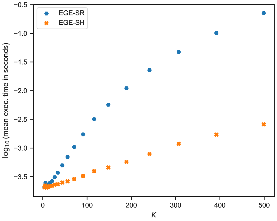
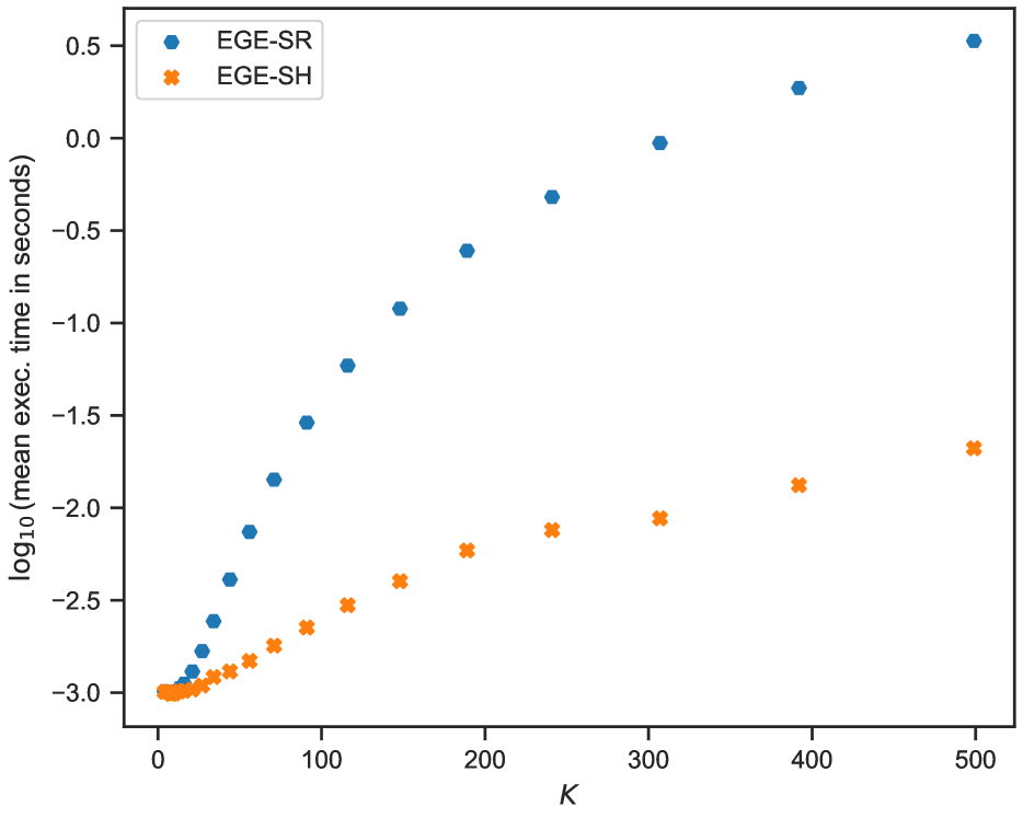
We report below the average runtime of our algorithms for the experiments reported in the main paper. We report on Fig.15 and Fig.15 the runtime versus the number of arms for EGE-SR/SH with varying $K$ and $T=1000$. We average the runtime over 2000 runs. We observe that both algorithms can be used for applications on large scale datasets with a reasonable runtime.

Figure 14: $\log_{10}$ of the mean execution time in seconds averaged over $2000$ trials for an instance with $D=2.$

Figure 15: $\log_{10}$ of the mean execution time in seconds averaged over $2000$ trials for an instance with $D=20.$

G.2 Additional experiments

We report results of additional experiments in particular for the $k$-relaxation. We try different values of $k$ and we compute the loss or mis-identification error averaged over the trials. We plot the average loss versus the budget for each value of $k$. For additional experiments on PSI, the protocol is as described in the main paper.

G.2.1 Experiments on PSI-$k$

We report the experimental result of EGE-SR-$k$ on two bandit instances with a large number of arms. For each bandit instance we test different values of $k$ and we report $\log_{10}$ of the loss averaged over 4000 independent trials. Recall that given $k$ and $T$ the PSI-$k$ loss is

$$\mathcal{L}(\widehat{S}_{T},k):=\begin{cases}\mathbb{I}\{\widehat{S}_{T}\subset\mathcal{S}^{\star}\}&\text{if}\quad\lvert\widehat{S}_{T}\lvert=k,\\ \mathbb{I}\{\widehat{S}_{T}=\mathcal{S}^{\star}\}&\text{else}.\end{cases}$$

Figure 16: Estimated PSI-$k$ loss for different values of $k$ on the SNW dataset.

Figure 17: Estimated PSI-$k$ loss for different values of $k$ on Exp.1 (convex Pareto set)

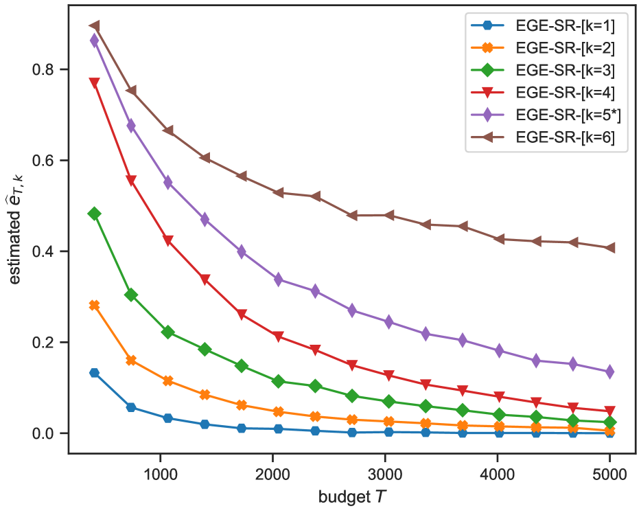
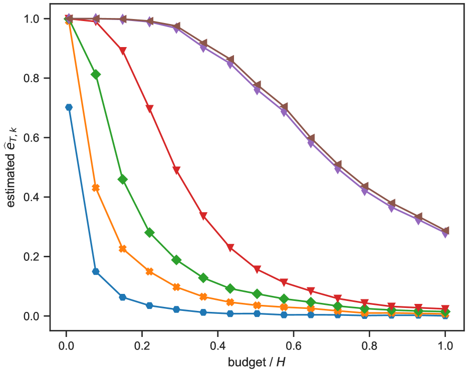
We observe (Fig. 16 and Fig.17) that the loss (the probability of error of EGE-SR-$k$ ​) decreases exponentially fast with the budget. The asterisk indicates the true size of the Pareto set of the instance. We remark that the smaller $k$ the smaller the loss, which is expected as the quantity $H_{2}(\nu)^{(k)}$ (Theorem 3) increases with $k$. We also note that for $k=\lvert\mathcal{S}^{\star}\lvert$, the loss can be smaller than when $k>\lvert\mathcal{S}^{\star}\lvert$. An equivalent remark (in terms of sample complexity) has been made by Kone et al., (2023) for the PSI-$k$ problem in fixed-confidence. Indeed for $k=\lvert\mathcal{S}^{\star}\lvert$ the PSI-$k$ problem is not exactly PSI. As in PSI-$k$ we stop as soon as $k$ optimal arms have been found, in PSI, on the same run, we would continue until all the arms have been classified; thus we could make mistakes on theses additional steps. Finally, note that the expected loss of PSI-$k$ is the same as PSI for any $k>\lvert\mathcal{S}^{\star}\lvert$.

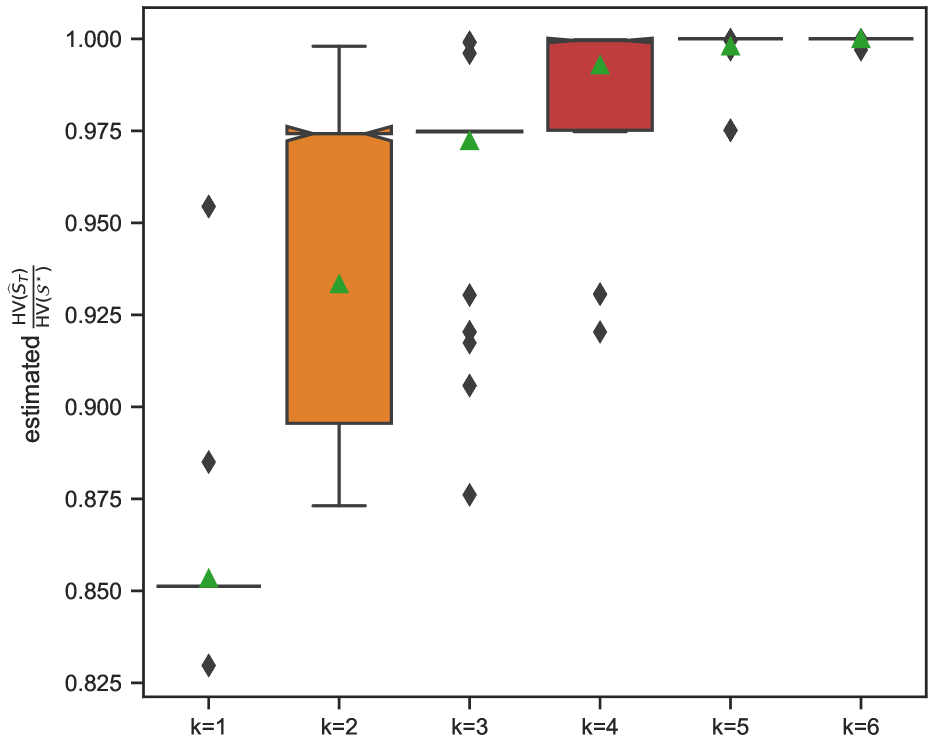
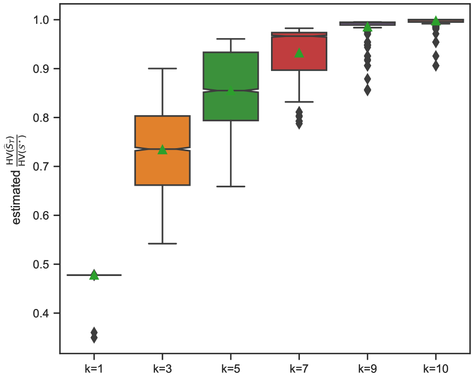
Hyper-volume metric

: The hyper-volume metric (see e.g Daulton et al., (2020)) measures the region dominated by a set of points. Given a reference point $\bm{r}$ and a set $S\subset\mathbb{R}^{D}$ the hyper-volume of $S$ is

$$\text{HV}(S):=\lambda\left(\bigcup_{\bm{x}\in S}[\bm{r},\bm{x}]\right),$$

where $\lambda$ is the Lebesgue measure on $\mathbb{R}^{D}$ and $[\bm{r},\bm{x}]$ is the hyper-rectangle $[r^{1},x^{1}]\times\dots\times[r^{D},x^{D}]$. If $S^{\prime}\subset S$ then $\text{HV}(S)\geq\text{HV}(S^{\prime})$. More importantly, the hyper-volume of $S$ is equal to the hyper-volume of its Pareto set. We use this indicator to measure the quality of the set returned by EGE-SR-$k$ ​. We report the average value of

$$\alpha_{\text{HV}}:=\frac{\text{HV}(\widehat{S}_{T})}{\text{HV}(\mathcal{S}^{\star})}$$

over the trials for different values of $k$ and $T$ fixed. The larger this hyper-volume fraction the more $\widehat{S}_{T}$ covers $\mathcal{S}^{\star}$ in term of dominated region and thus is representative of $\mathcal{S}^{\star}$.

We observe on Fig.18 that the estimated value of $\mathbb{E}[\alpha_{\text{HV}}]$ is nearly $0.85$ for $k=1$ and it naturally increases with $k$. In Fig.19, for $k=1$, the arm returned by EGE-SR-$k$ ​ covers nearly half of the region dominated by the Pareto set. These observations suggest that the arms with the highest hyper-volume contribution are easier to identify as optimal hence they will be the first added to $B_{r}$.

Figure 18: Hyper-volume fraction of the returned set for $T=5000$ on the SNW dataset.

Figure 19: Hyper-volume fraction of the returned set for $T=H$ on Exp.1 (convex Pareto set)

G.2.2 Additional experiments on PSI

We report additional experimental results on 4 synthetic instances which complements our results reported in the main paper. The new instances are described below.

Experiment 5: 2 clusters of arms. We set $K=20$ and we choose $(\bm{\theta}_{1},\dots,\bm{\theta}_{10})\sim\mathcal{U}\left([0.2,0.4]^{2}\right)^{\otimes 10}$ and $(\bm{\theta}_{11},\dots,\bm{\theta}_{20})\sim\mathcal{U}\left([0.5,0.7]^{2}\right)^{\otimes 10}$. There are 4 optimal arms for this instance.

Experiment 6: All the arms are optimal $K=10,D=2$ and for any arm $i$, $\theta_{i}^{1}=0.75-0.65^{i},\theta_{i}^{2}=0.25+0.65^{i}$

Experiment 7: All the arms have the same sub-optimality gap. $K=22,D=2$ and we choose $\bm{\Theta}$ to have $\Delta_{1}=\dots=\Delta_{22}$. Unlike single-objective bandit, such instances can be generated with all arms being different. We choose for $i=1,\dots 8$, $\bm{\theta}_{i}:=(0.3+c_{i},0.8-c_{i})^{\intercal}$ and $c_{i}=(i-1)*c$. For $i=9,\dots,15$, $\bm{\theta}_{i}:=(0.25+c_{i-8},0.7-c_{i-8})^{\intercal}$ and for $i=16,\dots,22$, $\bm{\theta}_{i}:=\bm{\theta}_{i-7}-(0,-0.05)^{\intercal}$.

Experiment 8: Geometric progression with a single optimal arm. We set $K=5,D=2$ and for any $i\in\{1,\dots,5\}$, $\theta_{i}^{1}=\theta_{i}^{2}=0.75-0.25^{i}$. For this instance there is a unique optimal arm.

Figure 20: Synthetic Experiment 5: 2 clusters of arms

Figure 21: Synthetic Experiment 6: All the arms are optimal.

Figure 22: Synthetic Experiment 7: The same gap: $\Delta_{i}=\Delta$ for each arm

Figure 23: Synthetic Experiment 8: Geometric progression

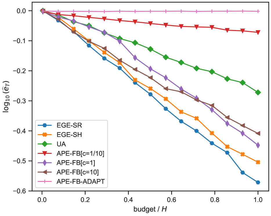
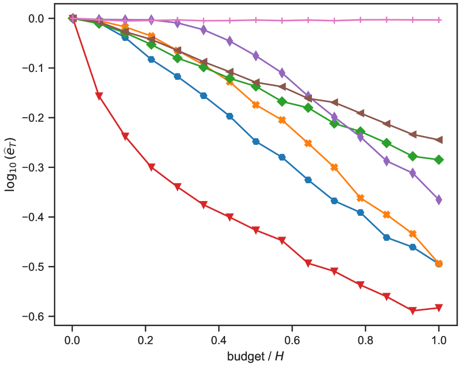
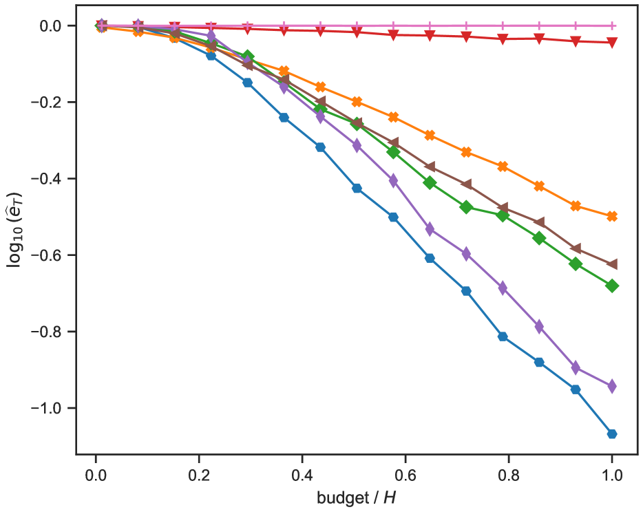
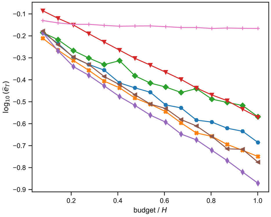
The experiments (Fig.20 to Fig.23) confirm the superior performance of EGE on general instance types. We note however that on experiment 7, where all the arms have the same sub-optimality gaps EGE-SH is slightly outperformed by Uniform allocation but both are largely outperformed by EGE-SR and APE-FB . This is not surprising as on such instances, the exponential decay rate of the mis-identification error of uniform allocation is smaller than that of EGE-SH. Indeed when $\Delta_{1}=\dots=\Delta_{K}$ we have $K\Delta_{(1)}^{-2}=H_{1}(\nu)=H_{2}(\nu)$ thus the result of Table 1 becomes

$$e_{T}^{\text{UA}}(\nu)\leq 2(K-1)\lvert\mathcal{S}^{\star}\lvert D\exp\left(-\frac{T}{144\sigma^{2}H(\nu)}\right),$$

which is even tighter than APE-FB when $T$ is larger than $\lvert\mathcal{S}^{\star}\lvert$. For BAI (PSI with $D=1$), it is know (Audibert and Bubeck,, 2010) that on instances where the gaps are all the same, the uniform allocation is optimal. For example, by taking $\theta_{1}=0.7$ and $\theta_{i}=0.4$ for $i=2,\dots,8$ and a Bernoulli, the gaps are all the same on this instance and one can observe empirically that the Uniform allocation slightly outperforms Sequential Halving (Karnin et al.,, 2013) on this instance.

References

- Ararat and Tekin, (2023) Ararat, C. and Tekin, C. (2023). Vector optimization with stochastic bandit feedback. In Proceedings of The 26th International Conference on Artificial Intelligence and Statistics, pages 2165–2190. PMLR.
- Atsidakou et al., (2023) Atsidakou, A., Katariya, S., Sanghavi, S., and Kveton, B. (2023). Bayesian fixed-budget best-arm identification. arXiv preprint, eprint:2211.08572.
- Audibert and Bubeck, (2010) Audibert, J.-Y. and Bubeck, S. (2010). Best arm identification in multi-armed bandits. In COLT - 23th Conference on Learning Theory - 2010.
- Auer et al., (2016) Auer, P., Chiang, C.-K., Ortner, R., and Drugan, M.-M. (2016). Pareto front identification from stochastic bandit feedback. In Proceedings of the 19th International Conference on Artificial Intelligence and Statistics, pages 939–947. PMLR.
- Bubeck et al., (2013) Bubeck, S., Wang, T., and Viswanathan, N. (2013). Multiple identifications in multi-armed bandits. In Proceedings of the 30th International Conference on Machine Learning, pages 258–265. PMLR.
- Carpentier and Locatelli, (2016) Carpentier, A. and Locatelli, A. (2016). Tight (lower) bounds for the fixed budget best arm identification bandit problem. In 29th Annual Conference on Learning Theory, Proceedings of Machine Learning Research, pages 590–604. PMLR.
- Daulton et al., (2020) Daulton, S., Balandat, M., and Bakshy, E. (2020). Differentiable expected hypervolume improvement for parallel multi-objective bayesian optimization. In Proceedings of the 34th International Conference on Neural Information Processing Systems. Curran Associates Inc.
- Deb et al., (2002) Deb, K., Pratap, A., Agarwal, S., and Meyarivan, T. (2002). A fast and elitist multiobjective genetic algorithm: Nsga-ii. IEEE Transactions on Evolutionary Computation, pages 182–197.
- Degenne, (2023) Degenne, R. (2023). On the existence of a complexity in fixed budget bandit identification. In Proceedings of Thirty Sixth Conference on Learning Theory, Proceedings of Machine Learning Research, pages 1131–1154. PMLR.
- Drugan and Nowe, (2013) Drugan, M.-M. and Nowe, A. (2013). Designing multi-objective multi-armed bandits algorithms: A study. In The 2013 International Joint Conference on Neural Networks (IJCNN), pages 1–8.
- Even-Dar et al., (2002) Even-Dar, E., Mannor, S., and Mansour, Y. (2002). Pac bounds for multi-armed bandit and markov decision processes. In Annual Conference Computational Learning Theory.
- Faizal and Nair, (2022) Faizal, F. Z. and Nair, J. (2022). Constrained pure exploration multi-armed bandits with a fixed budget.
- Gabillon et al., (2012) Gabillon, V., Ghavamzadeh, M., and Lazaric, A. (2012). Best arm identification: A unified approach to fixed budget and fixed confidence. In Advances in Neural Information Processing Systems. Curran Associates, Inc.
- Garivier and Kaufmann, (2016) Garivier, A. and Kaufmann, E. (2016). Optimal best arm identification with fixed confidence. In 29th Annual Conference on Learning Theory, pages 998–1027. PMLR.
- Jamieson et al., (2014) Jamieson, K., Malloy, M., Nowak, R., and Bubeck, S. (2014). lil’ ucb : An optimal exploration algorithm for multi-armed bandits. In Proceedings of The 27th Conference on Learning Theory, pages 423–439. PMLR.
- Jourdan et al., (2023) Jourdan, M., Degenne, R., and Kaufmann, E. (2023). An -best-arm identification algorithm for fixed-confidence and beyond. Thirty-Seventh Conference on Neural Information Processing Systems.
- Kalyanakrishnan et al., (2012) Kalyanakrishnan, S., Tewari, A., Auer, P., and Stone, P. (2012). PAC subset selection in stochastic multi-armed bandits. In Proceedings of the 29th International Coference on International Conference on Machine Learning, pages 227–234. Omnipress.
- Karnin et al., (2013) Karnin, Z., Koren, T., and Somekh, O. (2013). Almost optimal exploration in multi-armed bandits. In Proceedings of the 30th International Conference on International Conference on Machine Learning. JMLR.
- Karpov and Zhang, (2022) Karpov, N. and Zhang, Q. (2022). Collaborative best arm identification with limited communication on non-iid data. arXiv preprint, eprint:2207.08015.
- Katz-Samuels and Scott, (2018) Katz-Samuels, J. and Scott, C. (2018). Feasible arm identification. In Proceedings of the 35th International Conference on Machine Learning, pages 2535–2543. PMLR.
- Katz-Samuels and Scott, (2019) Katz-Samuels, J. and Scott, C. (2019). Top feasible arm identification. In Proceedings of the Twenty-Second International Conference on Artificial Intelligence and Statistics, pages 1593–1601. PMLR.
- Kaufmann et al., (2016) Kaufmann, E., Cappé, O., and Garivier, A. (2016). On the complexity of best-arm identification in multi-armed bandit models. Journal of Machine Learning Research, 17(1):1–42.
- Knowles, (2006) Knowles, J. (2006). Parego: a hybrid algorithm with on-line landscape approximation for expensive multiobjective optimization problems. IEEE Transactions on Evolutionary Computation, pages 50–66.
- Kone et al., (2023) Kone, C., Kaufmann, E., and Richert, L. (2023). Adaptive algorithms for relaxed pareto set identification. In Thirty-seventh Conference on Neural Information Processing Systems.
- Lattimore and CSzepesvári, (2020) Lattimore, T. and CSzepesvári, C. (2020). Bandit Algorithms. Cambridge University Press.
- Locatelli et al., (2016) Locatelli, A., Gutzeit, M., and Carpentier, A. (2016). An optimal algorithm for the thresholding bandit problem. In Proceedings of The 33rd International Conference on Machine Learning, Proceedings of Machine Learning Research, pages 1690–1698. PMLR.
- Munro et al., (2021) Munro, A.-P.-S., Janani, L., Cornelius, V., and et al. (2021). Safety and immunogenicity of seven COVID-19 vaccines as a third dose (booster) following two doses of ChAdOx1 nCov-19 or BNT162b2 in the UK (COV-BOOST): a blinded, multicentre, randomised, controlled, phase 2 trial. The Lancet, 398(10318):2258–2276.
- You et al., (2023) You, W., Qin, C., Wang, Z., and Yang, S. (2023). Information-directed selection for top-two algorithms. In Proceedings of Thirty Sixth Conference on Learning Theory, Proceedings of Machine Learning Research, pages 2850–2851. PMLR.
- Zuluaga et al., (2016) Zuluaga, M., Krause, A., and Püschel, M. (2016). e-pal: An active learning approach to the multi-objective optimization problem. Journal of Machine Learning Research, 17(104):1–32.
- Zuluaga et al., (2012) Zuluaga, M., Milder, P., and Püschel, M. (2012). Computer generation of streaming sorting networks. In DAC Design Automation Conference 2012, pages 1241–1249.
- Zuluaga et al., (2013) Zuluaga, M., Sergent, G., Krause, A., and Püschel, M. (2013). Active learning for multi-objective optimization. In Proceedings of the 30th International Conference on Machine Learning, volume 28, pages 462–470. PMLR.