Learned Causal Method Prediction

Abstract

For a given causal question, it is important to efficiently decide which causal inference method to use for a given dataset. This is challenging because causal methods typically rely on complex and difficult-to-verify assumptions, and cross-validation is not applicable since ground truth causal quantities are unobserved. In this work, we propose CAusal Method Predictor (CAMP), a framework for predicting the best method for a given dataset. To this end, we generate datasets from a diverse set of synthetic causal models, score the candidate methods, and train a model to directly predict the highest-scoring method for that dataset. Next, by formulating a self-supervised pre-training objective centered on dataset assumptions relevant for causal inference, we significantly reduce the need for costly labeled data and enhance training efficiency. Our strategy learns to map implicit dataset properties to the best method in a data-driven manner. In our experiments, we focus on method prediction for causal discovery. CAMP outperforms selecting any individual candidate method and demonstrates promising generalization to unseen semi-synthetic and real-world benchmarks.

1 Introduction

Causal models are needed across diverse application domains as they can be used to understand the underlying mechanisms behind the data and the consequences of unseen interventions. While there has been sustained progress in causal inference and discovery (Yao et al., 2021; Squires and Uhler, 2022), the effective application of causal methods to a given dataset often requires a deep understanding of the available methods and their compatibility with the problem at hand. Such barriers to entry can preclude the widespread adoption of causal inference methods.

An exciting prospect is instructing transformer-based Large Language Models (LLMs) to perform causal tasks, thereby granting a natural language interface for causal inference. A number of emergent abilities have been observed (Wei et al., 2022) including some general reasoning abilities (Bubeck et al., 2023). Unfortunately, while LLMs are able to exploit domain knowledge relevant for causal inference (Kıcıman et al., 2023; Long et al., 2023), their ability to perform advanced causal reasoning is still limited (Zhang et al., 2023; Zevcević et al., 2023). Furthermore, improving causal capabilities of LLMs with fine-tuning strategies, like instruction fine-tuning (Ouyang et al., 2022), may prove infeasible as soliciting labels requires expensive controlled experiments. Nevertheless, existing LLMs have proven to be remarkably extensible by using external tools (Chase, 2022; Schick et al., 2023). Zhang et al. (2023) propose following this line to augment LLMs with causal reasoning. However, similar to practitioners, LLMs incorporating causal tools require a strategy for choosing the appropriate causal method for a particular problem.

We refer to causal method selection as the task of choosing the best method for a given causal task from a candidate set $\{M_{1},M_{2},\ldots,M_{K}\}$ for a given dataset $D_{n}$. For example, if the causal task is structure learning, then the methods would be various causal discovery algorithms. Our goal in this work is to efficiently select the best method for the given causal task from the input dataset. The selection problem is especially challenging in the causal setting. Causal inference relies on strong assumptions. Many such assumptions, like causal sufficiency, are inherently untestable (Ashman et al., 2023; Kong et al., 2023). Even with domain knowledge justifying these assumptions, multiple methods might be available. Techniques like cross-validation do not apply since evaluation depends on the true Structural Causal Model (SCM). However, many assumptions, such as linear or normality, are testable in principle (Mohd Razali and Yap, 2011). Thus, observable features of a dataset can be used to guide the choice of the best causal method. One can pick the most generally applicable method available, however, simpler methods might work better due to a limited sample size or fewer tuning parameters. Moreover, beyond explicit assumptions, the performance of a causal method also depends on implicit dataset properties and optimization concerns.

In this work, inspired by foundation models (Bommasani et al., 2021), we propose CAMP, a framework for learning the best method for a given dataset (Sec. 4) in a supervised manner. Our work builds on prior supervised approaches for predicting the causal structure from an input dataset (Ke et al., 2022; Lorch et al., 2022). We generate datasets from a diverse set of synthetic SCMs, score all candidate methods on every dataset, and then train a model to directly predict the best method for an input dataset. Unlike traditional supervised learning, we make one prediction per dataset and not per sample. Given that knowledge of the underlying dataset properties like linearity can aid method selection, we formulate a self-supervised pre-training objective around predicting the dataset assumptions (Sec. 4.2), and then fine-tune the pre-trained model on a limited labeled data. The self-supervision provides a simple and effective way to inject useful inductive biases into the model, improves computational efficiency, requiring lesser labeled data as well as fewer training iterations.

Our approach allows learning implicit dataset features to predict which method is best for a dataset. This may include, but is not limited to testable assumptions made by the different methods. At inference time, CAMP can provide fast zero-shot predictions of the best method for a dataset. Additionally, CAMP can be applied to a wide range of causal tasks such as causal discovery, treatment effect estimation, and covariate selection, where the labels can be generated using synthetic SCMs. In our experiments, we focus on the task of method selection for causal discovery (Sec. 5). We observe that, despite being trained on only synthetic data, CAMP generalizes to synthetic out-of-distribution datasets and performs well on semi-synthetic and real-world gene expression benchmarks, outperforming simple heuristics for method selection like selecting the best method on average.

2 Related Work

Non-Causal Model Selection

Our work is related to model selection which has been studied by many works in the context of supervised machine learning. The common techniques are the holdout validation method and $k$-fold cross-validation, both of which use one partition of the data for training and a different one for evaluation (Raschka, 2018; Arlot and Celisse, 2010). The field of Automated machine learning (AutoML) aims to automate various parts of the machine learning pipeline like feature and hyperparameter selection aiming to reduce human effort in designing these pipelines (He et al., 2021; Hutter et al., 2019). These methods do not directly apply in the causal setting since evaluation requires knowledge of the true causal model, such as the true graph or counterfactual data, which are not known for real problems.

Evaluating Causal Methods

Another line of work studies model evaluation and selection for causal inference. For conditional average treatment effect (CATE) estimation, many works have proposed data-driven strategies for model selection based on estimates of the counterfactual risk (Rolling and Yang, 2014; Gutierrez and Gérardy, 2017; Alaa and Van Der Schaar, 2019; Saito and Yasui, 2020). Empirical studies comparing numerous estimators and model selection strategies for CATE estimation have also been conducted revealing complex interactions between the underlying data assumptions, methods, and selection strategies (Schuler et al., 2018; Mahajan et al., 2022; Machlanski et al., 2023; Curth and van der Schaar, 2023; Matthieu and Gaël, 2023). For model selection and hyperparameter tuning in causal discovery, various metrics have been used like the stability of the output across dataset perturbations (Liu et al., 2010; Raghu et al., 2018) and multiple runs (Strobl, 2021), the Bayesian Information Criterion (Maathuis et al., 2009, Sec. 4.1), predictive performance of the learned causal model (Biza et al., 2020, 2022), and compatibility of the learned graphs across different subsets of variables (Faller et al., 2023). In contrast, we take a supervised learning approach to predict the best causal method and our strategy can be viewed as complementary to these works.

Supervised Causal Inference

A closely related line of work frames causal discovery as a supervised learning task. Li et al. (2020) study supervised causal discovery using synthetic datasets for linear causal models, predicting the causal graph from an input correlation matrix. Petersen et al. (2022) propose to learn an equivalence class of causal graphs from an observational dataset by training on simulated linear Gaussian data. Ke et al. (2022) propose a transformer-based model that learns to map a dataset with observational and interventional samples to the causal structure in a supervised manner using synthetic training data. Ke et al. (2023) extend this work for discovering gene regularity networks. Wang and Kording (2022) propose a supervised causal discovery method for synthetic microprocessor and brain-network datasets. Lorch et al. (2022) propose AVICI, a variational inference model to predict the causal structure directly from the input dataset, training on synthetically generated datasets. We use the self-attention architecture of AVICI to make dataset-level predictions. The architecture encodes desirable permutation invariances for improving the statistical efficiency of the predictor. While these works predict the causal structure in a supervised manner, they do not consider method selection.

3 Problem Formulation

Method	Description
DirectLiNGAM (Shimizu et al., 2011)	DAG learning for linear non-Gaussian data
NOTEARS-linear (Zheng et al., 2018)	A gradient-based method for linear data
NOTEARS-MLP (Zheng et al., 2020)	MLP-based NOTEARS for nonlinear data
DAG-GNN (Yu et al., 2019)	DAG learning with Graph Neural Networks
GraNDAG (Lachapelle et al., 2019)	DNN-based method for nonlinear additive noise data
DECI (Geffner et al., 2022)	Bayesian method for nonlinear additive noise data

Table 1: Brief description of the six candidate causal discovery methods.

In this work, given a dataset ${\bf X}$, the aim is to choose the best causal method (as assessed by some score function) from a candidate set $\{M_{1},M_{2},\ldots,M_{K}\}$ at test time. The dataset is denoted as ${\bf X}\in{\mathbb{R}}^{n\times V}$, where $n$ is the number of samples and $V$ is the number of variables (we assume real-valued data but our approach can be generalized to discrete and mixed-type datasets). There is a set of $K$ candidate methods: ${\mathcal{M}}=\{M_{1},\ldots,M_{K}\}$ and a scoring function $s(M,{\bf X};\theta_{*})\in{\mathbb{R}}$ for method $M\in{\mathcal{M}}$ and dataset ${\bf X}$ that depends on some features of the true SCM (e.g., the true graph), denoted by $\theta_{*}$. The goal is to develop a selection strategy ${\mathcal{S}}:{\mathbb{R}}^{n\times V}\mapsto{\mathcal{M}}$ such that the selected method ${\mathcal{S}}({\bf X})$ maximizes the score $s({\mathcal{S}}({\bf X}),{\bf X};\theta_{*})$. The score function determines how the methods are assessed for the problem at hand. In the causal inference setting, this score cannot be estimated using a holdout validation set since it depends on the unknown true causal model.

Throughout, we assume that the $n$ samples are generated i.i.d. from (unknown) SCM associated with a directed acyclic graph (DAG) $G_{*}$ over $V$ nodes (Peters et al., 2017, Sec. 6.2). Each node $X_{j}$, for $j\in[V]$, is generated according to the structural equation $X_{j}:=f_{j}(X_{\text{pa}(j;G_{*})},n_{j})$, where $n_{j}$ is an exogenous noise term, $\text{pa}(j;G_{*})$ denotes the parents of $X_{j}$ in $G_{*}$, and $f_{i}$ is an arbitrary function describing how $X_{j}$ depends on its parents and the noise term.

In this work, we focus on method selection for causal discovery from observational data. In causal discovery, the aim is to discover the underlying causal graph (or equivalence class thereof) from the dataset ${\bf X}$. We consider six candidate causal discovery methods: ${\mathcal{M}}=\{$ DirectLiNGAM (Shimizu et al., 2011), NOTEARS-linear (Zheng et al., 2018), NOTEARS-MLP (Zheng et al., 2020), DAG-GNN (Yu et al., 2019), GraNDAG (Lachapelle et al., 2019), and DECI (Geffner et al., 2022) $\}$. Every method $M\in{\mathcal{M}}$ outputs an estimated DAG $\widehat{G}_{M}({\bf X})$. These methods work with observational data and assume causal sufficiency (i.e., no hidden variables), which also entails that each noise term $n_{j}$ is independent of all other variables. The candidate set ${\mathcal{M}}$ was chosen to encompass methods for linear and nonlinear SCMs as well as recent gradient and neural network-based methods (see Table 1 for a brief description of the methods).

We use the F1-score between the binary adjacency matrices of the true DAG and the estimated DAG as the scoring function for evaluating the causal discovery methods: $s(M,{\bf X};G_{*})=\text{F1}(\widehat{G}_{M}({\bf X}),G_{*})$. The F1-score is a commonly used metric for evaluating the performance of causal discovery algorithms and its range is agnostic to the size of the graph (unlike structural hamming distance), enabling meaningfully comparisons of the scores across different graph sizes.

4 Learned Causal Method Prediction

Figure 1: An illustration of an interaction with an LLM augmented with CAMP. The LLM can parse the user’s intent from their natural language query and invoke CAMP to answer causal questions, allowing the practitioner to interact with causal methods effortlessly.

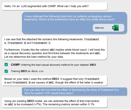
In this section, we describe CAusal Method Predictor (CAMP), a framework for learning the mapping from a dataset to the best method. We describe two strategies for predicting the best method: (i) Supervised (Sec. 4.1): we train a deep neural network (DNN) to directly classify the highest-scoring method from the input dataset; and (ii) Semi-supervised (Sec. 4.2): we propose a self-supervision strategy to pre-train the DNN before fine-tuning it on labeled data, improving the statistical and computational efficiency of the purely supervised approach. The supervision allows CAMP to learn observable features of the input dataset (beyond explicitly specified assumptions) that can be used to decide the best causal method in a data-driven manner.

CAMP can be readily integrated with an LLM to form an augmented causal agent that can answer causal questions from a given dataset (see Fig. 1 for a demonstration of this interaction mode with such an agent). For a natural language query, the LLM can parse the user’s intent to determine the causal task they want to perform (e.g., causal discovery), and invoke CAMP as an external tool to determine the best causal method for that dataset and causal task.

4.1 Supervised Causal Method Predictor (CAMP-Sup)

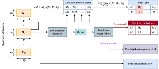
We treat causal method selection as as a $K$-class classification task. We generate labeled training data consisting of $({\bf X},L)$ instances, where ${\bf X}$ is a dataset and $L\in{\mathcal{M}}$ is the target candidate method, and train a DNN to predict the target label $L$ from the input dataset ${\bf X}$. Unlike traditional supervised learning, we make one prediction per dataset (not per sample).

Training data.

We generate the training instances as follows: (i) we sample a random SCM (see Sec. 5.1 for details on the sampling) and generate a dataset ${\bf X}\in{\mathbb{R}}^{n\times V}$ from that SCM with random $n$ and $V$; (ii) we run each candidate method on the dataset ${\bf X}$ and score it using the true graph $G_{*}$ (which is known since the SCM is synthetic); and (iii) the target label $L$ is the method with the highest score: $L=\arg\max_{M\in{\mathcal{M}}}s(M,{\bf X})$. The full training data is $(X_{i},\,L_{i})_{i=1}^{T}$.

Model architecture.

We use an encoder-decoder-style model. The encoder takes the input dataset $\mathbf{X}\in\mathbb{R}^{n\times V}$ (with arbitrary $n$ and $V$) and outputs a $Z$-dimensional embedding of the dataset. We use the same encoder architecture as (Lorch et al., 2022, Sec. 4.2). The encoder is composed of $L$ identical layers. The crux of each layer is an alternating multi-headed self-attention: the first self-attention attends across the $V$ axis, treating $n$ as the batch dimension; the second self-attention attends across the $n$ axis, treating $V$ as the batch dimension. After $L$ such layers, the output dimension is $(n\times V\times Z)$, where $Z$ is the embedding dimension of the muli-headed self-attention. The attention layers allow the network to aggregate information across both the sample and node axes as well as process an arbitrary-sized dataset. Similar to Lorch et al. (2022), we then apply a max-pooling across the $n$ and $V$ axes, resulting in a $Z$-dimensional dataset embedding. This embedding is permutation invariant across both the $n$ and $V$ axes: this is desirable because the prediction should be agnostic to the order of the samples (since they are i.i.d.) and the nodes. The decoder is a fully-connected feedforward network (FFN) with a $K$-dimensional output representing the classification logits for each of the candidate methods. Although we use the same DNN architecture as Lorch et al. (2022), our goal is to predict the best method. In contrast, they attempt to learn the DAG directly in a supervised manner and in principle, their method AVICI can be added to the list of candidate methods that we select among.

Loss function.

We treat method selection as a multi-class classification problem and train the DNN end-to-end with the cross-entropy loss:

$$L_{\text{CE}}(p,L)=-\sum_{i=1}^{K}L_{i}\log(p_{i}),$$ (1)

where $p\in\Delta^{K-1}$ are the predicted probabilities and $L\in\{0,1\}^{K}$ is the one-hot vector denoting the target label. Since we also have access to the raw scores of all candidate methods for each dataset, rank-based loss functions can also be used (Wang et al., 2018). Empirically, we did not see an improvement with these loss functions and so we used the cross-entropy loss in our experiments (see Fig. 7 in Appendix B).

Figure 2: Training pipelines for CAMP-Sup and CAMP-SemiSup. For CAMP-Sup, we generate synthetic datasets, score each candidate, and classify the highest-scoring method. For CAMP-SemiSup, there is a self-supervised pre-training step to predict the SCM assumptions, followed by supervised fine-tuning on a limited amount of labeled data.

Inference.

At inference time, we perform a forward pass through the trained DNN to get the best method for the input dataset. The supervised approach enables zero-shot prediction of the best method, which is fast, because we do not need to run all candidate methods at inference time. The model learns a mapping from implicit dataset features to the best method in a data-driven manner.

4.2 Semi-Supervised Causal Method Predictor (CAMP-SemiSup)

Generating labels can be computationally expensive because it requires running all candidate methods on every dataset. This is especially problematic in the case of causal discovery where running even a single method can take a long time. Addressing this concern, we propose a semi-supervised approach based on self-supervised pre-training followed by supervised fine-tuning (Zhai et al., 2019; Chen et al., 2020).

Inferring causality from observational data always requires some assumptions on the data-generating process. In causal discovery, different methods utilize different sets of assumptions on the SCM and knowledge of these assumptions can be informative in determining the best method. So we formulate a self-supervised pre-training objective around predicting the assumptions that hold in the underlying causal model that are relevant to the causal task at hand (e.g., whether linearity or normality holds). This injects useful inductive biases into the DNN prior to the supervised finetuning step.

Let $\Theta$ denote some set of SCMs and ${\mathcal{A}}$ denote some set of (testable) assumptions of an SCM. Consider a function $a:\Theta\mapsto{\mathcal{A}}$ that maps an SCM to the assumptions that hold for that SCM. The set ${\mathcal{A}}$ can represent any assumptions that might be useful for selecting among the candidate methods. For synthetically constructed SCM and dataset pairs $(\theta_{i},{\bf X}_{i})_{i=1}^{T}$, where $\theta_{i}\in\Theta$ and ${\bf X}_{i}$ is generated from SCM $\theta_{i}$, we train an encoder-decoder DNN similar to Sec. 4.1 to predict $a(\theta_{i})$ from the input dataset ${\bf X}_{i}$. Generating training data for this self-supervised task is relatively cheap: $a(\theta_{i})$ can directly be determined from the synthetic SCM $\theta_{i}$ without running any of the candidate methods. After training this DNN, we take this pre-trained encoder and fine-tune it on limited labeled data as described in Sec. 4.1. For our experiments, we use ${\mathcal{A}}=\{\text{Linear Gaussian},\text{Linear non-Gaussian},\text{Nonlinear}\}$. Since ${\mathcal{A}}$ is a discrete set in our experiments, we treat it as a $3$-way classification task and use the cross-entropy loss for pre-training.

In practice, the space ${\mathcal{A}}$ can contain other properties of an SCM that can be useful for determining the best causal method, like the presence and type of identifiable unmeasured confounders (e.g., bow-free confounding (Ashman et al., 2023)), characteristics of the DAG (e.g., sparsity), etc. The set ${\mathcal{A}}$ should be chosen depending on the causal task as well as the candidate methods (Berrevoets et al. (2023) discuss several axes for grouping assumptions for causal inference). In our experiments, we show that the semi-supervised model not only requires lesser labeled data and training steps, but also generalizes better beyond the training distribution. Thus, semi-supervision can also be useful for scaling up the supervised approach to a larger set of methods.

Remark.

One strategy for method selection is to leverage the prediction of the set $a(\theta)$ by mapping each item in ${\mathcal{A}}$ to a method. Our approach is more flexible since we learn this mapping in a data-driven way. Moreover, during supervision, our approach can also learn to use dataset features that might be difficult to explicitly elicit in the space ${\mathcal{A}}$.

5 Experimental Results

We evaluate our causal method selection strategy for synthetic datasets (Sec. 5.2)—both in-distribution and out-of-distribution—as well as four semi-synthetic and real-world benchmark datasets (Sec. 5.3).

5.1 Synthetic training data generation

SCM and dataset generation.

We generate datasets with varying sample and graph sizes from a diverse set of linear and nonlinear SCMs. We consider sample sizes $n\in[600,1200]$ and graph sizes $V\in[8,12]$. The graph is sampled from an Erdos-Renyi distribution with edge probabilities uniformly sampled from $[0.3,0.7]$. We consider a diverse set of SCMs that encompass several linear and nonlinear SCMs considered in the causal discovery literature. Our training data contains datasets from the following causal models: (1) Linear Gaussian: We simulate $X_{j}=w^{\top}_{j}X_{\text{pa}(j)}+n_{j}$, where the coefficients $w_{j}$ are uniformly random and $n_{j}$ is Gaussian (similar to Zheng et al. (2018)); (2) Linear non-Gaussian: The same as Linear Gaussian, but with $n_{j}$ belonging to a uniform or exponential distribution; (3) Nonlinear Additive Noise Models (ANM): We simulate $X_{j}=f_{j}(X_{\text{pa}(j)})+n_{j}$, where $n_{j}$ is Gaussian and each $f_{j}$ is one of two nonlinear functions (similar to Zheng et al. (2020)): (i) random function from a Gaussian Process (GP), or (ii) (Additive GP) $f_{i}(X_{\text{Pa}(i)})=\sum_{j\in\text{Pa}(i))}g_{j}(X_{j})$, where each $g_{j}$ is a random function from a GP; (4) Post-nonlinear (PNL) model (Zhang and Hyvarinen, 2012): We simulate $X_{j}=f_{j}(g_{j}(X_{\text{pa}(j)}+n_{j}))$ where $g_{i},f_{i}$ are nonlinear functions from one of the following PNL models: (i) $f_{i}$ and $g_{i}$ are sampled as weighted sums of GPs and sigmoids (Uemura et al., 2022), or (ii) $f_{i}$ is a polynomial and $g_{i}$ is the cube-root (Keropyan et al., 2023); (5) Location-scale model (Immer et al., 2023): This is a heteroskedastic noise model with $X_{j}=f_{j}(X_{\text{pa}(j)})+g_{j}(X_{\text{pa}(j)})\cdot n_{j}$, where $n_{j}\sim{\mathcal{N}}(0,\sigma^{2}_{j})$ and $f_{j},g_{j}$ are random functions from a GP. The training distribution contains an $\approx 11$–$23$–$66\%$ split of linear non-Gaussian, linear Gaussian, and nonlinear SCMs, respectively; and amongst nonlinear SCMs, we generate each type with equal probability (see Appendix A for additional details on the synthetic data distribution).

Target label.

We consider six causal discovery methods (see Table 1 and Sec. 3). For all methods except DECI, we use the implementations from the library gCastle (Zhang et al., 2021) (we use the default hyperparameters from gCastle for all methods). For DECI, we use the Gaussian noise implementation from the causica package (Kiciman et al., 2022). For each synthetically generated dataset, we run the six causal discovery methods and compute the F1-score using the true DAG. Since DECI is a Bayesian method, we compute the average F1-score across $1000$ draws from its posterior distribution over DAGs. The target label is a one-hot vector denoting the method with the highest F1-score.

Figure 3: Comparison of various strategies for selecting among six causal discovery methods (Table 1) across a diverse set of SCMs (error bars denote 95% CIs). Oracle (Best) chooses the best method for each dataset. The Oracle-LG-NG-NL and Oracle-L-NL oracles select the best method depending on the dataset type, improving over DECI (the best method on average). Both CAMP methods match the score of Oracle-LG-NG-NL.

5.2 Results on synthetic data

We first evaluate the supervised and semi-supervised approaches on a test set with the same distribution as the training set (as described in Sec. 5.1). For the results in this section, we used validation and test sets of $2000$ and $3414$ datasets, respectively. For the encoder, we use $L=4$ layers and attention embedding size $Z=32$; and for the decoder, we used a FFN with $2$ hidden layers of size $32$. For the semi-supervised approach, we used $\approx 50,000$ datasets for the self-supervised pre-training step, and we train the model to predict the underlying SCM assumptions from the set ${\mathcal{A}}=\{\text{Linear Gaussian},\text{Linear non-Gaussian},\text{Nonlinear}\}$. The model achieved a nearly perfect accuracy for this task after the pre-training step.

(a) Labeled data requirements

(b) Rate of convergence

Figure 4: Average F1 scores of CAMP-Sup and CAMP-SemiSup on the test set (errors bars denote standard errors over $4$ runs). CAMP-SemiSup requires (a) lesser training labeled data than CAMP-Sup (with $3000$ labels, CAMP-SemiSup outperforms CAMP-Sup with $6000$ labels); and (b) fewer training steps to converge. For CAMP-SemiSup, $\approx 50,000$ datasets were used for pre-training.

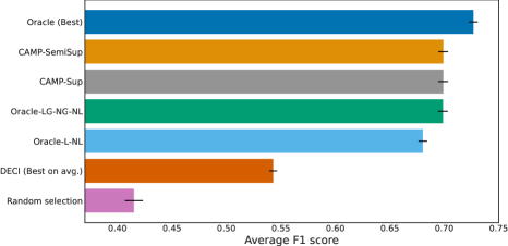
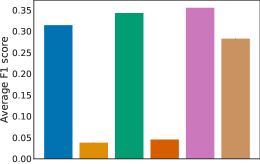
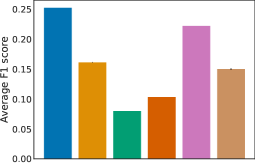
We show the performance of our supervised (CAMP-Sup) and semi-supervised (CAMP-SemiSup) models, trained on $6000$ labeled datasets (see Fig. 3), a test set with the same distribution as the training set. We also plot the following oracles to select the best method: Oracle (Best) selects the best method for every dataset; Oracle-LG-NG-NL selects the best method based on whether the SCM is linear Gaussian, linear non-Gaussian, or nonlinear; and Oracle-L-NL based on whether the SCM is linear or nonlinear (see Fig. 6 in Appendix A for the average F1 scores of the six methods across different SCM types). There is a substantial gap between Oracle (Best) and always picking the best method on average (DECI). As the oracles leverage more knowledge of the dataset properties, their average scores increase relative to DECI with Oracle-LG-NG-NL outperforming Oracle-L-NL. We see that CAMP-Sup and CAMP-SemiSup perform comparably. Both CAMP models significantly outperform always selecting DECI, the best method on average in the training set, as well as the randomly selecting a candidate method (Fig. 3). Next, we observe that CAMP matches the performance of the oracle Oracle-LG-NG-NL. This demonstrates the ability of CAMP to automatically learn the mapping from implicit dataset features to the best method.

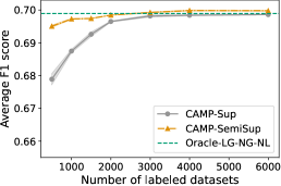
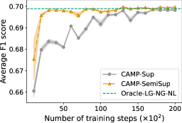
We also compare the average scores of CAMP-Sup and CAMP-SemiSup on the test set across different amounts of labeled training data (see Fig. 4(a)). We observe that both approaches converge to Oracle-LG-NG-NL as the number of training data points gets large. But we see that the CAMP-SemiSup achieves the same average score with fewer labeled data points: $3000$ training datasets suffice for CAMP-SemiSup to match the score of CAMP-Sup with $6000$ labeled datasets. Moreover, the differences in the scores are much larger when the number of labeled data points is small ($<2000$), showing the advantages of the semi-supervised approach in small data regimes. Next, we compare CAMP-Sup and CAMP-SemiSup in terms of how quickly they converge (see Fig. 4(b)). We fix the amount of labeled data points to $6000$ and compare the average scores of the two approaches on the test set across increasing training steps. Although both approaches converge as we train for long enough, CAMP-SemiSup requires significantly fewer training steps: after $\approx 3000$ training steps, it achieves the same score as the CAMP-Sup after $\approx 12000$ steps. These results show the computational and statistical advantages of the semi-supervised approach with a pre-training objective around the SCM assumptions.

Figure 5: Results on synthetic OOD datasets for (a), (b): graphs with a larger number nodes and (c): scale-free graphs. CAMP continues to perform well in regimes (a) and (c). For (b), CAMP still outperforms DECI and Oracle-L-NL.

Out-of-distribution datasets.

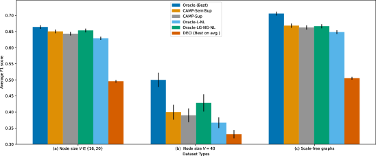
We also test the generalization abilities of our method selection approach beyond the training distribution (see Fig. 5). We evaluate our methods on synthetic SCMs with a larger number of nodes than encountered during training. When we increase the number of nodes to $V\in\{16,20\}$ (Fig. 5a), the model continues to perform well. Further increasing the node size to $V=40$ worsens the performance relative to Oracle (Best) but is still better Oracle-L-NL, with both CAMP models performing worse than the Oracle-LG-NG-NL oracle, showing that much larger graphs can be a challenge for CAMP (Fig. 5b). Next, we test our methods on synthetic datasets generated for scale-free graphs (Barabási and Albert, 1999) (Fig. 5c), showing that the method continues to generalize to a different graph distribution. In all three cases, both CAMP models significantly outperform DECI (the best method on average on the training set).

5.3 Results on semi-synthetic and real-world data

An important concern with supervised training on only synthetic SCMs is the extent to which the selection algorithm generalizes to real-world datasets. Addressing this concern, we demonstrate promising results on the four semi-synthetic and real-world gene expression benchmarks.

We consider the following benchmarks: (i) semi-synthetic datasets generated from the graphs MAGIC-NIAB and MAGIC-IRRI from bnlearn (Scutari, 2010; Scutari et al., 2014); (ii) the SynTReN generator (Van den Bulcke et al., 2006) that creates synthetic gene regulatory networks and simulates gene expression data that approximates experimental data; and the real-world protein cells dataset from Sachs et al. (2005) which is commonly used to benchmark causal discovery algorithms. The MAGIC-NIAB and MAGIC-IRRI are linear Gaussian SCMs with graph sizes $V=44$ and $V=64$, respectively. For both graphs, we sample datasets with $n=1000$ samples, and use the SCM parameters from bnlearn. Both these graphs are significantly larger than the training distribution of CAMP. For SynTReN, we simulate a dataset with $V=20$ nodes and $n=400$ samples. The Sachs et al. (2005) protein cells dataset contains $V=11$ nodes and $n=7466$ samples.

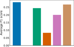
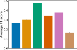
For each of the four benchmark datasets, we first run the six candidate causal discovery methods $10$ times and compute the average F1 score of each method (see Fig. 8 in Appendix C for the F1 scores of the six methods on each benchmark). We compare the true ranking of the six methods on each benchmark against the rankings predicted by CAMP (see Table 2; the complete rankings are in Table 3 in Appendix C). We first compare the scores of the top-ranked methods from CAMP against the true scoring method (Oracle Rank $1$) on each dataset (see Table 2a). We observe that CAMP-SemiSup predicts the best method for all benchmarks except MAGIC-IRRI. In contrast, the best-predicted method from CAMP-Sup performs poorly on the bnlearn graphs (the scores are close to zero because it picks a method that returns a nearly empty graph), but it successfully picks out the best method for SynTReN and the protein cells benchmarks.

	MAGIC-NIAB	MAGIC-IRRI	SynTReN	Protein cells
a) Top-1 F1-score
Oracle	$0.28$	$0.36$	$0.25$	$0.48$
CAMP-SemiSup	0.28	$0.31$	0.25	0.48
CAMP-Sup	$0.00$	$0.02$	0.25	0.48
b) Weighted F1-score
CAMP-SemiSup	0.26	0.32	$0.22$	$0.35$
CAMP-Sup	$0.07$	$0.15$	0.23	0.38
Average score	$0.18$	$0.23$	$0.16$	$0.32$
c) Spearman’s correlation coefficient
CAMP-SemiSup	0.60	0.42	$0.60$	0.54
CAMP-Sup	$-0.37$	$-0.77$	0.71	$0.31$

Table 2: F1 scores of the predicted top-1 method, the average of all methods weighed by their predicted probabilities, and the Spearman correlation between the true and predicted ranks. We see that CAMP-SemiSup performs well across all four benchmarks.

Both CAMP-Sup and CAMP-SemiSup output a vector $p\in\Delta^{K-1}$ (probability simplex), denoting the predicted probability of each method. We compare the average score weighted by this probability: $\sum_{i=1}^{K}p_{i}s(M_{i},{\bf X})$, to the average score with equal weight given to each method (Average score): $\sum_{i=1}^{K}\frac{1}{|{\mathcal{M}}|}s(M_{i},{\bf X})$ (see Table 2b). We observe that CAMP-SemiSup always outperforms the Average score baseline for all benchmarks, and CAMP-Sup is worse on the bnlearn graphs but significantly better for both SynTReN and the protein cells dataset.

Next, we present the Spearman’s correlation coefficient, a measure of agreement between the true ranking of the methods and the ranking determined by their predicted probabilities (see Table 2c). Again, we see that the rankings of CAMP-SemiSup are always positively correlated whereas CAMP-Sup leads to poor results on the bnlearn graphs.

Overall, these results show that CAMP-SemiSup performs well on these benchmarks and selecting the best predicted method leads to a good F1-score. This shows that CAMP may generalize to unseen real-world distributions despite having been trained only on synthetic data. As for the good scores of CAMP-SemiSup on the bnlearn graphs (where CAMP-Sup fails), we conjecture that it is due to the pre-trained inductive biases: the assumption predictor trained during the pre-training step correctly predicts that both bnlearn graphs are linear Gaussian, which potentially allows CAMP-SemiSup to perform much better than CAMP-Sup. This demonstrates that semi-supervision leads to better generalization in practice than the purely supervised approach.

6 Discussion

We leverage large-scale predictive models to select the best causal method by framing the selection problem as a (semi) supervised learning task. We generate datasets from a diverse set of synthetic SCMs and train a model to directly predict the best method from the input dataset. Using synthetic SCMs allows us to construct a large amount of labeled training data. Our experimental results show that CAMP performs favorably against several oracles and shows promising generalization beyond the training distribution on common causal discovery benchmark datasets. Moreover, CAMP can be integrated into an an LLM toolchain to allow users to ask causal questions about their datasets.

Although our experiments focus on method selection for causal discovery, our proposed strategy is more generally applicable. In future work, we hope to test our selection strategy on other causal tasks like treatment effect estimation and covariate selection. Moreover, theoretically understanding the generalization abilities and limits of the supervised approach for causal tasks is also a promising future direction. Beyond causality, we hope to inspire other areas that may benefit from data-driven supervised method selection. For example, one such area is ODE solvers, where factors like problem stiffness may determine which method performs best (Postawa et al., 2020; Dallas et al., 2017). More broadly, our approach can be applied to tasks where there are several candidate methods, and synthetically generated datasets can be used to generate labeled data for learning the mapping from a dataset to the best method.

Appendix A Additional details on synthetic data generation

(a) All Datasets

(b) Linear Gaussian datasets

(c) Linear non-Gaussian datasets

(d) Nonlinear datasets

Figure 6: The average F1 scores (error bars denote 95% CIs) of the six causal discovery methods on synthetic data across (a) All datasets, and (b)-(d) different subsets of the data sliced according to the underlying assumptions.

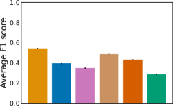
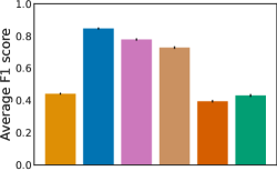
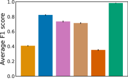
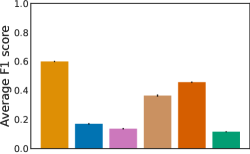
In this section, we provide additional details on the data-generating processes (DGP) for the synthetic datasets (see Sec. 5.1). Throughout, the graphs are sampled from an Erdos-Renyi distribution with the edge probabilities uniformly sampled from $[0.3,0.7]$. Recall that each node $X_{j}$ is generated via the structural equation $X_{j}:=f_{j}(X_{\text{pa}(j;G_{*})},n_{j})$, where $n_{j}$ is an exogenous noise term. Unless stated otherwise, we use Gaussian noise with random variance: $n_{j}\sim{\mathcal{N}}(0,\sigma^{2}_{j})$ where $\sigma_{j}\sim\text{Uniform}([0.2,2])$. We randomly generate the following SCMs:

1. Linear Gaussian: We simulate $X_{j}=w^{\top}_{j}X_{\text{pa}(j)}+n_{j}$, where the coefficients $w_{j}\sim\\ \text{Uniform}([-2,-0.5]\cup[0.5,2])$ (similar to Zheng et al. [2018]).

2. Linear non-Gaussian: This is the same as Linear Gaussian but the noise $n_{j}$ has a uniform or exponential distribution. Amongst the linear non-Gaussian SCMs, we use a $50$–$50\%$ split between uniformly and exponentially distributed noise.

3. Nonlinear Additive Noise Models (ANM) [Peters et al., 2014]: We simulate $X_{j}=f_{j}(X_{\text{pa}(j)})+n_{j}$, where $n_{j}$ is Gaussian and each $f_{j}$ is one of two nonlinear functions (similar to Zheng et al. [2020]): (i) random function from a Gaussian Process (GP), or (ii) (Additive GP) $f_{i}(X_{\text{Pa}(i)})=\sum_{j\in\text{Pa}(i))}g_{j}(X_{j})$, where each $g_{j}$ is a random function from a GP. In both cases, we use a GP with an RBF kernel with scale $1$.

4. Post-nonlinear (PNL) model [Zhang and Hyvarinen, 2012]: We simulate $X_{j}=f_{j}(g_{j}(X_{\text{pa}(j)}+n_{j}))$ where $g_{i},f_{i}$ are nonlinear functions from one of the following PNL models: (i) $f_{i}$ and $g_{i}$ are sampled as weighted sums of GPs and sigmoids )(we use the same DGP as Uemura et al. [2022]), or (ii) $f_{i}$ is a polynomial and $g_{i}$ is the cube-root (we use the same DGP as Keropyan et al. [2023]);

5. Location-scale model [Immer et al., 2023]: This is a heteroskedastic noise model with $X_{j}=f_{j}(X_{\text{pa}(j)})+g_{j}(X_{\text{pa}(j)})\cdot n_{j}$, where $n_{j}$ is Gaussian and $f_{j},g_{j}$ are random functions from a GP with an RBF kernel with scale $1$.

We also compare the scores of the six causal discovery methods (Table 1) across the all datasets and various subsets thereof (see Fig. 6). We see that DECI performs the best overall, but across different subsets, different methods have the highest average F1 scores (e.g., DirectLiNGAM is the best on average on Linear non-Gaussian datasets).

Appendix B Rank-based loss functions

Figure 7: Average F1 scores of the various rank-based loss functions on the test set. We do not observe a significant improvement relative to the cross-entropy loss.

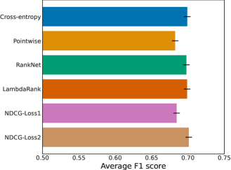
In the training data, we also have access to the raw scores for all candidate method on every dataset. Thus, instead of using a cross-entropy loss, it is also possible to treat the prediction problem as a learning-to-rank problem and apply rank-based loss functions (we refer the reader to Wang et al. [2018] for an overview of rank-based loss functions). We compare the cross-entropy to various rank-based loss functions (see Fig. 7) but find no significant improvement for our task. We use the allrank [Pobrotyn et al., 2020] and test the following rank-based losses: (i) Pointwise (where we directly regress the F1-scores for each candidate method), (ii) RankNet [Burges et al., 2005], (iii) LambdaRank [Burges, 2010], and (iv) NDCG-Loss1 and NDCG-Loss2 as described in Wang et al. [2018, Sec. 5.2].

Appendix C Additional results on the semi-synthetic and real-world benchmarks

For the four semi-synthetic and real-world benchmarks (see Sec. 5.3), we compute the F1-score for each candidate method by averaging the scores over $10$ runs (see Fig. 8 for the scores of each method on the four benchmarks). Next, we also show the predicted rankings of the six methods from CAMP-SemiSup and CAMP-Sup for each of the four benchmarks (see Table 3).

(a) MAGIC-NIAB

(b) MAGIC-IRRI

(c) SynTReN

(d) Protein cells

Figure 8: The F1 scores of the six causal discovery methods (averaged over $10$ runs of each method) on the four semi-synthetic and real-world benchmarks (for MAGIC-NIAB, the bar for DECI is missing because it outputs a nearly empty graph resulting in a zero F1 score).

Benchmarks	Predicted ranking (from best to worst)
MAGIC-NIAB
Oracle	DAG-GNN, NOTEARS-MLP, DirectLiNGAM, NOTEARS-linear, GranDAG, DECI
CAMP-SemiSup	DAG-GNN, NOTEARS-linear, NOTEARS-MLP, DECI, DirectLiNGAM, GranDAG
CAMP-Sup	DECI, NOTEARS-MLP, GranDAG, DAG-GNN, NOTEARS-linear, DirectLiNGAM
MAGIC-IRRI
Oracle	NOTEARS-linear, DirectLiNGAM, DAG-GNN, NOTEARS-MLP, GranDAG, DECI
CAMP-SemiSup	DAG-GNN, NOTEARS-linear, NOTEARS-MLP, DECI, DirectLiNGAM, GranDAG
CAMP-Sup	DECI, NOTEARS-MLP, DAG-GNN, GranDAG, NOTEARS-linear, DirectLiNGAM
SynTReN
Oracle	DAG-GNN, NOTEARS-linear, DECI, NOTEARS-MLP, GranDAG, DirectLiNGAM
CAMP-SemiSup	DAG-GNN, NOTEARS-linear, NOTEARS-MLP, DirectLiNGAM, GranDAG, DECI
CAMP-Sup	DAG-GNN, NOTEARS-linear, NOTEARS-MLP, DirectLiNGAM, DECI, GranDAG
Protein cells
Oracle	DirectLiNGAM, NOTEARS-linear, GranDAG, DECI, DAG-GNN, NOTEARS-MLP
CAMP-SemiSup	DirectLiNGAM, NOTEARS-linear, DAG-GNN, NOTEARS-MLP, GranDAG, DECI
CAMP-Sup	DirectLiNGAM, DAG-GNN, NOTEARS-linear, NOTEARS-MLP, DECI, GranDAG

Table 3: The predicted rankings of the six causal discovery methods from CAMP-SemiSup and CAMP-Sup for the four semi-synthetic and real-world benchmarks (also see Fig. 8 for the F1-scores of the various methods on each benchmark).

References

- Alaa and Van Der Schaar [2019] A. Alaa and M. Van Der Schaar. Validating causal inference models via influence functions. In International Conference on Machine Learning, 2019.
- Arlot and Celisse [2010] S. Arlot and A. Celisse. A survey of cross-validation procedures for model selection. Statistics Surveys, 2010. doi: 10.1214/09-SS054.
- Ashman et al. [2023] M. Ashman, C. Ma, A. Hilmkil, J. Jennings, and C. Zhang. Causal reasoning in the presence of latent confounders via neural ADMG learning. In International Conference on Learning Representations, 2023.
- Barabási and Albert [1999] A.-L. Barabási and R. Albert. Emergence of scaling in random networks. Science, 1999.
- Berrevoets et al. [2023] J. Berrevoets, K. Kacprzyk, Z. Qian, and M. van der Schaar. Causal deep learning. arXiv preprint arXiv:2303.02186, 2023.
- Biza et al. [2020] K. Biza, I. Tsamardinos, and S. Triantafillou. Tuning causal discovery algorithms. In International Conference on Probabilistic Graphical Models, 2020.
- Biza et al. [2022] K. Biza, I. Tsamardinos, and S. Triantafillou. Out-of-sample tuning for causal discovery. IEEE Transactions on Neural Networks and Learning Systems, 2022.
- Bommasani et al. [2021] R. Bommasani, D. A. Hudson, E. Adeli, R. Altman, S. Arora, S. von Arx, M. S. Bernstein, J. Bohg, A. Bosselut, E. Brunskill, et al. On the opportunities and risks of foundation models. arXiv preprint arXiv:2108.07258, 2021.
- Bubeck et al. [2023] S. Bubeck, V. Chandrasekaran, R. Eldan, J. Gehrke, E. Horvitz, E. Kamar, P. Lee, Y. T. Lee, Y. Li, S. Lundberg, et al. Sparks of artificial general intelligence: Early experiments with gpt-4. arXiv preprint arXiv:2303.12712, 2023.
- Burges et al. [2005] C. Burges, T. Shaked, E. Renshaw, A. Lazier, M. Deeds, N. Hamilton, and G. Hullender. Learning to rank using gradient descent. In International Conference on Machine learning, 2005.
- Burges [2010] C. J. Burges. From ranknet to lambdarank to lambdamart: An overview. Learning, 2010.
- Chase [2022] H. Chase. LangChain, Oct. 2022. URL https://github.com/langchain-ai/langchain.
- Chen et al. [2020] T. Chen, S. Kornblith, K. Swersky, M. Norouzi, and G. E. Hinton. Big self-supervised models are strong semi-supervised learners. Advances in neural information processing systems, 2020.
- Curth and van der Schaar [2023] A. Curth and M. van der Schaar. In search of insights, not magic bullets: Towards demystification of the model selection dilemma in heterogeneous treatment effect estimation. arXiv preprint arXiv:2302.02923, 2023.
- Dallas et al. [2017] S. Dallas, K. Machairas, and E. Papadopoulos. A comparison of ordinary differential equation solvers for dynamical systems with impacts. Journal of Computational and Nonlinear Dynamics, 2017.
- Faller et al. [2023] P. M. Faller, L. C. Vankadara, A. A. Mastakouri, F. Locatello, and D. Janzing. Self-compatibility: Evaluating causal discovery without ground truth. arXiv preprint arXiv:2307.09552, 2023.
- Geffner et al. [2022] T. Geffner, J. Antoran, A. Foster, W. Gong, C. Ma, E. Kiciman, A. Sharma, A. Lamb, M. Kukla, N. Pawlowski, M. Allamanis, and C. Zhang. Deep end-to-end causal inference. arXiv preprint arXiv:2202.02195, 2022.
- Gutierrez and Gérardy [2017] P. Gutierrez and J.-Y. Gérardy. Causal inference and uplift modelling: A review of the literature. In International Conference on Predictive Applications and APIs. PMLR, 2017.
- He et al. [2021] X. He, K. Zhao, and X. Chu. Automl: A survey of the state-of-the-art. Knowledge-Based Systems, 2021.
- Hutter et al. [2019] F. Hutter, L. Kotthoff, and J. Vanschoren. Automated machine learning: methods, systems, challenges. Springer Nature, 2019.
- Immer et al. [2023] A. Immer, C. Schultheiss, J. E. Vogt, B. Schölkopf, P. Bühlmann, and A. Marx. On the identifiability and estimation of causal location-scale noise models. In International Conference on Machine Learning, 2023.
- Ke et al. [2022] N. R. Ke, S. Chiappa, J. Wang, A. Goyal, J. Bornschein, M. Rey, T. Weber, M. Botvinic, M. Mozer, and D. J. Rezende. Learning to induce causal structure. arXiv preprint arXiv:2204.04875, 2022.
- Ke et al. [2023] N. R. Ke, S.-J. Dunn, J. Bornschein, S. Chiappa, M. Rey, J.-B. Lespiau, A. Cassirer, J. Wang, T. Weber, D. Barrett, et al. Discogen: Learning to discover gene regulatory networks. arXiv preprint arXiv:2304.05823, 2023.
- Keropyan et al. [2023] G. Keropyan, D. Strieder, and M. Drton. Rank-based causal discovery for post-nonlinear models. In International Conference on Artificial Intelligence and Statistics, 2023.
- Kiciman et al. [2022] E. Kiciman, E. W. Dillon, D. Edge, A. Foster, A. Hilmkil, J. Jennings, C. Ma, R. Ness, N. Pawlowski, A. Sharma, et al. A causal ai suite for decision-making. In NeurIPS 2022 Workshop on Causality for Real-world Impact, 2022.
- Kıcıman et al. [2023] E. Kıcıman, R. Ness, A. Sharma, and C. Tan. Causal reasoning and large language models: Opening a new frontier for causality. arXiv preprint arXiv:2305.00050, 2023.
- Kong et al. [2023] L. Kong, B. Huang, F. Xie, E. Xing, Y. Chi, and K. Zhang. Identification of nonlinear latent hierarchical models. arXiv preprint arXiv:2306.07916, 2023.
- Lachapelle et al. [2019] S. Lachapelle, P. Brouillard, T. Deleu, and S. Lacoste-Julien. Gradient-based neural dag learning. arXiv preprint arXiv:1906.02226, 2019.
- Li et al. [2020] H. Li, Q. Xiao, and J. Tian. Supervised whole dag causal discovery. arXiv preprint arXiv:2006.04697, 2020.
- Liu et al. [2010] H. Liu, K. Roeder, and L. Wasserman. Stability approach to regularization selection (stars) for high dimensional graphical models. Advances in neural information processing systems, 2010.
- Long et al. [2023] S. Long, A. Piché, V. Zantedeschi, T. Schuster, and A. Drouin. Causal discovery with language models as imperfect experts. arXiv preprint arXiv:2307.02390, 2023.
- Lorch et al. [2022] L. Lorch, S. Sussex, J. Rothfuss, A. Krause, and B. Schölkopf. Amortized inference for causal structure learning. Advances in Neural Information Processing Systems, 2022.
- Maathuis et al. [2009] M. H. Maathuis, M. Kalisch, and P. Bühlmann. Estimating high-dimensional intervention effects from observational data. The Annals of Statistics, 2009. doi: 10.1214/09-AOS685.
- Machlanski et al. [2023] D. Machlanski, S. Samothrakis, and P. Clarke. Hyperparameter tuning and model evaluation in causal effect estimation. arXiv preprint arXiv:2303.01412, 2023.
- Mahajan et al. [2022] D. Mahajan, I. Mitliagkas, B. Neal, and V. Syrgkanis. Empirical analysis of model selection for heterogenous causal effect estimation. arXiv preprint arXiv:2211.01939, 2022.
- Matthieu and Gaël [2023] D. Matthieu and V. Gaël. How to select predictive models for causal inference? arXiv preprint arXiv:2302.00370, 2023.
- Mohd Razali and Yap [2011] N. Mohd Razali and B. Yap. Power comparisons of shapiro-wilk, kolmogorov-smirnov, lilliefors and anderson-darling tests. J. Stat. Model. Analytics, 2, 01 2011.
- Ouyang et al. [2022] L. Ouyang, J. Wu, X. Jiang, D. Almeida, C. Wainwright, P. Mishkin, C. Zhang, S. Agarwal, K. Slama, A. Ray, et al. Training language models to follow instructions with human feedback. Advances in Neural Information Processing Systems, 35:27730–27744, 2022.
- Peters et al. [2014] J. Peters, J. M. Mooij, D. Janzing, and B. Schölkopf. Causal discovery with continuous additive noise models. Journal of Machine Learning Research, 2014.
- Peters et al. [2017] J. Peters, D. Janzing, and B. Schölkopf. Elements of causal inference: foundations and learning algorithms. The MIT Press, 2017.
- Petersen et al. [2022] A. H. Petersen, J. Ramsey, C. T. Ekstrøm, and P. Spirtes. Causal discovery for observational sciences using supervised machine learning. arXiv preprint arXiv:2202.12813, 2022.
- Pobrotyn et al. [2020] P. Pobrotyn, T. Bartczak, M. Synowiec, R. Bialobrzeski, and J. Bojar. Context-aware learning to rank with self-attention. arXiv, abs/2005.10084, 2020.
- Postawa et al. [2020] K. Postawa, J. Szczygieł, and M. Kułażyński. A comprehensive comparison of ode solvers for biochemical problems. Renewable Energy, 2020.
- Raghu et al. [2018] V. K. Raghu, A. Poon, and P. V. Benos. Evaluation of causal structure learning methods on mixed data types. In ACM SIGKDD Workshop on Causal Discovery, 2018.
- Raschka [2018] S. Raschka. Model evaluation, model selection, and algorithm selection in machine learning. arXiv preprint arXiv:1811.12808, 2018.
- Rolling and Yang [2014] C. A. Rolling and Y. Yang. Model selection for estimating treatment effects. Journal of the Royal Statistical Society Series B: Statistical Methodology, 2014.
- Sachs et al. [2005] K. Sachs, O. Perez, D. Pe’er, D. A. Lauffenburger, and G. P. Nolan. Causal protein-signaling networks derived from multiparameter single-cell data. Science, 2005.
- Saito and Yasui [2020] Y. Saito and S. Yasui. Counterfactual cross-validation: Stable model selection procedure for causal inference models. In International Conference on Machine Learning, 2020.
- Schick et al. [2023] T. Schick, J. Dwivedi-Yu, R. Dessì, R. Raileanu, M. Lomeli, L. Zettlemoyer, N. Cancedda, and T. Scialom. Toolformer: Language models can teach themselves to use tools. arXiv preprint arXiv:2302.04761, 2023.
- Schuler et al. [2018] A. Schuler, M. Baiocchi, R. Tibshirani, and N. Shah. A comparison of methods for model selection when estimating individual treatment effects. arXiv preprint arXiv:1804.05146, 2018.
- Scutari [2010] M. Scutari. Learning bayesian networks with the bnlearn R package. Journal of Statistical Software, 2010. doi: 10.18637/jss.v035.i03.
- Scutari et al. [2014] M. Scutari, P. Howell, D. J. Balding, and I. Mackay. Multiple quantitative trait analysis using bayesian networks. Genetics, 2014.
- Shimizu et al. [2011] S. Shimizu, T. Inazumi, Y. Sogawa, A. Hyvarinen, Y. Kawahara, T. Washio, P. O. Hoyer, K. Bollen, and P. Hoyer. Directlingam: A direct method for learning a linear non-gaussian structural equation model. Journal of Machine Learning Research (JMLR), 2011.
- Squires and Uhler [2022] C. Squires and C. Uhler. Causal structure learning: a combinatorial perspective. arXiv preprint arXiv:2206.01152, 2022.
- Strobl [2021] E. V. Strobl. Automated hyperparameter selection for the pc algorithm. Pattern Recognition Letters, 2021.
- Uemura et al. [2022] K. Uemura, T. Takagi, K. Takayuki, H. Yoshida, and S. Shimizu. A multivariate causal discovery based on post-nonlinear model. In Conference on Causal Learning and Reasoning, 2022.
- Van den Bulcke et al. [2006] T. Van den Bulcke, K. Van Leemput, B. Naudts, P. van Remortel, H. Ma, A. Verschoren, B. De Moor, and K. Marchal. Syntren: a generator of synthetic gene expression data for design and analysis of structure learning algorithms. BMC bioinformatics, 2006.
- Wang and Kording [2022] X. Wang and K. Kording. Meta-learning causal discovery. arXiv preprint arXiv:2209.05598, 2022.
- Wang et al. [2018] X. Wang, C. Li, N. Golbandi, M. Bendersky, and M. Najork. The lambdaloss framework for ranking metric optimization. In Proceedings of the 27th ACM international conference on information and knowledge management, pages 1313–1322, 2018.
- Wei et al. [2022] J. Wei, Y. Tay, R. Bommasani, C. Raffel, B. Zoph, S. Borgeaud, D. Yogatama, M. Bosma, D. Zhou, D. Metzler, E. H. Chi, T. Hashimoto, O. Vinyals, P. Liang, J. Dean, and W. Fedus. Emergent abilities of large language models. Transactions on Machine Learning Research, 2022.
- Yao et al. [2021] L. Yao, Z. Chu, S. Li, Y. Li, J. Gao, and A. Zhang. A survey on causal inference. ACM Transactions on Knowledge Discovery from Data (TKDD), 2021.
- Yu et al. [2019] Y. Yu, J. Chen, T. Gao, and M. Yu. Dag-gnn: Dag structure learning with graph neural networks. International Conference on Machine Learning, 2019.
- Zevcević et al. [2023] M. Zevcević, M. Willig, D. S. Dhami, and K. Kersting. Causal parrots: Large language models may talk causality but are not causal. Transactions on Machine Learning Research, 2023.
- Zhai et al. [2019] X. Zhai, A. Oliver, A. Kolesnikov, and L. Beyer. S4l: Self-supervised semi-supervised learning. In Proceedings of the IEEE/CVF international conference on computer vision, 2019.
- Zhang et al. [2023] C. Zhang, S. Bauer, P. Bennett, J. Gao, W. Gong, A. Hilmkil, J. Jennings, C. Ma, T. Minka, N. Pawlowski, et al. Understanding causality with large language models: Feasibility and opportunities. arXiv preprint arXiv:2304.05524, 2023.
- Zhang and Hyvarinen [2012] K. Zhang and A. Hyvarinen. On the identifiability of the post-nonlinear causal model. arXiv preprint arXiv:1205.2599, 2012.
- Zhang et al. [2021] K. Zhang, S. Zhu, M. Kalander, I. Ng, J. Ye, Z. Chen, and L. Pan. gcastle: A python toolbox for causal discovery. arXiv preprint arXiv:2111.15155, 2021.
- Zheng et al. [2018] X. Zheng, B. Aragam, P. K. Ravikumar, and E. P. Xing. Dags with no tears: Continuous optimization for structure learning. Advances in neural information processing systems, 2018.
- Zheng et al. [2020] X. Zheng, C. Dan, B. Aragam, P. Ravikumar, and E. Xing. Learning sparse nonparametric dags. International Conference on Artificial Intelligence and Statistics, 2020.