Computation of the Distribution of the Absorption Time of the Drifted Diffusion with Stochastic Resetting and Mixed Boundary Conditions

Abstract

This article introduces two techniques for computing the distribution of the first passage or absorption time of a drifted Wiener diffusion with Poisson resetting times, in presence of an upper hard wall reflection and a lower absorbing barrier. The first method starts with the Padé approximation to the Laplace transform of the first passage time, which is then inverted through the partial fraction decomposition. The second method, which we call “multiresolution algorithm”, is a Monte Carlo technique that exploits the properties of the Wiener process in order to generate Brownian bridges at increasing resolution levels. This technique allows to approximate the first passage time at any level of accuracy. An intensive numerical study reveals that the multiresolution algorithm has higher accuracy than standard Monte Carlo, whereas the faster method based on the Padé approximation provides sufficient accuracy in specific circumstances only. Besides these two numerical approximations, this article provides a closed-form expression for the expected first passage time.

[1]organization=Institute of Mathematical Statistics and Actuarial Science, University of Bern,addressline=Alpeneggstrasse 22, city=Bern, postcode=3012, country=Switzerland

[2]organization=Department of Visceral Surgery and Medicine, Inselspital, Bern University Hospital, University of Bern,addressline=Murtenstrasse 35, city=Bern, postcode=3008, country=Switzerland

[3]organization=Group Risk Management, Swiss Re Management Ltd,addressline=Mythenquai 50/60, city=Zurich, postcode=8022, country=Switzerland

[4]organization=Instituto de Fisica Interdisciplinar y Sistemas Complejos IFISC (CSIC-UIB),addressline=Campus UIB, city=Palma de Mallorca, postcode=07122, country=Spain

1 Introduction

Drift-diffusion processes are a key part of mathematical models in multiple disciplines, from physics [1, 2, 3, 4] to mathematical finance [5, 6]. They are also frequently used in biology, some examples being prey-predator dynamics [7] and coordinated cellular migration [8]. Mathematically, these processes are governed by stochastic differential equations (SDE) [9, 10] and referred to as Brownian motion. First passage times (FPT) are the typical quantities of interest in such models and their probability distribution, when available, provides essential information for scientific investigations [11]. In most cases of interest, this distribution cannot be obtained analytically and one must rely on numerical techniques. This article introduces two novel computational methods for obtaining the distribution of the FPT of a drifted Brownian motion with Poisson resetting times, in the presence of an upper hard wall reflection and a lower absorbing barrier. The two techniques complement themselves in the sense that the first one, based on the Padé approximation, is fast to compute but has limited accuracy, whereas the other one, based on Monte Carlo, is computationally intensive but also very accurate.

Drift-diffusion processes have been studied in multiple spaces, such as bounded regions and arbitrary dimensions [11, 12, 13, 14]. Of particular interest are problems with absorbing or reflecting boundaries. Absorbing boundaries are regions in the diffusion space where diffusing particles can enter but cannot leave. Reflecting boundaries are regions in which diffusing particles cannot permeate [15]. The theory of stochastic processes with absorbing and reflecting boundaries is a classical topic in probability theory, see for example [16]. Regarding its application, these boundaries have been considered for modelling DNA searching of proteins using partially-reflecting obstacles [17] and prey-predator dynamics in a finite lattice [18].

First passage problems have been used in various fields such as solid state physics [19], cosmology [20], economics [21], and finance [22]. In mathematical biology, FPTs have been used to study how fast two DNA segments in the genome have physical contact [23], epidemiology [24], and cellular channel transport and receptor binding [25].

Among first passage problems, stochastic resetting problems have gained importance in the past decade [26, 27, 28]. Stochastic resetting occurs when the particle returns to its initial position at random times. Solutions to the Fokker-Planck equation with resetting have been investigated, especially for systems with absorbing boundaries [29, 30, 31]. Resetting has also been generalized to power-law distributed resetting [32], time-dependent resetting [33], as well as with Lévy flights [34] and Ornstein-Uhlenbeck processes [35].

Within the context of statistical physics, processes involving stochastic resetting serve as a paradigm for intrinsically out-of-equilibrium systems, as they exhibit nonequilibrium stationary distributions [29]. Furthermore, in the context of biology, stochastic resetting has been used to model hunting behavior in animals, where animals return to specific sites to look for food [36]. At the cellular level, this scheme has also been used to model cellular focal adhesions [37]. At biomolecular level, this has been used to model backtrack recovery in RNA polymerization [38]. As new models and experimental realizations of processes with stochastic resetting continue to emerge [39, 40], there is a growing need for more refined theories and simulations to comprehensively characterize real-world resetting protocols [29], which we tackle to some extent in this study.

In our previous work, we have shown that a drift-diffusion process with mixed boundary conditions and stochastic resetting can be used to model drug resistance development [41]. Drug resistance development is a consequence of mutation, which is a noisy process that is biased towards survival of the infecting pathogen [42, 43]. From this, we used a drift-diffusion process on a bounded interval with resetting to quantify the change in therapy efficacy of a mutating infecting pathogen.

On the interval, the reflecting boundary represents a perfect therapy and the absorbing boundary represents drug failure or patient death. Eventually, the infecting pathogens develop complete resistances to therapies due to mutation [44]. As such, we defined the FPT as the time when the stochastic process reaches the absorbing boundary.

Stochastic resetting represents changing the therapy being administered to a patient, which is a common strategy used by physicians to avoid the development of drug resistance [45]. Changing the therapy exposes the pathogen to a new stimulus, which resets its resistance back to its initial value. This also means that the stochastic process resets to its initial position under stochastic resetting.

In [41], we were able to find the mean resistance development time for the aforementioned drug resistance model with therapy changes. However, the mean FPT is insufficient for a comprehensive understanding of the entire process. This is because important quantities such as the uncertainty, median, and quantiles are not available. Indeed, having knowledge of the entire FPT distribution gives a robust description of the model and has potential applications to biology and medicine. Presently, only the expression for the Laplace-transformed distribution of the FPT is known [41]. This is due to the absence of a straightforward method to obtain an inversion of the Laplace transform [46, 47]. To tackle the problem, we will introduce approximations to the inversion, alongside improved numerical simulations to obtain the distribution of the FPT [48, 49].

This article has the following structure. We start by presenting a compact re-expression of the mean FPT (Section 2) and we then introduce an approach based on the Padé approximation for obtaining the Laplace inversion of the FPT (Section 3). In order to obtain higher accuracy, we propose an alternative Monte Carlo approach, the multiresolution algorithm, that allows to control the error at any desired level. The implementation taking into account the special characteristics of our stochastic resetting model are presented in detail (Section 4). A short summary of the methodological and numerical results and a discussion on future research conclude the article (Section 5).

2 Mean absorption time

The distribution of FPTs is often the essential element in the study of first passage phenomena. It is however not immediately available since it involves solving a bounded Fokker-Planck equation at the absorbing boundary, which is not a straightforward task [11, 13, 14]. Nonetheless, we are still able to characterize the FPTs through Laplace transforms or moments.

In this section, we derive the Laplace transform of the FPT and obtain a novel formula for its expectation. Starting with the process without resetting, we obtain the Laplace-transformed propagator by solving the Laplace-transformed Fokker-Planck equation with boundary conditions [16] (Section 2.1). From the propagator, we obtain the Laplace-transformed FPT distribution [11, 41] that will relate to the process with resetting through the survival function [30, 31] (Section 2.2). Finally, by using the aforementioned expressions, we show that the expected FPT with resetting can be expressed in terms of the Laplace-transformed FPT distribution without resetting.

2.1 Derivation of the Laplace transformed propagator of the stochastic process without resetting

The initial model for the therapy efficacy is the Brownian motion or Wiener process with drift, denoted $X$, which solves the SDE

$$dX_{t}=v\,dt+\sqrt{2D}\,dW_{t},\quad t\geq 0\,,$$ (2.1)

with fixed initial condition $X_{0}=x_{0}\in(0,1]$, where the drift $v$ and the volatility $D$ are respectively real and nonnegative real constants. We then impose that the paths of the process $X$ are bounded between $0$ and $1$. On the one hand, the level 1 is a reflecting boundary of type hard wall, as described in Section 3.5 of [11]. The definition of this reflecting boundary requires the concept of probability current and will be given in equation (2.4). On the other hand, the level 0 is an absorbing state. Note that it is neither the reflection of a trajectory, as would be the absolute value of a diffusion, nor the regulated Brownian motion. These two cases are described in the introduction of [50].

Denote by $p(\cdot,t)$, for $t\geq 0$, the so-called propagator, that is the probability density of $X_{t}$, the forward Kolmogorov or Fokker-Planck equation is given by

$$\partial_{t}{p}(x,t)+vp^{\prime}(x,t)-Dp^{\prime\prime}(x,t)=0\,,$$ (2.2)

where, for a function $f(t,x)$, $\partial_{t}{f}$ denotes its partial derivative with respect to $t$ and $f^{\prime}$ (respectively $f^{\prime\prime}$) denotes the first (respectively second) partial derivative with respect to $x$, see e.g. [16].

Note that, throughout this section, we interpret the propagator as a defective probability distribution function, i.e. we forget about the probability mass corresponding to the absorption state. This reflects the physical interpretation of $X$ as the location of a particle moving between two boundaries that as soon as touches the absorbing boundary gets immediately removed from the system.

Let us further introduce the probability current

$$J(x,t)=vp(x,t)-Dp^{\prime}(x,t)\,.$$ (2.3)

Then, the boundary conditions may be defined in terms of the propagator and the probability current in the following way (see Chapter 4 of [9] and [11]):

$$p(0,t)=0\quad\text{and}\quad J(1,t)=0\,,\quad\forall\,t\geq 0\,.$$ (2.4)

Thus, we study the solution of the following system:

$$\left\{\begin{array}[]{ll}\partial_{t}{p}(x,t)+vp^{\prime}(x,t)-Dp^{\prime\prime}(x,t)=0,\\ p(0,t)=0\quad\text{and}\quad J(1,t)=0\,,\quad\forall\,t\geq 0\,,\\ p(x,0)=\delta(x-x_{0}),\end{array}\right.$$ (2.8)

where $\delta(x)$ is the Dirac delta function (that assigns mass 1 to $x=0$). Thus, the last equation in (2.8) provides the initial condition.

As far as the authors know, there is no closed analytical solution to the system (2.8). Therefore, we solve instead the equation obtained from the Laplace transform of $p(x,t)$.

The Laplace transform of any function $f(t)$ of the positive real line is hereafter denoted by adding a tilde on top of the function name,

$$\mathcal{L}(f)(s)=\tilde{f}(s)=\int_{0}^{\infty}e^{-st}f(t)\,dt\,,\quad s\geq 0\,.$$

In particular

$$\tilde{p}(x,s)=\int_{0}^{\infty}e^{-st}p(x,t)\,dt\,,\quad s\geq 0\,$$

and we obtain the following Lemma.

Lemma 2.1 (Laplace-transformed propagator).

We assume $x_{0}\in(0,1]$, $v\in\mathbb{R}$ and $D>0$ and we consider $p$ solution of (2.8). We define

$$\rho =\dfrac{v}{2D},\quad\omega(s)=\sqrt{v^{2}+4Ds},\quad\text{ and }\quad\theta(s)=\dfrac{\omega(s)}{2D}=\dfrac{\sqrt{v^{2}+4Ds}}{2D}.$$ (2.9)

Where the ratio $\rho$ is also called the Péclet number. By denoting, for $s>-v^{2}/(4D)$,

$$\alpha_{\pm}(s)=\frac{v\pm\sqrt{v^{2}+4Ds}}{2D}=\frac{v\pm\omega(s)}{2D}=\rho\pm\theta(s)\,,$$ (2.10)

we obtain the following expression for the Laplace transform of the propagator for all $s>-v^{2}/(4D)$,

$$\tilde{p}(x,s)=\tilde{p}(x_{0},s)\frac{e^{\alpha_{+}(s)x}-e^{\alpha_{-}(s)x}}{e^{\alpha_{+}(s)x_{0}}-e^{\alpha_{-}(s)x_{0}}}\,,\quad x\in[0,x_{0}),$$ (2.11)

and

$$\tilde{p}(x,s)=\tilde{p}(x_{0},s)\frac{\alpha_{+}(s)\,e^{\alpha_{+}(s)(x-1)}-\alpha_{-}(s)\,e^{\alpha_{-}(s)(x-1)}}{\alpha_{+}(s)\,e^{\alpha_{+}(s)(x_{0}-1)}-\alpha_{-}(s)\,e^{\alpha_{-}(s)(x_{0}-1)}}\,,\quad x\in(x_{0},1]\,,$$ (2.12)

with $\tilde{p}(x_{0},s)$ defined as

$$\tilde{p}(x_{0},s) =\frac{2\,\mathrm{sinh}(\theta x_{0})\left\{\omega\,\mathrm{cosh}[\theta(x_{0}-1)]+v\,\mathrm{sinh}[\theta(x_{0}-1)]\right\}}{\omega^{2}\,\mathrm{cosh}(\theta)-v\,\omega\,\mathrm{sinh}(\theta)}\,.$$ (2.13)

Proof.

First, note that swapping integral and derivative operation over different variables yields

$$\mathcal{L}\left(vp^{\prime}(x,\cdot)\right)(s)=v\tilde{p}^{\prime}(x,s)\,\quad\text{and}\quad\mathcal{L}\left(Dp^{\prime\prime}(x,\cdot)\right)(s)=D\tilde{p}^{\prime\prime}(x,s)\,.$$

Moreover, for $x\in[0,x_{0})\cup(x_{0},1]$, integration by parts formula provides

$$\int_{0}^{\infty}e^{-st}\partial_{t}{p}(x,t)\,dt=e^{-st}p(x,t)\Big{|}_{0}^{\infty}+s\int_{0}^{\infty}e^{-st}p(x,t)\,dt=s\tilde{p}(x,s).$$

(Note that we cannot exactly evaluate $p(x,t)$ at $t=0$, but for $x\neq x_{0}$ we can take the limit as $t\to 0$, which corresponds to applying integration by parts on compacts $[n^{-1},n]$ and then let $n\to\infty$.) Therefore, the transformed Kolmogorov equation (2.2) for $\tilde{p}(x,s)$ is given by

$$s\tilde{p}(x,s)+v\tilde{p}^{\prime}(x,s)-D\tilde{p}^{\prime\prime}(x,s)=0\,,\quad s\geq 0\,,$$ (2.14)

for $x\in[0,x_{0})\cup(x_{0},1]$.

In order to find a solution to (2.14), let us fix $s$, denote $\tilde{p}_{<}(x)=\tilde{p}(x,s)$ for $x\in[0,x_{0})$, $\tilde{p}_{>}(x)=\tilde{p}(x,s)$ for $x\in(x_{0},1]$ and search an analytic solution to

$$D\tilde{p}^{\prime\prime}(x)-v\tilde{p}^{\prime}(x)-s\tilde{p}(x)=0,$$

over these two intervals. The characteristic equation is

$$D\alpha^{2}-v\alpha-s=0\,,$$

with roots, defined in (2.10),

$$\alpha_{\pm}=\frac{v\pm\sqrt{v^{2}+4Ds}}{2D}=\frac{v\pm\omega(s)}{2D}=\rho\pm\theta(s)\,,$$

where the constants are defined by (2.9). Therefore,

$$\tilde{p}_{>}(x)=Ae^{\alpha_{+}x}+Be^{\alpha_{-}x}\quad\text{and}\quad\tilde{p}_{<}(x)=ae^{\alpha_{+}x}+be^{\alpha_{-}x}\,,$$

for some constants $a$, $b$, $A$ and $B$ to be determined. From the boundary conditions (2.4) we obtain

$$\tilde{p}_{<}(x)=a(e^{\alpha_{+}x}-e^{\alpha_{-}x})$$

and

$$v(Ae^{\alpha_{+}}+Be^{\alpha_{-}})=D(\alpha_{+}Ae^{\alpha_{+}}+\alpha_{-}Be^{\alpha_{-}})\,.$$

The latter equation may be rewritten as

$$(D\alpha_{+}-v)Ae^{\alpha_{+}}=(v-D\alpha_{-})Be^{\alpha_{-}}=C(s)\,,$$

implying

$$\tilde{p}_{>}(x)=C\left(\frac{e^{\alpha_{+}(x-1)}}{D\alpha_{+}-v}+\frac{e^{\alpha_{-}(x-1)}}{v-D\alpha_{-}}\right)\,.$$

The continuity of $p(\cdot,t)$ (see [10], Chapter 15, section 5) yields $\tilde{p}_{<}(x_{0})=\tilde{p}_{>}(x_{0})$, hence one can write

$$C\left(\frac{e^{\alpha_{+}(x_{0}-1)}}{D\alpha_{+}-v}+\frac{e^{\alpha_{-}(x_{0}-1)}}{v-D\alpha_{-}}\right)=a\left(e^{\alpha_{+}x_{0}}-e^{\alpha_{-}x_{0}}\right)=c(s).$$

Consequently, we obtain

$$\tilde{p}_{<}(x)=c(s)\frac{e^{\alpha_{+}x}-e^{\alpha_{-}x}}{e^{\alpha_{+}x_{0}}-e^{\alpha_{-}x_{0}}}\;\text{ and }\;\tilde{p}_{>}(x)=c(s)\frac{\frac{e^{\alpha_{+}(x-1)}}{D\alpha_{+}-v}+\frac{e^{\alpha_{-}(x-1)}}{v-D\alpha_{-}}}{\frac{e^{\alpha_{+}(x_{0}-1)}}{D\alpha_{+}-v}+\frac{e^{\alpha_{-}(x_{0}-1)}}{v-D\alpha_{-}}}\,.$$

Noticing

$$v-D\alpha_{-}=D\alpha_{+}\quad\text{and}\quad v-D\alpha_{+}=D\alpha_{-},$$

we have

$$\tilde{p}_{>}(x)=c(s)\frac{\alpha_{+}e^{\alpha_{+}(x-1)}-\alpha_{-}e^{\alpha_{-}(x-1)}}{\alpha_{+}e^{\alpha_{+}(x_{0}-1)}-\alpha_{-}e^{\alpha_{-}(x_{0}-1)}}\,.$$

Our goal is now to determine the function $c(s)=\tilde{p}(x_{0},s)$.

We proceed to examine conditions involving the derivative of $p$ following standard procedures (see e.g. p. 16 of [11] or p. 449 of [51]). Let us rewrite (2.14) for $x\in[0,1]$ by means of the Dirac delta $\delta(x-x_{0})$:

$$s\tilde{p}(x,s)+v\tilde{p}^{\prime}(x,s)-D\tilde{p}^{\prime\prime}(x,s)=\delta(x-x_{0})\,,\quad s\geq 0\,.$$

Integrating the above equation on a segment around $x_{0}$,

$$\int_{x_{0}-\epsilon}^{x_{0}+\epsilon}\left\{s\tilde{p}(x,s)+v\tilde{p}^{\prime}(x,s)-D\tilde{p}^{\prime\prime}(x,s)\right\}\,dx =\int_{x_{0}-\epsilon}^{x_{0}+\epsilon}\delta(x-x_{0})\,dx\,,\quad s\geq 0\,,\epsilon>0$$

then,

$$\int_{x_{0}-\epsilon}^{x_{0}+\epsilon}\left(s\tilde{p}(x,s)\right)\,dx+v\tilde{p}(x,s)\Big{|}_{x_{0}-\epsilon}^{x_{0}+\epsilon}\ -D\tilde{p}^{\prime}(x,s)\Big{|}_{x_{0}-\epsilon}^{x_{0}+\epsilon} =1.$$

In the limit $\epsilon\rightarrow 0$, the first two terms at the left-hand side tend to zero due to continuity of $\tilde{p}(x,s)$ at $x=x_{0}$. While the third summand can be evaluated in terms of $\tilde{p}^{\prime}_{<}$ and $\tilde{p}^{\prime}_{>}$,

$$D\left(\tilde{p}^{\prime}_{<}(x_{0})-\tilde{p}^{\prime}_{>}(x_{0})\right)=1\,.$$ (2.15)

Let us compute the first derivative

$$\tilde{p}^{\prime}_{<}(x)=c\frac{\alpha_{+}e^{\alpha_{+}x}-\alpha_{-}e^{\alpha_{-}x}}{e^{\alpha_{+}x_{0}}-e^{\alpha_{-}x_{0}}}\,,$$

and evaluate it at $x_{0}$

$$\tilde{p}^{\prime}_{<}(x_{0}) =c\frac{\alpha_{+}e^{\alpha_{+}x_{0}}-\alpha_{-}e^{\alpha_{-}x_{0}}}{e^{\alpha_{+}x_{0}}-e^{\alpha_{-}x_{0}}}$$

$$=c\frac{\alpha_{+}e^{\theta x_{0}}-\alpha_{-}e^{-\theta x_{0}}}{e^{\theta x_{0}}-e^{-\theta x_{0}}}\,.$$

Analogously,

$$\tilde{p}^{\prime}_{>}(x)=c\frac{\alpha_{+}^{2}e^{\alpha_{+}(x-1)}-\alpha_{-}^{2}e^{\alpha_{-}(x-1)}}{\alpha_{+}e^{\alpha_{+}(x_{0}-1)}-\alpha_{-}e^{\alpha_{-}(x_{0}-1)}}\,,$$

leads to

$$\tilde{p}^{\prime}_{>}(x_{0}) =c\frac{\alpha_{+}^{2}e^{\alpha_{+}(x_{0}-1)}-\alpha_{-}^{2}e^{\alpha_{-}(x_{0}-1)}}{\alpha_{+}e^{\alpha_{+}(x_{0}-1)}-\alpha_{-}e^{\alpha_{-}(x_{0}-1)}}$$

$$=c\frac{\alpha_{+}^{2}e^{\theta(x_{0}-1)}-\alpha_{-}^{2}e^{-\theta(x_{0}-1)}}{\alpha_{+}e^{\theta(x_{0}-1)}-\alpha_{-}e^{-\theta(x_{0}-1)}}\,.$$

Therefore, plugging (2.15)

$$1 =Dc\left(\frac{\alpha_{+}e^{\theta x_{0}}-\alpha_{-}e^{-\theta x_{0}}}{e^{\theta x_{0}}-e^{-\theta x_{0}}}-\frac{\alpha_{+}^{2}e^{\theta(x_{0}-1)}-\alpha_{-}^{2}e^{-\theta(x_{0}-1)}}{\alpha_{+}e^{\theta(x_{0}-1)}-\alpha_{-}e^{-\theta(x_{0}-1)}}\right)$$

$$=Dc\,\frac{e^{-\theta}(\alpha_{+}^{2}-\alpha_{+}\alpha_{-})+e^{\theta}(\alpha_{-}^{2}-\alpha_{+}\alpha_{-})}{\alpha_{+}e^{\theta(2x_{0}-1)}+\alpha_{-}e^{-\theta(2x_{0}-1)}-\alpha_{+}e^{-\theta}-\alpha_{-}e^{\theta}}$$

$$=2Dc\,\frac{e^{-\theta}\theta(\theta+\rho)+e^{\theta}\theta(\theta-\rho)}{\alpha_{+}e^{\theta(2x_{0}-1)}+\alpha_{-}e^{-\theta(2x_{0}-1)}-\alpha_{+}e^{-\theta}-\alpha_{-}e^{\theta}}$$

$$=2Dc\,\frac{\theta(\theta\,\mathrm{cosh}(\theta)-\rho\,\mathrm{sinh}(\theta))}{\rho\,\mathrm{cosh}[\theta(2x_{0}-1)]+\theta\,\mathrm{sinh}[\theta(2x_{0}-1)]-\rho\,\mathrm{cosh}(\theta)+\theta\,\mathrm{sinh}(\theta)}$$

$$=c\,\frac{\omega(\omega\,\mathrm{cosh}(\theta)-v\,\mathrm{sinh}(\theta))}{v\,\mathrm{cosh}[\theta(2x_{0}-1)]+\omega\,\mathrm{sinh}[\theta(2x_{0}-1)]-v\,\mathrm{cosh}(\theta)+\omega\,\mathrm{sinh}(\theta)}\,,$$

which gives

$$c(s)=\tilde{p}(x_{0},s) =\frac{v\,\mathrm{cosh}[\theta(2x_{0}-1)]+\omega\,\mathrm{sinh}[\theta(2x_{0}-1)]-v\,\mathrm{cosh}(\theta)+\omega\,\mathrm{sinh}(\theta)}{\omega^{2}\,\mathrm{cosh}(\theta)-v\omega\,\mathrm{sinh}(\theta)}$$

$$=\frac{2\,\mathrm{sinh}(\theta x_{0})\left\{\omega\,\mathrm{cosh}[\theta(x_{0}-1)]+v\,\mathrm{sinh}[\theta(x_{0}-1)]\right\}}{\omega^{2}\,\mathrm{cosh}(\theta)-v\,\omega\mathrm{sinh}(\theta)}\,,$$

where $\omega$ and $\theta$ are defined in (2.9). All in all, we obtain the expressions (2.11), (2.12) and (2.13) for the Laplace transform of the propagator. ∎

2.2 Derivation of the Laplace-transformed propagator of the process with resetting

We now modify the dynamics of the above-defined stochastic process by incorporating a stochastic resetting effect. More explicitly, we assume that at homogeneous Poisson times $0<T_{1}<T_{2}<\ldots$, a.s., the value of the process $X$ is reset to its initial value $x_{0}$. Following [29], this is expressed through the inclusion of an additional term to the SDE that accounts for the magnitude of the jumps as follows,

$$dX_{t}=(1-\chi_{t})\cdot(v\,dt+\sqrt{2D}\,dW_{t})+\chi_{t}\cdot(x_{0}-X_{t}),\quad t\geq 0\,,$$ (2.16)

where the newly appearing stochastic process $\chi$ is an independent homogeneous Poisson process with rate or intensity $r>0$. Namely,

$$\chi_{t}=\sum_{n=1}^{\infty}\mathbf{1}\{T_{n}=t\},\quad t\geq 0,$$

where $\mathbf{1}$ denotes the indicator and $T_{n}$ is the sum of $n$ independent exponential random variables with expectation $r^{-1}$, representing the inter-occurrence times, for any positive integer $n$.

The FPT of interest, also called absorption time, is given by

$$\tau_{r}=\inf\{t\geq 0\,|\,X_{t}=0\},$$ (2.17)

which admits a probability density function $f_{r}$. Here, the subscript $r$ highlights the dependency on the Poisson resetting rate $r$. When $r=0$, we obtain the dynamic without jumps. We now obtain a closed-form expression for the mean absorption time with resetting.

Proposition 2.2 (Mean absorption time).

When the process $X$ is solution of the SDE with resetting (2.16), with $X_{0}=x_{0}\in(0,1]$, $v\in\mathbb{R}$, $D>0$ and $r>0$, the expectation of $\tau_{r}$ in (2.17) is given by

$$\mathbb{E}\tau_{r}=\frac{1}{r}\left\{\frac{e^{\rho x_{0}}\,(\omega(r)\,\mathrm{cosh}\{\theta(r)\}-v\,\mathrm{sinh}\{\theta(r)\})}{\omega(r)\,\mathrm{cosh}\{\theta(r)(x_{0}-1)\}+v\,\mathrm{sinh}\{\theta(r)(x_{0}-1)\}}-1\right\},$$ (2.18)

where $\rho$, $\omega$ and $\theta$ are defined in (2.9).

Proof.

Let us define the distribution function of $\tau_{r}$ by $F_{r}(t)=\int_{0}^{t}f_{r}(s)ds$ and its survival function by $S_{r}(t)=1-F_{r}(t)=\mathbb{P}(\tau_{r}>t)$, $t\geq 0$. In view of the known relation

$$f_{r}(t)=-\partial_{t}{S}_{r}(t)\,,$$ (2.19)

we may re-express the expectation of interest in the following way:

$$\mathbb{E}\tau_{r}=\int_{0}^{\infty}tf_{r}(t)\,dt=-\int_{0}^{\infty}t\partial_{t}{S}_{r}(t)\,dt=\int_{0}^{\infty}S_{r}(t)\,dt=\tilde{S}_{r}(0)\,,$$ (2.20)

where the tilde always denotes the Laplace transform of a function. In order to find an expression for the latter term, we use a renewal equation that connects the survival function in the resetting case to the survival function for the evolution without resetting. The following equation is well-known in the literature relative to stochastic resetting and can be found e.g. in [29, 30, 31]

$$S_{r}(t)=e^{-rt}S_{0}(t)+r\int_{0}^{t}e^{-ru}S_{0}(u)S_{r}(t-u)\,du\,.$$

By taking Laplace transform on both sides yields

$$\tilde{S}_{r}(s)=\tilde{S}_{0}(s+r)+r\tilde{S}_{0}(s+r)\tilde{S}_{r}(s)\,,$$

hence, for all $s$ such that $\tilde{S}_{0}(s+r)\neq r^{-1}$,

$$\tilde{S}_{r}(s)=\frac{\tilde{S}_{0}(s+r)}{1-r\tilde{S}_{0}(s+r)}\,.$$ (2.21)

The link between $\tilde{S}_{0}(s)$ and $\tilde{f}_{0}(s)$ is provided by Laplace transforming (2.19) for $r=0$ that yields, for all $s\neq 0$,

$$\tilde{S}_{0}(s)=\frac{1-\tilde{f}_{0}(s)}{s}\,.$$

Plugging the latter into (2.21) gives for all $s\neq-r$ such that $\tilde{f}_{0}(s+r)\neq-s/r$,

$$\tilde{S}_{r}(s)=\frac{1-\tilde{f}_{0}(s+r)}{s+r\tilde{f}_{0}(s+r)}\,,$$ (2.22)

and by (2.20) we finally obtain

$$\mathbb{E}\tau_{r}=\frac{1}{r}\left\{\frac{1}{\tilde{f}_{0}(r)}-1\right\}\,.$$ (2.23)

All that remains to do is expressing $\tilde{f}$ in terms of what we explicitly know, that is $\tilde{p}$. This is done by considering the known relation

$$\tilde{f}_{0}(s)=D\tilde{p}^{\prime}(0,s)-v\tilde{p}(0,s)=D\tilde{p}^{\prime}(0,s)$$ (2.24)

which may be found e.g. in [11, 41]. Therefore, from Equation (2.24) we obtain for
$s>-v^{2}/(4D)$

$$\tilde{f}_{0}(s)=e^{-\rho x_{0}}\frac{\omega(s)\,\mathrm{cosh}\{\theta(s)(x_{0}-1)\}+v\,\mathrm{sinh}\{\theta(s)(x_{0}-1)\}}{\omega(s)\,\mathrm{cosh}\{\theta(s)\}-v\,\mathrm{sinh}\{\theta(s)\}}\,,$$ (2.25)

as it has been previously shown in [52] and plugging the latter into (2.23) yields an explicit analytic expression for the mean absorption time

$$\mathbb{E}\tau_{r}=\frac{1}{r}\left\{\frac{e^{\rho x_{0}}\,(\omega(r)\,\mathrm{cosh}\{\theta(r)\}-v\,\mathrm{sinh}\{\theta(r)\})}{\omega(r)\,\mathrm{cosh}\{\theta(r)(x_{0}-1)\}+v\,\mathrm{sinh}\{\theta(r)(x_{0}-1)\}}-1\right\}\,,$$

where $\rho$, $\omega$ and $\theta$ have been defined in (2.9). ∎

3 Inversion of Laplace transform by Padé approximation

The expected value of the absorption time or FPT $\tau_{r}$, defined in (2.17), does not always quantify sufficiently well the uncertainty inherent to the first passage phenomenon. Often, high-order quantiles are more relevant. Thus, one may want to obtain the entire probability distribution of $\tau_{r}$. Although its Laplace inverse is available, there is no obvious way of inverting it. The well-known fast Fourier transform (FFT) does not necessarily provide accurate results, in particular with high-order quantiles. We refer for example to [6] for a numerical comparison of methods for computing a FPT probability for the compound Poisson process perturbed by diffusion.

In this section, we propose and implement a particular method for our FPT problem. We obtain the Laplace-transformed FPT law (Section 3.1), whose inversion will be approximated numerically. The approximated inversion begins with the Padé approximation of the Laplace transform, followed by a partial fraction decomposition of the Padé approximant and by the obvious inversion of the sum of partial fractions (Section 3.2). One can find several references in the engineering literature on the problem of obtaining approximate Laplace inversions by rational approximations. Some early references are [46], [47], [48], [53] and [54].

3.1 Laplace transform of the law of the FPT for the model with resetting

Proposition 3.1 (Laplace transform of FPT with resetting).

Assume that $X$ is a solution of the SDE (2.16), with $X_{0}=x_{0}\in(0,1]$, $v\in\mathbb{R}$, $D>0$ and $r>0$. Denote by $f_{r}$ the probability density of the absorption time $\tau_{r}$ defined in (2.17). Then its Laplace transform is given by

$$\tilde{f}_{r}(s) =\frac{(s+r)\tilde{f}_{0}(s+r)}{s+r\tilde{f}_{0}(s+r)}$$

$${\textstyle=\frac{(s+r)\left\{\omega(s+r)\,\mathrm{cosh}[\theta(s+r)(x_{0}-1)]+v\,\mathrm{sinh}[\theta(s+r)(x_{0}-1)]\right\}}{se^{\rho x_{0}}\left\{\omega(s+r)\,\mathrm{cosh}[\theta(s+r)]-v\,\mathrm{sinh}[\theta(s+r)]\right\}+r\left\{\omega(s+r)\,\mathrm{cosh}[\theta(s+r)(x_{0}-1)]+v\,\mathrm{sinh}[\theta(s+r)(x_{0}-1)]\right\}}},$$ (3.1)

$\forall s>-r$, where $\tilde{f}_{0}$ is given in (2.25).

Proof.

We obtain from (2.19) the Laplace transform of $f_{r}$ as $\tilde{f}_{r}(s)=1-s\tilde{S}_{r}(s)$, for all $s\in\mathbb{R}$. We combine it with (2.22) and it yields the first expression,

$$\forall s>-r,\tilde{f}_{r}(s)=\frac{(s+r)\tilde{f}_{0}(s+r)}{s+r\tilde{f}_{0}(s+r)}\;.$$

This last expression stays true for $s<-r$ under the assumption $\tilde{f}_{0}(s+r)\neq-s/r$.

Eventually, we deduce the closed-form expression in (3.1) by combining the first expression with $\tilde{f}_{0}$ in (2.25). Note that, for the function $\omega$ to be defined, we need $s+r\in\left(-v^{2}/(4D),+\infty\right)$. This expression stays true for $s\in\left(-r-v^{2}/(4D),-r\right)$. ∎

3.2 Padé approximation and numerical inversion

Since the expression in (3.1) of $\tilde{f}_{r}$ cannot be Laplace inverted, we propose to approximate $\tilde{f}_{r}$ by a specific rational function, which is the ratio of two polynomials with degree in denominator higher than in numerator. The type of rational approximation considered here is the one suggested by Henri Padé’s thesis in 1892 and called Padé approximation. The Padé approximation has shown practical relevance in many problems of theoretical physics where power series expansions occur, as already stressed by [55]. Introductions can be found in many textbooks, such as in Section 4.6 of [56]. As written there, for fixed computational time, the Padé approximation is typically more accurate than the Taylor approximation. It has a local error of order smaller than the sum of the two degrees of the two polynomials of the ratio. We note that the available tables cannot be used for obtaining the analytical form of the Laplace inverse of a Taylor expansion, while under some assumptions, we can obtain the Laplace inverse of Padé approximations.

We denote by $f^{(k)}(x)=(d/dx)^{k}f(x)$ the derivative of order $k=0,1,\ldots$ of the function $f$.

Definition 3.2 (Padé approximant).

Let $m,n$ be two nonnegative integers, let $I$ be an interval on $\mathbb{R}$ with $0\in I$ and let $g:I\rightarrow\mathbb{R}$ be a $(n+m)$-differentiable function. Then the $(m,n)$-th Padé approximant $g_{m,n}$ of $g$ is given by the rational function

$$g_{m,n}(s)=\frac{p_{m}(s)}{q_{n}(s)}=\frac{\sum_{j=0}^{m}a_{j}s^{j}}{\sum_{j=0}^{n}b_{j}s^{j}}\,,$$ (3.2)

with $b_{n}=1$ and where $g^{(k)}(0)=g_{m,n}^{(k)}(0)$, for each $k\in\{0,1,...,n+m\}$.

Remark 3.3.

Considering all quantities of Definition 3.2, then it is easy to show that

$$g(s)-g_{m,n}(s)=o(s^{m+n}),\quad\text{as}\quad s\to 0\,.$$

From now on, we consider the restriction $m<n$ which is required later, for obtaining the Laplace inversion.

Proposition 3.4 (Inversion of Padé approximant).

Let $m<n$. Let $P_{m,n}=p_{m}(s)/q_{n}(s)$ be the $(m,n)$-th Padé approximant of the Laplace transform $\tilde{f}_{r}$. If the roots of $q_{n}$ are real and negative, then there exists a Laplace inversion of $P_{m,n}$, that we denote $f_{m,n}$. Thus $f_{m,n}$ is an approximation to $f_{r}$ on $[0,+\infty)$.

Proof of Proposition 3.4 –  Algorithm for approximating FPT density.

Step 1. Let us denote by $P_{m,n}$ the $(m,n)$-th Padé approximant to $\tilde{f}_{r}$. In order to obtain it numerically, we can first compute $g^{(k)}(0)$, for each $k\in\{0,1,...,n+m\}$. Note that this is exactly the same as computing for the $(m+n)$-th Taylor approximant.

After a series of algebraic steps, one can find that the coefficients $a_{j}$ and $b_{j}$, $j\geq 0$, can be obtained by solving the following system of $m+n+1$ linear equations:

$$\left\{\begin{aligned} &\sum_{j=0\vee(i-n)}^{i}g^{(j)}(0)\times b_{i-j}=a_{i},\text{ for }i=0,\dots,m,\\ &\sum_{j=0\vee(i-n)}^{i}g^{(j)}(0)\times b_{i-j}=0,\text{ for }i=m+1,\dots,m+n.\end{aligned}\right.$$

Step 2. Since $m<n$, the second step consists into rewriting $P_{m,n}$, by partial fraction decomposition, in the form

$$\frac{p_{m}(u)}{q_{n}(u)}=\sum_{j=1}^{k}\sum_{i=1}^{l_{j}}\frac{\gamma_{j,i}}{(u-\alpha_{j})^{i}}\,,$$ (3.3)

where $\alpha_{1},\dots,\alpha_{k}$ are the roots of the denominator $q_{n}$, with multiplicity $l_{1},\dots,l_{k}$ respectively ($l_{1}+\dots+l_{k}=n$), and where $\gamma_{j}$ are the good coefficients depending on $p_{m}$ and $q_{n}$.

Provided that $q_{n}$ has $n$ distinct roots $\alpha_{1},\dots,\alpha_{n}$, we can write

$$\frac{p_{m}(u)}{q_{n}(u)}=\sum_{j=1}^{n}\frac{\gamma_{j}}{u-\alpha_{j}}\,,$$

with coefficients given by

$$\gamma_{j}=\frac{p_{m}(\alpha_{j})}{\prod_{k=1,k\neq j}^{n}(\alpha_{j}-\alpha_{k})}\,,\quad j=1,\dots,n\,.$$

Note that if the roots of $q_{n}$ are not distinct, we can compute the value of the coefficients $\gamma_{j,i}$, for $j\in\{1,\dots,k\}$ and $i\in\{1,\dots,l_{j}\}$, with the well-known residue method for partial fraction decomposition.

Step 3. As we have an approximation $P_{m,n}$ to $\tilde{f}_{r}$, the approximant $f_{m,n}$ to the density $f_{r}$ is naturally defined by

$$P_{m,n}(s)=\int_{0}^{\infty}e^{-st}f_{m,n}(t)\ dt\,.$$

As $P_{m,n}$ can be re-expressed as (3.3) if all the roots are real and negative, then we directly find the exact inverse $f_{m,n}$ of it by the equality

$$\int_{0}^{\infty}\frac{t^{i-1}}{i!}e^{(\alpha_{j}-u)t}\ dt=\frac{1}{(u-\alpha_{j})^{i}}\,,\quad u>\alpha_{j}\,,\quad j=1,\dots,k\,,\quad i=1,\dots,l_{j},$$

that yields

$$f_{m,n}(t)=\sum_{j=1}^{k}\sum_{i=1}^{l_{j}}\frac{\gamma_{j,i}}{i!}t^{i-1}e^{\alpha_{j}t}\,,\quad t>0\,.$$ (3.4)

Therefore, $f_{m,n}$ constitutes an approximation of $f_{r}$ on $[0,+\infty)$ as it is obtained as Laplace inverse of the Padé approximation of $\tilde{f}_{r}$. ∎

Remarks 3.5.

• Note that $f_{m,n}$ is not necessarily a density function. Since $\gamma_{i}$ can be negative, it’s possible that the function $f_{m,n}$ is partially negative.
  Note that we know

  $$\int_{0}^{\infty}f_{m,n}(t)dt =\sum_{j=1}^{k}\sum_{i=1}^{l_{j}}\frac{\gamma_{j,i}}{(-\alpha_{j})^{i}}=P_{m,n}(0)\rightarrow_{n,m\rightarrow\infty}\tilde{f}_{r}(0)=1,$$

  so if the functions $f_{m,n}$ exist and are positive, then the sequence $\{f_{m,n}\}$ tends to a probability density function. If the function $f_{m,n}$ is a density, the mean under this density is:

  $$\sum_{j=1}^{k}\sum_{i=1}^{l_{j}}\frac{(i+1)\gamma_{j,i}}{(-\alpha_{j})^{i+1}}.$$

• If a function $f_{m,n}$ has Laplace transform of the form of the Padé approximant (3.2), i.e. if $f_{m,n}=p_{m}/q_{n}$ for some polynomials $p_{m}$ and $q_{n}$, then $f_{m,n}$ is characterized as the solution of the homogeneous linear ordinary differential equation (ODE)

  $$f_{m,n}^{(k)}(t)+c_{k-1}f_{m,n}^{(k-1)}(t)+\ldots+c_{1}f_{m,n}^{\prime}(t)+c_{0}=0,$$

  for some coefficients $c_{0},\ldots,c_{k-1}\in\mathbb{R}$ with $c_{0}\neq 0$ and for some integer $k$. Thus, the closeness of $P_{m,n}$, obtained in Step 3 by our Padé method, to $f_{r}$, the true density, can be re-expressed in terms of closeness of the solution of the above ODE to the true density. This may give another way for analysing the error of the Padé approximation.

3.3 Results

The approximate Laplace inversion is only valid when all the roots of the denominator of the Padé approximation are negative, cf. Step 3 of the proof of Proposition 3.4. If there is at least one positive root, no Laplace inverse of $f_{m,n}$ exists. If there is at least one nonreal complex root (and none positive), a Laplace inverse exists but it is a damped sinusoidal, i.e. a signed function.

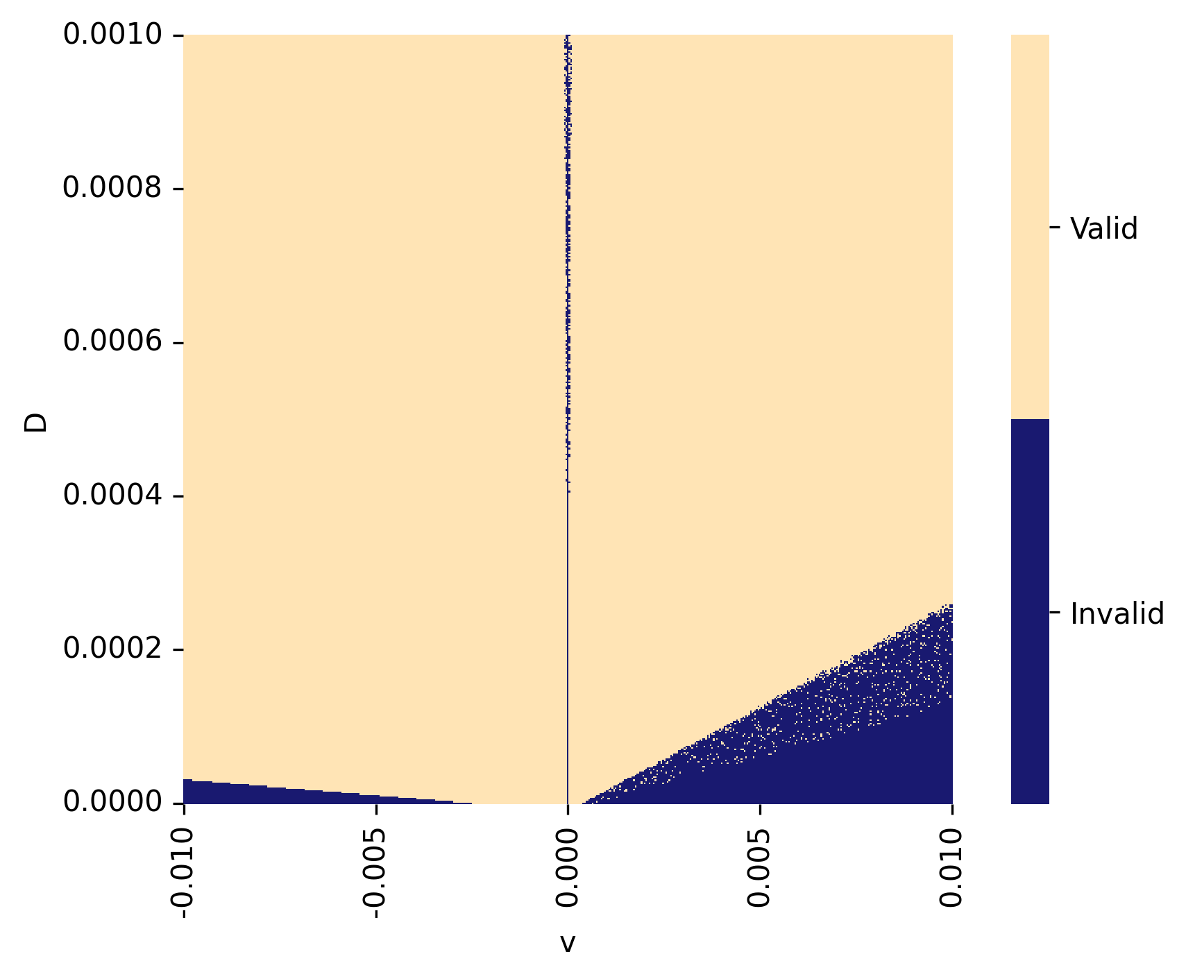
(a) No resetting

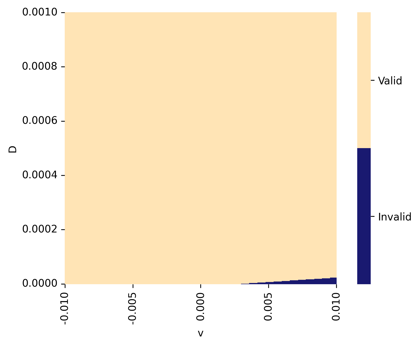
(b) With resetting, $r=(3\cdot 365)^{-1}$

Figure 1: Regions of validity of the approximated Laplace inversion with orders $m=2$, $n=3$ and for varying $v$, $D$.

The approximation appears invalid when $v=0$ for the case without resetting (Figure 1(a)). This is a consequence of Lemma 2.1, where $s$ must be strictly greater than $-v^{2}/(4D)$ for the propagator of the process without resetting, and of Step 1 of the proof of Proposition 3.4, where the $k$-th derivative of $\tilde{f}_{0}(s)$ must be computed as $s\rightarrow 0$, for $k\in\{0,1,\ldots,n+m\}$.

However, this is no longer true for the case with resetting (Figure 1(b)) because of Proposition 3.1, where $s$ must only be strictly greater than $-r$. Furthermore, for the case without resetting, the approximation is invalid for relatively low values of $D$. For the resetting case, this is only true when $v>0$.

We now measure the accuracy of the method based on the Padé approximation by comparing results to values obtained by simulation. The details of the simulations performed can be found in Section 4.2.

The first measure of accuracy considered is the area under the absolute difference between the approximated and simulated FPT densities, viz.

$$\Sigma=\dfrac{1}{2}\int_{0}^{\infty}|f_{\text{sim}}(t)-f_{m,n}(t)|\,dt,$$ (3.5)

where $f_{\text{sim}}$ is the histogram of simulated values and $f_{m,n}$ is the density obtained by inverting the Padé approximation. Thus $\Sigma\in[0,1]$ and the approximation becomes closer to the simulated values as $\Sigma$ vanishes.

Our second measure of accuracy is the relative distance between the percentiles i.e. quantiles. Denote by $Q_{m,n}(u)$ and $Q_{\text{sim}}(u)$ the quantiles at level $u\in(0,1)$ obtained by the Padé approximation and by Monte Carlo, respectively. The measure of accuracy is thus given by

$$\Phi(p)=\dfrac{|Q_{\text{sim}}(\frac{p}{100})-Q_{m,n}(\frac{p}{100})|}{Q_{\text{sim}}(\frac{p}{100})},\quad\text{for }p=0,\ldots,99.$$ (3.6)

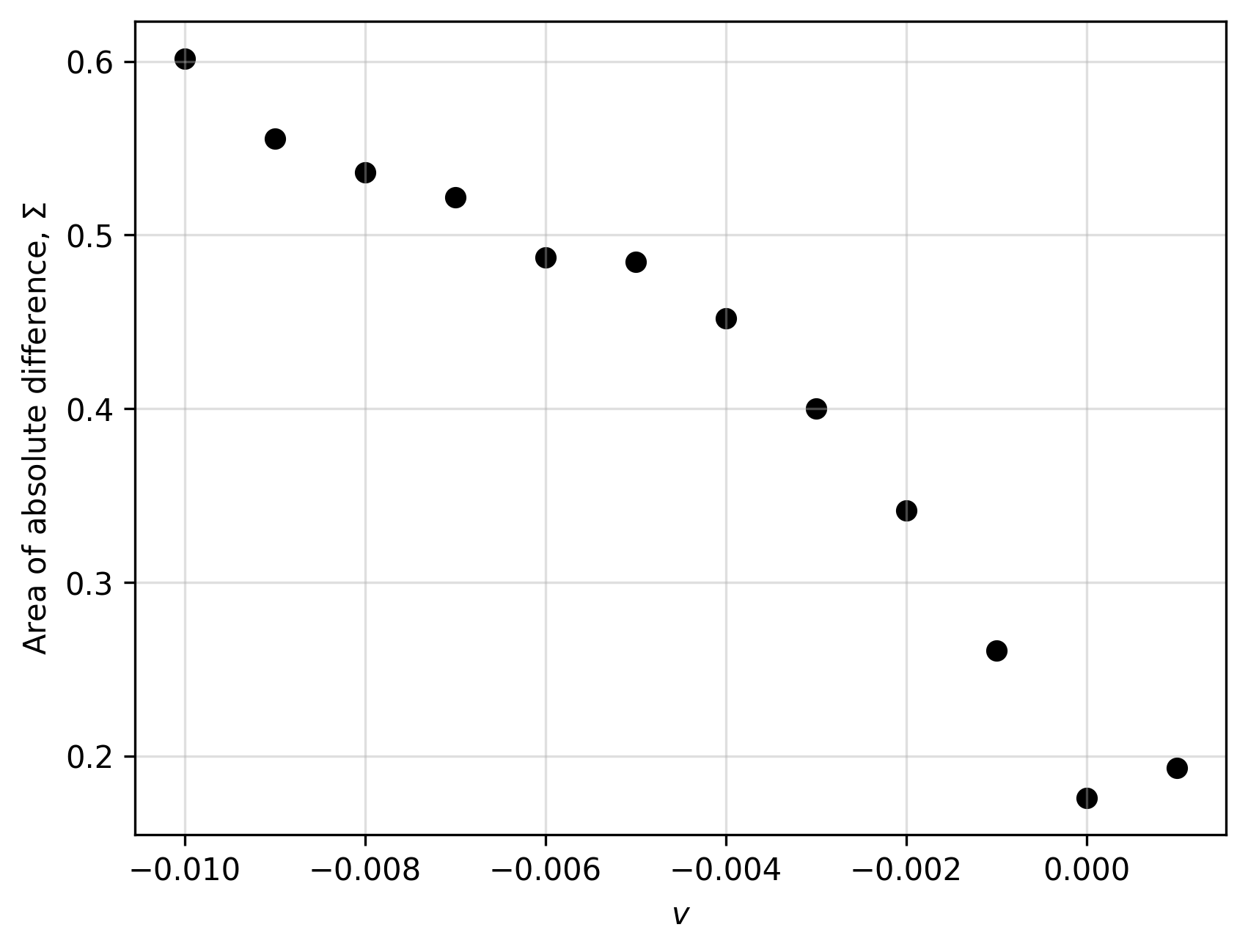
(a)

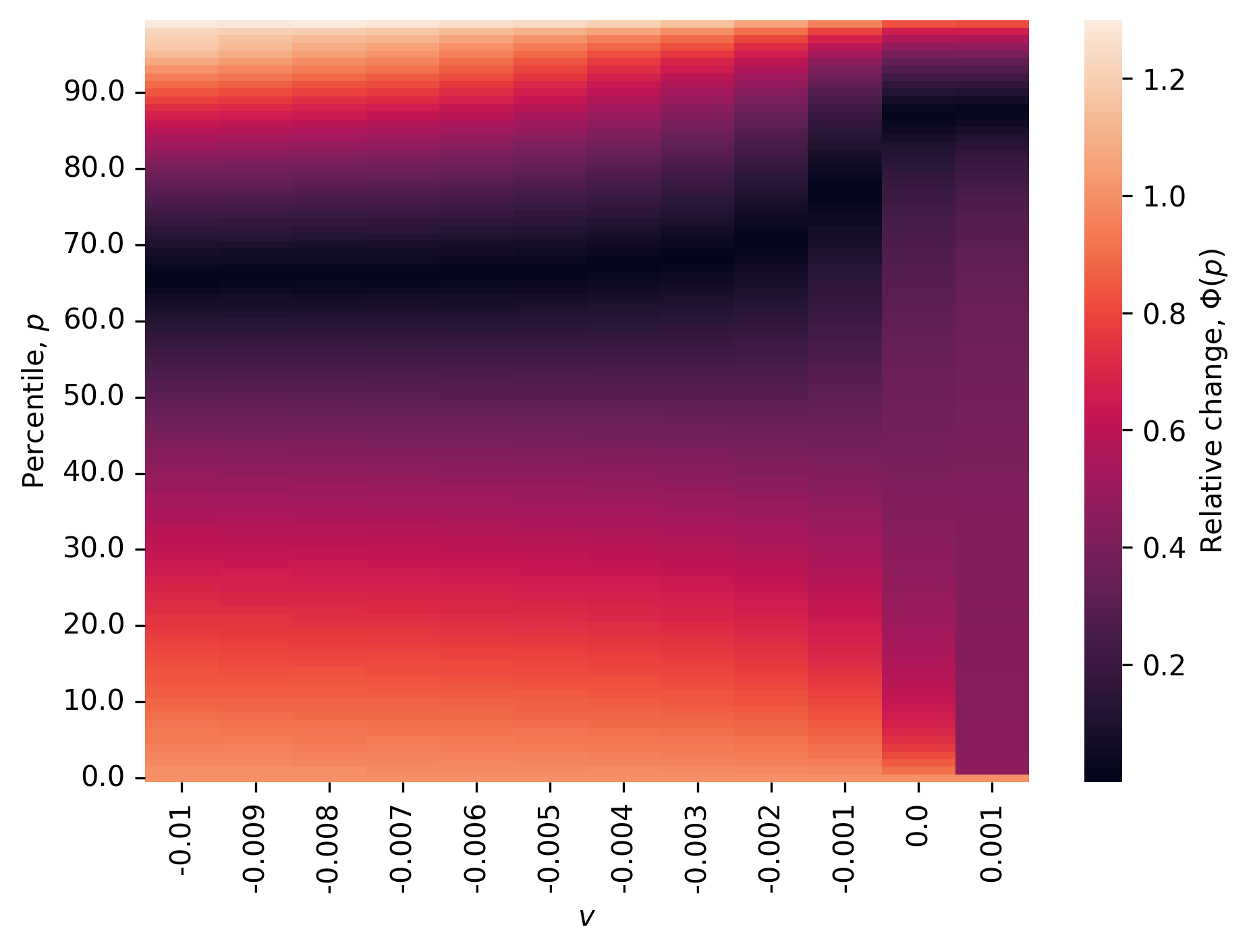
(b)

Figure 2: Area of absolute difference between densities $\Sigma$ and absolute relative error of percentiles $\Phi(p)$ for various values of $v$. $D=10^{-4}$, $r=(3\cdot 365)^{-1}$, $x_{0}=0.8$, $f_{\text{sim}}$, $10^{5}$ Monte Carlo replications with the hybrid multiresolution algorithm (Section 4.2).

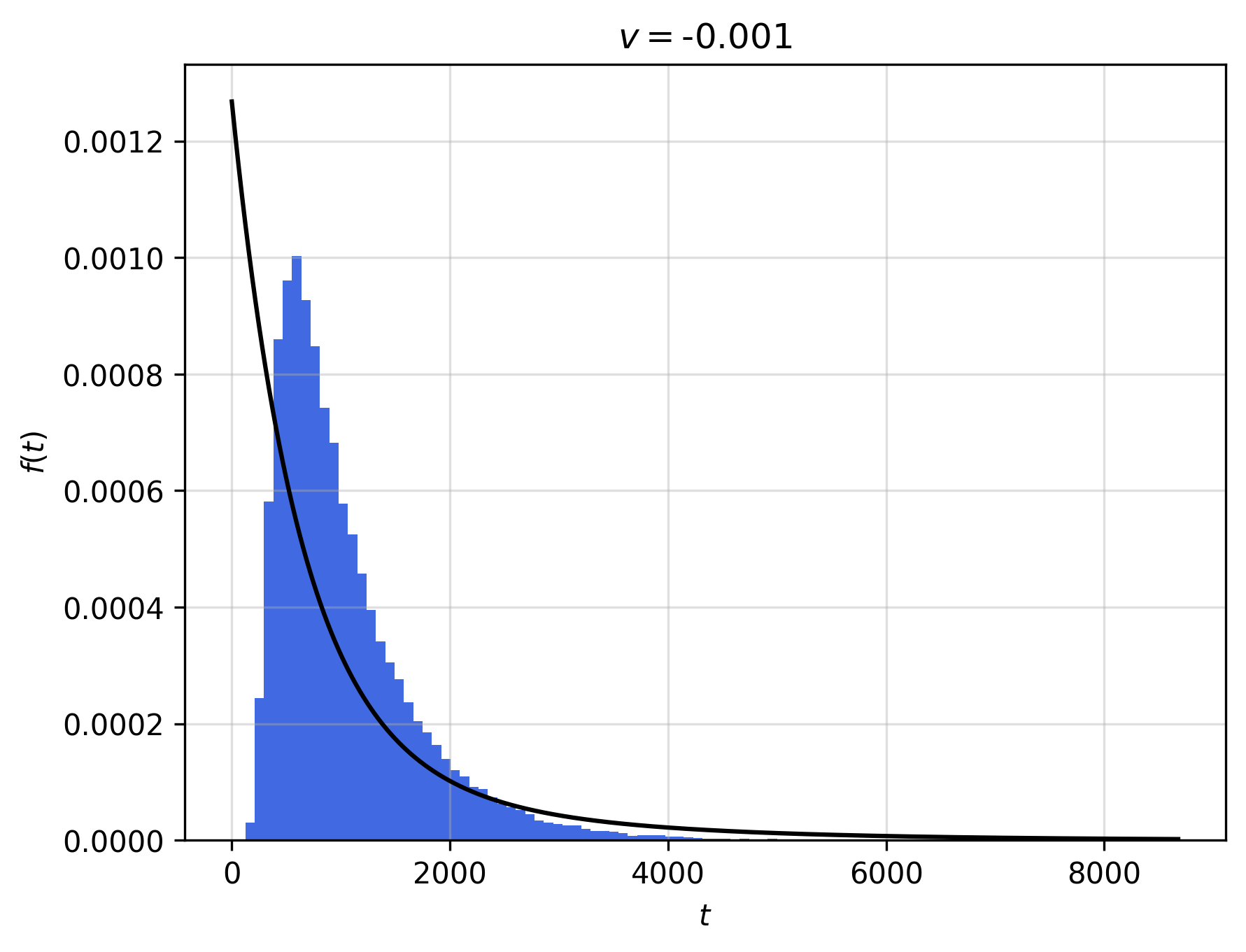
(a) $v=-0.001,\Sigma=0.261$

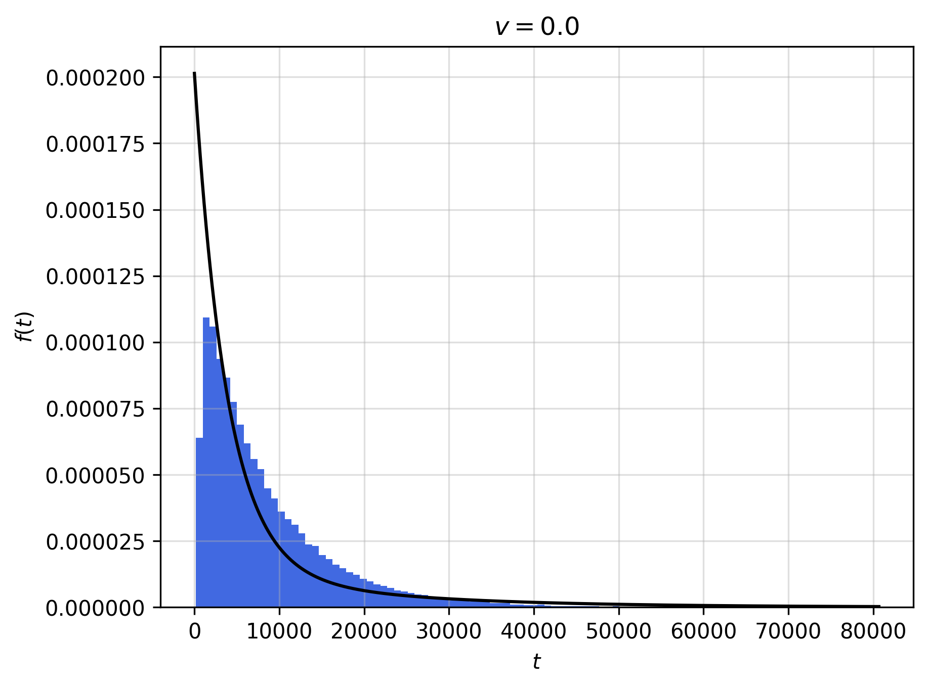
(b) $v=0.0,\Sigma=0.176$

Figure 3: Blue histograms are obtained from $10^{5}$ simulated values and black curves are obtained from Padé approximations with orders $m=2,n=3$. Points $v$, $\Sigma$ selcted from Figure 2(a).

We can observe that the values of $\Sigma$ and $\Phi(p)$, for all $p$, decrease as $v$ vanishes. In particular, $\Sigma$ reaches a minimum at $v=0$ (Figure 2(a)). For $v\geq 0$, $\Phi(p)$ is small at all $p$ (Figure 2(b)). As $v$ increases, the generated FPT increases and so the right tail of the Monte Carlo distribution increases.

Figure 3 provides two comparisons between the method based on the Padé approximation and Monte Carlo with $10^{5}$ simulations, for $v=-0.001$ with $\Sigma=0.261$ in Figure 3(a) and for $v=0$ with $\Sigma=0.176$ in Figure 3(b). We note that the Padé approximation is more accurate with low values of $\Sigma$. Larger values of $\Sigma$ lead to misleading approximations, however, those cases are fast to simulate. For larger values of $v$, Monte Carlo approximations are not feasible due to exponentially growing computing time. In this situation, it is convenient to rely on the Padé approximation.

Further comparisons with Padé approximations of higher $m$ and $n$ showed that neither the accuracy improved nor the regions of validy decreased. These results for higher orders are discussed with more details in Appendix A.

4 Monte Carlo approximation and multiresolution algorithm

Although the approximated Laplace inversion is fast to compute, sufficient accuracy can only be obtained over the right tail of the distribution (which is the important part in practice). For this reason, this section proposes an alternative approach based on the generation of the sample paths. The technique allows for arbitrary accuracy, albeit with substantial computational cost.

Generally, a selfsimilar object is one whose structure remains invariant under changes of scale. A typical illustration of a selfsimilar object is a fractal. The stochastic process $\{X_{t}\}_{t\geq 0}$ is called $h$-selfsimilar if, $\forall a>0$, $\exists h\geq 0$ such that

$$(X_{at_{1}},\ldots,X_{at_{n}})\sim(a^{h}X_{t_{1}},\ldots,a^{h}X_{t_{n}}),$$

for any $0\leq t_{1}<\ldots<t_{n}<\infty$ and $n=1,2,\ldots$; see e.g. p. 188-192 in [57]. The Wiener process is 1/2-selfsimilar.

Let $\{M_{(it^{\dagger})/n}^{\dagger}\}_{i=0,\ldots,n}$ be a general $h$-selfsimilar process over the time interval $[0,t^{\dagger}]$, where $t^{\dagger}$ is any finite time. The definition of $h$-selfsimilarity gives us directly Algorithm 1, for generating a process over an arbitrary time horizon from one over the unit time horizon.

Input: $h$, $\{M_{0},M_{1/n},M_{2/n},\ldots,M_{1}\}$

Output: $\{M^{\dagger}_{0},M^{\dagger}_{t^{\dagger}/n},M^{\dagger}_{(2t^{\dagger})/n},\ldots,M^{\dagger}_{t^{\dagger}}\}$

1 $\{M^{\dagger}_{(it^{\dagger})/n}\}_{i=0,\ldots,n}\coloneqq\emptyset$ ;

2 for $i=0\;\mathbf{to}\;n$ do

3      $M^{\dagger}_{(it^{\dagger})/n}\coloneqq(t^{\dagger})^{h}M_{i/n}$

Algorithm 1 Generation of $h$-selfsimilar process over $[0,t^{\dagger}]$

Thanks selfsimilarity or Algorithm 1, we obtain a recursive method for generating a Wiener process with arbitrary time horizon. This gives our multiresolution algorithm.

We first discuss how the multiresolution algorithm generates the Wiener process (Section 4.1). We then explain how to include a stopping condition in the algorithm so that it computes the FPT (Section 4.1.1) and how to convert the process into a Brownian motion with upper hard wall and resetting (Section 4.1.2). Finally, we combine the multiresolution algorithm with the Euler-Maruyama algorithm, in order to reduce the computational time (Section 4.2).

4.1 Multiresolution algorithm

We describe a particular strategy for generating trajectories of Wiener processes, yielding the multiresolution algorithm (following the terminology of wavelet analysis). We provide an algorithm that allows the generation of a single sample path of the Wiener process with different levels of detail or resolution. The algorithm is directly obtained from the following well-known property of the Wiener process,

$$W_{t+h}\mid(W_{t}=a,W_{t+2h}=b)\sim{\cal N}\left(\frac{a+b}{2},\frac{h}{2}\right),\;\forall t,h>0,a,b\in\mathbb{R}.$$

This property allows us to build the basic formulae (4.1)-(4.2b) for the multiresolution algorithm, that are visualized in Figures 4 and 5. This procedure allows to obtain the FPT at arbitrary accuracy. Indeed, consider the FPT

$$T_{x}=\inf\{t\geq 0\mid W_{t}\geq x\},$$

for some $x>0$, and assume that the following discretization $\{W_{nh}\}_{n=1,2,\ldots}$ of $\{W_{t}\}_{t\geq 0}$ is available, for some $h>0$ small. Then,

$$T_{h,x}=\inf\{t\geq 0\mid W_{nh}\geq x\}$$

is an overestimation of $T_{x}$, which converges to $T_{x}$ as $h\to 0$. This tells us that applying the multiresolution algorithm at increasing resolutions allows us to approximate the stopping time at any desired precision. This algorithm can be found at p. 277-279 of [49]. Although its application to FPT is suggested there, to our knowledge no applications to FPT are available.

We first consider a simple case of the multiresolution algorithm in the time interval $[0,1]$. In the algorithm, the discretized Wiener process, $\{W_{k,j}\}$, with $k,j$ nonnegative integers, is obtained through (4.1) and (4.2).

The $k$-th discretization or resolution level of the sample path is denoted $\mathbf{W}_{k}=\{W_{k,j}\}$, for $k=0,1,\ldots$.

The secondary index $j$ refers to the ordinal of each element in $\mathbf{W}_{k}$ given a certain $k$. Index $j$ ranges from $0$ to $2^{k-1}$.

At initial level $k=0$, we have

$$\mathbf{W}_{0}=\{W_{0,0},W_{0,1}\},\quad\text{where }W_{0,0}=0\text{ and }W_{0,1}\sim\mathcal{N}(0,1).$$ (4.1)

Then, the next level $k\geq 1$ is obtained by

$$W_{k,2j} =W_{k-1,j},\quad\text{for }j=0,1,\ldots,2^{k-1}$$ (4.2a)

$$W_{k,2j+1} \sim\mathcal{N}\left(\dfrac{W_{k-1,j}+W_{k-1,j+1}}{2},\dfrac{1}{2^{k+1}}\right),\quad\text{for }j=0,1,\ldots,2^{k-1}-1.$$ (4.2b)

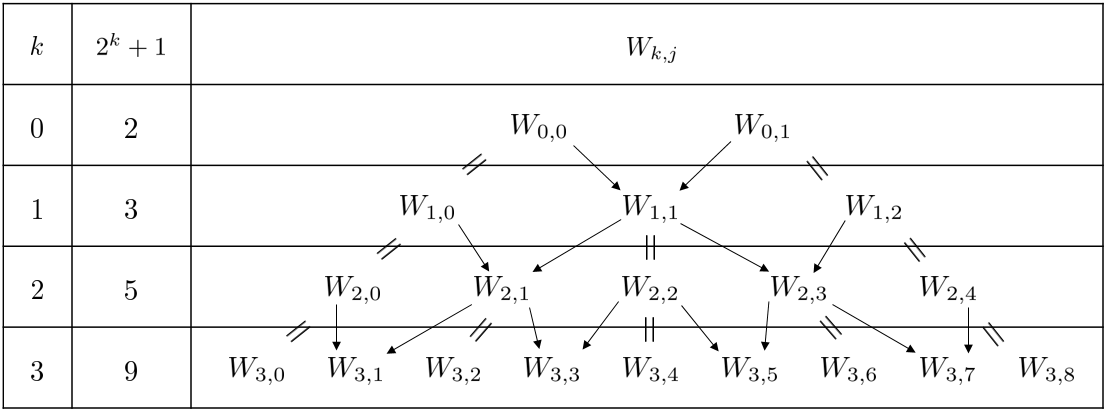
Figure 4: Resolution level $k$ and total number of variables $2^{k}+1$ (first two columns); generated random variables $W_{k,j}$ (last column). An equality indicates copying a variable from lower to higher resolution, see equation (4.2a). An arrow indicates the generation of a new variable at higher resolution with variables of lower resolution, through equation (4.2b).

The scheme for generating the discretized path of the Wiener process $\mathbf{W}_{k}$ can be visualized in Figure 4.

For $k>0$, the even indices of $j$ are copied over as the resolution increases as in equation (4.2a). The odd indices of $j$ are generated randomly using two consecutive variables from the previous resolution, as in equation (4.2b).

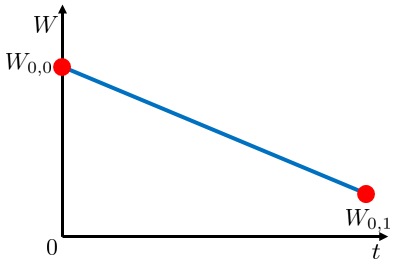
(a) $k=0$

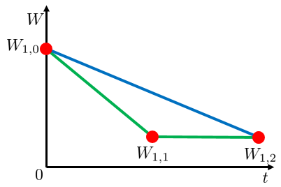
(b) $k=1$

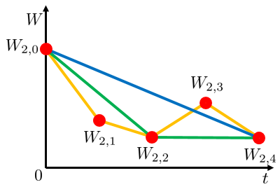
(c) $k=2$

Figure 5: Illustrations of the Wiener trajectory generated from the multiresolution algorithm: $k=0$ (blue), $k=1$ (green) and $k=2$ (orange).

Input: initial position $W_{0}$

Output: $\mathbf{W}=\{W_{0},\ldots,W_{2^{k-1}}\},\mathbf{t}=\{0,\ldots,t^{\dagger}\}$

1 $k\coloneqq 0$ ;

2 $W_{1}\coloneqq W\sim\mathcal{N}(0,1)$ ;

3 $\mathbf{W}\coloneqq\{W_{0},W_{1}\}$ ;

4 $\mathbf{t}\coloneqq\{0,1\}$ ;

5 while $\mathbf{W}$ has not reached a stopping condition do

6       $k\coloneqq k+1$ ;

7       $\mathbf{W}^{*}\coloneqq\emptyset;\quad\mathbf{t}^{*}\coloneqq\emptyset$ ;

8       for $j=0\;\mathbf{to}\;2^{k}+1$ do

9             $j^{\prime}\coloneqq\left\lfloor\dfrac{j}{2}\right\rfloor$ ;

10             if $j$ is even then

                   $W_{j}^{*}\coloneqq W_{j^{\prime}}$ ;

                    $\triangleright$ note: $W_{j^{\prime}}$ is $j^{\prime}$-th element of $\mathbf{W}$

                   $t_{j}^{*}\coloneqq t_{j^{\prime}}$ ;

                    $\triangleright$ note: $t_{j^{\prime}}$ is $j^{\prime}$-th element of $\mathbf{t}$

11                  

12             else

13                   $\mu_{int}\coloneqq\dfrac{W_{j^{\prime}}+W_{j^{\prime}+1}}{2}$ ;

14                   $\sigma^{2}_{int}\coloneqq\dfrac{1}{2^{k+1}}$ ;

15                   $W_{j}^{*}\coloneqq W\sim\mathcal{N}(\mu_{int},\sigma^{2}_{int})$;

16                   $t_{j}^{*}\coloneqq\dfrac{t_{j^{\prime}}+t_{j^{\prime}+1}}{2}$ ;

17                  

18            

19      $\mathbf{W}\coloneqq\mathbf{W}^{*}$;

20       $\mathbf{t}\coloneqq\mathbf{t}^{*}$ ;

21      

Algorithm 2 Basic multiresolution algorithm

The basic multiresolution algorithm on the time interval $[0,1]$ is implemented in Algorithm 2. This pseudocode will generate the two arrays $\mathbf{W}$ and $\mathbf{t}$, the positions and times respectively of the trajectories. The final resolution level $k$ can be arbitrarily obtained with a given stopping condition.

4.1.1 Stopping condition

We first note that the generation of the FPT requires generating sample paths with arbitrary time horizons. The $1/2$-selfsimilarity of the Wiener process allows for the use of Algorithm 1. We can thus extending the multiresolution algorithm to any time horizon $t^{\dagger}>0$.

Next, the event that the process touches the absorbing boundary is an instance of the stopping condition mentioned in Algorithm 2. For a given resolution $k$, we can record the first time in $\mathbf{t}_{k}$ at which the trajectory $\mathbf{W}_{k}$ goes below the absorbing boundary, which is the null line. This time provides an approximation to the FPT of the Wiener process.

Increasing the resolution yields finer sample paths and these intermediate variables are obtained by (4.2). Furthermore, more values in the sample path allows for finer values of FPT, this as $k$ increases, providing closer approximations to the FPT of the sample path of the Wiener process.

Consequently, these finer values mean that we must simulate more points in $\mathbf{W}_{k}$. Each new step of resolution requires generating $2^{k}$ new Gaussian variables.

An explicit condition at which we may stop the simulation can be defined by using an error threshold $\epsilon>0$. Once the time increment $\delta_{k}$ of the sample path is below $\epsilon$, we can take the FPT of $\mathbf{W}_{k}$ as the best approximate. Thus, the stopping condition to obtain the FPT time $\tau_{r}$ is

$$\tau_{r}=\inf\{t_{k,j}\in\textbf{t}_{k}\,|\,W_{k,j}<0\text{ and }\delta_{k}\leq\epsilon\}.$$ (4.3)

We define the time increments in the $k^{\text{th}}$ resolution of the multiresolution algorithm as $\delta_{k;{[0,1]}}=1/2^{k}$. See Figure 5 for a sketch showing how the number of points in the Wiener process grows with $k$. Using Algorithm 1, for a path that goes up to an arbitrary maximum time of $t^{\dagger}$, the time increments of the multiresolution are given by $\delta_{k}=t^{\dagger}/2^{k}$.

Using the definition of the time increment, note that we can now also relate time $t$ with the multiresolution indices $k,j$: $t=(jt^{\dagger})/2^{k}$.

4.1.2 Model features and resetting

Our model of Section 2.1 requires the integration of drift, resetting and hard wall in the simulation scheme. In this presentation, the indices for the Wiener trajectory will be interchangeable between $W_{k,j}$ and $W_{t}$, using the expression $t=(jt^{\dagger})/2^{k}$.

First, we generalize the Wiener process with variables $W_{t}$ to a Brownian process with variables $B_{t}$. We take a general solution to the unbounded SDE in (2.1) at the maximum simulation time $t^{\dagger}$ and an initial position at $x_{0}$,

$$B_{t^{\dagger}}=x_{0}+vt^{\dagger}+\sqrt{2D}\,W_{t^{\dagger}}.$$ (4.4)

Thus at the maximum simulation time, $B_{t^{\dagger}}$ is a normally distributed random variable with mean $\mu=x_{0}+vt^{\dagger}$ and variance $\sigma^{2}=2Dt^{\dagger}$.

With this inclusion, we can modify (4.1) and (4.2) to include parameters for drift $v$, diffusion $D$ and simulation time horizon $t^{\dagger}$. Using $k,j$ indices again and starting at $k=0$, the multiresolution algorithm for a general Wiener process starting at position $B_{0,0}=x_{0}$ is written as

$$\mathbf{B}_{0}=\{B_{0,0},B_{0,1}\},\quad\text{where }B_{0,1}\sim\mathcal{N}(x_{0}+vt^{\dagger},2Dt^{\dagger}).$$ (4.5)

Similar to (4.2), the generation of the process at the next resolution $k$ is obtained by

$$B_{k,2j} =B_{k-1,j},\quad\text{for }j=0,1,\ldots,2^{k-1},\quad\text{and}$$ (4.6a)

$$B_{k,2j+1} \sim\mathcal{N}\left(\dfrac{B_{k-1,j}+B_{k-1,j+1}}{2},\dfrac{2Dt^{\dagger}}{2^{k+1}}\right),\quad\text{for }j=0,1,\ldots,2^{k-1}-1.$$ (4.6b)

Reflection occurs when $B_{k,j}>1$, which bounds the Brownian motion between 0 and 1. Recall that the reflecting boundary is of type hard wall [11]. Hence, the individual increments of the Brownian motion are reflected back into $[0,1)$. We let process $\mathbf{B}_{k}^{\prime}$ be the reflected Brownian motion, its corresponding elements $B_{k,j}^{\prime}$ are generated using the original Brownian process $B_{k,j}$ by

$$\begin{split}B_{k,j+1}^{\prime}&=\begin{cases}B_{k,j}^{\prime}+\Delta B_{k,j},&\text{ if }B_{k,j}^{\prime}+\Delta B_{k,j}\leq 1,\\ 2-(B_{k,j}^{\prime}+\Delta B_{k,j}),&\text{ if }B_{k,j}^{\prime}+\Delta B_{k,j}>1\end{cases}\\ &=\mathrm{min}\left\{B_{k,j}^{\prime}+\Delta B_{k,j},2-(B_{k,j}^{\prime}+\Delta B_{k,j})\right\}\end{split}$$ (4.7)

where $\Delta B_{k,j}=B_{k,j+1}-B_{k,j}$.

We consider this reflected process $\mathbf{B}_{k}^{\prime}$ to check if the stopping condition (4.3) has been reached at a given resolution $k$, since it tends to the trajectory of a sample path. However, the reflected trajectory is not considered when creating finer values in the process and only the original process $\mathbf{B}_{k}$ is used when increasing the resolution. Thus, the reflected trajectory is discarded if it does not reach the stopping condition.

Finally, resetting is implemented by replacing the maximum simulation time $t^{\dagger}$ by an element from a Poisson process. Stochastic resetting is a Poisson process independent of the Brownian motion. Resetting times are exponentially distributed with a rate parameter equal to the resetting rate $r$. The Poisson process of reset times is the sequence of partial sums of i.i.d. exponentially distributed random variables

$$\mathbf{t^{\dagger}}=\{0,t_{1}^{\dagger},t_{2}^{\dagger},\ldots,t^{\dagger}_{R}\},\quad\text{where }(t^{\dagger}_{i+1}-t^{\dagger}_{i})\sim\text{Exp}(1/r),$$ (4.8)

where $R$ is the number of resets in the entire process. We can now define “reset intervals” defined by pairs of consecutive reset times: $\{(0,t^{\dagger}_{1}),(t^{\dagger}_{1},t^{\dagger}_{2}),\ldots,(t^{\dagger}_{R-1},t^{\dagger}_{R})\}$. In between each reset interval $(t^{\dagger}_{i},t^{\dagger}_{i+1})$, we generate a Brownian process using the multiresolution algorithm. This process starts at the initial position $B_{0,0}=x_{0}$ with initial time $0$ and ends at final position $B_{0,1}$ with final time $t^{\dagger}_{i+1}-t^{\dagger}_{i}$. Initial and final positions are generated in (4.5). After the generation of the process in this interval, the interval of time $(0,t^{\dagger}_{i+1}-t^{\dagger}_{i})$ is shifted by a factor of $t^{\dagger}_{i}$, resulting in the intended time interval $(t^{\dagger}_{i},t^{\dagger}_{i+1})$. This procedure of generating Brownian motions in between the reset intervals continues for all reset intervals simultaneously until the last reset interval $(t^{\dagger}_{R-1},t^{\dagger}_{R})$.

Then all the processes generated in between the reset intervals are concatenated in a sequence, which we can call $\mathbf{X}_{k}$. This is followed by implementing the reflection condition (4.7) obtaining $\mathbf{X}_{k}^{\prime}$, and finally, implementing the stopping condition (4.3) on $\mathbf{X}_{k}^{\prime}$. If the stopping condition has not been reached, $\mathbf{X}_{k}^{\prime}$ is discarded and the resolution of $\mathbf{X}_{k}$ is increased.

A limitation of this procedure is that the maximum number of resets $R$ that will be allowed is fixed in advance. We can choose an arbitrarily large $R$ corresponding to a large maximum time $t^{\dagger}_{R}$, which is similar to choosing an arbitrarily large simulation time $t^{\dagger}$ for the non-resetting case. However, this leads to higher computational effort since it generates longer Brownian trajectories.

In practice, the algorithm with resetting generates a Brownian motion within the reset intervals sequentially. The concatenated sequence $\mathbf{X}_{k}$ is generated incrementally, one reset interval after another. The algorithm has a simulation parameter $k^{\dagger}$ which is the minimum resolution required before a stochastic reset occurs. Once a reflected process in between the reset interval $(t^{\dagger}_{i},t^{\dagger}_{i+1})$ reaches $k^{\dagger}$ and has all elements above zero, it will “reset” by proceeding to generate a new Brownian process on the next reset interval $(t^{\dagger}_{i+1},t^{\dagger}_{i+2})$, starting from $B_{0,0}=x_{0}$.

Once any element of the process in between a reset interval reaches below zero, the resolution level is allowed to go above $k^{\dagger}$. The process is allowed to evolve either to reach the stopping condition (4.3) or to reach a resolution level $k^{*}$. The simulation parameter $k^{*}$ tells the maximum resolution that the Brownian trajectory can take to ensure that the simulation does not run indefinitely for any stopping condition provided. As such, $k^{*}>k^{\dagger}$.

This procedure enables the reduction of the computation cost by stopping the generation of long Brownian motion in reset intervals when $0$ has already been reached in an earlier reset interval.

4.2 Hybrid multiresolution algorithm

The multiresolution algorithm presented in the previous section has a high computational requirement. The reasons are that for the non-resetting case, we first choose an arbitrarily high time threshold, $t^{\dagger}$ and if $t^{\dagger}\gg\tau_{r}$ it would lead to a large portion of the generated trajectory not being used. However, note that one could use the approximated Laplace inversion method (Section 3.2) to choose an appropriate $t^{\dagger}$ by inspecting its right tails.

For the resetting case, recall that we apply the multiresolutional algorithm to a reset interval $(t_{i}^{\dagger},t_{i+1}^{\dagger})$, and if it does not hit the barrier up to a resolution threshold $k^{\dagger}$, we continue to the next reset interval $(t_{i+1}^{\dagger},t_{i+2}^{\dagger})$. From a computational point of view, this is problematic since we need a high resolution threshold $k^{\dagger}$ to ensure that it does not hit the barrier before going to the next interval. Also, the case where $t_{i}^{\dagger}\ll\tau_{r}$ leads to a large simulation time due to a large number of resets.

Input: $X_{0},v,D,r,\Delta t$

Output: $\tau_{r}$

1 $X\coloneqq X_{0}$;

2 $t\coloneqq 0$ ;

3 $t^{\dagger}\coloneqq t_{r}\sim\mathrm{Exp}(1/r)$ ;

4 while $X>0$ do

5       if $t\geq t^{\dagger}$ then $\triangleright$ resetting condition

6             $X\coloneqq X_{0}$ ;

7             $t\coloneqq t^{\dagger}+t_{r},\quad\text{where }t_{r}\sim\mathrm{Exp}(1/r)$

8       else

9             $X\coloneqq X+\Delta X,\quad\text{where }\Delta X\sim\mathcal{N}(v\,\Delta t,2D\,\Delta t)$ ;

10             $t\coloneqq\min\{t+\Delta t,t^{\dagger}\}$ ;

11             if $X\geq 1$ then $\triangleright$ reflection condition

12                   $X\coloneqq 2-X$

13             else if $X\leq 0$ then $\triangleright$ first passage/stopping condition

14                  $\tau_{r}\coloneqq t$

15            

16      

Algorithm 3 Euler-Maruyama algorithm for first passage

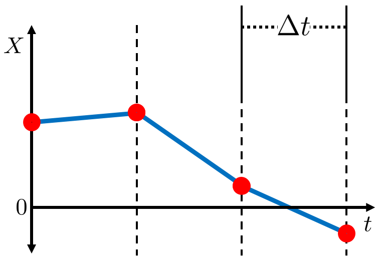
(a) Euler-Maruyama ($k=0$)

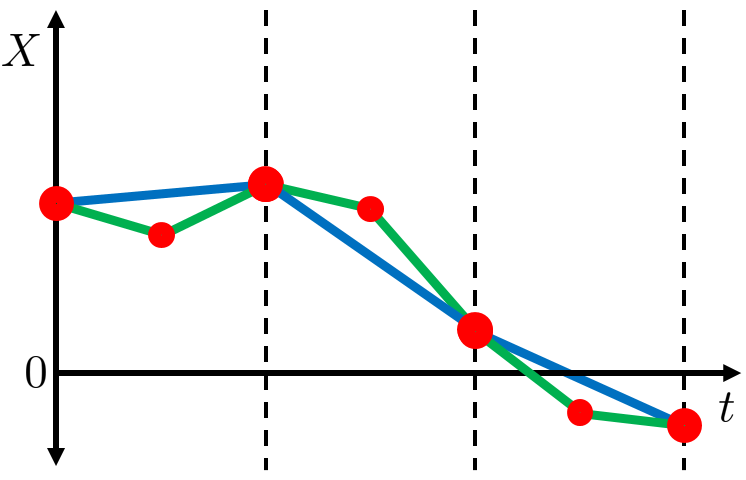
(b) $k=1$

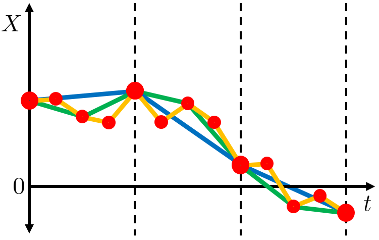
(c) $k=2$

Figure 6: Diagram showing the Wiener trajectory generated from the hybrid multiresolution algorithm. In the figures, the time increments of the Euler-Maruyama algorithm ($\Delta t$) are sketched as the separation of vertical dashed lines.

The Euler-Maruyama algorithm partially overcomes these limitations, however it tends to overestimate the FPT and it does not have an arbitrary accuracy. We propose a “hybrid algorithm” that refines the Euler-Maruyama trajectories with the multiresolution algorithm (Figure 6). In doing so, first we produce a trajectory of the Euler-Maruyama (Algorithm 3), with a time step $\Delta t$. Close to the absorbing boundary, i.e. $X<\lambda$, for some small $\lambda>0$, we use the multiresolution algorithm to refine the approximation. The details are included in Appendix E.

4.3 Results

In this section we study the performance of the pure and hybrid multiresolution algorithms in terms of accuracy, memory requirements, and speed.

First, we compare the accuracy of the pure and hybrid algorithms by comparing their simulated mean FPT with the analytical mean FPT from Proposition 2.2. As error threshold $\epsilon$ decreases, both algorithms converge to the analytical solution (Figure 7). For the hybrid, we observe that both a decrease in Euler-Maruyama time step $\Delta t$ or a decrease in $\epsilon$ lead to convergence.

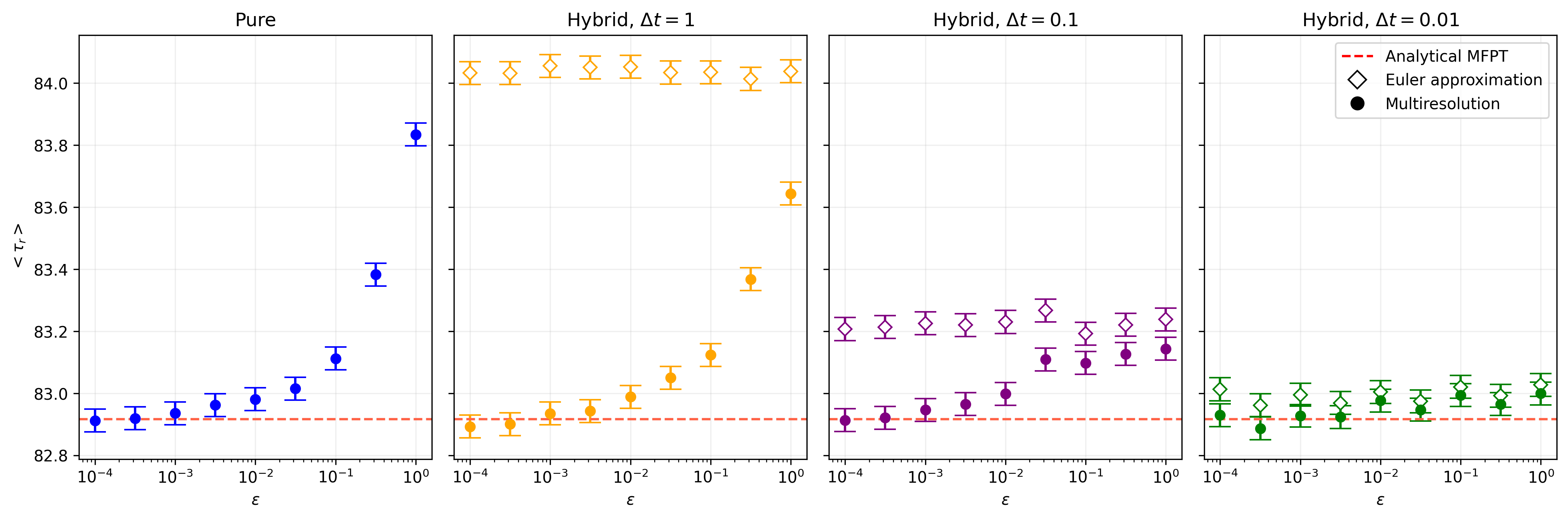
Figure 7: Pure algorithm and hybrid algorithm results with different Euler-Maruyama time steps $\Delta t$, with changing threshold $\epsilon$. $v=-10^{-2}$, $D=10^{-4}$, $r=(3\cdot 365)^{-1}$, $x_{0}=0.8$, $10^{6}$ simulations.

Next, we study the computational requirements of both algorithms. When we decrease $\epsilon$, we observe a linear increase in $<k>$, that would lead to an exponential increase in memory requirements as it is proportional to the number of points generated for each trajectory. In this sense, the hybrid outperforms the pure algorithm since it needs lesser points to reach the same accuracy (Figure 8(a)). Additionally, the hybrid outperforms the pure algorithm in terms of speed by 2 to 4 orders of magnitude (Figure 8(b)).

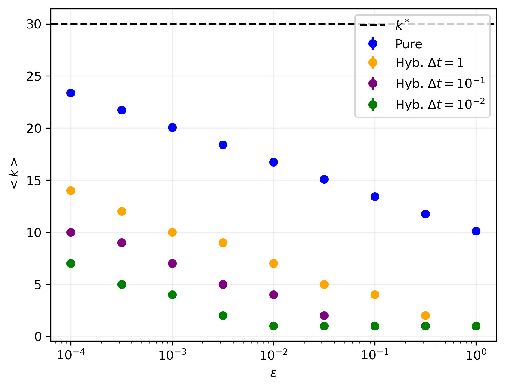
(a) $\langle k\rangle$

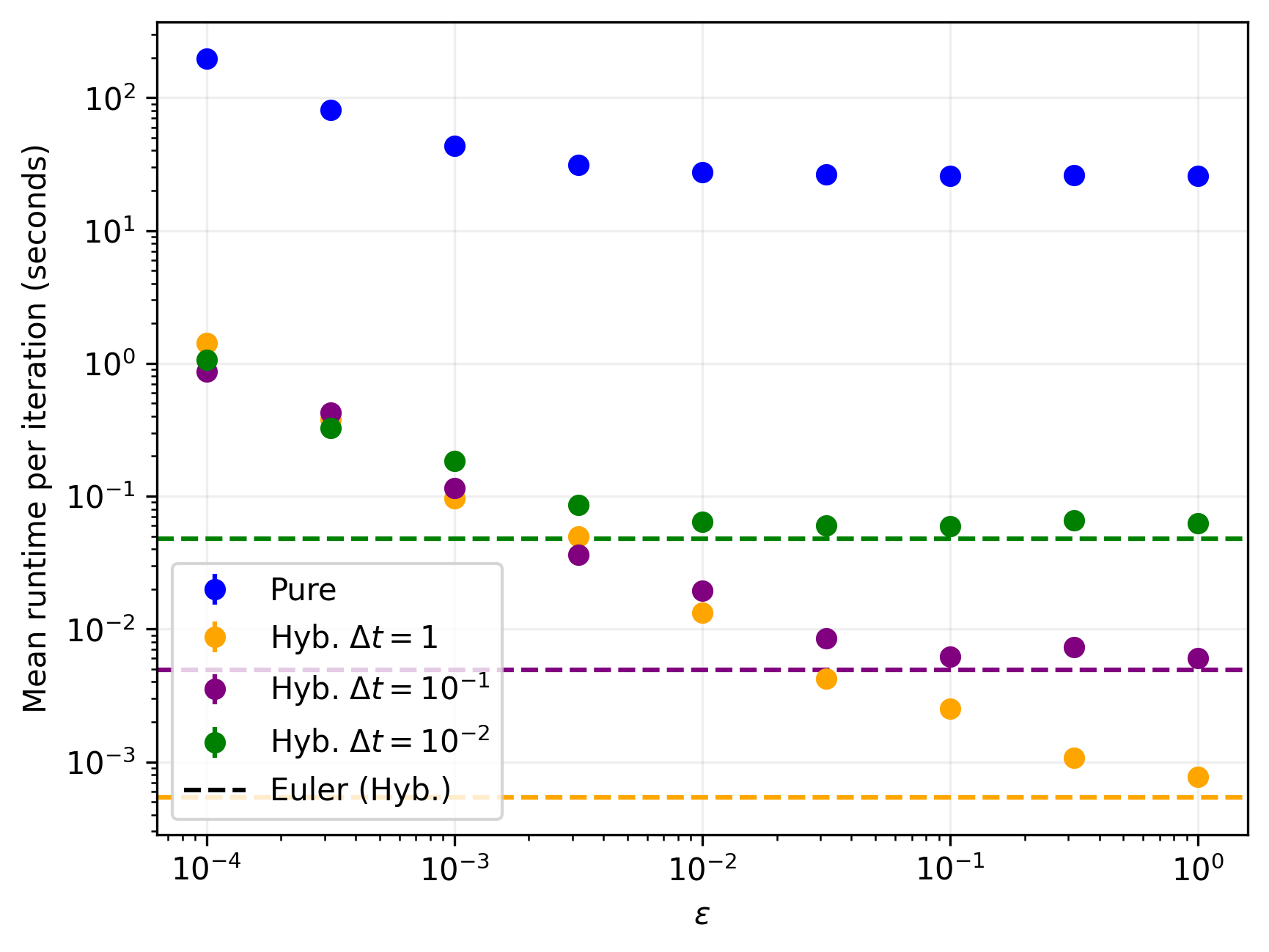
(b) $\langle t_{run}\rangle$

Figure 8: Mean resolution and runtime per iteration. Dashed lines in Subfigure 8(a) refer to the maximum $k$. Dashed lines in Subfigure 8(b) refer to the mean runtimes of the corresponding first Euler-Maruyama estimates for the hybrid algorithm.

We have observed that the hybrid outperforms the pure algorithm. However, the hybrid requires two parameters to be set, $\epsilon$ and $\Delta t$. Last, we study the impact of either parameters in terms of computational time. For all the values of $\Delta t$ we observe a region in which a decrease in $\epsilon$ is not translated to a remarkable increase in computational time. However, as $\epsilon$ is further decreased, the computational time rapidly increases by orders of magnitude. This suggests the existence of a critical value of $\epsilon$ that maximizes the trade-off between accuracy and speed.

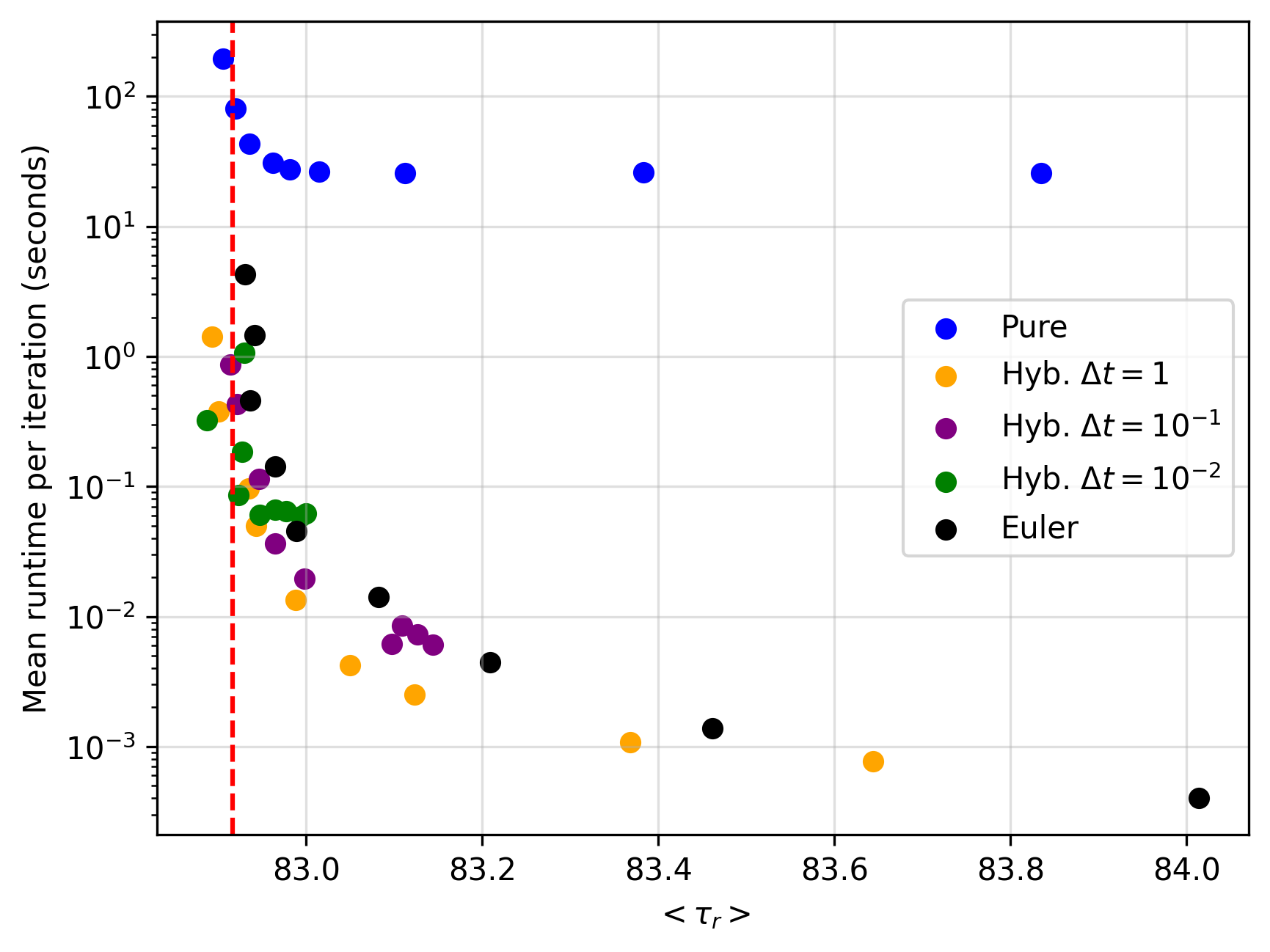
Figure 9: Comparisons between the mean FPT and the mean runtime per iteration of different simulation schemes. Pure and hybrid multiresolution simulations taken from Figure 7, Euler-Maruyama plotted simulations with varying $\Delta t$, vertical red dashed line is the analytical mean FPT.

5 Discussion

We have studied the distribution of the FPT to the null level of the drifted Brownian motion with upper hard wall barrier and Poisson resetting times. We have derived an exact formula for the mean FPT and the Laplace-transformed FPT distribution. We have also obtained an approximation for the inverse Laplace-transformed FPT distribution. Finally, we have also presented a numerical method to simulate FPTs with an arbitrary accuracy.

Using the definition of the survival function in terms of the FPT distribution, we have found a more compact expression of the mean FPT with resetting that only uses the Laplace-transformed FPT distribution without resetting [29, 30]. This is in comparison to the previously published method that used the exponential generating function for the moments in obtaining a Laplace-transformed FPT distribution with resetting [41]. Additionally, we have also provided a formal derivation of the Laplace-transformed FPT distribution.

Given that the Laplace-transformed FPT distribution is a rational function, we have proposed an approximation of the inverse Laplace transform by taking the Padé approximation and partial fraction decomposition of the expression [48].

We have determined parameter regions where the approximation is valid and accurate and we have found that the approximated inversion is generally invalid for systems with small noise, and in the case of no resetting, it is invalid when there is no bias in the process. Additionally, the accuracy of the inversion increases when FPT increases.

To overcome these limitations, we have presented the multiresolution algorithm. Given three consecutive points on a stochastic trajectory, a property of Wiener processes is that the intermediate of the three points is correlated to the first and last points [58]. The multiresolution algorithm exploits this property by generating intermediate points between intervals of the trajectory using the said expression for the correlation. Hence, the algorithm can generate finer values up to any threshold of error compared to other methods [49].

We have shown that our simulation algorithm is a valid method for generating stochastic trajectories, since the mean FPT of the simulations converges to the true mean FPT.

An issue with the Euler-Maruyama algorithm is that it overestimates the FPT by a factor proportional to $\Delta t$ [49]. The multiresolution algorithm corrects this overestimation by creating Brownian bridges in between the increments of the stochastic trajectory. Since the bridges are correlated to the endpoints of the increments, the bridge as a whole can be accepted as a valid refinement of the trajectory. This is useful for cases where certain trajectories have to be preserved but have to be increased in precision.

However, our algorithm has been shown to be slow. To increase the speed of our method, we have presented a hybrid algorithm that first approximates the FPT with Euler-Maruyama and refines the solution with the multiresolution. The hybrid algorithm is more efficient in optimizing speed and accuracy than both the Euler-Maruyama and the pure multiresolution algorithm.

We have thus given a thorough description of the distribution of the FPT of a stochastic model of drug resistance development. This distribution can be used for evaluating the survival time of a patient or the resistance development time of a pathogen. The knowledge of the full distribution can be used in the future for rare events, sensitivity analysis, and uncertainty that will guide future possible biological experiments. This work motivates future research extending the multiresolution and hybrid algorithms to other Gaussian processes, such as the Ornstein-Uhlenbeck. This process arises as a solution of Langevin’s SDE (see e.g. p. 229-230 of [57]) and it is stationary. Similar results for non-Gaussian $\alpha$-stable Lévy processes would be interesting, but more challenging to obtain.

Acknowledgements

The authors are thankful to David Ginsbourger for its invaluable contributions to this research, for his dedicated support and insightful scientific discussions.

This work was supported by the UniBE ID Grant 2021, the Ruth & Arthur Scherbarth Foundation, the Agencia Estatal de Investigación (AEI, MCI, Spain) MCIN/AEI/10.13039/ 501100011033 and Fondo Europeo de Desarrollo Regional (FEDER, UE) under Project APASOS (PID2021- 122256NB-C21$/$C22) and the María de Maeztu Program for units of Excellence in R&D, grant CEX2021- 001164-M.

Appendix A Higher approximation orders

In Proposition 3.4, the orders $(m,n)$ investigated were only $m=2$ and $n=3$, as discussed in Section 3.3. We have also investigated the behaviour of the Padé approximation at higher orders, up to total order $m+n=25$.

Figure 10: Comparisons between simulated and Padé approximated distributions, with increasing order of approximation. The black histogram is taken from Figure 3(b) and coloured curves are Padé approximations. The values of the parameters are: $v=0$, $D=10^{-4}$, $r=(3\cdot 365)^{-1}$, $x_{0}=0.8$ and $10^{5}$ simulations are done.

(a) $(m,n)$ vs. $\Sigma$

(b) $(m,n)$ vs. $\Phi(p)$

Figure 11: Area of absolute difference $\Sigma$ and relative change of percentiles $\Phi(p)$, as a function of order $(m,n)$.

Increasing the order $(m,n)$ of the approximation does not increase the accuracy, as shown by Figure 11. Figure 10 also shows that the order does not change the general behaviour of the approximation. We have also observed that only consecutive values of $m,n$ yield a valid approximation.

This result means lower orders of $(m,n)$ are a more ideal choice for improving the computational costs of the approximation since lesser derivatives of $\lim_{s\rightarrow 0}\tilde{f}^{(m+n)}(s)$ have to be computed and lesser $m+n+1$ linear equations have to be solved, as outlined in Step 1 of the proof of Proposition 3.4.

Appendix B Increase resolution

This method increases the resolution to the level of inputted, $k$ coming from a resolution of $k-1$. The function takes in two arrays $\mathbf{X}_{k-1}$ and $\mathbf{t}_{k-1}$ and returns arrays $\mathbf{X}_{k}$ and $\mathbf{t}_{k}$. This code is similar to Algorithm 2, but only for increasing the resolution one level at a time. Note that the input arrays must both have length $2^{k}+1$.

Input: $\mathbf{X},\mathbf{t},D,k,t^{\dagger}$

Output: $\mathbf{X}^{*},\mathbf{t}^{*}$

1 $\mathbf{X}^{*}\coloneqq\emptyset$ ;

2 $\mathbf{t}^{*}\coloneqq\emptyset$ ;

3 for $j=0\;\mathbf{to}\;2^{k}+1$ do

4       $j^{\prime}\coloneqq\left\lfloor\dfrac{j}{2}\right\rfloor$ ;

5       if $j$ is even then

             $X_{j}^{*}\coloneqq X_{j^{\prime}}$ ;

              $\triangleright$ note: $X_{j^{\prime}}$ is $j^{\prime}$-th element of $\mathbf{X}$

             $t_{j}^{*}\coloneqq t_{j^{\prime}}$ ;

              $\triangleright$ note: $t_{j^{\prime}}$ is $j^{\prime}$-th element of $\mathbf{t}$

6            

7       else

8             $\mu_{int}\coloneqq\dfrac{X_{j^{\prime}}+X_{j^{\prime}+1}}{2}$ ;

9             $\sigma^{2}_{int}\coloneqq\dfrac{2Dt^{\dagger}}{2^{k+1}}$ ;

10             $X_{j}^{*}\coloneqq X\sim\mathcal{N}(\mu_{int},\sigma^{2}_{int})$ ;

11             $t_{j}^{*}\coloneqq\dfrac{t_{j^{\prime}}+t_{j^{\prime}+1}}{2}$ ;

12            

13      

Algorithm 4 multires: Increase resolution from $k$ to $k+1$

Appendix C Euler-Maruyama trajectory for the hybrid algorithm

This method is similar to the Euler-Maruyama algorithm described in Algorithm 3, but modified for use in the hybrid algorithm. This code will output two arrays $\mathbf{X}^{E}$ and $\mathbf{t}^{E}$ which are Euler-Maruyama trajectories but below a position threshold $\lambda>0$. This is because above this certain threshold in the position, an absorption is unlikely to happen. Note that reflection and resetting occur in this algorithm.

Input: $X_{0},t_{0},v,D,r,\Delta t,\lambda$

Output: $\mathbf{X}^{E},\mathbf{t}^{E}$

1 $X\coloneqq X_{0}$ ;

2 $t\coloneqq t_{0}$ ;

3 $\mathbf{X}^{E}\coloneqq\emptyset$ ;

4 $\mathbf{t}^{E}\coloneqq\emptyset$ ;

5 $t^{\dagger}\coloneqq t_{r}\sim\mathrm{Exp}(1/r)$ ;

6 while $X>0$ do

7       if $t\geq t^{\dagger}$ then $\triangleright$ resetting condition

8             $X\coloneqq X_{0}$ ;

9             $t\coloneqq t^{\dagger}+t_{r},\quad\text{where }t_{r}\sim\mathrm{Exp}(1/r)$

10       else

11             $X\coloneqq X+\Delta X,\quad\text{where }\Delta X\sim\mathcal{N}(v\,\Delta t,2D\,\Delta t)$ ;

12             $t\coloneqq\min\{t+\Delta t,t^{\dagger}\}$ ;

13             if $X\geq 1$ then $\triangleright$ reflection condition

14                   $X\coloneqq 2-X$

15            

16       if $X<\lambda$ then

17             $\mathbf{append}$ $X$ to array $\mathbf{X}^{E}$ ;

18             $\mathbf{append}$ $t$ to array $\mathbf{t}^{E}$

19      

Algorithm 5 euler: Generate Euler trajectory below threshold $\lambda$

Appendix D Pure multiresolution algorithm

This code uses the multires function found in Appendix B. This algorithm generates a Brownian trajectory $\mathbf{X}_{k}$, $\mathbf{t}_{k}$ and outputs its corresponding FPT with the absorbing boundary up to an error threshold $\epsilon$.

Recall the simulation parameters $k^{\dagger}$ and $k^{*}$ that were discussed in Section 4.1.2. Parameter $k^{\dagger}$ is the minimum resolution that the trajectory must have before resetting is allowed, while $k^{*}$ is the maximum resolution before the FPT is recorded and the algorithm is stopped. Note that $k^{*}>k^{\dagger}$.

Input: $x_{0},v,D,r,\epsilon,k^{\dagger},k^{*}$

Output: $\tau_{r}$

1 $t_{0}\coloneqq 0$ ;

2 $t^{\dagger}\coloneqq t^{\prime}\sim\mathrm{Exp}(1/r)$ ;

3 while $\delta_{k}>\epsilon\,\mathbf{or}\,k<k^{*}$ do

4       $k\coloneqq 0$ ;

5       $B_{f}\coloneqq B^{\prime}\sim\mathcal{N}(x_{0}+v(t^{\dagger}-t_{0}),2D(t^{\dagger}-t_{0}))$ ;

6       $\mathbf{B}\coloneqq\{B_{0},B_{f}\}$ ;

7       $\mathbf{t}\coloneqq\{t_{0},t^{\dagger}\}$ ;

8       $\mathbf{X}\coloneqq\{x_{0}\}$ ;

9       while all $X\in\mathbf{X}>0\,\mathbf{or}\,k<k^{\dagger}$ do

10             $k\coloneqq k+1$ ;

11             $\delta_{k}\coloneqq\dfrac{t^{\dagger}}{2^{k}}$ ;

12             $\mathbf{B},\mathbf{t}\coloneqq\texttt{multires}(\mathbf{B},\mathbf{t},D,k,t^{\dagger})$ ;

13             for $j=0\;\mathbf{to}\;2^{k}$ do $\triangleright$ reflection condition

14                   $\Delta B_{j}\coloneqq B_{j+1}-B_{j}$ ;

15                   $X_{j+1}\coloneqq\mathrm{min}\left\{X_{j}+\Delta B_{j},\,2-(X_{j}+\Delta B_{j})\right\}$ ;

16                  

17            if any $X\in\mathbf{X}<0\,\mathbf{and}\,(\delta_{k}<\epsilon\,\mathbf{or}\,k>k^{*})$ then $\triangleright$ stopping condition

18                   $\tau_{r}=\inf\{t\in\mathbf{t}\,|\,X_{t}<0\}$ ;

19                   $\mathbf{break}$ loops in lines $\mathbf{3}$ and $\mathbf{9}$

20             else if $k>k^{\dagger}$ then $\triangleright$ resetting condition

21                   $t_{0}\coloneqq t^{\dagger}$ ;

22                   $t^{\dagger}\coloneqq t^{\dagger}+t^{\prime},t^{\prime}\sim\mathrm{Exp}(1/r)$ ;

23                   $\mathbf{break}$ loop in line $\mathbf{9}$ and $\mathbf{return}$ to line $\mathbf{3}$

24             else  $\triangleright$ increase resolution

25                  $\mathbf{return}$ to line $\mathbf{9}$

26            

27      

Algorithm 6 Pure multiresolution algorithm

Appendix E Hybrid multiresolution algorithm

This code uses both the multires function from Appendix B and the euler function from Appendix C. The algorithm begins by generating an Euler-Maruyama trajectory $\mathbf{X}^{E}$ and $\mathbf{t}^{E}$ below the position threshold $\lambda$. Note that the reflections and resets have occurred in the initial Euler-Maruyama trajectory already.

Input: $X_{0},v,D,r,\epsilon,\Delta t,k^{*},\lambda$

Output: $\tau_{r}$

1 $t_{0}\coloneqq 0$ ;

2 $k\coloneqq 0$ ;

3 $\mathbf{X}^{E},\mathbf{t}^{E}\coloneqq\texttt{euler}(X_{0},t_{0},v,D,r,\Delta t,\lambda)$ ;

4 $\mathbf{X}^{L}\coloneqq\emptyset$ ;

5 $\mathbf{t}^{L}\coloneqq\emptyset$ ;

6 for $i=0\;\mathbf{to}\;\text{length of array }\mathbf{X}^{E}$ do

7       if $(t^{E}_{i+1}-t^{E}_{i})\leq\Delta t$ then

8             $X_{i}^{L}\coloneqq\{X_{i}^{E},X_{i+1}^{E}\}$ ;

9             $t_{i}^{L}\coloneqq\{t_{i}^{E},t_{i+1}^{E}\}$ ;

10            

11      

12while $\delta_{k}<\epsilon$ do

13       $k\coloneqq k+1$ ;

14       $\delta_{k}\coloneqq\dfrac{t^{\dagger}}{2^{k}}$ ;

15       for $\ell=0\;\mathbf{to}\;\text{length of array }\mathbf{X}^{L}$ do

             $X^{\prime}\coloneqq X^{L}_{\ell}$ ;

              $\triangleright$ note: $X^{L}_{\ell}=\{X^{E}_{i},\ldots,X^{E}_{i+1}\}_{\ell}$

             $t^{\prime}\coloneqq t^{L}_{\ell}$ ;

              $\triangleright$ note: $t^{L}_{\ell}=\{t^{E}_{i},\ldots,t^{E}_{i+1}\}_{\ell}$

16             ${X}^{L}_{\ell},t^{L}_{\ell}\coloneqq\texttt{multires}(X^{\prime},t^{\prime},D,k,t^{\dagger})$

17      $\mathbf{X}^{M}\coloneqq\text{flattened array of }\mathbf{X}^{L}$ ;

18       $\mathbf{t}^{M}\coloneqq\text{flattened array of }\mathbf{t}^{L}$ ;

19       if any $X\in\mathbf{X}^{M}<0\;\mathbf{and}\;(\delta_{k}<\epsilon\;\mathbf{or}\;k>k^{*})$ then $\triangleright$ stopping condition

20             $\tau_{r}=\inf\{t\in\mathbf{t}^{M}\,|\,X^{M}_{t}<0\}$ ;

21             $\mathbf{break}$ loop $\mathbf{10}$

22       else  $\triangleright$ increase resolution

23            $\mathbf{return}$ to line $\mathbf{10}$

24      

Algorithm 7 Hybrid multiresolution algorithm

The loop at line 6 splits both $\mathbf{X}^{E}$ and $\mathbf{t}^{E}$ into an array of arrays $\mathbf{X}^{L}$ consisting consecutive elements of the original array, e.g. for $\mathbf{X}^{E}$: $\mathbf{X}^{L}=\{\{X^{E}_{0},X^{E}_{1}\},\{X^{E}_{1},X^{E}_{2}\},\ldots\}$. Each array element of both $\mathbf{X}^{L}$ and $\mathbf{t}^{L}$ is passed through multires and afterwards, the array of arrays is flattened back to a 1D array which is called $\mathbf{X}^{M}$ and $\mathbf{t}^{M}$, to check for the first passage and the stopping condition.

References

- [1] N. G. van Kampen, Stochastic Processes in Physics and Chemistry, 3rd Edition, North-Holland Personal Library, Elsevier, 2007.
-
[2]
X. Bian, C. Kim, G. E. Karniadakis,
111
years of Brownian motion, Soft Matter 12 (30) (2016) 6331–6346.
doi:10.1039/C6SM01153E.
URL https://pubs.rsc.org/en/content/articlelanding/2016/sm/c6sm01153e - [3] A. Libchaber, From Biology to Physics and Back: The Problem of Brownian Movement, Annual Review of Condensed Matter Physics 10 (2019) 275–293. doi:10.1146/annurev-conmatphys-031218-013318.
-
[4]
P. Romanczuk, M. Bär, W. Ebeling, B. Lindner, L. Schimansky-Geier,
Active Brownian
particles, The European Physical Journal Special Topics 202 (1) (2012)
1–162.
doi:10.1140/epjst/e2012-01529-y.
URL https://doi.org/10.1140/epjst/e2012-01529-y -
[5]
R. Gatto, B. Baumgartner,
Saddlepoint
Approximations to the Probability of Ruin in Finite Time for
the Compound Poisson Risk Process Perturbed by Diffusion,
Methodology and Computing in Applied Probability 18 (1) (2016) 217–235.
doi:10.1007/s11009-014-9412-9.
URL https://doi.org/10.1007/s11009-014-9412-9 -
[6]
R. Gatto, M. Mosimann,
Four
approaches to compute the probability of ruin in the compound Poisson
risk process with diffusion, Mathematical and Computer Modelling 55 (3)
(2012) 1169–1185.
doi:10.1016/j.mcm.2011.09.041.
URL https://www.sciencedirect.com/science/article/pii/S0895717711005899 -
[7]
P. Romanczuk, I. D. Couzin, L. Schimansky-Geier,
Collective
Motion due to Individual Escape and Pursuit Response, Physical
Review Letters 102 (1) (2009) 010602.
doi:10.1103/PhysRevLett.102.010602.
URL https://link.aps.org/doi/10.1103/PhysRevLett.102.010602 -
[8]
M. L. Woods, C. Carmona-Fontaine, C. P. Barnes, I. D. Couzin, R. Mayor, K. M.
Page,
Directional
Collective Cell Migration Emerges as a Property of Cell
Interactions, PLOS ONE 9 (9) (2014) e104969.
doi:10.1371/journal.pone.0104969.
URL https://journals.plos.org/plosone/article?id=10.1371/journal.pone.0104969 - [9] G. A. Pavliotis, Stochastic Processes and Applications: Diffusion Processes, the Fokker-Planck and Langevin Equations, 1st Edition, no. 60 in Texts in Applied Mathematics, Springer, New York, 2014.
- [10] S. Karlin, H. M. Taylor, A Second Course in Stochastic Processes, Academic Press, an imprint of Elsevier, 1981.
-
[11]
S. Redner,
A
Guide to First-Passage Processes, Cambridge University Press,
Cambridge, 2001.
doi:10.1017/CBO9780511606014.
URL https://www.cambridge.org/core/books/guide-to-firstpassage-processes/59066FD9754B42D22B028E33726D1F07 -
[12]
S. B. Yuste, K. Lindenberg,
Comment on
“Mean first passage time for anomalous diffusion”, Physical Review E
69 (3) (2004) 033101.
doi:10.1103/PhysRevE.69.033101.
URL https://link.aps.org/doi/10.1103/PhysRevE.69.033101 -
[13]
D. L. Dy, J. P. Esguerra,
First-Passage
characteristics of biased diffusion in a planar wedge, Physical Review E
88 (1) (2013) 012121.
doi:10.1103/PhysRevE.88.012121.
URL https://link.aps.org/doi/10.1103/PhysRevE.88.012121 -
[14]
R. Voituriez, O. Bénichou,
First-Passage
Statistics for Random Walks in Bounded Domains, in:
First-Passage Phenomena and Their Applications, World Scientific,
2014, pp. 145–174.
doi:10.1142/9789814590297_0007.
URL http://www.worldscientific.com/doi/abs/10.1142/9789814590297_0007 -
[15]
A. V. Skorokhod, Stochastic
Equations for Diffusion Processes in a Bounded Region, Theory of
Probability & Its Applications 6 (3) (1961) 264–274.
doi:10.1137/1106035.
URL https://epubs.siam.org/doi/10.1137/1106035 - [16] D. R. Cox, H. D. Miller, The Theory of Stochastic Processes, 1st Edition, Chapman and Hall/CRC, London, 1965.
-
[17]
A. Marcovitz, Y. Levy,
Obstacles May
Facilitate and Direct DNA Search by Proteins, Biophysical Journal
104 (9) (2013) 2042–2050.
doi:10.1016/j.bpj.2013.03.030.
URL https://www.ncbi.nlm.nih.gov/pmc/articles/PMC3647173/ -
[18]
G. Oshanin, O. Vasilyev, P. L. Krapivsky, J. Klafter,
Survival of an
evasive prey, Proceedings of the National Academy of Sciences 106 (33)
(2009) 13696–13701.
doi:10.1073/pnas.0904354106.
URL https://www.pnas.org/doi/10.1073/pnas.0904354106 -
[19]
E. Barkai, D. A. Kessler,
Transport
and the First Passage Time Problem with Application to Cold Atoms
in Optical Traps, in: First-Passage Phenomena and Their
Applications, World Scientific, 2014, pp. 502–531.
doi:10.1142/9789814590297_0020.
URL http://www.worldscientific.com/doi/abs/10.1142/9789814590297_0020 -
[20]
M. Maggiore, A. Riotto,
The
Excursion Set Theory in Cosmology, in: First-Passage Phenomena
and Their Applications, World Scientific, 2014, pp. 532–553.
doi:10.1142/9789814590297_0021.
URL http://www.worldscientific.com/doi/abs/10.1142/9789814590297_0021 -
[21]
J. Masoliver, J. Perelló,
First-Passage
and Extremes in Socio-Economic Systems, in: First-Passage
Phenomena and Their Applications, World Scientific, 2014, pp.
477–501.
doi:10.1142/9789814590297_0019.
URL http://www.worldscientific.com/doi/abs/10.1142/9789814590297_0019 -
[22]
R. Chicheportiche, J.-P. Bouchaud,
Some
Applications of First-Passage Ideas to Finance, in:
First-Passage Phenomena and Their Applications, World Scientific,
2014, pp. 447–476.
doi:10.1142/9789814590297_0018.
URL http://www.worldscientific.com/doi/abs/10.1142/9789814590297_0018 -
[23]
Y. Zhang, O. K. Dudko,
First-Passage
Processes in the Genome, Annual Review of Biophysics 45 (1) (2016)
117–134.
doi:10.1146/annurev-biophys-062215-010925.
URL https://doi.org/10.1146/annurev-biophys-062215-010925 -
[24]
J. Aguilar, B. A. García, R. Toral, S. Meloni, J. J. Ramasco,
Endemic infectious
states below the epidemic threshold and beyond herd immunity, Communications
Physics 6 (1) (2023) 1–11.
doi:10.1038/s42005-023-01302-0.
URL https://www.nature.com/articles/s42005-023-01302-0 -
[25]
S. Iyer-Biswas, A. Zilman,
First-Passage
Processes in Cellular Biology, in: Advances in Chemical Physics,
Vol. 160, John Wiley & Sons, Ltd, 2016, Ch. 5, pp. 261–306.
doi:10.1002/9781119165156.ch5.
URL https://onlinelibrary.wiley.com/doi/abs/10.1002/9781119165156.ch5 -
[26]
S. N. Majumdar, S. Sabhapandit, G. Schehr,
Dynamical
transition in the temporal relaxation of stochastic processes under
resetting, Physical Review E 91 (5) (2015) 052131.
doi:10.1103/PhysRevE.91.052131.
URL https://link.aps.org/doi/10.1103/PhysRevE.91.052131 -
[27]
M. R. Evans, S. N. Majumdar,
Diffusion with
Stochastic Resetting, Physical Review Letters 106 (16) (2011) 160601.
doi:10.1103/PhysRevLett.106.160601.
URL https://link.aps.org/doi/10.1103/PhysRevLett.106.160601 -
[28]
A. Chechkin, I. M. Sokolov,
Random
Search with Resetting: A Unified Renewal Approach, Physical
Review Letters 121 (5) (2018) 050601.
doi:10.1103/PhysRevLett.121.050601.
URL https://link.aps.org/doi/10.1103/PhysRevLett.121.050601 -
[29]
M. R. Evans, S. N. Majumdar, G. Schehr,
Stochastic resetting and
applications, Journal of Physics A: Mathematical and Theoretical 53 (19)
(2020) 193001.
doi:10.1088/1751-8121/ab7cfe.
URL https://dx.doi.org/10.1088/1751-8121/ab7cfe -
[30]
A. Pal, V. V. Prasad,
First Passage
under stochastic resetting in an interval, Physical Review E 99 (3) (2019)
032123.
doi:10.1103/PhysRevE.99.032123.
URL https://link.aps.org/doi/10.1103/PhysRevE.99.032123 -
[31]
É. Roldán, S. Gupta,
Path-integral
formalism for stochastic resetting: Exactly solved examples and shortcuts
to confinement, Physical Review E 96 (2) (2017) 022130.
doi:10.1103/PhysRevE.96.022130.
URL https://link.aps.org/doi/10.1103/PhysRevE.96.022130 -
[32]
A. Nagar, S. Gupta,
Diffusion with
Stochastic Resetting at Power-Law times, Physical Review E 93 (6)
(2016) 060102.
doi:10.1103/PhysRevE.93.060102.
URL https://link.aps.org/doi/10.1103/PhysRevE.93.060102 -
[33]
A. Pal, A. Kundu, M. R. Evans,
Diffusion under
time-dependent resetting, Journal of Physics A: Mathematical and Theoretical
49 (22) (2016) 225001.
doi:10.1088/1751-8113/49/22/225001.
URL https://dx.doi.org/10.1088/1751-8113/49/22/225001 -
[34]
L. Kusmierz, S. N. Majumdar, S. Sabhapandit, G. Schehr,
First Order
Transition for the Optimal Search Time of Lévy Flights with
Resetting, Physical Review Letters 113 (22) (2014) 220602.
doi:10.1103/PhysRevLett.113.220602.
URL https://link.aps.org/doi/10.1103/PhysRevLett.113.220602 -
[35]
J. M. Meylahn, S. Sabhapandit, H. Touchette,
Large deviations
for Markov processes with resetting, Physical Review E 92 (6) (2015)
062148.
doi:10.1103/PhysRevE.92.062148.
URL https://link.aps.org/doi/10.1103/PhysRevE.92.062148 -
[36]
G. Mercado-Vásquez, D. Boyer,
Lotka–Volterra
systems with stochastic resetting, Journal of Physics A: Mathematical and
Theoretical 51 (40) (2018) 405601.
doi:10.1088/1751-8121/aadbc0.
URL https://dx.doi.org/10.1088/1751-8121/aadbc0 -
[37]
P. C. Bressloff,