Ultimatum game: regret or fairness?

Abstract

In the ultimatum game, the challenge is to explain why responders reject non-zero offers thereby defying classical rationality. Fairness and related notions have been the main explanations so far. We explain this rejection behavior via the following principle: if the responder regrets less about losing the offer than the proposer regrets not offering the best option, the offer is rejected. This principle qualifies as a rational punishing behavior and it replaces the experimentally falsified classical rationality (the subgame perfect Nash equilibrium) that leads to accepting any non-zero offer. The principle is implemented via the transitive regret theory for probabilistic lotteries. The expected utility implementation is a limiting case of this. We show that several experimental results normally prescribed to fairness and intent-recognition can be given an alternative explanation via rational punishment; e.g. the comparison between “fair” and “superfair”, the behavior under raising the stakes etc. Hence we also propose experiments that can distinguish these two scenarios (fairness versus regret-based punishment). They assume different utilities for the proposer and responder. We focus on the mini-ultimatum version of the game and also show how it can emerge from a more general setup of the game.

I Introduction

The ultimatum game is an important experiment in behavioral economics and game theory that has been used to study human decision-making and social behavior guth . In this game, two players are given a certain amount of money $A$, and one player, the proposer ${\rm I}$, is asked to divide the money between ${\rm I}$ and the other player ${\rm II}$ (the responder). ${\rm II}$ decides whether to accept or reject the offer. If ${\rm II}$ accepts the offer, both players keep their respective shares of the money. However, if ${\rm II}$ rejects the offer, both players receive nothing. The ultimatum game has been used in a variety of research contexts, including economics, psychology, neuroscience, and sociology, to investigate questions such as how people make decisions, and how gender, individual differences, and social norms affect these decisions solnick ; solnick2 ; hessel ; chuah ; jones .

The traditional assumption in the ultimatum game is that people are rational and self-interested in the sense of sub-game perfect Nash equilibria. Hence ${\rm II}$ will accept whatever is given. Knowing about that ${\rm I}$ should offer the smallest possible amount of money. This is the only (sub-game perfect, i.e. stable) Nash equilibrium of the game. However, in practice, proposers often offer more than the minimum, and responders often reject offers that are too small; e.g. proposers offered around 30-40% of $A$, and responders tended to reject offers that were below 20-25% of $A$ guth .

Any non-zero offer is better than nothing. Why do responders reject them?

One of the main explanations for the rejection behavior is that people care about fairness whenever this serves their own interests rand ; ruffle ; straub ; fehr . This explanation assumes that when responders and proposers interchange their roles, former responders need not be willing to offer a fair amount fehr . One problem with a priori assumptions of fairness is that its general quantification is unclear. Indeed, there are experimental results showing that the simplest definition of fairness (i.e. equal split) is unstable with respect to small perturbations guthfairisunfair . This may mean that the concept of fairness is not employed by people in a sensible way. On the other hand, there are experimental results showing that an individual demonstrating rejection behavior in the ultimatum game need not behave prosocially in other games, e.g. need not cooperate in the prisoner’s dilemma game japan_rejection . Alternative existing theories for explaining the rejection behavior in the ultimatum game are reviewed in Appendix A.

Our study posits that rejection can be a rational punishment in the long run if ${\rm II}$ is trying to force ${\rm I}$ to provide better options. Once rejecting means that ${\rm II}$ sacrifices short-term rationality, there is a requirement for long-term rationality: the rejection is meaningful only when ${\rm II}$ regrets about losing the offered (smallest) amount less than ${\rm I}$ regrets about not offering a larger amount. Here, regret is understood as referring to the generalized expected utility theory for comparing probabilistic lotteries developed in savage1951 ; bell ; loomes_sugden , and recently advanced in we_regret . Ref. we_regret demonstrated that regret theory can be reconciled with basic principles of rationality, such as stochastic dominance and transitivity. Ref. we_regret also shows that the regret theory can solve the classical difficulties of the expected utility theory. In particular, it can solve Allais’ paradox, because the regret theory generally does not hold the sure thing principle we_regret , and it can solve Savage’s omelet paradox since the regret theory is a counter-factual mean of comparing two (or more) probabilistic lotteries we_regret . Once regret is a rational mean of comparing agent’s different actions with each other, it differs conceptually from envy, which is concerned with things beyond one’s control.

We show that several experimental results in the ultimatum game that are usually attributed to fairness can be given an alternative interpretation via regret-based rational punishment. This includes the following effects. (i) The very definition of fair division, which for equal utilities of ${\rm I}$ and ${\rm II}$ amounts to dividing the initial sum $A$ over two halves. (ii) Comparison between unfair/fair and unfair/superfair offers. (iii) Behavior changes (or lack thereof) under increasing stakes, i.e. proportionally increasing both the overall divided sum $A$ and the magnitudes of offers. In all these cases, regret-based punishment and fairness predict similar results only for identical utilities of ${\rm I}$ and ${\rm II}$. Their predictions are markedly different for different utilities. The mechanism behind this difference is that the richer agent can endure more losses and hence demand more, whereas according to the fairness theory, the richer agent will likely continue promoting fairness. At the very least, this is the case when the fairness is supplemented with intention recognition, as was suggested for explaining (ii) via fairness falk .

The rest of this paper is organized as follows. The next section reminds the ultimatum game and its Nash equilibrium. Section III reformulates the ultimatum game in terms of probabilistic lotteries and shows how to apply the regret theory. The ultimatum game with two outcomes (mini-ultimatum game) is studied in section IV. Here we study in detail the similarities between assuming fairness and rational punishment. Section V studies the ultimatum game for three or more offers and discusses in which sense the optimal three-offer game is reduced to the optimal two-offer game. We summarize our results in the last section.

II The ultimatum game and its Nash equilibrium

We specify the rules of the ultimatum game for two offers. This is sometimes called the mini-ultimatum game bolton_zwick ; population ; gale ; falk . This assumption is sufficient for the traditional solution. In our regret-based solution, the number of offers can be arbitrary, but the two outcomes are the minimal situation to start from. There are two players ${\rm I}$ and ${\rm II}$ and a certain amount of money $A$. Now ${\rm I}$ offers to ${\rm II}$ either $A-a_{0}$ (action $0$) or $A-a_{1}$ (action $1$):

$$A>a_{0}>a_{1}.$$ (1)

${\rm II}$ can accept any of these offers or reject them. Money is lost in the latter case: neither ${\rm I}$ nor ${\rm II}$ receives anything. In more detail, we can design this as a sequential game myerson , where ${\rm II}$ has three options: $({\rm acc},{\rm acc})$ (accept if $1$ or $0$), $({\rm acc},{\rm rej})$ (accept if $1$, reject if $0$), and $({\rm rej},{\rm rej})$ (reject if $1$ or $0$). The outcomes can be written as follows:

(5)

This table makes clear that there are two Nash equilibrium points here: $[0,({\rm acc},{\rm acc})]$ and $[1,({\rm acc},{\rm rej})]$. However, $[1,({\rm acc},{\rm rej})]$ is not subgame perfect myerson , i.e. acting ${\rm rej}$ in response to $0$ means that ${\rm II}$ looses money. Put differently, by declaring $({\rm acc},{\rm rej})$, ${\rm II}$ makes a non-credible threat. Thus, people who act $({\rm acc},{\rm rej})$ (as it frequently happens in experiments guth ) do not follow the subgame perfect Nash equilibrium myerson .

III The ultimatum game reformulated via regret

III.1 Lotteries and utilities

We start with a reformulation of the ultimatum game, where the number of divisions (offers) by ${\rm I}$ is finite and equals $n+1$: within each offer ${\rm I}$ keeps $a_{k}$ $ and gives $A-a_{k}$ $ to ${\rm II}$:

$$A>a_{0}>...>a_{n}>0.$$ (6)

Each $a_{k}$ in (6) is offered by ${\rm I}$ with prior probability $\pi_{k}\geq 0$: $\sum_{i=0}^{n}\pi_{i}=1$.

${\rm II}$ will have two options: either accept whatever is given or accept the offer $A-a_{k}$ with (conditional) probability $p_{k}$:

$$p_{0}\leq p_{1}\leq...\leq p_{n}=1.$$ (7)

The ordering in (7) is a consequence of (6); the last condition $p_{n}=1$ means that the best possible option for ${\rm II}$ is never rejected. We emphasize that this assumption of always accepting $a_{n}$ is non-trivial. We shall denote:

$$\hat{a}\equiv\{a_{i}\}_{i=0}^{n},\quad\hat{p}\equiv\{p_{i}\}_{i=0}^{n},\quad\hat{\pi}\equiv\{\pi_{i}\}_{i=0}^{n}.$$ (8)

Hence ${\rm II}$ chooses between two lotteries:

$${\rm II}_{\rm acc}=\begin{pmatrix}A-a_{0}&A-a_{1}&...&A-a_{n}\\ \pi_{0}&\pi_{1}&...&\pi_{n}\end{pmatrix},\qquad{\rm II}_{\rm rej}=\begin{pmatrix}A-a_{0}&A-a_{1}&...&A-a_{n}&0\\ p_{0}\pi_{0}&p_{1}\pi_{1}&...&p_{n}\pi_{n}&1-\sum_{i=0}^{n}p_{i}\pi_{i}\end{pmatrix}.$$ (9)

Note that the outcomes in ${\rm II}_{\rm acc}$ and ${\rm II}_{\rm rej}$ are independent of each other.

${\rm I}$ faces a choice between the following lotteries:

$${\rm I}_{n}=\begin{pmatrix}a_{n}\\ 1\end{pmatrix}\qquad{\rm I}_{0}=\begin{pmatrix}a_{0}&a_{1}&...&a_{n}&0\\ p_{0}\pi_{0}&p_{1}\pi_{1}&...&p_{n}\pi_{n}&1-\sum_{i=0}^{n}p_{i}\pi_{i}\end{pmatrix},$$ (10)

where ${\rm I}_{n}$ means offering ${\rm II}$ the best possible (for ${\rm II}$) outcome, while ${\rm I}_{0}$ relates to ${\rm II}_{\rm rej}$ in (9).

Each monetary outcome in (9, 10) has its utility $u(x)$ which is a non-decreasing function of $x$. We assume $u(0)=0$ without loss of generality. We assume that both ${\rm I}$ and ${\rm II}$ have the same utility function; this assumption will be revised later.

III.2 Regret and its calculation

We start with $\rho_{\rm II}({\rm II}_{\rm acc};{\rm II}_{\rm rej}\to A-a_{k})$ which is the regret experienced by ${\rm II}$ about not choosing ${\rm II}_{\rm acc}$, provided that ${\rm II}_{\rm rej}$ was chosen and the outcome $A-a_{k}$ has been realized. This quantity is defined as follows we_regret :

$$\rho_{\rm II}({\rm II}_{\rm acc};{\rm II}_{\rm rej}\to A-a_{k})=\sum_{l=0}^{n}\pi_{l}f[u(A-a_{l})-u(A-a_{k})],$$ (11)

$$\rho_{\rm II}({\rm II}_{\rm acc};{\rm II}_{\rm rej}\to 0)=\sum_{l=0}^{n}\pi_{l}f[u(A-a_{l})].$$ (12)

Indeed, since it is not known which outcome would have been realized within ${\rm II}_{\rm acc}$ all its outcomes enter into (12) with their probabilities. The function $f[x]$ in (12) compares different outcomes; hence it naturally holds we_regret :

$$f(x\geq 0)\geq 0,\qquad f(x\leq 0)\leq 0,\qquad f(0)=0.$$ (13)

Generally, $f[x]$ accounts for both regret and appreciation. We get a pure regret (appreciation) if $f[x\leq 0]=0$ ($f[x\geq 0]=0$).

Mean regret of not choosing ${\rm II}_{\rm acc}$ thus reads

$$\rho_{\rm II}({\rm II}_{\rm acc};{\rm II}_{\rm rej})=\sum_{k=0}^{n}p_{k}\pi_{k}\rho_{\rm II}({\rm II}_{\rm acc};{\rm II}_{\rm rej}\to A-a_{k})+\Big{(}1-\sum_{l=0}^{n}p_{l}\pi_{l}\Big{)}\rho_{\rm II}({\rm II}_{\rm acc};{\rm II}_{\rm rej}\to 0).$$ (14)

Now $\rho_{\rm II}({\rm II}_{\rm rej};{\rm II}_{\rm acc})$ is calculated in the same way assuming that ${\rm II}_{\rm acc}$ was taken etc. To decide which one, ${\rm II}_{\rm rej}$ or ${\rm II}_{\rm acc}$ was eventually worth taking, we look at the difference we_regret :

$$R_{\rm II} = \rho_{\rm II}({\rm II}_{\rm acc};{\rm II}_{\rm rej})-\rho_{\rm II}({\rm II}_{\rm rej};{\rm II}_{\rm acc})$$ (15)

$$= \Big{(}1-\sum_{i=0}^{n}p_{i}\pi_{i}\Big{)}\sum_{k=0}^{n}\pi_{k}g[u(A-a_{k})]+\sum_{0\leq i<j\leq n}(p_{j}-p_{i})\pi_{i}\pi_{j}g[u(A-a_{i})-u(A-a_{j})],$$ (16)

where we denoted [cf. (13)]:

$$g[x]\equiv f[x]-f[-x],$$ (19)

$$g[x]=-g[-x],$$

$$g[x]\geq g[y]\quad{\rm for}\quad x\geq y.$$

$g[x]$ is the main regret function we shall work with.

Likewise, we calculate from (10) for ${\rm I}$:

$$R_{{\rm I}}=\rho_{{\rm I}}({\rm I}_{n};{\rm I}_{0})-\rho_{{\rm I}}({\rm I}_{0};{\rm I}_{n})=\sum_{i=0}^{n}p_{i}\pi_{i}g[u(a_{n})-u(a_{i})]+\Big{(}1-\sum_{i=0}^{n}p_{i}\pi_{i}\Big{)}g[u(a_{n})],$$ (20)

where we assumed that ${\rm I}$ and ${\rm II}$ have the same regret function $g[x]$ in (26).

III.3 The solution

Note from (9) that every positive outcome in ${\rm II}_{\rm acc}$ have a larger probability than the same outcome in ${\rm II}_{\rm rej}$, i.e. . the probabilities in ${\rm II}_{\rm acc}$ stochastically dominate those in ${\rm II}_{\rm rej}$. This leads from (16–19) in we_regret to:

$$R_{\rm II}>0,$$ (21)

i.e. when taking ${\rm II}_{\rm acc}$ one rejects less than taking ${\rm II}_{\rm rej}$: the short-term rationality dictates choosing ${\rm II}_{\rm acc}$. ${\rm II}$ decides to sacrifice this by acting ${\rm II}_{\rm rej}$. However, long-term rationality still demands that ${\rm I}$ regrets more for not offering $a_{n}$, than ${\rm II}$ regrets for rejecting. Only under this condition, ${\rm II}$ can hope that the rejection will force ${\rm I}$ to change the offer because only under this condition the rejection by ${\rm II}$ will have a chance to be a sustainable action. This situation can be described as follows:

$${\rm II}{\rm~{}wins~{}over~{}}{\rm I}~{}{\rm if}~{}0<R_{{\rm II}}<R_{{\rm I}},$$ (22)

$${\rm I}{\rm~{}wins~{}over~{}}{\rm II}~{}{\rm if}~{}R_{{\rm II}}>R_{{\rm I}}.$$ (23)

III.4 Regret function

The simplest choice of the regret function is

$$g[x]\propto x,$$ (24)

and (16–20) reduce to difference between expected utilities ${\rm EU}$ of separate lotteries, e.g.

$$R_{{\rm II}}={\rm EU}({\rm II}_{\rm acc})-{\rm EU}({\rm II}_{\rm rej})=\sum_{l=0}^{n}\pi_{l}u(A-a_{l})-\sum_{l=0}^{n}\pi_{l}p_{l}u(A-a_{l}).$$ (25)

We shall see below the expected utility version of the theory is simple and can produce useful results, though it is not always sufficiently non-trivial; cf. Appendix B.

Modulo an affine transformation, $f[x]\to af[x]+b$ ($a>0$) of $f[x]$, there is only one regret function $g(x)$ which ensures that pairwise comparison between lotteries holds transitivity we_regret :

$$g[x]=\sinh\left[{x}/{\beta}\right],\quad\beta>0,$$ (26)

where $\beta>0$ is a parameter. We revert to (24) for $\beta\to\infty$. The intuitive meaning of (26) is explained in Appendix C.

IV Mini-ultimatum game: two offers

We focus on the mini-ultimatum case $n=1$, where there are two offers only bolton_zwick ; population ; gale . Now $p_{0}<1$, $p_{1}=1$, $\pi_{0}+\pi_{1}=1$, while in the last sum of (16) only the term with $i=0$ and $j=1$ survives. Condition (22) (i.e. ${\rm II}$ wins) amounts from (16, 20) to

$$\pi_{0}\left(g[u(A-a_{0})]-g[u(A-a_{1})]+g[u(A-a_{1})-u(A-a_{0})]\right)$$

$$< g[u(a_{1})]+\frac{p_{0}}{1-p_{0}}g[u(a_{1})-u(a_{0})]-g[u(A-a_{1})]+g[u(A-a_{1})-u(A-a_{0})].$$ (27)

For the expected utility situation (24) we get from (27)

$$u(a_{1})-u(A-a_{0})>\frac{p_{0}}{1-p_{0}}(u(a_{0})-u(a_{1})).$$ (28)

It is seen that (28) holds $u(a_{1})>u(A-a_{0})$, i.e. $a_{1}+a_{0}>A$ taking into account that $u(x)$ is monotonic function. If this condition holds, $p_{0}$ can be taken sufficiently small so that (28) holds. Thus ${\rm II}$ wins for $a_{1}+a_{0}>A$, while ${\rm I}$ wins for $a_{1}+a_{0}<A$. Now $\pi_{0}$ equals either $0$ or $1$.

Let us turn to the more general case (26). Employing (26) and standard relations

$$\sinh x-\sinh y=2\sinh\frac{x-y}{2}\cosh\frac{x+y}{2},\quad\sinh x=2\sinh\frac{x}{2}\cosh\frac{x}{2},$$ (29)

$$\cosh x-\cosh y=2\sinh\frac{x-y}{2}\sinh\frac{x+y}{2},$$ (30)

we find for (27):

$$\kappa\equiv-g[u(A-a_{0})]+g[u(A-a_{1})]-g[u(A-a_{1})-u(A-a_{0})]$$

$$=4\sinh\frac{u(A-a_{1})-u(A-a_{0})}{2\beta}\sinh\frac{u(A-a_{0})}{2\beta}\sinh\frac{u(A-a_{1})}{2\beta}\geq 0.$$ (31)

Recalling that $a_{0}>a_{1}$, while $u(x)$ and $g(x)$ are monotonously increasing, we see that Eqs. (27–31) lead to two possibilities analyzed below.

IV.1 ${\rm II}$ wins over ${\rm I}$

If in (27) we have

$$0<g[u(a_{1})]-g[u(A-a_{1})]+g[u(A-a_{1})-u(A-a_{0})],$$ (32)

then ${\rm II}$ can choose the probability $p=p_{0}$ from

$$p_{0}<\frac{g[u(a_{1})]-g[u(A-a_{1})]+g[u(A-a_{1})-u(A-a_{0})]}{g[u(a_{1})]-g[u(A-a_{1})]+g[u(A-a_{1})-u(A-a_{0})]+g[u(a_{0})-u(a_{1})]}<1,$$ (33)

so that ${\rm I}$ regrets more for any choice of $1\geq\pi_{0}\geq 0$, i.e. (27) holds. Thus, under condition (32), ${\rm II}$ can force ${\rm I}$ into proposing $a_{1}$. Note that the actual value of $p$ is not important provided that it holds (33) because ${\rm I}$ is now expected to offer $a_{1}$ with probability $1$, i.e. ${\rm II}$ has nothing to reject. As follows from (6) and the monotonicity of $g[u(x)]$ as a function of $x$, condition (32) does hold for

$$a_{1}>A/2.$$ (34)

The meaning of (34) is that even in the worst case, ${\rm I}$ does not offer less than the half of the money. And ${\rm I}$ is punished for this, because now ${\rm II}$ can ensure that for any choice of $\pi_{0}$, the regret of ${\rm I}$ is larger provided that (33) is satisfied.

IV.2 ${\rm I}$ wins over ${\rm II}$

For $a_{1}<A/2$ it is possible that (32) is inverted:

$$0>g[u(a_{1})]-g[u(A-a_{1})]+g[u(A-a_{1})-u(A-a_{0})].$$ (35)

Now ${\rm I}$ can make $\pi_{0}$ sufficiently small and invert (27) for any $p_{0}$. To this end, it is needed that [cf. (31)]

$$\pi_{0}<\pi_{c}=1+\frac{g[u(A-a_{0})]-g[u(a_{1})]}{\kappa}.$$ (36)

Thus, if (36) holds, then ${\rm II}$ is not able to force ${\rm I}$ to regretting the action of not giving the best option $a_{1}$ to ${\rm II}$. Then ${\rm II}$ will just accept whatever is given. The situation is now in equilibrium since ${\rm I}$ is well-motivated to act with probability $\pi_{0}$ close but smaller than $\pi_{c}$. Using $\pi_{0}>\pi_{c}$ means that ${\rm II}$ will force ${\rm I}$ into regret, while $\pi_{0}$ substantially lower than $\pi_{c}$ means that ${\rm I}$ looses utility.

Note from (36) that $\pi_{c}\geq 1$ for

$$g[u(a_{1})]\leq g[u(A-a_{0})],~{}~{}{\rm i.e.}~{}~{}a_{1}+a_{0}\leq A.$$ (37)

Under the last condition in (37), ${\rm II}$ cannot force ${\rm I}$ into regret and ${\rm I}$ always employs the best option $a$ (i.e. $\pi=1<\pi_{c}$), where the outcome for ${\rm I}$ is the largest one. Taken together with $a_{1}<A/2$, condition $a_{1}+a_{0}>A$ has a transparent meaning: If the amount to which ${\rm II}$ agrees with probability one is too large (e.g. $a_{1}\to 0$), ${\rm I}$ can punish ${\rm II}$ by getting almost the whole money, i.e. $a_{0}\to A$ under (37).

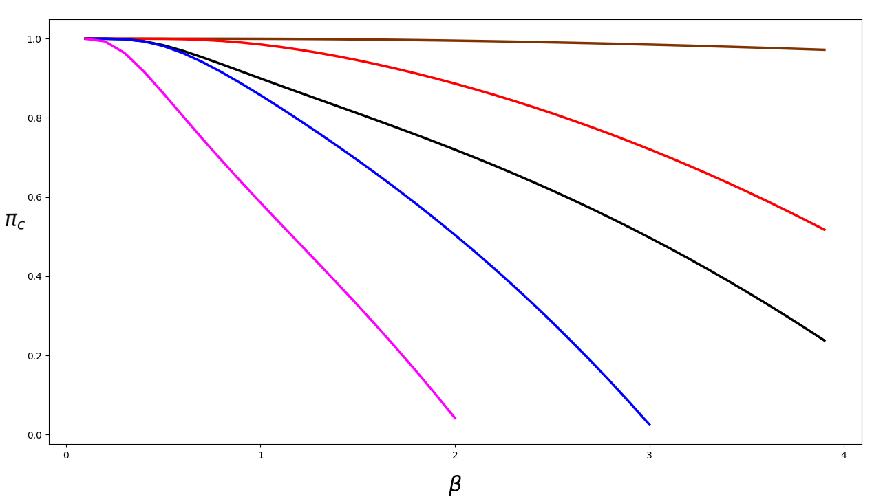
Figure 1: The critical probability $\pi_{c}$ (given by (36)) versus $\beta$ for $A=10$ and $u(x)=x$ (linear utility). Parameters of the curves are as follows (from top to bottom): brown $a_{0}=8.1$, $a_{1}=2$; red $a_{0}=8.1$, $a_{1}=3$; black $a_{0}=7.1$, $a_{1}=4$; blue $a_{0}=8.1$, $a_{1}=4$; magenta $a_{0}=8.1$, $a_{1}=4.5$. $\pi_{c}$ is larger (stays closer to $1$) when $a_{1}$ decreases for a fixed $a_{0}$, or $a_{0}$ decreases for a fixed $a_{1}$. Whenever $a_{1}$ approaches $0.5$, $\pi_{c}$ quickly tends to $0$ as a function of $\beta$.

IV.3 Fairness versus regret for different utilities

We did not impose any fairness assumptions into the above solution of the ultimatum game, because we focus on the rational punishment behavior. Nevertheless, some of our results are similar to those obtained by assuming fairness; see also the next subsection. Indeed, we saw that for $A>a_{0}>a_{1}>A/2$, ${\rm II}$ wins over ${\rm I}$, while for $a_{1}<A/2$ the winning strategies by ${\rm I}$ do exist. Now $A/2$ plays a special role here because it is assumed that utilities are equal for ${\rm I}$ and ${\rm II}$. Let us take them differently, and assume the well-known logarithmic utilities for ${\rm I}$ and ${\rm II}$:

$$u_{k}(x)=\ln\left(\frac{x}{\gamma_{k}}+1\right),\qquad k={\rm I},~{}{\rm II},$$ (38)

where $\gamma_{k}>0$ are positive parameters that characterize the agent; i.e. $\gamma_{k}>0$ defines the threshold of the concave (risk-averse) utility $u_{k}(x)$ ($u(0)=0$), because only for $\frac{x}{\gamma_{k}}\ll 1$ we have $u_{k}(x)\simeq 0$. Hence, $\gamma_{k}$ defines the initial wealth, since only for $\frac{x}{\gamma_{k}}\gtrsim 1$ the decision maker will care about money. From the viewpoint of (38), only the ratio $x/\gamma_{k}$ matters, i.e. it does not matter whether one decreases stakes $x$, or increases the initial wealth $\gamma_{k}$.

Now above formulas trivially modify for different utilities, e.g. $g[u(a_{0})]\to g[u_{\rm I}(a_{0})]$ and $g[u(A-a_{0})]\to g[u_{\rm II}(A-a_{0})]$. Instead of (34) and (37) we have, respectively,

$$a_{1}>\frac{A}{1+(\gamma_{\rm II}/\gamma_{\rm I})},\qquad a_{1}>\frac{\gamma_{\rm I}}{\gamma_{\rm II}}(A-a_{0}).$$ (39)

Eqs. (39) show that the richer agent endures more losses and hence is able to win over the poorer agent under a wider range of conditions; e.g. two time richer ${\rm II}$ ($\frac{\gamma_{\rm II}}{\gamma_{\rm I}}=2$) wins under $a_{1}>A/3$ according to the first equation in (39). We believe that the honest application of the fairness assumption will result in the opposite result, e.g. richer ${\rm II}$ will request less not more.

IV.4 Unfair/fair versus unfair/superfair

Ref. falk reports on an interesting experimental effect [see also guth ], which the authors of Ref. falk interpret in terms of intent-regarding behavior of ${\rm II}$. In our notations the effect is described as follows: responders ${\rm II}$ tend to reject more in the situation $a_{0}>\frac{A}{2}=a_{1}$, then for $a_{0}>\frac{A}{2}$ and $a_{1}=A-a_{0}<\frac{A}{2}$. Put differently, ${\rm II}$’s reject the unfair offer $a_{0}$ more when it comes with the fair one $a_{1}=A/2$, than when it comes with the superfair one $a_{1}=A-a_{0}$.

This result is compatible with the above theory. Indeed, (36) predicts that for the unfair/fair situation $a_{0}>\frac{A}{2}=a_{1}$ we get $\pi_{c}<0$, which means that ${\rm II}$ wins, i.e. ${\rm II}$ will reject hoping to force ${\rm I}$ towards the fair outcome $a_{1}=A/2$. Likewise, for the unfair/superfair situation $A=a_{0}+a_{1}$ we get $\pi_{c}=1$ [see (36)], i.e. ${\rm I}$ wins and the rejection is meaningless.

The authors of Ref. falk explain the effect as follows: since ${\rm II}$ cares also about the intentions of ${\rm I}$, ${\rm II}$ will recognize that for the unfair/superfair situation ${\rm I}$ is not really unfair, since offering the superfair option implies too much generosity, and hence ${\rm II}$ will reject less. Our explanation seems to us more practical at least from the normative viewpoint: ${\rm II}$ does not reject in the unfair/superfair situation simply because there is no hope to force ${\rm I}$ towards the superfair option.

It is easy to envisage a situation, where the explanations based on (resp.) regret and intent-regarding will lead to different outcomes. Consider the case of different utilities and deliberately assume in (38) that ${\rm II}$ has more initial wealth than ${\rm I}$: $\gamma_{\rm II}>\gamma_{\rm I}$. Now we again implement the above comparison between unfair/ fair ($a_{0}>\frac{A}{2}=a_{1}$) and unfair/superfair ($a_{1}=A-a_{0}<A/2$). If the intent-regarding explanation is correct, ${\rm II}$ will tend to reject the unfair/superfair offer even less (or at least the same) than for $\gamma_{\rm II}=\gamma_{\rm I}$, because now ${\rm I}$ is poorer and should be less motivated to make the wasteful superfair offer for ${\rm II}$. In contrast, the explanation based on regret tells that now ${\rm I}$ will get more rejections from ${\rm II}$, simply because the latter is less susceptible to losing money. Indeed, using (36, 38) with $\gamma_{\rm II}>\gamma_{\rm I}$ (i.e. $u_{\rm I}(x)>u_{\rm II}(x)$) and $a_{1}=A-a_{0}<A/2$ we get [cf. (31)]:

$$\pi_{c}=1-\frac{g[u_{\rm I}(a_{1})]-g[u_{\rm II}(A-a_{0})]}{{-g[u_{\rm II}(A-a_{0})]+g[u_{\rm II}(A-a_{1})]-g[u_{\rm II}(A-a_{1})-u_{\rm II}(A-a_{0})]}}<1.$$ (40)

Note that the unfair/ fair ($a_{0}>\frac{A}{2}=a_{1}$) offer is naturally always rejected for $\gamma_{\rm II}>\gamma_{\rm I}$.

IV.5 Changing of the stakes and the influence of $\beta$

The domain of probabilities, where ${\rm I}$ wins over ${\rm II}$ is given by (36). How does the domain change when all stakes are increased proportionally, i.e. $A$, $a_{0}$, and $a_{1}$ are multiplied by a constant factor (say $10$)? In posing this question we for clarity assume the linear utility $u(x)=x$.

Recall that $\beta$ controls deviations from the effective expected utility theory, larger $\beta$ meaning smaller deviations. Increasing the stakes for a fixed $\beta$, is equivalent to lowering $\beta$; cf. (26). Hence, the same question can be asked differently: how this domain is influenced by the parameter $\beta$ in the (26)?

Fig. 1 shows that $\pi_{c}$ is a monotonously decaying function of $\beta$ for $A/2>a_{1}$. This means that raising the stakes (i.e. lowering $\beta$) improves the situation for ${\rm I}$. The same conclusion is reached for the three-offer ultimatum game; see Fig. 2. Note that the question of raising stakes was studied experimentally in stakes , where it was concluded that the experimental data on the offer by ${\rm I}$ did not show a significant deviation from the proportional increase upon raising $A$ in the full ultimatum game. Within our approach, this can correspond to the expected utility limit $\beta\to\infty$, where the winning domain for ${\rm I}$ indeed does not depend on $\beta$. Indeed, (28) shows that for $u(x)=x$ (and $\beta\to\infty$) the winning conditions do not change upon multiplying $A$, $a_{0}$ and $a_{1}$ over a positive constant factor.

To our knowledge, raising the stakes was not addressed for the mini-ultimatum game. However, the existing theories on the cost of fairness indicate that the position of ${\rm I}$ is going to improve upon raising the stake stakes ; telser . According to the cost of fairness explanation, for larger stakes people do not want fairness, they want money, i.e. tend to accept relatively small, but now absolutely large offers. We see again that our results reproduce certain effects on fairness without employing this notion.

IV.6 The optimal mean utility of proposer ${\rm I}$

We saw in (35, 36) that for $a_{1}<A/2$, ${\rm I}$ should employ $\pi_{0}<{\rm min}[\pi_{c},1]$ in order to win. We now assume that $a_{1}<A/2$ is fixed (this is the offer to which ${\rm II}$ agrees certainly), while $a_{0}$ is chosen by ${\rm I}$. One possibility to choose $a_{0}$ optimally is to look at the maximum mean utility:

$${\cal U}_{\rm I}={\rm max}_{a_{0}}\Big{[}\pi_{0}a_{0}+(1-\pi_{0})a_{1}\Big{|}\pi_{0}<{\rm min}[\pi_{c},1]\Big{]},$$ (41)

which is maximized over $a_{0}$ under condition $\pi_{0}<{\rm min}[\pi_{c},1]$. Note from that (36, 31) that $\pi_{c}>1$ for $a_{0}\leq A-a_{1}$. Hence the maximization in (41) can be written as

$${\cal U}_{\rm I}={\rm max}_{a_{0}\geq A-a_{1}}\Big{[}\pi_{c}(a_{0}-a_{1})\Big{]}+a_{1},$$ (42)

where we recall that the maximization is carried out for a fixed $a_{1}<A/2$. Numerical study of (42) shows that for a sufficiently large $\beta$, where we are qualitatively close to the expected utility regime, the maximum in (42) is reached for $a_{0}=A-a_{1}$, which leads to ${\cal U}_{\rm II}=A-a_{1}$. In contrast, for smaller $\beta$ the maximization in (42) is reached for $a_{0}>A-a_{1}$, i.e. ${\cal U}_{\rm II}>A-a_{1}$. Here are some numbers confirming this. For $A=\beta=1$ we found $a_{0}=A-a_{1}$ and ${\cal U}_{\rm II}=A-a_{1}$ for all values of $a_{1}<A/2$. For $A=1$ and $\beta=0.1$ we got: ${\cal U}_{\rm II}=0.523509$ and $a_{0}=0.701289$ for $a_{1}=0.49$; ${\cal U}_{\rm II}=0.797194$ and $a_{0}=0.907669$ for $a_{1}=0.4$; ${\cal U}_{\rm II}=0.877306$ and $a_{0}=0.942645$ for $a_{1}=0.35$.

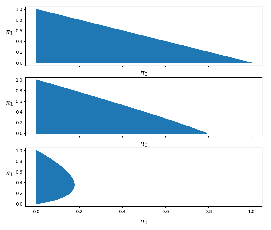
Figure 2: For three offers $a_{0}=90,a_{1}=60,a_{2}=40$ [cf. (6)], this figure shows the values of prior probabilities $\pi_{0}$ and $\pi_{1}$ (depicted by dark domains), where the proposer ${\rm I}$ wins getting smaller regret than the responder ${\rm II}$. From top to bottom: $\beta=1$, $\beta=10$ and $\beta=30$.

V Three (and more) offers

Here we work out (16, 20) and (21–23) for $n\geq 2$, i.e. three or more offers. Define the set $\Omega_{n}$ of winning actions for ${\rm I}$, such that for each $\hat{\pi}\in\Omega_{n}$

$$\Delta R[\hat{a},\hat{p},\hat{\pi}]\equiv R_{{\rm I}}[\hat{a},\hat{p},\hat{\pi}]-R_{{\rm II}}[\hat{a},\hat{p},\hat{\pi}]<0~{}~{}{\rm for~{}any}~{}\hat{p},$$ (43)

where $\hat{p}$ and $\hat{a}$ are defined in (7, 6), respectively. Equivalently, we can define $\Omega_{n}$ via

$${\rm max}_{\hat{p}}\Big{(}\Delta R[\hat{a},\hat{p},\hat{\pi}]\Big{)}<0,$$ (44)

where the maximization in (44) goes over all $\hat{p}$ in (7) for a given $\hat{a}$ in (6). Since $\Delta R[\hat{a},\hat{p},\hat{\pi}]$ in (44) is linear over $\hat{p}$, and the allowed domain (7) of $\hat{p}$ is convex, the maximum in (44) is reached at the end-point of the allowed domain of $\hat{p}$, i.e. we need to check (44) only for non-trivial end-points

$$\hat{p}^{[1]}=(0,1,1,...,1),~{}~{}\hat{p}^{[2]}=(0,0,1,...,1),...,~{}~{}\hat{p}^{[n]}=(0,0,0,...,1).$$ (45)

Hence $\Omega_{n}$ is determined from (44, 45) via simultaneous validity of $n$ inequalities:

$$\Delta R[\hat{a},\hat{p}^{[k]},\hat{\pi}]<0,\quad k=1,...,n.$$ (46)

Fig. 2 reports numerical results for the wining domain (46) of ${\rm I}$ in the three-outcome situation $n=2$. Note that the winning domains of ${\rm I}$ shrink upon increasing $\beta$. The same effect was discussed in section IV.5 for $n=1$ (two offers).

The numerical comparison between scenarios involving two and three offers reveals the following effect of intermediate offers. To illustrate this effect, consider the two-offer situation with $A=100$, $a_{0}=96$, $a_{1}=0$ and $a_{2}=45$ ($\beta=10$ and $u(x)=x$ for concreteness). Here the domain $\Omega_{1}$ of winning actions for ${\rm I}$ is empty, i.e. ${\rm II}$ wins over ${\rm I}$. However, when adding an intermediate offer, i.e. considering $a_{0}=96$, $a_{1}=60$ and $a_{2}=45$ (with the same $\beta=10$ and $A=100$), there emerges a non-empty set $\Omega_{2}$. Likewise, an intermediate offer can improve the maximal mean outcome for ${\rm I}$. For example,

$${\rm max}_{(\pi_{0},\pi_{1},\pi_{2})\in\Omega_{2}}\Big{[}\pi_{0}\times 96+\pi_{1}\times 60+\pi_{2}\times 43\Big{]}=61.01,$$ (47)

$${\rm max}_{(\pi_{0},\pi_{2})\in\Omega_{1}}\Big{[}\pi_{0}\times 96+\pi_{1}\times 0+\pi_{2}\times 43\Big{]}=56.25.$$ (48)

Now ${\rm max}_{(\pi_{0},\pi_{1},\pi_{2})\in\Omega_{2}}\Big{[}\pi_{0}a_{0}+\pi_{1}a_{1}+\pi_{2}a_{2}\Big{]}$ cannot decrease when going from the two-offer situation to the three-offer situation, but there are cases when this quantity does not change upon adding e.g. an intermediate offer. For instance,

$${\rm max}_{(\pi_{0},\pi_{1},\pi_{2})\in\Omega_{2}}\Big{[}\pi_{0}\times 90+\pi_{1}\times 60+\pi_{2}\times 40\Big{]}$$ (49)

$$={{\rm max}}_{{(\pi_{0},\pi_{2})\in\Omega_{1}}}\Big{[}\pi_{0}\times 90+\pi_{1}\times 0+\pi_{2}\times 40\Big{]}=79.5.$$ (50)

Both examples (47, 48) and (49, 50) are possible for the expected utility regret $g[x]\propto x$, as explicitly shown in Appendix B.

There is a sense in which the three-offer ultimatum game approximately reduces to the two-offer situation. We checked numerically that the following relation holds

$${\cal U}_{\rm I}^{[1]}\equiv{\rm max}_{(\pi_{1},\pi_{2})\in\Omega_{1},\,a_{1}}\Big{[}u(a_{1})\pi_{1}+u(a_{2})\pi_{2}\Big{]}$$ (51)

$$\leq {\cal U}_{\rm I}^{[2]}\equiv{\rm max}_{(\pi_{0},\pi_{1},\pi_{2})\in\Omega_{2},\,a_{0}>a_{1}}\Big{[}u(a_{0})\pi_{0}+u(a_{1})\pi_{1}+u(a_{2})\pi_{2}\Big{]}.$$ (52)

Eq. (52) refers to maximization over the winning strategies of ${\rm I}$ in the three offer situation, and simultaneously over the two offers $a_{0}$ and $a_{1}$ [holding $a_{0}>a_{1}$ from (6)]. These are the offers to which ${\rm II}$ need not agree with probability $1$; cf. (7). The rationale of (52) is that $a_{2}$ is fixed, since it is determined by ${\rm II}$ as the offer ${\rm II}$ will accept certainly, while the remaining two offers $a_{0}$ and $a_{1}$ are determined by ${\rm I}$ from maximizing the mean utility. Eq. (51) is the same as (52), but restricted to the two-offer situation. Variables $a_{0}$ and $a_{1}$ in (52) respect $a_{0}>a_{1}>a_{2}$ [cf. (6)], where $a_{2}$ is a fixed parameter. Likewise, variable $a_{1}$ in (51) respect $a_{1}>a_{2}$, where $a_{2}$ is the same parameter as in (52).

The equality in (52) is realized for the expected utility regret $g[x]=x$; see Appendix B. The inequality in (52) means that the three-offer situation is better for ${\rm I}$ than the two-offer situation, i.e. the mini-ultimatum game. However, for realistic choices of parameters, the difference ${\cal U}_{\rm I}^{[2]}-{\cal U}_{\rm I}^{[1]}$ is sufficiently small; see Table 1.

${(\xi,[\pi])}/{(a_{0},a_{1},a_{2},\beta)}$	$(59,51,47,17)$	$(70,54,46,16)$	$(69,55,47,15)$	$(77,61,41,18)$	$(72,56,43,18)$
${\cal U}_{\rm I}^{[1]}$	$53.24$	$55.36$	$54.04$	$62.6$	$59.24$
$(\pi_{0},\pi_{2})$	$(0.52,0.48)$	$(0.39,0.61)$	$(0.32,0.68)$	$(0.6,0.4)$	$(0.56,0.34)$
$\widetilde{{\cal U}}_{\rm I}^{[2]}$	$53.44$	$55.6$	$54.3$	$62.8$	$59.46$
$(\pi_{0},\pi_{1},\pi_{2})$	$(0.39,0.44,0.17)$	$(0.27,0.39,0.34)$	$(0.23,0.28,0.49)$	$(0.55,0.1,0.35)$	$(0.46,0.24,0.3)$

Table 1: Numerical values for quantities defined around (51, 52) for $A=100$. Instead of the maximization given in (52), we defined $\widetilde{{\cal U}}_{\rm I}^{[2]}\equiv{\rm max}_{(\pi_{0},\pi_{1},\pi_{2})\in\Omega_{2},\,a_{1}}\Big{[}u(a_{0})\pi_{0}+u(a_{1})\pi_{1}+u(a_{2})\pi_{2}\Big{]}$ as follows: first we calculate the optimal $a_{2}$ from (51), and then employ it in $\widetilde{{\cal U}}_{\rm I}^{[2]}$, which is optimized over $a_{1}$. For the presented parameter values we get $\widetilde{{\cal U}}_{\rm I}^{[2]}<{{\cal U}}_{\rm I}^{[2]}$, but still $\widetilde{{\cal U}}_{\rm I}^{[2]}\approx{{\cal U}}_{\rm I}^{[2]}$. The third and fifth rows denote the optimal values for (resp.) $(\pi_{0},\pi_{1})$ and $(\pi_{0},\pi_{1},\pi_{2})$ obtained from maximizing that leads to (resp.) ${{\cal U}}_{\rm I}^{[1]}$ and $\widetilde{{\cal U}}_{\rm I}^{[2]}$. It is seen that $\widetilde{{\cal U}}_{\rm I}^{[2]}>{{\cal U}}_{\rm I}^{[1]}$ and $\widetilde{{\cal U}}_{\rm I}^{[2]}\approx{{\cal U}}_{\rm I}^{[1]}$.

VI Summary

The ultimatum game demonstrates a discrepancy between traditional rationality, defined by the subgame perfect Nash equilibrium, and real-world experimental outcomes. Contrary to the classical rational expectations, responders frequently reject sufficiently small offers (compared to the total sum $A$ to be divided), while proposers (possibly anticipating this rejection) do not offer small amounts.

To explain this rejection behavior, we propose a principle: ultimatum offers are more likely to be declined when the responder experiences less regret about rejecting the offer than the proposer would feel for not presenting a more favorable offer. In other words, when the responder is more at ease with the idea of losing the deal, while the proposer would regret deeper for not proposing a better offer, rejections become more likely. Though regret can be applied to quantifying that feeling as well, it is not simply an emotional feeling. It is an objective means of comparing two probabilistic lotteries that holds several crucial principles of rationality and thereby generalizes the expected utility theory that can be also regarded as a limiting form of regret we_regret .

We demonstrate that various observed phenomena in the ultimatum game, typically attributed to fairness, can alternatively be understood through the lens of rational punishment quantified via regret. These include:

1. Fair Division: In the standard concept of fair division, where participants ${\rm I}$ and ${\rm II}$ have equal utility, the initial sum $A$ is divided into two equal halves. Some of our findings align with those derived from fairness-based assumptions, e.g. the responder ${\rm II}$ wins if all offers by the proposer ${\rm I}$ are larger than $A/2$, while viable winning strategies for the proposer ${\rm I}$ exists when at least one offer is smaller than $A/2$.

2. Responses to unfair/fair versus unfair/superfair offers. Our results suggest that ${\rm II}$ rejects the unfair offer more in the unfair/fair scenario than in the unfair/superfair situation. There is no hope of steering ${\rm I}$ toward the superfair option, which explains this effect.

3. Behavior changes with increasing the stakes: we investigated how behavior changes (or remains constant) as both the total sum $A$ and the offer magnitudes increase proportionally. Our explanations are contingent upon whether the utilities for ${\rm I}$ and ${\rm II}$ are identical, revealing distinct predictions when these functions differ. This distinction arises because wealthier participants can tolerate more significant losses and, thus, demand a larger share, contrary to what the fairness theory suggests. This demonstrates a case where considerations of fairness are supplemented by the need to recognize participants’ intentions, particularly in scenarios with varying utility values.

Lastly, we show that when ${\rm I}$ optimizes both offers and strategies to maximize mean utility, the presence of three offers gives no substantial advantages over a simpler mini-ultimatum game with only two offers. Unfortunately, we lack a theoretical argument to explain why this equivalence holds, but extensive numerical testing across diverse parameter values confirms its validity.

To summarize, the regret theory provides a psychologically realistic framework for understanding human decision-making. It considers not only material gains but also the emotional consequences of choices, aligning well with observed human behavior, particularly in situations involving fairness. However, quantifying regret is subjective and varies among individuals, posing a challenge for generalization to e.g. the multiple-respondent ultimatum game hegemon .

Appendix A Alternative theories explaining rejection behavior in the ultimatum game

In addition to the fairness theory reviewed in section I several other explanations were proposed for the rejection behavior in the ultimatum game. According to the anonymity hypothesis, the rejection behavior is caused by players seeking to please (or establish a long-term relationship) with the experimenter bolton_zwick . Proposers wish to show that they are not greedy, hence they do not propose a minimal amount, while responders would like to seem not in need of money, i.e. they reject small offers. The hypothesis posed serious methodological questions that have been met in practice bolton_zwick , i.e. the hypothesis – which assumes that in reality, people would behave according to the classical scenario – has been falsified bolton_zwick . On the other hand, the anonymity hypothesis explains non-trivial outcomes of the dictator game, where the decision of the responder does not have any influence on the outcomes bolton_zwick . The anonymity hypothesis relates to the desire to be perceived as fair, which was also studied in the context of the dictator game fairfair .

Another hypothesis states that the rejection behavior is evolutionary stable given that the ultimatum game is played in populations of agents and holds certain assumptions population . The main of them is that people interchange their roles as proposers and responders, while their behavior as responders is a slow variable population . However, when applied to the basic situation of two players, the scenario of Ref. population leads to an untenable conclusion that the rejection behavior emerges independently of the parameters of the offers.

Yet another explanation of the rejection behavior focused on the role of emotions experienced by responders pillutla . In particular, responders can be envious, which may explain higher rates of rejection of small offers in the ultimatum game georg ; loyola ; kato . Envy occurs when a player cares about not only their own payoff but also about the relative payoff between them and the other player; e.g. the envy model described in georg amounts to choosing a specific utility function that depends on the monetary outcomes of both players. It is important to note, however, that envy is an irrational feeling that cannot be advised from a normative perspective.

Appendix B The expected utility choice for the regret function

For the expected utility choice (24) of the regret function we have

$$R_{{\rm II}}={\rm EU}({\rm II}_{\rm acc})-{\rm EU}({\rm II}_{\rm rej})=\sum_{l=0}^{n}\pi_{l}u(A-a_{l})-\sum_{l=0}^{n}\pi_{l}p_{l}u(A-a_{l}),$$ (53)

$$R_{{\rm II}}=\rho_{{\rm II}}({\rm II}_{\rm acc};{\rm II}_{\rm rej})-\rho_{{\rm II}}({\rm II}_{\rm rej};{\rm II}_{\rm acc})={\rm EU}({\rm II}_{\rm acc})-{\rm EU}({\rm II}_{\rm rej}),$$ (54)

$${\rm EU}({\rm II}_{\rm acc})=\sum_{l=0}^{n}\pi_{l}u(A-a_{l}),\qquad{\rm EU}({\rm II}_{\rm rej})=\sum_{l=0}^{n}\pi_{l}p_{l}u(A-a_{l}),$$ (55)

$$R_{{\rm I}}=\rho_{{\rm I}}({\rm I}_{n};{\rm I}_{0})-\rho_{{\rm I}}({\rm I}_{0};{\rm I}_{n})={\rm EU}({\rm I}_{n})-{\rm EU}({\rm I}_{0}),\qquad{\rm EU}({\rm I}_{n})=u(a_{n}),\qquad{\rm EU}({\rm I}_{0})=\sum_{l=0}^{n}\pi_{l}p_{l}u(a_{l}),$$ (56)

$$R_{{\rm II}}-R_{{\rm I}}=\sum_{l=0}^{n-1}\pi_{l}\Big{[}p_{l}u(a_{l})+(1-p_{l})u(A-a_{l})-u(a_{n})\Big{]}.$$ (57)

Now ${\rm II}$ want to make $R_{{\rm II}}-R_{{\rm I}}$ in (57) possibly small. To this end, ${\rm II}$ chooses:

$$p_{l}=0~{}~{}{\rm for}~{}~{}u(a_{l})>u(A-a_{l})~{}~{}{\rm or}~{}~{}a_{l}>A/2,$$ (58)

$$p_{l}=1~{}~{}{\rm for}~{}~{}u(a_{l})<u(A-a_{l})~{}~{}{\rm or}~{}~{}a_{l}<A/2.$$ (59)

Thus the winning domain $\{\pi_{k}\}_{k=0}^{n}$ of ${\rm I}$ for given $(a_{0}>...>a_{n})$ is determined by putting (58, 59) into (57)

$$R_{{\rm II}}-R_{{\rm I}}=\sum_{a_{l}>A/2}\pi_{l}\Big{[}u(A-a_{l})-u(a_{n})\Big{]}+\sum_{a_{l}<A/2,\,a_{l}\not=a_{n}}\pi_{l}\Big{[}u(a_{l})-u(a_{n})\Big{]}>0.$$ (60)

Let us work out (60) for $n=2$ (three offers). Now winning domains for ${\rm I}$ are found from

$$R_{{\rm II}}-R_{{\rm I}}=\pi_{0}[u(A-a_{0})-u(a_{2})]+\pi_{1}[u(A-a_{1})-u(a_{2})]>0~{}~{}{\rm for}~{}~{}a_{0}>a_{1}>\frac{A}{2}>a_{2},$$ (61)

$$R_{{\rm II}}-R_{{\rm I}}=\pi_{0}[u(A-a_{0})-u(a_{2})]+\pi_{1}[u(a_{1})-u(a_{2})]>0~{}~{}{\rm for}~{}~{}a_{0}>\frac{A}{2}>a_{1}>a_{2}.$$ (62)

In each regime (61) and (62) we set to maximize the mean utility for ${\rm I}$:

$${\cal U}_{\rm I}={\rm max}_{\hat{\pi}}\Big{[}\sum_{k=0}^{2}\pi_{k}u(a_{k})\Big{]}={\rm max}_{\hat{\pi}}\Big{[}\pi_{0}[u(a_{0})-u(a_{2})]+\pi_{1}[u(a_{1})-u(a_{2})]\Big{]}+u(a_{2}),$$ (63)

where the maximization is carried out over $(\pi_{0},\pi_{1})$ that hold (61) or (62).

Within the regime (61) we are back to the two-offer situation, i.e. for $u(A-a_{0})>u(a_{2})$ (or $a_{0}+a_{2}<A$) the maximization in (63) produces $\pi_{0}=1$, while for $u(A-a_{0})<u(a_{2})g$, (61) is invalid, i.e. ${\rm II}$ wins. Now for (62) the maximization in (63) is reached at the border, i.e. for $R_{{\rm II}}-R_{{\rm I}}\to 0+$ and leads to

$${\cal U}_{\rm I}=\pi_{c}[u(a_{0})-u(a_{2})]+(1-\pi_{c})[u(a_{1})-u(a_{2})]+u(a_{2}),\qquad\pi_{c}=1-{\rm Max}\Big{[}0,\frac{u(a_{2})-u(A-a_{0})}{u(a_{1})-u(A-a_{0})}\Big{]}.$$ (64)

The non-trivial fact about (64) is that for $u(A-a_{0})\geq u(a_{2})$ the action of ${\rm I}$ is probabilistic and amounts to offering $A-a_{0}$ and $A-a_{1}$ with probabilities $\pi_{c}$ and $1-\pi_{c}$, respectively. The meaning of this probabilistic action was already discussed in the main text: from the two-offer viewpoint the regime $u(A-a_{0})<u(a_{2})$ makes ${\rm II}$ to win over ${\rm I}$, and then employing the intermediate offer $a_{1}$ (for the present case it should hold $a_{1}<A/2$, as (62) shows) leads to ${\rm I}$ winning over ${\rm II}$.

We checked that if (64) is maximized (in its validity regime, i.e. for $a_{1}<A/2$ and $a_{0}+a_{2}>A$) over $a_{0}$, then the maximum of ${\cal U}_{\rm I}$ is reached for $a_{0}+a_{2}\to A$, i.e. for $\pi_{c}\to 1$. In that sense, we are effectively back to the two-offer situation.

Appendix C Transitive regret

The intuitive meaning of (26) is explained as follows we_regret : the exponential form $f[x]\propto e^{\beta x}$ is the only one that holds the multiplicativity feature $f[x+y]=f[x]f[y]$ that produces (26) via (19). For certain applications, the transitivity can be lifted and more general forms of $f[x]$ can be employed we_regret , but we do not focus on such forms here. Eq. (26) shows that we are back from the regret theory to the expected utility theory for $\beta\to\infty$; cf. (24).

We note that $g[x]$ in (26) holds the following two features that make a general sense in the intuitive context of regret:

$$g[x+y]>g[x]+g[y],\qquad x>0,~{}~{}y>0,$$ (65)

$$g[x-y]\leq g[x]-g[y],\qquad x>y>0,$$ (66)

where (66) is deduced in (31), and (65) is derived along the same lines. Eqs. (65, 66) make intuitive sense. According to (65), regret tends to be larger when the regret-inducing stimulus is presented in total $x+y$ rather than in separate $x$ and $y$ pieces. Likewise, (66) means that the regret is larger when two stimuli of different signs are arranged in parallel, as compared to the total, smaller, and positive stimulus $x-y$.

References

- (1) W. Güth, R. Schmittberger, and B. Schwarze, “An experimental analysis of ultimatum bargaining,” Journal of economic behavior & organization, vol. 3, no. 4, pp. 367–388, 1982.
- (2) S. J. Solnick, “Gender differences in the ultimatum game,” Economic Inquiry, vol. 39, no. 2, pp. 189–200, 2001.
- (3) S. J. Solnick and M. E. Schweitzer, “The influence of physical attractiveness and gender on ultimatum game decisions,” Organizational behavior and human decision processes, vol. 79, no. 3, pp. 199–215, 1999.
- (4) H. Oosterbeek, R. Sloof, and G. Van De Kuilen, “Cultural differences in ultimatum game experiments: Evidence from a meta-analysis,” Experimental economics, vol. 7, pp. 171–188, 2004.
- (5) S.-H. Chuah, R. Hoffmann, M. Jones, and G. Williams, “Do cultures clash? evidence from cross-national ultimatum game experiments,” Journal of Economic Behavior & Organization, vol. 64, no. 1, pp. 35–48, 2007.
- (6) ——, “An economic anatomy of culture: Attitudes and behaviour in inter-and intra-national ultimatum game experiments,” Journal of Economic Psychology, vol. 30, no. 5, pp. 732–744, 2009.
- (7) D. G. Rand, C. E. Tarnita, H. Ohtsuki, and M. A. Nowak, “Evolution of fairness in the one-shot anonymous ultimatum game,” Proceedings of the National Academy of Sciences, vol. 110, no. 7, pp. 2581–2586, 2013.
- (8) B. J. Ruffle, “More is better, but fair is fair: Tipping in dictator and ultimatum games,” Games and Economic Behavior, vol. 23, no. 2, pp. 247–265, 1998.
- (9) P. G. Straub and J. K. Murnighan, “An experimental investigation of ultimatum games: Information, fairness, expectations, and lowest acceptable offers,” Journal of Economic Behavior & Organization, vol. 27, no. 3, pp. 345–364, 1995.
- (10) E. Fehr and K. M. Schmidt, “A theory of fairness, competition, and cooperation,” The quarterly journal of economics, vol. 114, no. 3, pp. 817–868, 1999.
- (11) W. Güth, S. Huck, and W. Müller, “The relevance of equal splits in ultimatum games,” Games and Economic Behavior, vol. 37, no. 1, pp. 161–169, 2001.
- (12) T. Yamagishi, Y. Horita, N. Mifune, H. Hashimoto, Y. Li, M. Shinada, A. Miura, K. Inukai, H. Takagishi, and D. Simunovic, “Rejection of unfair offers in the ultimatum game is no evidence of strong reciprocity,” Proceedings of the National Academy of Sciences, vol. 109, no. 50, pp. 20 364–20 368, 2012.
- (13) L. J. Savage, “The theory of statistical decision,” Journal of the American Statistical association, vol. 46, no. 253, pp. 55–67, 1951.
- (14) D. E. Bell, “Regret in decision making under uncertainty,” Operations research, vol. 30, no. 5, pp. 961–981, 1982.
- (15) G. Loomes and R. Sugden, “Regret theory: An alternative theory of rational choice under uncertainty,” The economic journal, vol. 92, no. 368, pp. 805–824, 1982.
- (16) V. G. Bardakhchyan and A. E. Allahverdyan, “Regret theory, allais’ paradox, and savage’s omelet,” arXiv preprint arXiv:2301.02447, 2023.
- (17) A. Falk, E. Fehr, and U. Fischbacher, “On the nature of fair behavior,” Economic inquiry, vol. 41, no. 1, pp. 20–26, 2003.
- (18) G. E. Bolton and R. Zwick, “Anonymity versus punishment in ultimatum bargaining,” Games and Economic behavior, vol. 10, no. 1, pp. 95–121, 1995.
- (19) S. Huck and J. Oechssler, “The indirect evolutionary approach to explaining fair allocations,” Games and economic behavior, vol. 28, no. 1, pp. 13–24, 1999.
- (20) J. Gale, K. G. Binmore, and L. Samuelson, “Learning to be imperfect: The ultimatum game,” Games and economic behavior, vol. 8, no. 1, pp. 56–90, 1995.
- (21) R. B. Myerson, Game theory: analysis of conflict. Harvard university press, 1991.
- (22) E. Hoffman, K. A. McCabe, and V. L. Smith, “On expectations and the monetary stakes in ultimatum games,” International Journal of Game Theory, vol. 25, no. 3, pp. 289–301, 1996.
- (23) K. Telser, “The ultimatum game: A comment,” Mimeo, Department of Economics, University of Chicago, Tech. Rep., 1993.
- (24) R. E. Goodin, “How amoral is hegemon?” Perspectives on Politics, vol. 1, no. 1, pp. 123–126, 2003.
- (25) J. Andreoni and B. D. Bernheim, “Social image and the 50–50 norm: A theoretical and experimental analysis of audience effects,” Econometrica, vol. 77, no. 5, pp. 1607–1636, 2009.
- (26) M. M. Pillutla and J. K. Murnighan, “Unfairness, anger, and spite: Emotional rejections of ultimatum offers,” Organizational behavior and human decision processes, vol. 68, no. 3, pp. 208–224, 1996.
- (27) G. Kirchsteiger, “The role of envy in ultimatum games,” Journal of economic behavior & organization, vol. 25, no. 3, pp. 373–389, 1994.
- (28) G. Loyola, “Alternative equilibria in two-period ultimatum bargaining with envy,” Optimization Letters, vol. 11, pp. 855–874, 2017.
- (29) H. Takahashi, M. Kato, M. Matsuura, D. Mobbs, T. Suhara, and Y. Okubo, “When your gain is my pain and your pain is my gain: neural correlates of envy and schadenfreude,” Science, vol. 323, no. 5916, pp. 937–939, 2009.