Ensembling Textual and Structure-Based Models for
Knowledge Graph Completion

Abstract

We consider two popular approaches to Knowledge Graph Completion (KGC): textual models that rely on textual entity descriptions, and structure-based models that exploit the connectivity structure of the Knowledge Graph (KG). Preliminary experiments show that these approaches have complementary strengths: structure-based models perform well when the gold answer is easily reachable from the query head in the KG, while textual models exploit descriptions to give good performance even when the gold answer is not reachable. In response, we explore ensembling as a way of combining the best of both approaches. We propose a novel method for learning query-dependent ensemble weights by using the distributions of scores assigned by individual models to all candidate entities. Our ensemble baseline achieves state-of-the-art results on three standard KGC datasets, with up to 6.8 pt MRR and 8.3 pt Hits@1 gains over best individual models.

1 Introduction

The task of Knowledge Graph Completion (KGC) can be described as inferring missing links in a Knowledge Graph (KG) based on given triples ($\fol{h},\fol{r},\fol{t}$), where $\fol{r}$ is a relation that exists between the head entity $\fol{h}$ and the tail entity $\fol{t}$. Several KGC approaches, such as NBFNet Zhu et al. (2021) and RGHAT Zhang et al. (2020), exploit the underlying graph structure, often using GNNs. On the other hand, textual models such as SimKGC Wang et al. (2022) and KG-BERT Yao et al. (2019) leverage pre-trained large language models (LLMs) such as BERT to utilize textual descriptions of the KG entities and relations for KGC.

Our preliminary experiments suggest that when the gold answer $\fol{t}$ for query ($\fol{h},\fol{r},?$) is reachable from $\fol{h}$ using a path of reasonable length in the KG, structure-based models tend to outperform textual models. In contrast, textual models can use textual descriptions to perform better than structure-based models when $\fol{t}$ is not easily reachable from $\fol{h}$. Motivated by our findings, we seek to explore how ensembling, an approach currently underrepresented in KGC literature, can effectively harness the complementary strengths of these models.

Consequently, we develop a new strong baseline for KGC by ensembling two strong KGC models: SimKGC and NBFNet, which are textual and structure-based in nature, respectively. We also propose a novel, simple, model-agnostic and lightweight method for learning ensemble weights such that the weights are (i) query-dependent and (ii) learned from statistical features obtained from the distribution of scores assigned by individual models to all candidate entities.

On three KGC datasets, we find that applying our ensembling method to SimKGC and NBFNet consistently improves KGC performance, outperforming best individual models by up to 6.8 pt MRR and 8.3 pt Hits@1. To the best of our knowledge, these results are state-of-the-art for all three datasets. Further experiments (including a fourth dataset to which NBFNet does not scale) show that our approach generalises to ensembling with another KG embedding model, RotatE Sun et al. (2019), with similar gains. We also demonstrate that our ensemble learning methodology outperforms conventional model-combination techniques such as static ensembling (where the ensemble weight is a tuned constant hyperparameter) and re-ranking. We release all code to guide future research.

2 Background and Related Work

Task: We are given an incomplete KG $\mathcal{K}=(\mathcal{E},\mathcal{R},\mathcal{T})$ consisting of entities $\mathcal{E}$, relation set $\mathcal{R}$ and set of triples $\mathcal{T}=\{(\fol{h},\fol{r},\fol{t})\}$ (where $\fol{h},\fol{t}\in\mathcal{E}$ and $\fol{r}\in\mathcal{R}$). The goal of KGC is to answer queries of the form $(\fol{h},\fol{r},?)$ or $(?,\fol{r},\fol{t})$ to predict missing links, with corresponding answers $\fol{t}$ and $\fol{h}$. We model $(?,\fol{r},\fol{t})$ as $(\fol{t},\fol{r^{-1}},?)$ queries in this work.

Overview of Related Work: We focus on three types of KGC models. The first type consists of Graph Neural Network (GNN) based models such as NBFNet Zhu et al. (2021), RGHAT Zhang et al. (2020) that leverage neighborhood information to train distinct GNN architectures. The second type contains textual models such as KG-BERT Yao et al. (2019) and SimKGC Wang et al. (2022) which exploit textual descriptions of entities and relations to fine-tune a pre-trained LLM for KGC. The third type involves models such as RotatE Sun et al. (2019) and TransE Bordes et al. (2013) that learn low-dimensional embeddings for entities and relations and compose them by employing unique scoring functions. Ensembling of these models has not been extensively studied before in KGC literature, although models such as RNNLogic Qu et al. (2021) have used static ensembling with KG embedding models like RotatE to improve performance. Since our main experiments are based on NBFNet, SimKGC and RotatE, we describe these in some detail next.

NBFNet: Neural Bellman-Ford Network (NBFNet) is a path-based link prediction model that introduces neural functions into the Generalized Bellman-Ford (GBF) Algorithm Baras and Theodorakopoulos (2010), which in turn models the path between two nodes in the KG through generalized sum and product operators. This formulates a novel GNN framework that learns entity representations for each candidate tail $\fol{t}$ conditioned on $\fol{h}$ and $\fol{r}$ for each query $(\fol{h},\fol{r},?)$. The score of any candidate $\fol{t}$ is then computed by applying an MLP to its embedding.

SimKGC: SimKGC is an LLM-based KGC model that employs a bi-encoder architecture to generate the score of a given triple ($\fol{h},\fol{r},\fol{t}$). The model considers two pre-trained BERT Devlin et al. (2019) models. The first model is finetuned on a concatenation of textual descriptions of $\fol{h}$ and $\fol{r}$ to generate their joint embedding $\textbf{e}_{hr}$ and the second model is finetuned on the textual description of $\fol{t}$ to generate the embedding $\textbf{e}_{t}$. The score for the triple is the cosine similarity between $\textbf{e}_{hr}$ and $\textbf{e}_{t}$.

RotatE: RotatE is a KG Embedding model that maps entities and relations to a complex vector space and models each relation $\fol{r}$ as a complex rotation from the head $\fol{r}$ to the tail $\fol{t}$ for triple ($\fol{h},\fol{r},\fol{t}$). More specifically, the scoring function of RotatE is $\left\|\textbf{h}\circ\textbf{r}-\textbf{t}\right\|$ where $\textbf{h},\textbf{t}\in\mathbb{C}^{k}$ are the complex embedding of $\fol{h}$ and $\fol{t}$, and $\circ$ is the Hadamard product.

3 Ensemble Methodology

Our goal is to effectively ensemble $k$ KGC models $\fol{M_{i}}$, which may be textual or structure-based, to improve overall performance. Each model $\fol{M_{i}}$ assigns a score $\fol{M_{i}(h,r,t)}$ to all candidate tails $\fol{t}\in\mathcal{E}$ for query $\fol{q}=(\fol{h},\fol{r},?)$. These models are trained independently and their parameters are frozen before ensembling. We formulate the ensemble $\fol{E}$ as:

$$\fol{E(h,r,t)}=\sum_{i=1}^{k}\fol{w_{i}(q)M_{i}(h,r,t)}$$

where $\fol{E(h,r,t)}$ is the ensemble score for $\fol{t}$ given query $\fol{q}=\fol{(h,r,?)}$. Since $\fol{M_{i}(h,r,t)}$ typically lies in differing ranges for each model $\fol{M_{i}}$, we first normalize these scores as described below.

Normalization: To bring the distribution of scores assigned by each model $\fol{M_{i}}$ over all $\fol{t}\in\mathcal{E}$ in the same range for each query, we max-min normalize the scores obtained from all models $\fol{M_{i}}$ separately:

$$\vspace{-0.05in}\fol{M_{i}(h,r,t)}\leftarrow\fol{M_{i}(h,r,t)}-\min_{\fol{t^{\prime}}\in\,\mathcal{E}}{\fol{M_{i}(h,r,t^{\prime})}}\vspace{-0.02in}$$

$$\vspace{-0.05in}\fol{M_{i}(h,r,t)}\leftarrow\frac{\fol{M_{i}(h,r,t)}}{\max_{t^{\prime}\in\mathcal{E}}{\fol{M_{i}(h,r,t^{\prime})}}}$$

The scores obtained after normalization always lie in the range [0,1] for all models. We next describe the simple model used to learn the query-dependent ensemble weights $\fol{w_{i}}$.

Table 1: Results on four datasets for our baselines and approach. $\fol{[NBF]}$, $\fol{[Sim]}$ and $\fol{[RotE]}$ represent $\fol{NBFNet}$, $\fol{SimKGC}$ and $\fol{RotatE}$ models. $\fol{[NBF]}$ does not scale up to YAGO3-10. Best individual model results are underlined.

Model	WN18RR			FB15k-237			CoDex-M			YAGO3-10
	MRR	H@1	H@10	MRR	H@1	H@10	MRR	H@1	H@10	MRR	H@1	H@10
$\fol{[Sim]}$	66.4	58.5	80.3	32.1	23.2	50.5	29.1	21.0	45.2	15.8	10.0	27.3
$\fol{[NBF]}$	54.2	48.6	65.7	40.5	31.0	59.4	35.3	27.0	51.4	-	-	-
$\fol{[RotE]}$	47.7	43.9	55.2	33.7	24.0	53.2	33.5	26.3	46.9	49.3	39.9	67.1
$\fol{[Sim]}$+$\fol{[NBF]}$	73.2	66.9	85.7	42.7	33.2	61.5	38.9	30.5	54.8	-	-	-
$\fol{[Sim]}$+$\fol{[RotE]}$	68.0	60.7	80.7	36.6	26.9	56.3	36.3	28.1	51.7	50.6	41.3	67.9
$\fol{[Sim]}$+$\fol{[NBF]}$+$\fol{[RotE]}$	73.2	66.9	85.7	43.0	33.4	62.0	40.0	31.2	54.8	-	-	-

Model: We extract the following features from the score distribution of each model $\fol{M_{i}}$:

$$\fol{f(M_{i},q)}=\fol{\operatorname*{mean}_{t^{\prime}\in\mathcal{E}}({M_{i}(h,r,t^{\prime})})}||\fol{\operatorname*{var}_{t^{\prime}\in\mathcal{E}}({M_{i}(h,r,t^{\prime})})}$$

In the above equations, $\operatorname*{mean}()$ and $\operatorname*{var}()$ are the standard mean and variance functions respectively, whose outputs are concatenated to obtain the feature. This choice is motivated by our observation that the variance and mean of the distribution of scores computed by any model over $\mathcal{E}$ is correlated to its confidence about its top predictions. A more detailed discussion can be found in Appendix C.

Next, we concatenate these features for all $\fol{M_{i}}$ to obtain a final feature vector that is passed to an independent 2-layer MLP ($\fol{MLP_{i}}$) for each model $\fol{M_{i}}$ to learn query-dependent $\fol{w_{i}}$:

$$\fol{w_{i}(q)}=\fol{MLP_{i}}(\fol{f(M_{1},q)||f(M_{2},q)||...||f(M_{k},q)})$$

Intuitively, concatenating these features over all models informs each MLP about the relative confidence of all models regarding their predictions, enhancing the ensemble weight computation for corresponding models. Note that our approach is agnostic to specific models $\fol{M_{i}}$.

Our experiments in this paper involve only one textual model. Therefore, we learn the ensemble weights for the other models with respect to this textual model, which is assigned a fixed weight of 1. This decreases the parameter count while also being as expressive as learning distinct ensemble weights for all models. The method for learning these other weights is unchanged.

Loss Function: We train our model on the validation set (traditionally used to tune ensemble weights) using margin loss between the score of the gold entity and a set of negative samples. The train set is not used since all models are likely to give high-confidence predictions on its triples. If the gold entity is $\fol{t^{*}}$ and the set of negative samples is $\fol{N}$, the loss function $\mathcal{L}$ for query $\fol{q}=\fol{(h,r,?)}$ is:

$$\mathcal{L}=\sum_{\fol{t}\in\fol{N}}{\max{\fol{(E(h,r,t)-E(h,r,t^{*})+m,0)}}}$$

where $\fol{m}$ is the margin hyperparameter.

4 Experiments

Datasets: We use four datasets for evaluation: WN18RR Dettmers et al. (2018), FB15k-237 Toutanova and Chen (2015), CoDex-M Safavi and Koutra (2020) and YAGO3-10 Mahdisoltani et al. (2015). For each triple in the test set, we answer queries $\fol{(h,r,?)}$ and $\fol{(t,r^{-1},?)}$ with answers $\fol{t}$ and $\fol{h}$. We report the Mean Reciprocal Rank (MRR) and Hits@k (H@1, H@10) under the filtered measures Bordes et al. (2013). Details and data statistics are in Appendix A.

Baselines: We use $\fol{SimKGC}$ ($\fol{[Sim]}$ in tables) as a state of the art textual model baseline. $\fol{NBFNet}$ ($\fol{[NBF]}$ in tables) serves as a strong structure-based model baseline. We also present results with $\fol{RotatE}$ ($\fol{[RotE]}$ in tables) to showcase the generalisation of our method to KG embedding models. We have reproduced the numbers published by the original authors for these baselines. Since $\fol{[NBF]}$ does not scale up to YAGO3-10 with reasonable hyperparameters on our hardware, we omit those results. We represent ensembling by $\fol{+}$ in tables.

Experimental Setup: All baseline models are frozen after training using optimal configurations. Ensemble weights are trained on the validation split, using Adam as the optimizer with a learning rate of 5.0e-5. We use 10,000 negative samples per query. MLP hidden dimensions are set to 16 and 32 for ensemble of 2 and 3 models respectively. MLP weights are initialized uniformly in the range [0, 2]. Training of the ensemble converges in a single epoch, making our method fast and efficient.

Results: We report the results of ensembling in Table 1 (more details in Appendix B). We observe a notable increase in performance after ensembling with $\fol{[Sim]}$ for both $\fol{[NBF]}$ and $\fol{[RotE]}$, which shows that our approach works with both structure-based and KG embedding models. In particular, we obtain 6.8 pt MRR and 8.4 pt Hits@1 improvement with $\fol{[Sim]}+\fol{[NBF]}$ over $\fol{[Sim]}$ on WN18RR. Ensembling with $\fol{[Sim]}$ results in substantial performance gains even when it is outperformed by the other models (on FB15k-237, CoDex-M and YAGO3-10). Notably, on YAGO3-10, where $\fol{[RotE]}$ outperforms $\fol{[Sim]}$ by 33.5 pt MRR and 29.9 pt Hits@1, we still obtain 1.3 pt MRR and 1.4 pt Hits@1 gain with $\fol{[Sim]}$ + $\fol{[RotE]}$ over $\fol{[RotE]}$. Results for $\fol{[Sim]}+\fol{[NBF]}$ + $\fol{[RotE]}$ show that ensembling with $\fol{[RotE]}$ results in marginal gains over $\fol{[Sim]}+\fol{[NBF]}$, obtaining up to 1.1 pt MRR and 0.7 pt Hits@1 gain on CoDex-M. We hypothesize that the gains are marginal due to $\fol{[RotE]}$’s ability to capture some structural information (explored in more detail in Appendix D and E) and drawing inferences based on it, making it somewhat redundant in the presence of $\fol{[NBF]}$. To the best of our knowledge, our best results on WN18RR, FB15k-237 and CoDex-M datasets are state of the art.

5 Analysis

We perform three further analyses to answer the following questions: Q1. How does the behavior of textual and structure-based models vary with reachability? Q2. Do the weights learned by our approach follow expected trends with reachability? Q3. Does our approach improve performance over conventional model-combination techniques?

Reachability Ablation: To answer Q1, we divide the test set for each dataset into ‘reachable’ and ‘unreachable’ splits. A triple $\fol{(h,r,t)}$ is part of the reachable split if $\fol{t}$ can be reached from $\fol{h}$ with a path of length at most $\fol{l}$ (= 2) in the KG. If not, it is put in the unreachable split. We present split-wise results for $\fol{[NBF]}$, $\fol{[Sim]}$ and $\fol{[Sim]}$+$\fol{[NBF]}$ on the WN18RR and FB15k-237 datasets in Table 2.

Table 2: Results on Reachable and Unreachable Split of $\fol{[NBF]}$, $\fol{[Sim]}$ and $\fol{[NBF]}$ + $\fol{[Sim]}$ on WN18RR and FB15k-237. Best individual model results are underlined.

Dataset	Model	Reachable Split			Unreachable Split
		MRR	H@1	H@10	MRR	H@1	H@10
WN18RR	$\fol{[NBF]}$	89.7	86.8	95.7	26.0	18.3	41.8
	$\fol{[Sim]}$	85.3	79.4	94.5	51.8	42.3	69.0
	$\fol{[Sim]}$+$\fol{[NBF]}$	93.9	91.7	97.4	56.8	47.0	76.4
FB15k$-$237	$\fol{[NBF]}$	44.8	35.2	64.0	28.2	19.3	46.2
	$\fol{[Sim]}$	31.5	22.6	49.6	30.0	21.2	48.2
	$\fol{[Sim]}$+$\fol{[NBF]}$	46.5	36.8	65.3	32.3	23.1	50.6

We observe that $\fol{[Sim]}$ outperforms $\fol{[NBF]}$ on the unreachable split (by up to 25.8 pt MRR and 24.0 pt Hits@1 for WN18RR), while $\fol{[NBF]}$ outperforms $\fol{[Sim]}$ on the reachable split (by up to 13.3 pt MRR and 12.6 pt Hits@1 for FB15k-237). This is because $\fol{[NBF]}$ can exploit knowledge of the KG structure when the gold entity $\fol{t}$ is easily reachable from query head $\fol{h}$, while $\fol{[Sim]}$ can instead use BERT to leverage textual descriptions when no such path is present. The performance gap between $\fol{[Sim]}$ and $\fol{[NBF]}$ on the unreachable split is notably larger for WN18RR than for FB15k-237, which can be attributed to the sparsity of the WN18RR dataset, which also has several unseen entities in this split. In such cases, $\fol{[Sim]}$ leverages textual descriptions to achieve reasonable performance, whereas $\fol{[NBF]}$ lacks any paths for reasoning. Our ensemble obtains substantial gains over best individual models on both splits, with 4.2 pt MRR and 4.9 pt Hits@1 gain on the reachable split and 5.0 pt MRR and 4.7 pt Hits@1 gain on the unreachable split for WN18RR. More details in Appendix D.

Analysis of Ensemble Weights: To answer Q2, we study the mean of the ensemble weight $\fol{w_{2}}$ for $\fol{[Sim]}$ + $\fol{[NBF]}$ over the queries in the reachable and unreachable splits of the datasets we use. We observe that this mean is consistently larger (by a margin of up to 17% for WN18RR) on the reachable split than the unreachable split. This is because $\fol{[NBF]}$ tends to give better performance on the reachable split, and a larger $\fol{w_{2}}$ gives it more importance in the ensemble. More details and numbers are in Appendix F, which also shows the non-trivial standard deviation of $\fol{w_{2}}$, demonstrating our approach’s ability to adjust it as required by individual queries.

Comparison with Conventional Techniques: To answer Q3, we present results for static ensembling and re-ranking using $\fol{[Sim]}$ and $\fol{[NBF]}$ for WN18RR and FB15k-237 datasets in Table 3. ‘Static ensembling’ involves tuning the ensemble weight as a constant on the validation set. We call our ensembling approach ‘dynamic ensembling’. For $\fol{[NBF]}$-$\fol{[Sim]}$ re-ranking Han et al. (2020), we consider the top 100 entities by score from $\fol{[NBF]}$ for each query and rank them according to their $\fol{[Sim]}$ score. The rest of the entities are ranked according to $\fol{[NBF]}$. We also present results for $\fol{[Sim]}$-$\fol{[NBF]}$ re-ranking.

Table 3: Comparison of Static and Dynamic Ensembling and Re-ranking. $\fol{[X]}$-$\fol{[Y]}$ re-ranking indicates re-ranking of top 100 predictions from $\fol{[X]}$ using $\fol{[Y]}$.

Dataset	Approach	MRR	H@1	H@10
WN18RR	$\fol{[NBF]}$-$\fol{[Sim]}$ Re-rank	63.5	57.1	74.9
	$\fol{[Sim]}$-$\fol{[NBF]}$ Re-rank	60.7	53.3	76.0
	Static Ensemble	72.2	65.5	85.4
	Dynamic Ensemble	73.2	66.9	85.7
FB15k$-$237	$\fol{[NBF]}$-$\fol{[Sim]}$ Re-rank	32.7	23.3	52.5
	$\fol{[Sim]}$-$\fol{[NBF]}$ Re-rank	38.9	30.0	56.5
	Static Ensemble	41.9	32.7	60.1
	Dynamic Ensemble	42.7	33.2	61.5

We find that our ‘dynamic ensemble’ approach outperforms both re-ranking and ‘static ensembling’ across datasets. Notably, our approach beats re-ranking by 9.7 pt MRR and 9.8 pt Hits@1, and static ensembling by 1.0 pt MRR and 1.4 pt Hits@1 on the WN18RR dataset. This highlights the utility of our simple ensemble learning approach.

6 Conclusion and Future Work

We present a simple, novel, model-agnostic and lightweight ensembling approach for the task of KGC, while also highlighting the complementary strengths of textual and structure-based KGC models. Our state-of-the-art results for $\fol{[Sim]}$ + $\fol{[NBF]}$ over three standard KGC datasets creates a new competitive ensemble baseline for future KGC. We release all code for future research. Future work includes better and tighter unification methods for textual and structure-based KGC.

Limitations

We do not consider Neuro-Symbolic KGC approaches in this work, which have also recently started to give competitive results with other KGC approaches, through models such as RNNLogic Qu et al. (2021). Our experiments consider ensembling of one textual model with multiple structural models. This is because most textual models in recent KGC literature are not competitive with SimKGC Wang et al. (2022). The ensembling of multiple textual models with multiple structure-based models would be a possible future work. In models with substantial validation splits, learning query embeddings to augment the features we use to compute ensemble weights is also a possibility.

Ethics Statement

We anticipate no substantial ethical issues arising due to our work on ensembling textual and structure-based models for KGC. Our work relies on other baseline models for ensembling. This may propagate any bias present in these baseline models, however ensembling may also reduce these biases.

Table 4: Statistics of Knowledge Graph datasets

Datasets	#Entities	#Relations	#Training	#Validation	#Test
FB15k-237	14541	237	272,115	17,535	20,446
WN18RR	40,943	11	86,835	3,034	3,134
Yago3-10	123182	36	1,079,040	5000	5000
CoDex-M	17050	71	185584	10310	10311

Table 5: Results of on four datasets: WN18RR, FB15k-237, Yago3-10 and CoDex-M with ensemble of textual and structure-based models. $\fol{[NBF]}$, $\fol{[Sim]}$, $\fol{[RotE]}$ and $\fol{[Comp]}$ represents NBFNet, SimKGC, RotatE and CompleX models respectively. $\fol{[NBF]}$ does not scale to YAGO3-10. Best individual model results are underlined.

Model	WN18RR					FB15k-237
	MR	MRR	H@1	H@3	H@10	MR	MRR	H@1	H@3	H@10
$\fol{[Sim]}$	174.0	66.4	58.5	71.3	80.3	131.9	32.1	23.2	34.6	50.5
$\fol{[NBF]}$	699.3	54.2	48.6	56.9	65.7	111.4	40.5	31.0	44.3	59.4
$\fol{[RotE]}$	4730.7	47.7	43.9	49.1	55.2	176.6	33.7	24.0	37.4	53.2
$\fol{[Comp]}$	5102.6	47.2	42.8	49.2	56.0	180.7	35.7	26.3	39.4	54.7
$\fol{[Sim]}$+$\fol{[NBF]}$	56.6	73.2	66.9	76.5	85.7	92.2	42.7	33.2	46.7	61.5
$\fol{[Sim]}$+$\fol{[RotE]}$	162.7	68.0	60.7	72.2	80.7	116.0	36.6	26.9	40.2	56.3
$\fol{[Sim]}$+$\fol{[Comp]}$	172.9	68.0	60.8	72.3	80.7	116.3	37.8	28.3	41.2	57.1
$\fol{[Sim]}$+$\fol{[NBF]}$+$\fol{[RotE]}$	56.6	73.2	66.9	76.5	85.7	91.5	43.0	33.4	47.0	62.0
$\fol{[Sim]}$+$\fol{[NBF]}$+$\fol{[Comp]}$	56.6	73.2	66.9	76.5	85.7	92.0	42.8	33.3	46.8	61.5
Model	CoDex-M					Yago3-10
	MR	MRR	H@1	H@3	H@10	MR	MRR	H@1	H@3	H@10
$\fol{[Sim]}$	284.2	29.1	21.0	31.5	45.2	497.4	15.8	10.0	16.2	27.3
$\fol{[NBF]}$	337.5	35.3	27.0	39.0	51.4	-	-	-	-	-
$\fol{[RotE]}$	502.6	33.5	26.3	36.8	46.9	1866.8	49.3	39.9	55.0	67.1
$\fol{[Comp]}$	391.0	35.3	27.7	38.8	49.5	1578.1	49.2	40.1	53.8	66.7
$\fol{[Sim]}$+$\fol{[NBF]}$	252.1	38.9	30.5	42.7	54.8	-	-	-	-	-
$\fol{[Sim]}$+$\fol{[RotE]}$	293.4	36.3	28.1	40.0	51.7	610.6	50.6	41.3	56.0	67.9
$\fol{[Sim]}$+$\fol{[Comp]}$	296.3	37.5	29.6	41.0	52.4	515.9	49.5	40.5	54.2	66.6
$\fol{[Sim]}$+$\fol{[NBF]}$+$\fol{[RotE]}$	216.5	40.0	31.2	43.3	54.8	-	-	-	-	-
$\fol{[Sim]}$+$\fol{[NBF]}$+$\fol{[Comp]}$	293.3	37.6	29.8	41.1	52.5	-	-	-	-	-

Table 6: Results of $\fol{[Sim]}$, $\fol{[NBF]}$, $\fol{[RotE]}$, $\fol{[Comp]}$ and $\fol{[Sim]}$ + $\fol{[NBF]}$ on the Reachable and Unreachable splits of WN18RR, FB15k-237, and CoDex-M datasets. Best individual model results are underlined.

Dataset	Model	Reachable Split				Unreachable Split
		MR	MRR	H@1	H@10	MR	MRR	H@1	H@10
WN18RR	$\fol{[Sim]}$	29.7	85.3	79.4	94.5	288.5	51.8	42.3	69.0
	$\fol{[NBF]}$	4.7	89.7	86.8	95.7	1250.7	26.0	18.3	41.8
	$\fol{[RotE]}$	102.9	85.6	83.3	90.0	8404.8	17.5	12.6	1.1
	$\fol{[Comp]}$	285.9	85.6	83.8	88.5	10526.6	16.2	12.1	23.7
	$\fol{[Sim]}$+$\fol{[NBF]}$	2.7	93.9	91.7	97.4	99.4	56.8	47.0	76.4
FB15k$-$237	$\fol{[Sim]}$	131.8	31.5	22.6	49.6	153.8	30.0	21.2	48.2
	$\fol{[NBF]}$	86.9	44.8	35.2	64.0	180.4	28.2	19.3	46.2
	$\fol{[RotE]}$	131.8	35.6	25.5	56.3	303.2	28.1	19.8	44.5
	$\fol{[Comp]}$	129.9	37.9	28.0	57.8	323.9	29.7	21.5	46.0
	$\fol{[Sim]}$+$\fol{[NBF]}$	76.0	46.5	36.8	65.3	137.0	32.3	23.1	50.6
CoDex$-$M	$\fol{[Sim]}$	166.5	35.5	26.8	52.4	363.6	23.7	15.8	39.6
	$\fol{[NBF]}$	150.1	47.8	39.5	63.2	458.1	27.2	18.9	43.5
	$\fol{[RotE]}$	290.5	44.2	37.2	56.8	639.1	26.7	19.5	40.5
	$\fol{[Comp]}$	187.1	46.5	38.8	60.4	519.0	28.2	20.8	42.6
	$\fol{[Sim]}$+$\fol{[NBF]}$	112.8	51.2	40.5	66.1	339.6	31.4	23.0	47.6

Appendix A Data Statistics and Evaluation Metrics

Table 6 outlines the statistics of the datasets utilized in our experimental section. We utilize the standard train, validation and test splits for all datasets.

Metrics:

For each triplet $\fol{(h,r,t)}$ in the KG, typically queries of the form $\fol{(h,r,?)}$ and $\fol{(?,r,t)}$ are created for evaluation, with corresponding answers $\fol{t}$ and $\fol{h}$. We represent the $\fol{(?,r,t)}$ query as $\fol{(t,r^{-1},?)}$ with the same answer $\fol{h}$, where $\fol{r^{-1}}$ is the inverse relation for $\fol{r}$, for both training and testing. Given ranks for all queries, we report the Mean Reciprocal Rank (MRR) and Hit@k (H@k, k = 1, 10) under the filtered setting in the main paper and two additional metrics: Mean Rank (MR) and Hits@3 in the appendices.

Appendix B Detailed Results on Proposed Ensemble

Here we present our experimental setup for the main results presented in Table 1. Since loading both $\fol{NBFNet}$ and the two BERT encoders from $\fol{SimKGC}$ into GPU at the same time is too taxing for our hardware, we dump the embeddings of all possible $\fol{(h,r)}$ and $\fol{t}$ from $\fol{SimKGC}$ to disk, and use them for training our ensemble. $\fol{SimKGC}$ is reliant on textual descriptions for performance. The original authors provide descriptions for WN18RR and FB15k-237, while descriptions for CoDex-M are available as part of the dataset. Since YAGO3-10 does not contain any descriptions, we treat the entity names as their descriptions. $\fol{SimKGC}$ also has a structural re-ranking step independent of its biencoder architecture, which we do not utilize as we expect our ensembling method to subsume it.

Next, we present results in Table 6 that are supplementary to results already presented in Table 1. In addition to MRR, Hits@1 and Hits@10 considered in Table 1, we also present numbers for Mean Rank (MR) and Hits@3 in Table 6. As before, the ’$\fol{+}$’ sign represents our ensemble approach. We also consider an additional KG embedding model ComplEx Trouillon et al. (2016) ($\fol{[Comp]}$ in tables) in this section and present complete results for it.

We observe that for the two new metrics considered in Table 6, we also obtain substantial performance gains on ensembling, notably a gain of 5.2 pt Hits@3 and 67.4% MR on the WN18RR dataset with $\fol{[Sim]}$ + $\fol{[NBF]}$ over $\fol{[Sim]}$. Further, we observe that $\fol{[Sim]}$+$\fol{[Comp]}$ consistently outperforms both $\fol{[Sim]}$ and $\fol{[Comp]}$, (by up to 2.2 pt MRR for CoDex-M). We also present complete numbers for $\fol{[Sim]}$+$\fol{[NBF]}$+$\fol{[Comp]}$ and $\fol{[Sim]}$+$\fol{[NBF]}$+$\fol{[RotE]}$ here.

Appendix C Feature Selection for Ensemble Weight Learning

In this section, we justify our choice of features for learning ensemble weights. We focus on $\fol{NBF}$ and $\fol{Sim}$ for this purpose. We claim that after our normalization procedure, a model has lower mean and variance when it is confident about the validity of its top predictions. To highlight this, we present distribution of the normalized scores over all candidate entities for $\fol{NBF}$ and $\fol{Sim}$ for two queries in the WN18RR dataset: one from the reachable split and the other from the unreachable split. The query for Figure 1(a) lies in the reachable split while the query for Figure 1(b) lies in the unreachable split. The entity id of the gold answer is marked with a red vertical line in both cases.

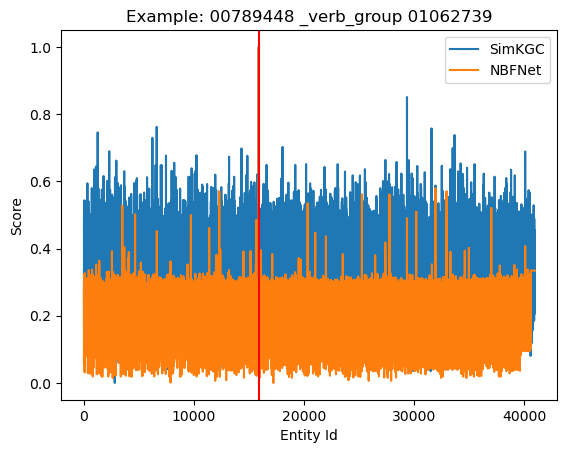
(a) Query in reachable split

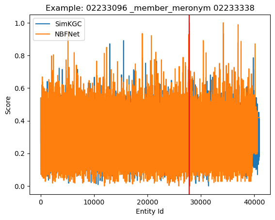
(b) Query in unreachable split

Figure 1: Score distributions of $\fol{[NBF]}$ and $\fol{[Sim]}$ for two queries in WN18RR

We notice that for the query in the reachable split, $\fol{[NBF]}$ is very confident about its top prediction. Therefore, it scores the gold answer significantly higher than the other candidates. Upon normalization, this causes the other entities to have comparatively smaller values (mostly in the range [0-0.4]), with a tighter spread. In comparison, for the query in the unreachable split, $\fol{[NBF]}$ cannot predict the gold answer confidently. This results in a much larger spread of scores across entities, with a lot of extreme values close to 1 indicating that the model is unable to conclusively determine which entity is the correct one. We choose the mean and variance as features because they will be able to distinguish between these two distributions, with their values being substantially smaller in the first case where $\fol{[NBF]}$ is confident about the predictions.

$\fol{[Sim]}$ also has these properties, albeit to a lesser degree. This is because SimKGC cannot exploit the KG structure, and therefore has to draw conclusions based on textual descriptions, which can point to several candidate answers of seemingly comparable validity. This results in the score distributions having a higher spread and a lower margin between the score of the top prediction and the other candidates. Therefore, the relative values of these mean and variance features can also inform the MLPs about the relative confidence of the models about their output, allowing them to compute ensemble weights for corresponding models as necessary.

As validation, we present the average of the mean and variance features from $\fol{[NBF]}$ over all test queries in the reachable and unreachable split for the WN18RR, FB15k-237 and CoDex-M datasets in Table 7.

Table 7: Average of$\fol{[NBF]}$ Features across Splits

Dataset	Reachable Split		Unreachable Split
	Mean	Var	Mean	Var
WN18RR	0.277	0.008	0.353	0.127
FB15k-237	0.244	0.017	0.284	0.019
CoDex-M	0.492	0.015	0.566	0.017

We find that the average of the mean and variance features is up to 21% lower (for WN18RR) on the reachable split than the unreachable split, allowing the MLPs to distinguish between the splits based on score distribution statistics alone. We also experiment with other features such as standard deviation, and mean of the top-k predictions, however we find that they do not result in substantial performance gains over the features we finally use.

Appendix D Detailed Reachability Ablation

In this section we discuss further results of the experiment done to answer Q1 in Section 5. The results presented in Table 6 are supplementary to the results presented in Table 2 where in addition to the MRR, Hits@1, Hits@10 metrics already presented in Table 2, we present results over one additional metric, MR. Additionally, we present the results on the ‘reachable’ and ‘unreachable’ split of CoDex-M, and for $\fol{[RotE]}$ and $\fol{[Comp]}$ on all datasets. We observe that $\fol{[Sim]}$ has up to 76% lower MR than $\fol{[NBF]}$ on the unreachable split while $\fol{[NBF]}$ has up to 83.3% lower MR than $\fol{[Sim]}$ on the reachable split over all the three datasets (both statistics mentioned are for WN18RR). The ensemble of $\fol{[Sim]}$+$\fol{[NBF]}$ brings the MR down further, notably obtaining a gain of 42.5% on reachable split and 66% on unreachable split over best individual models for the WN18RR dataset. We also observe that $\fol{[RotE]}$ and $\fol{[Comp]}$ show similar variation of performance across splits when compared to $\fol{[NBF]}$, performing notably better on the reachable split as compared to the unreachable split across datasets. This indicates that these KG embedding models are also dependent on KG structure and paths between the head and gold tail to some extent for performance. We investigate this in more detail in Appendix E.

Appendix E RotatE as a Structure-Based Model

We claim that despite structure not being explicitly involved in the training of $\fol{[RotE]}$, it is still capable of capturing the structure of the KG to some extent in its relation embeddings by exploiting the compositionality inherent in its scoring function. Consider an example in which $\fol{(h_{1},r_{1},h_{2})}$, $\fol{(h_{2},r_{2},h_{3})}$ and $\fol{(h_{1},r_{3},h_{3})}$ are all present in the KG. Let $\fol{T_{r}(h)}$ be the vector obtained after rotating the embedding of $\fol{h}$ by the complex rotation defined by $\fol{r}$. During training, $\fol{T_{r_{1}}(h_{1})}$ will be brought close to the embedding of $\fol{h_{2}}$ and $\fol{T_{r_{2}}(h_{2})}$ will be brought close to the embedding of $\fol{h_{3}}$. As a result, $\fol{T_{r_{2}}(T_{r_{1}}(h_{1}))}$ will be brought close to $\fol{h_{3}}$. Upon training on $\fol{(h_{1},r_{3},h_{3})}$, $\fol{T_{r_{3}}(h_{1}))}$ will also be brought close to $\fol{h_{3}}$. However, the relative positions of $\fol{h_{1}}$ and $\fol{h_{3}}$ on the complex plane already contain information about $\fol{T_{r_{2}}\circ T_{r_{1}}}$, which is used while training $\fol{T_{r_{3}}}$. As more such examples are seen over multiple epochs, $\fol{T_{r_{3}}}$ will eventually be brought closer to the composed rotation $\fol{T_{r_{2}}\circ T_{r_{1}}}$. Therefore, when query $\fol{(h,r_{3},?)}$ is seen at test time, the model will be more likely to return candidates $\fol{t}$ which are connected to $\fol{h}$ through a path in the KG involving relations $\fol{r_{1}}$ and $\fol{r_{2}}$, making it structure dependent.

Of course, this phenomenon is not limited to paths of length 2, but can encode paths of longer length as well. We also expect only the most common paths to be captured through this mechanism, since multiple such paths have to be encoded by the same relation embedding. To validate these claims, we perform an experiment where we exhaustively mine the dataset for cases where $\fol{(h_{1},r_{1},h_{2})}$ is present in the KG, alongside an entity $\fol{h_{3}}$ such that $\fol{(h_{1},r_{2},h_{3})}$ and $\fol{(h_{3},r_{3},h_{2})}$ are also present in the KG. This essentially considers all the cases where there is a path involving $\fol{r_{2}}$ and $\fol{r_{3}}$ that is closed by $\fol{r_{1}}$. We enumerate all such cases for each triple $\fol{(r_{1},r_{2},r_{3})}$ and filter out those triples that have less than 20 occurrences in the KG. For each of the remaining triples, we take a random vector and transform it according to $\fol{T_{r_{2}}\circ T_{r_{3}}}$. We then report the $\fol{r}$ such that transforming the same vector according to $\fol{T_{r}}$ moves it closest to the result obtained on transforming it according to $\fol{T_{r_{2}}\circ T_{r_{3}}}$. We expect $\fol{r}$ to be $\fol{r_{1}}$ for a majority of the triples based on our claims. We report accuracies obtained through this experiment for $\fol{[RotE]}$ on the WN18RR, FB15k-237 and CoDex-M datasets in Table 8.

Table 8: Structure Dependency of $\fol{[RotE]}$ and $\fol{[Comp]}$

Dataset	Accuracy of Closest Relation
	$\fol{[RotE]}$
WN18RR	38.1
FB15k-237	45.0
CoDex-M	68.2

We find that the accuracies are substantially better than the random baseline of $\frac{\fol{1}}{\fol{NumberofRelations}}$ for all datasets (which is 9.1% for WN18RR, 0.4% for FB15k-237 and 1.4% for CoDex-M). $\fol{[Sim]}$ is not capable of capturing this notion, since it encodes $\fol{(h,r)}$ together using BERT, not as a composition of $\fol{h}$ and $\fol{r}$ embeddings. Therefore, we find that its behavior is independent of the split in which the query under consideration is present.

Appendix F Reachability Trends of Ensemble Weights

The aim of this section is to further discuss the results of the experiment done to answer Q2 in Section 5. The results in Table 9 present the mean and standard deviation of ensemble weights $\fol{w_{2}}$ over the queries in the reachable and unreachable split for the WN18RR, CoDex-M and FB15k-237 datasets. The weight discussed in these tables is $\fol{w_{2}}$ in the ensemble defined as $\fol{w_{1}[Sim]}$ + $\fol{w_{2}[NBF]}$ (with $\fol{w_{1}}=1$) according to Section 3. We observe that across all datasets, the average weight for reachable split is higher than the weight of unreachable split (up to 17% higher for WN18RR), thus reinforcing the fact that our approach gives more weightage to $\fol{[NBF]}$ on the reachable split across datasets. The standard deviation of $\fol{w_{2}}$ is also non-trivial on all splits of all datasets, showing that our approach is capable of adjusting it as required by individual queries.

Table 9: Mean and Standard Deviation (Std Dev in Table) of Ensemble Weights for $\fol{[Sim]+[NBF]}$

Dataset	Reachable Split		Unreachable Split
	Mean	Std Dev	Mean	Std Dev
WN18RR	0.61	0.04	0.52	0.07
CoDex-M	2.03	0.24	1.91	0.38
FB15k-237	2.64	0.22	2.57	0.24

References

- Baras and Theodorakopoulos (2010) Baras S Baras and George Theodorakopoulos. 2010. Path Problems in Networks. Synthetic Lectures in Communication Networks, 3:1–77.
- Bordes et al. (2013) Antoine Bordes, Nicolas Usunier, Alberto Garcia-Duran, Jason Weston, and Oksana Yakhnenko. 2013. Translating Embeddings for Modeling Multi-relational Data. In NeurIPS. Curran Associates, Inc.
- Dettmers et al. (2018) Tim Dettmers, Pasquale Minervini, Pontus Stenetorp, and Sebastian Riedel. 2018. Convolutional 2D Knowledge Graph Embeddings. In Proceedings of the Thirty-Second AAAI Conference on Artificial Intelligence and Thirtieth Innovative Applications of Artificial Intelligence Conference and Eighth AAAI Symposium on Educational Advances in Artificial Intelligence, AAAI’18/IAAI’18/EAAI’18. AAAI Press.
- Devlin et al. (2019) Jacob Devlin, Ming-Wei Chang, Kenton Lee, and Kristina Toutanova. 2019. BERT: Pre-training of Deep Bidirectional Transformers for Language Understanding. In Proceedings of the 2019 Conference of the North American Chapter of the Association for Computational Linguistics: Human Language Technologies, Volume 1 (Long and Short Papers), pages 4171–4186, Minneapolis, Minnesota. Association for Computational Linguistics.
- Han et al. (2020) Shuguang Han, Xuanhui Wang, Michael Bendersky, and Marc Najork. 2020. Learning-to-Rank with BERT in TF-Ranking. In Arxiv.
- Mahdisoltani et al. (2015) Farzaneh Mahdisoltani, Joanna Asia Biega, and Fabian M. Suchanek. 2015. Yago3: A Knowledge Base from Multilingual Wikipedias. In Conference on Innovative Data Systems Research.
- Qu et al. (2021) Meng Qu, Junkun Chen, Louis-Pascal A. C. Xhonneux, Yoshua Bengio, and Jian Tang. 2021. RNNLogic: Learning Logic Rules for Reasoning on Knowledge Graphs. In ICLR, pages 1–21.
- Safavi and Koutra (2020) Tara Safavi and Danai Koutra. 2020. CoDEx: A Comprehensive Knowledge Graph Completion Benchmark. In Proceedings of the 2020 Conference on Empirical Methods in Natural Language Processing (EMNLP), pages 8328–8350, Online. Association for Computational Linguistics.
- Sun et al. (2019) Zhiqing Sun, Zhi-Hong Deng, Jian-Yun Nie, and Jian Tang. 2019. RotatE: Knowledge Graph Embedding by Relational Rotation in Complex Space. In ICLR.
- Toutanova and Chen (2015) Kristina Toutanova and Danqi Chen. 2015. Observed versus Latent Features for Knowledge Base and Text Inference. In Proceedings of the 3rd Workshop on Continuous Vector Space Models and their Compositionality, pages 57–66, Beijing, China. Association for Computational Linguistics.
- Trouillon et al. (2016) Théo Trouillon, Johannes Welbl, Sebastian Riedel, Éric Gaussier, and Guillaume Bouchard. 2016. Complex Embeddings for Simple Link Prediction. In ICML, page 2071–2080. JMLR.org.
- Wang et al. (2022) Liang Wang, Wei Zhao, Zhuoyu Wei, and Jingming Liu. 2022. SimKGC: Simple Contrastive Knowledge Graph Completion with Pre-trained Language Models. In Proceedings of the 60th Annual Meeting of the Association for Computational Linguistics (Volume 1: Long Papers), pages 4281–4294, Dublin, Ireland. Association for Computational Linguistics.
- Yao et al. (2019) Liang Yao, Chengsheng Mao, and Yuan Luo. 2019. KG-BERT: BERT for Knowledge Graph Completion. In AAAI Conference on Artificial Intelligence.
- Zhang et al. (2020) Zhao Zhang, Fuzhen Zhuang, Hengshu Zhu, Zhi-Ping Shi, Hui Xiong, and Qing He. 2020. Relational Graph Neural Network with Hierarchical Attention for Knowledge Graph Completion. In The Thirty-Fourth AAAI Conference on Artificial Intelligence, pages 9612–9619. AAAI Press.
- Zhu et al. (2021) Zhaocheng Zhu, Zuobai Zhang, Louis-Pascal Xhonneux, and Jian Tang. 2021. Neural Bellman-Ford Networks: A General Graph Neural Network Framework for Link Prediction. In Advances in Neural Information Processing Systems.