Beyond Traditional Beamforming: Singular Vector Projection Techniques for MU-MIMO Interference Management

Abstract

This paper introduces low-complexity beamforming algorithms for multi-user multiple-input multiple-output (MU-MIMO) systems to minimize inter-user interference and enhance spectral efficiency (SE). A Singular-Vector Beamspace Search (SVBS) algorithm is initially presented, wherein all the singular vectors are assessed to determine the most effective beamforming scheme. We then establish a mathematical proof demonstrating that the total inter-user interference of a MU-MIMO beamforming system can be efficiently calculated from the mutual projections of orthonormal singular vectors. Capitalizing on this, we present an Interference-optimized Singular Vector Beamforming (IOSVB) algorithm for optimal singular vector selection. For further reducing the computational burden, we propose a Dimensionality-reduced IOSVB (DR-IOSVB) algorithm by integrating the principal component analysis (PCA). The numerical results demonstrate the superiority of the SVBS algorithm over the existing algorithms, with the IOSVB offering near-identical SE and the DR-IOSVB balancing the performance and computational efficiency. This work establishes a new benchmark for high-performance and low-complexity beamforming in MU-MIMO wireless communication systems.

I Introduction

The surge in demand for robust wireless communication has highlighted massive multiple-input multiple-output (MIMO) as a vital technology [1]. Utilizing a multitude of antennas at the base station (BS), it promises heightened performance in wireless systems [2]. This technology, introduced in 2010 by Marzetta [3], boasts capabilities such as high spectral efficiency (SE) and reduced interference, finding its application extensively in 5G systems.

Multi-user MIMO (MU-MIMO) emerged to meet higher data rates and network capacity demands [4]. Yet, inter-user interference remains an impediment to reaping MU-MIMO’s full benefits [5]. Various researchers have sought efficient beamforming algorithms to manage this interference in MU-MIMO systems [6]. However, many algorithms exhibit high computational complexity, making real-time implementation in vast systems challenging.

A plethora of studies have examined beamforming for MU-MIMO. These encompass low-complexity precoding, joint spatial division, multiplexing strategies, and unique codebook designs, among others. Specific notable contributions include coordinated beamforming [7], hybrid precoding schemes [8], spatial division-multiplexing [9], linear precoding under feedback constraints [10] and dynamic user clustering strategy [11]. A hybrid beamforming based on compress sensing on feedback channel state information (CSI) is proposed by Jing et al. [12], where the digital beamformer is optimized using the Zero Forcing (ZF) algorithm and the analog beamformer is optimized using the Conjugate Transpose algorithm. Ahmed et al. in [13] also proposed a hybrid beamforming based on the QR decomposition method. Garcia et al. in [14] propose a DFT-based, fully-connected analog beamforming network in which the digital precoder is optimized using the ZF algorithm. Nguyen et al. [15] proposed an OMP-based algorithm that transmits array response vectors under the assumption of perfect Angle of Departure (AoD) knowledge, and the sum-MSE algorithm is used to find the digital beamformer. Also, in [16], the authors proposed a new beamforming technique based on Manifold optimization and ZF algorithm, in which they attempted to reduce the optimization time compared to the existing algorithms with a minimal loss in SE.

Several other works such as Eigen beamforming [17], Linear Precoding [18], Subspace construction algorithm [19], and Phased ZF [20] were able to achieve high SE whilst also adopting a single antenna per user in their system models, in contrast to our configuration where we assume multiple antennae per user. Also, other algorithms such as Higher-order SVD [21], continuous aperture phased-MIMO [22], and subarray wise iterative algorithm [8], ZF beamforming algorithm based on Monte-Carlo simulation [23] and basis pursuit based solutions [24, 25, 26] perform well in term of SE. However, these algorithms are based on the single-user MIMO system model and cannot be employed in multi-user MIMO scenarios.

In [27], the authors proposed a new hybrid precoding implementation for millimeter wave (mmWave) systems, utilizing a small number of fixed phase shifters (FPS) with quantized phases. This cost-effective approach significantly reduces hardware complexity while maintaining high SE. In [15], the authors studied hybrid precoding for multiuser mmWave systems and developed a new hybrid minimum mean-squared error (MMSE) precoder. The proposed precoder, obtained through an orthogonal matching pursuit-based algorithm, demonstrated significant performance advantages over known designs in various system settings. In [28], the authors proposed effective alternating minimization (AltMin) algorithms for hybrid precoding in mmWave MIMO systems, focusing on fully-connected and partially-connected structures. The proposed AltMin algorithms demonstrated significant performance gains over the existing hybrid precoding algorithms and provided valuable design insights.

Existing beamforming algorithms for multi-user massive MIMO systems often rely on numerical iteration-based complex computations, which hinder real-time resource allocation and generate substantial computational overhead, increasing both latency and costs [29, 30, 31, 32]. Moreover, these algorithms are often valid only for specific network configurations, and their computational costs escalate as the number of antennas in massive MIMO systems increases. Traditional maximum ratio (MR) and MMSE algorithms utilized in MIMO receivers do not prioritize reducing computational complexity and communication latency. In addition, the Codebook searching method, widely used in hybrid beamforming [33, 34], has a high computational complexity despite providing high SE. As a result, there is a critical need for low-complexity algorithms that effectively minimize inter-user interference, improve signal-to-interference plus noise ratio (SINR), and provide high SE.

This paper considers a downlink MU-MIMO beamforming system with one BS and multiple users. We propose low-complexity beamforming algorithms that address the challenges associated with inter-user interference management for providing high SE. The proposed approach builds upon recent advancements in the field and incorporates dimensionality-reduced and projection-based techniques for efficient interference measurement. The major contributions in this paper are as follows:

• We introduce an exhaustive search algorithm, the Singular-Vector Beamspace Search (SVBS). Our results demonstrate its superiority over conventional MMSE and ZF-based methods in multi-user contexts, providing a solid baseline for comparing the SE of lower-complexity algorithms.

• We establish the equivalence of inter-user interference to mutual projections between singular vectors. Leveraging this, we present a low-complexity Interference Optimized Singular Vector Beamforming (IOSVB) algorithm which significantly reduces computational demands while preserving SE.

• A dimensionality-reduced IOSVB (DR-IOSVB) algorithm, inspired by PCA, is proposed to curtail the complexity of interference measurements further, making it more adaptable for real-time, large-scale implementations.

• We offer solutions for hybrid beamforming parameters using the IOSVB algorithm.

The rest of the paper is organized as follows. MU-MIMO system, including channel modeling, is described, and the problem is formulated in Section II. The proposed beamforming algorithms are presented in Section III. We present and analyze the numerical results in Section IV. Section V concludes the paper.

Notation: Scalars, matrices, and vectors are represented in lower case, bold upper, and bold lower cases, respectively. Scalar norms, vector $L_{2}$ norms, and Frobenius norms are denoted by $|.|$, $||.||$, and $||.||_{F}$, respectively. For any general matrix or vector operator x, x^T and x^* represent the transpose and conjugate transpose matrices, respectively. E[.], $\mathbb{C}$ and $\mathbb{N}$ denote the expected value, the set of the complex and natural numbers, respectively.

TABLE I: Summary of Important Notations

Notation	Definition
Hk	Channel matrix for $k$-th user
$N_{t}$ , $N_{r}$	Number of transmit and receive antennas
U	Number of users
$N_{s}$	Number of data streams transmitted
	to each users
$N^{t}_{RF}$	Number of RF chains at transmitter
$N^{r}_{RF}$	Number of RF chains at receiver
$\textbf{s}_{k}$	Symbol vector of $k$-th user
$\mathbf{\Delta}_{k}$	Interference of the $k$-th user for a
	hybrid system
$\mathbf{\Delta}^{D}_{k}$	Interference of the $k$-th user for a fully
	digital system
FA, FkD	Analog and digital beamforming matrices
	at transmit end
WkA, WkD	Analog and digital beamforming matrices at
	receiver end
Uk, Vk	Two orthonormal matrices found by
	SVD of Hk
$\bm{\Sigma_{k}}$	The diagonal matrix found by
	SVD of $\bm{H_{k}}$
$R_{sel}$	Number of selected columns taken
	from $\textbf{U}_{k}$ and $\textbf{V}_{k}$
$\mathbf{ind}^{i}$	Array index for $i$-th iteration
$\textbf{F}^{k}_{sel}$, $\textbf{W}^{k}_{sel}$	Transmit and receive beamforming
	candidate matrices
$\textbf{F}^{sel}$, $\textbf{W}^{sel}$	Combined transmit and receive beamforming
	candidate matrices
$\textbf{F}^{o}_{k}$, $\textbf{W}^{o}_{k}$	Optimal fully digital precoding and
	combining matrices for $k$-th user
$\textbf{F}^{o}$, $\textbf{W}^{o}$	Combined optimal fully digital precoding
	and combining matrices
$\textbf{C}^{sel}$	Combined correlation matrix
$\sigma_{sel}$	Selected minimum channel gain threshold
$\mathbf{C}_{corr}^{i}$	Correlation matrix for i-th combination
$\mathbf{F}^{io}$, $\mathbf{W}^{io}$	Optimized fully digital beamforming matrices
$I_{t}$	Total interference of the system
$\gamma$	Channel gain threshold

II System Model and Problem Formulation

In this section, we describe the MU-MIMO beamforming system and channel model. We then formulate the basic multi-user beamforming problem.

II-A System Model

We consider a downlink MU-MIMO system consisting of $U$ number of users, each employed with $N_{r}$ number of receiving antennas. A BS with $N_{t}$ transmit antennas is used to serve $N_{s}$ data streams to each user. The number of RF chains at the BS is denoted as $N_{RF}^{t}$, where $N_{RF}^{t}\geq UN_{s}$, and the number of RF chains at the user equipment (UE) is denoted as $N_{RF}^{r}$, where $N_{RF}^{r}\geq N_{s}$. We assume a fully connected hybrid architecture as shown in Fig. 1.

The transmitted signal at the BS can be written as $\textbf{x}=\textbf{F}^{A}\textbf{F}^{D}\textbf{s}$, where s is a vector of data symbol of length $UN_{s}$, $\textbf{F}^{A}$ is the analog beamforming matrix at the BS, and $\textbf{F}^{D}$is the digital beamforming matrix at the BS. Note that $\textbf{F}^{A}$ is a $N_{t}\times N_{RF}^{t}$ matrix and $\textbf{F}^{D}$ is a $N_{RF}^{t}\times UN_{s}$ matrix. Further, the digital beamforming matrix for the k-th user is symbolized as $\textbf{F}_{k}^{D}$, which is a $N_{RF}^{t}\times N_{s}$ matrix. Let $\textbf{H}_{k}$ be channel matrix for $k^{th}$ user with dimension $N_{r}\times N_{t}$. Further, let $\textbf{W}_{k}^{A}$ be the $N_{r}\times N_{RF}^{r}$ analog beamforming matrix and $\textbf{W}_{k}^{D}$ be the $N_{RF}^{r}\times N_{s}$ digital beamforming matrix for $k^{th}$ user at the UE. The non-zero elements of analog beamforming matrices $\textbf{F}^{A}$ and $\textbf{W}_{k}^{A}$ have unit modulus constraints because analog pre-coders are implemented using phase shifters which change the phases without contributing to the magnitude. A summary of the important notations is provided in Table I.

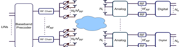
Figure 1: Block diagram of transmitter and receiver for the system.

II-B Channel Model

We consider the Saleh-Valenzuela model for channel design, which is a statistical, cluster-based channel model [35, 36] extensively employed in mmWave applications. It connects the clustering phenomena with the stochastic angles of departure/arrival for each beam [37]. The channel vector for $k^{th}$ user can be written as

$$\textbf{H}_{k}=\sqrt{\frac{N_{t}N_{r}}{L_{k}}}\;\;\sum_{i=1}^{L_{k}}\alpha_{k,i}\;\textbf{a}_{r}(\phi_{k,i}^{r},\theta_{k,i}^{r})\;\textbf{a}_{t}^{H}(\phi_{k,i}^{t},\theta_{k,i}^{t}),$$ (1)

where, $L_{k}$ is the number of propagation paths for the $k$-th user, $\alpha_{k,i}$ $\in$ $\mathbb{C}$ is the channel gain of $k$-th user of the $i$-th path that follows complex Gaussian distribution and $\textbf{a}_{r}(\phi_{k,i}^{r},\theta_{k,i}^{r})$ and $\textbf{a}_{t}(\phi_{k,i}^{t},\theta_{k,i}^{t})$ are the normalized receive and transmit array response vectors, respectively. Moreover, $\phi_{k,i}^{t}$ and $\theta_{k,i}^{t}$ are the azimuth and elevation angles of the angle of departure (AOD), and $\phi_{k,i}^{r}$ and $\theta_{k,i}^{r}$ are the azimuth and elevation angles of the angle of arrival (AOA). Here, the matrices $\Phi_{k,i}^{t}$ and $\Theta_{k,i}^{t}$ follow Zero-Mean Second Order Gaussian Mixture Model [38]. A normalization factor $N_{t}N_{r}$ is added to (1) for satisfying $\operatorname{\mathbb{E}}{\{{||\textbf{H}_{k}||}_{F}^{2}\}}=N_{t}N_{r}$.

II-C Problem Formulation

II-C1 SINR and Data Rate Modelling

The transmitted signal for the $k$-th user at the BS can be expressed as

$$\textbf{x}_{k}=\textbf{F}^{A}\textbf{F}_{k}^{D}\textbf{s}_{k},$$ (2)

where, $\textbf{s}_{k}$ is the vector containing $N_{s}$ symbols. The received signal at the $k$-th receiver can be writtem as

$$\textbf{r}_{k}=\textbf{H}_{k}\textbf{F}^{A}\textbf{F}_{k}^{D}\textbf{s}_{k}+\sum_{i=1,i\neq k}^{U}\textbf{H}_{k}\textbf{F}^{A}\textbf{F}_{i}^{D}\textbf{s}_{i}+\textbf{n}_{k},$$ (3)

where, $\textbf{n}_{k}$ is the AWGN noise vector of size $N_{r}\times 1$ for the $k$-th user. After combining at the receiver end, i.e., by multiplying the beamforming matrices, the received signal for $k$-th user can be obtained as

$$\textbf{y}_{k} ={(\textbf{W}_{k}^{D})}^{H}{(\textbf{W}_{k}^{A})}^{H}\textbf{H}_{k}\textbf{F}^{A}\textbf{F}_{k}^{D}\textbf{s}_{k}$$

$$+\sum_{i=1,i\neq k}^{U}{(\textbf{W}_{k}^{D})}^{H}{(\textbf{W}_{k}^{A})}^{H}\textbf{H}_{k}\textbf{F}^{A}\textbf{F}_{i}^{D}\textbf{s}_{i}$$

$$+{(\textbf{W}_{k}^{D})}^{H}{(\textbf{W}_{k}^{A})}^{H}\textbf{n}_{k},$$ (4)

where, the first term on the right-hand side is the desired signal, the second term is the interference, and the third term is the noise. In this case, the interference between two data streams of the same user is not considered as the BS transmits the data streams of the $k$-th user in such a way that they are orthonormal to one another and thus nulling out the interference between the $k$-th user’s adjacent data streams. Let the total interference caused by the other users to the user $k$ be ${\Delta}_{k}$. Thus,

$${\Delta}_{k}=\sum_{i=1,i\neq k}^{U}|{(\textbf{W}_{k}^{D})}^{H}{(\textbf{W}_{k}^{A})}^{H}\textbf{H}_{k}\textbf{F}^{A}\textbf{F}_{i}^{D}|^{2}.$$ (5)

Now, the SINR for the $k$-th user can be written as

$$SINR_{k}=\frac{|{(\mathbf{W}_{k}^{D})}^{H}{(\textbf{W}_{k}^{A})}^{H}\textbf{H}_{k}\textbf{F}^{A}\textbf{F}_{k}^{D}|^{2}}{{\Delta}_{k}+|{(\textbf{W}_{k}^{D})}^{H}{(\textbf{W}_{k}^{A})}^{H}\textbf{n}_{k}|^{2}}.$$ (6)

The data rate per Hertz for the $k$-th user can be written as

$$R_{k}=\log_{2}(1+SINR_{k}),$$ (7)

and the sum-rate of the system per Hertz can be found as

$$R=\sum_{k=1}^{U}R_{k},$$ (8)

which is also called the SE.

II-C2 Beamforming Solution for SU-MIMO

Assume that the $k$-th user is the only one that exists in the system. The channel matrix of $k$-th user can be decomposed using Singular Value Decomposition (SVD) as follows

$$\textbf{H}_{k}=\textbf{U}_{k}\mathbf{\Sigma}_{k}\textbf{V}_{k}^{H},$$ (9)

where, $\textbf{U}_{k}$ and $\textbf{V}_{k}$ are both orthonormal matrices and the diagonal matrix $\mathbf{\Sigma}_{k}$ can be written as, $diag(\sigma_{k}^{1},\sigma_{k}^{2},\sigma_{k}^{3},\ldots,\sigma_{k}^{N_{t}})$, where, $\sigma_{k}^{1}>\sigma_{k}^{2}>\sigma_{k}^{3}>\ldots>\sigma_{k}^{N_{t}}$. In the scenario of a single-user system, the optimal digital precoding matrix at the BS of the $k$-th user $\textbf{F}^{opt}_{k}$ is calculated as $\textbf{F}^{opt}_{k}=\textbf{V}_{k{[1:N_{s}]}}^{H}$, where first $N_{s}$ number of columns are taken from $\textbf{V}_{k}^{H}$ matrix to transmit $N_{s}$ data streams for a user. Also, the optimal combining matrix for the $k$-th user can be written as $\textbf{W}^{opt}_{k}$, which is calculated as $\textbf{W}^{opt}_{k}=\textbf{U}_{k[1:N_{s}]}$. Note that in a single-user scenario, where there is no multi-user interference in the system, $\textbf{F}^{opt}_{k}$ and $\textbf{W}^{opt}_{k}$ provide the optimal sum rate[27]. As for hybrid beamforming design, one needs to find out the analog and digital beamforming matrices for both the precoder and combiner. For finding the hybrid beamforming matrices, traditional beamforming algorithms [27, 39, 28] and deep-learning-based ones [40] minimize the difference of the product of hybrid beamforming matrices with optimal beamforming matrix so that the hybrid beamforming matrices are close to the optimal beamforming matrics, and thus maximizing the sum-rate of the system. Therefore, for the transmit end, the goal is minimizing the value of $||\textbf{F}^{opt}_{k}-\textbf{F}^{A}\textbf{F}^{D}_{k}||$. Now for the receiver end of the $k$-th user, the objective is to minimize the value of $||\textbf{W}^{opt}_{k}-\textbf{W}^{A}_{k}\textbf{W}^{D}_{k}||$.

Traditional methods often select the first $N_{s}$ columns from $\textbf{V}_{k}^{H}$ demonstrating the highest channel gain. While effective in single-user settings, this might not be optimal in multi-user scenarios. In multi-user environments, maximizing channel gain might also result in high interference with other users’ beams, thus decreasing the overall sum rate. Hence, it’s essential not just to focus on maximizing the channel gain but also to consider potential interference in beam selection for optimizing the sum rate in multi-user systems.

II-C3 Problem Definition for MU-MIMO System

There are some iteration based algorithms which consider interference [41, 42] as they optimize the sum-rate or SE. However, the computational efficiencies of those algorithms are very poor. Therefore, the maximization of SE while taking interference into account in a time-efficient manner is a critical problem.

Let the optimum selection matrices be $\textbf{F}^{io}$ and $\textbf{W}^{io}$ that contain the beam directions, which minimize the interference between the adjacent beams of the other users. Note that both $\textbf{F}^{io}$ and $\textbf{W}^{io}$ are the combinations of analog and digital beamforming, i.e., $\textbf{F}^{io}$ represents the optimal beam direction for $\textbf{F}^{\mathrm{A}}\textbf{F}^{\mathrm{D}}$ and $\textbf{W}^{io}$ represents the optimal beam direction for $\textbf{W}^{\mathrm{A}}\textbf{W}^{\mathrm{D}}$. Here, $\textbf{F}^{io}$ is a $N_{t}\times UN_{s}$ matrix that consists of $UN_{s}$ columns, each indicating one specific direction for transmitting the beams. Also, $\textbf{W}^{io}$ is a $N_{r}\times UN_{s}$ matrix, the combiner matrix for $UN_{s}$ data streams. Note that, $\textbf{F}^{io}_{k}$ is a $N_{t}\times N_{s}$ matrix for the $k$-th user, that can be found as, $\textbf{F}^{io}=\{\textbf{F}_{1}^{io},\textbf{F}_{2}^{io},\cdots,\textbf{F}_{k}^{io},\cdots,\textbf{F}_{U}^{io}\}$. Similarly, $\textbf{W}_{k}^{io}$ is a $N_{r}\times N_{s}$ matrix for the $k$-th that can be calculated as, $\textbf{W}^{io}=\{\textbf{W}_{1}^{io},\textbf{W}_{2}^{io},\cdots,\textbf{W}_{k}^{io},\cdots,\textbf{W}_{U}^{io}\}$. With $\textbf{F}^{io}$ and $\textbf{W}^{io}$, the data rate can be obtained as

$$R_{D}=\sum_{k=1}^{U}\log_{2}(1+\frac{|{(\textbf{W}_{k}^{io})}^{H}\textbf{H}_{k}\textbf{F}_{k}^{io}|^{2}}{\Delta^{D}_{k}+|{(\textbf{W}_{k}^{io})}^{H}\textbf{n}_{k}|^{2}}),$$ (10)

where, $\Delta^{D}_{k}=\sum_{i=1,i\neq k}^{U}|{(\textbf{W}_{k}^{io})}^{H}\textbf{H}_{k}\textbf{F}_{k}^{io}|^{2}$ is the interference for the $k$-th user.

We divide the sum-rate maximization problem into two sub-problems. The first sub-problem is to find the matrices $\textbf{F}_{k}^{io}$ and $\textbf{W}_{k}^{io}$ to minimize the interference and maximize the sum rate. Thus, the sub-problem is to find $\textbf{F}^{io}$ from all the combinations in ${\{\textbf{V}_{k}^{H}\}}_{k=1}^{U}$ and $\textbf{W}^{io}$ from all the combinations in ${\{\textbf{U}_{k}^{H}\}}_{k=1}^{U}$ so that $R_{D}$ is maximized. After solving both the transmit and receiver end beamforming matrices $\textbf{F}^{io}$ and $\textbf{W}^{io}$, the second sub-problem is to find the hybrid precoding and combining matrices for the BS and the UEs. Thus, the sub-problem is to find out the analog precoding matrix $\textbf{F}_{A}$ and digital precoding matrix $\textbf{F}^{D}$ in the BS, along with the beamforming matrices $\textbf{W}_{A}$ and $\textbf{W}^{D}$ at the UE. So, there are two optimization problems for the second sub-problem. The first optimization problem can be written as

$$\underset{\mathbf{F}^{\mathrm{A}},\mathbf{F}^{\mathrm{D}}}{\operatorname{min}}\;\;{\|\mathbf{F}^{\mathrm{io}}-\mathbf{F}^{\mathrm{A}}\mathbf{F}^{\mathrm{D}}\|}_{F}^{2}$$ (11)

$$\text{Subject to}\begin{cases}|{(\mathbf{F}^{\mathrm{A}})}_{i,j}|=1\\ {\|\mathbf{F}^{\mathrm{A}}\mathbf{F}^{\mathrm{D}}\|}_{F}^{2}=UN_{s}.\end{cases}$$

Similarly, the second optimization problem can be written as

$$\underset{\mathbf{W}^{\mathrm{A}},\mathbf{W}^{\mathrm{D}}}{\operatorname{min}}\;\;{\|\mathbf{W}^{\mathrm{io}}_{\mathrm{k}}-\mathbf{W}^{\mathrm{A}}_{\mathrm{k}}\mathbf{W}^{\mathrm{D}}_{\mathrm{k}}\|}_{F}^{2}$$ (12)

$$\text{Subject to}\begin{cases}|{(\mathbf{W}^{\mathrm{A}}_{\mathrm{k}})}_{i,j}|=1\\ {\|\mathbf{W}^{\mathrm{A}}_{\mathrm{k}}\mathbf{W}^{\mathrm{D}}_{\mathrm{k}}\|}_{F}^{2}=N_{s}.\end{cases}$$

III Proposed Beamforming Algorithms

In this section, we introduce four algorithms to maximize sum-rate or SE. Firstly, the SVBS algorithm performs an exhaustive search of optimal beamforming vectors by evaluating all singular vectors. Secondly, the IOSVB algorithm, a low-complexity solution, estimates inter-user interference through channel singular vector correlation, aiming to minimize interference and boost data rate and SE. Thirdly, we adapt existing methods to compute hybrid beamforming parameters from the full digital matrices derived from IOSVB. Lastly, the DR-IOSVB algorithm utilizes PCA to streamline the channel singular vector dimensions, simplifying interference measurement.

III-A Singular-Vector Beamspace Search (SVBS) Algorithm

It is an exhaustive search algorithm designed to compute the fully digital beamforming matrices for multi-user scenarios which may be used to determine the upper bound of SE in the case of the MU-MIMO system. In cases where a BS has $N_{t}$ transmit antennas, there are $\binom{N_{t}}{Ns}$ potential ways of transmission to serve a user with $N_{s}$ data streams. From (9), it is evident that the channel matrix of the $k$-th user can be decomposed as $\textbf{U}_{k}\mathbf{\Sigma}_{k}\textbf{V}_{k}^{H}$. Each row of $\textbf{U}_{k}$ and each column of $\textbf{V}_{k}$ represent the channel between the corresponding transmit and receive antennas, and the associated diagonal value of $\bm{\Sigma}_{k}$ indicating the channel gain of transmission. In a scenario where a BS serves $U$ users each with $N_{s}$ data streams, the search space encompasses ${\binom{N_{t}}{Ns}}^{U}$ unique combinations. For MIMO or Massive-MIMO system models featuring large antenna arrays at the BSs and a moderate number of users, searching the entire space becomes infeasible.

To address this issue, we aim to reduce the search space by eliminating the channels with negligible channel gain, as they are unlikely to enhance the data rate when utilized. Consequently, we select the first $R_{sel}$ columns instead of the entire $N_{t}$ columns from the $\textbf{V}_{k}^{H}$ matrix, where $R_{sel}\geq N_{s}$. By opting for $R_{sel}$ rather than $N_{t}$ columns, the search space is reduced to ${\binom{R_{sel}}{N_{s}}}^{U}$ combinations, making the problem more tractable. For each user, $\textbf{F}^{k}_{sel}\in C^{N_{t}\times R_{sel}}$ is selected from $\textbf{V}_{k}^{H}$ by selecting the first $R_{sel}$ columns. Similarly, $\textbf{W}^{k}_{sel}\in C^{N_{r}\times R_{sel}}$ is also selected from $\textbf{U}_{k}$ by choosing the first $R_{sel}$ columns, that can also be written as follows,

$$\textbf{F}^{sel}_{k}=\textbf{V}_{k[1:R_{sel}]}^{H},$$ (13)

$$\textbf{W}^{sel}_{k}=\textbf{U}_{k[1:R_{sel}]}.$$ (14)

Here, $R_{sel}$ is the number of potential candidate columns or beam directions for each user. Also note that the $R_{sel}$ is dependent on channel gain, which will be discussed further in later sections, and the subscript $[1:n]$ indicates the first $n$ columns of a matrix. Note that $\textbf{V}_{k}^{H}$ and $\textbf{U}_{k}$ are both ortho-normal.
Let the optimal fully digital precoding and combining matrices for the multi-user scenarios are $\textbf{F}_{k}^{o}$ and $\textbf{W}_{k}^{o}$, respectively. The optimal sum-rate of a system is provided by the matrices $\textbf{F}_{k}^{o}$ and $\textbf{W}_{k}^{o}$, which have dimensions of $N_{t}\times N_{s}$ and $N_{r}\times N_{s}$, respectively.

For the user $k$, the received signal after processing can be obtained as

$${\textbf{y}_{k}}={(\mathbf{W}_{k}^{o})}^{H}\mathbf{H}_{k}\mathbf{F}_{k}^{o}{\mathbf{s}_{k}}+{\sum_{i=1,i\neq k}^{U}{(\mathbf{W}_{k}^{o})}^{H}\mathbf{H}_{k}\mathbf{F}_{i}^{o}\mathbf{s_{k}}+{(\mathbf{W}_{k}^{o})}^{H}\mathbf{n}_{k}}.$$ (15)

Thus, the sum-rate or SE for the selected beamforming matrices is given by

$$R_{o}=\sum_{k=1}^{U}\log_{2}(1+\frac{|{(\textbf{W}_{k}^{o})}^{H}\textbf{H}_{k}\textbf{F}_{k}^{o}|^{2}}{\sum_{i=1,i\neq k}^{U}|{(\textbf{W}_{k}^{o})}^{H}\textbf{H}_{k}\textbf{F}_{i}^{o}|^{2}+|{(\textbf{W}_{k}^{o})}^{H}\textbf{n}_{k}|^{2}}).$$ (16)

We conduct an exhaustive search over the entire reduced search space to find out the precoding matrix $\textbf{F}^{o}_{k}$ and the corresponding combining matrix $\textbf{W}^{o}_{k}$ so that optimal rate $R_{o}$ can be obtained.
It is important to note that for each possible precoding matrix $\textbf{F}^{o}_{k}$ formed by taking a certain combination of singular vectors from $\textbf{V}_{k[1:R_{sel}]}$, there is one and only one corresponding combining matrix $\textbf{W}^{o}_{k}$, which is formed by taking the exact same combination of singular vectors from $\textbf{U}_{k[1:R_{sel}]}$. For example, if $\textbf{F}^{o}_{k}$ is formed by taking the first and third singular vectors from $\textbf{V}_{k[1:R_{sel}]}$ for $N_{s}=2$, then $\textbf{W}^{o}_{k}$ must also be formed by taking the first and third singular vectors from $\textbf{U}_{k[1:R_{sel}]}$. Moreover, combined optimal filly digital precoding and combining matrices $\textbf{F}^{o}$ and $\textbf{W}^{o}$ can be found as follows,

$$\textbf{F}^{o}={[\textbf{F}_{1}^{o},\textbf{F}_{2}^{o},\cdots,\textbf{F}_{k}^{o},\cdots,\textbf{F}_{U}^{o}]},$$ (17)

$$\textbf{W}^{o}={[\textbf{W}_{1}^{o},\textbf{W}_{2}^{o},\cdots,\textbf{W}_{k}^{o},\cdots,\textbf{W}_{U}^{o}]}.$$ (18)

Let us define ‘$\textbf{ind}_{k}$’ as an array of the index for $k$-th user, where each entry corresponds to the index of the selected singular vectors from $\textbf{F}^{sel}_{k}$ to construct $\textbf{F}^{o}_{k}$. Formally, this is denoted as $\textbf{F}^{sel}_{k}[\textbf{ind}_{k}]=\textbf{F}^{o}_{k}$, which implies $\textbf{F}^{o}_{k}\subseteq\textbf{F}^{sel}_{k}$. Furthermore, let $\textbf{ind}_{1}$, $\textbf{ind}_{2}$, $\textbf{ind}_{3}$ and so on represent the individual arrays of selected indices of singular vectors for each user $k\in\{1:U\}$. Consequently, the comprehensive selection index array ‘ind’ can be expressed as $\textbf{ind}=\{\textbf{ind}_{1},\textbf{ind}_{2},....,\textbf{ind}_{U}\}$. Now the combined optimal fully digital beamforming matrices $\textbf{F}^{o}$ and $\textbf{W}^{o}$ can be calculated as,

$$\textbf{F}^{sel}[\textbf{ind}]=\textbf{F}^{o};\;\;\textbf{W}^{sel}[\textbf{ind}]=\textbf{W}^{o}.$$ (19)

Here, $\textbf{F}^{sel}$ and $\textbf{W}^{sel}$ are the combined candidate matrices that are found by concatenating corresponding precoding and combining matrices for all users. That is alternatively be expressed as $\textbf{F}^{sel}=[\textbf{F}^{sel}_{1},\textbf{F}^{sel}_{2},\cdots,\textbf{F}^{sel}_{k},\cdots,F^{sel}_{U}]$ and $\textbf{W}^{sel}=[\textbf{W}^{sel}_{1},\textbf{W}^{sel}_{2},\cdots,\textbf{W}^{sel}_{k},\cdots,\textbf{W}^{sel}_{U}]$.

We present the SVBS algorithm in Algorithm 1, where $\textbf{H}_{k}$ is taken as the input and after checking ${\binom{R_{sel}}{N_{s}}}^{U}$ number of different combinations in a brute force approach, $\textbf{F}_{o}$ and $\textbf{W}_{o}$ are selected as output. Those combined optimal fully digital beamforming matrices $\textbf{F}^{o}$ and $\textbf{W}^{o}$ are used to generate optimal fully digital beamforming matrices $\textbf{F}^{o}_{k}$ and $\textbf{W}^{o}_{k}$. In algorithm 1, we form ${(\binom{R_{sel}}{N_{s}})}^{U}$ number of index arrays ind that needs to be checked by iteration. Here, $\textbf{ind}^{t}$ represents the index array of the $t$-th iteration.

Algorithm 1 Singular-Vector Beamspace Search (SVBS) Algorithm

1:Input: $\{\textbf{H}_{k}\}_{k=1}^{U}$, $N_{s}$, $R_{sel}$;

2:Find, $[\textbf{U}_{k},\mathbf{\Sigma}_{k},\textbf{V}_{k}^{H}]=SVD(\textbf{H}_{k})$ $\forall k\in\{1,2,...,U\}$;

3:Find $\textbf{F}^{sel}_{k}$ and $\textbf{W}^{sel}_{k}$ using equation 13, for user k=1:U;

4:Calculate $\textbf{F}^{sel}$ and $\textbf{W}^{sel}$ using the $\textbf{F}^{sel}_{k}$ and $\textbf{W}^{sel}_{k}$ matrices of previous step;

5:Set $R_{max}=0$;

6:Set t=0;

7:Form $\textbf{ind}^{t}$ dissimilar arrays;

8:repeat

9:     Calculate $\textbf{F}^{o}=\textbf{F}^{sel}[\textbf{ind}^{t}]$ and $\textbf{W}^{o}=\textbf{W}^{sel}[\textbf{ind}^{t}]$;

10:     Find optimal fully digital matrices ${\{\textbf{F}^{o}_{k}\}}_{k=1}^{U}$ and ${\{\textbf{W}^{o}_{k}\}}_{k=1}^{U}$ using (17) and (18);

11:     Calculate $R^{t}$ using an unique set of $\textbf{F}^{o}_{k}$ and $\textbf{W}^{o}_{k}$ matrices formed using (16);

12:     If $R^{t}>R_{max}$, set $R_{max}=R^{t}$ and $\textbf{ind}=\textbf{ind}^{t}$;

13:     $t\leftarrow t+1$;

14:until $t>\binom{R_{sel}}{N_{s}}^{U}$

15:Set $\textbf{F}^{o}=\textbf{F}^{sel}[\textbf{ind}]$ and $\textbf{W}^{o}=\textbf{W}^{sel}[\textbf{ind}]$ respectively, which corresponds to $R_{max}$.

III-B Interference Optimized Singular Vector Beamforming (IOSVB) Algorithm

This subsection describes the singular vector projections method for determining the fully digital precoder. We also provide an algorithm for determining the hybrid beamforming matrices consisting of analog and digital components.

In section III-A, we presented a strategy to derive the optimal fully digital beamforming matrices $\textbf{F}_{k}^{o}$ and $\textbf{W}_{k}^{o}$, which necessitates an exhaustive search of the entire space. Although comprehensive, this approach is time-consuming and introduces high computational complexity to the system. Therefore, in this subsection, we introduce an alternative algorithm that identifies the near-optimal fully digital beamforming matrices, $\textbf{F}^{io}$ and $\textbf{W}^{io}$, from the candidate matrices $\textbf{F}^{sel}$ and $\textbf{W}^{sel}$, respectively. Formally, this can be expressed as $\textbf{F}^{sel}[\textbf{ind}]=\textbf{F}^{io}$, which implies $\textbf{F}^{io}\subseteq\textbf{F}^{sel}$.

Note $\textbf{F}^{sel}=[\textbf{F}^{sel}_{1},...,\textbf{F}^{sel}_{k},...,\textbf{F}^{sel}_{U}]$ be the combined selected matrix for all users. Denote by $\textbf{C}^{sel}$ the correlation matrix for all combinations, which can be defined as

$$\textbf{C}^{sel}=(\textbf{F}^{sel}\;\mathbf{\Sigma}^{H})^{H}\times\textbf{F}^{sel}.$$ (20)

Note that $\textbf{C}^{sel}$ is a $UR_{sel}\times UR_{sel}$ matrix. Using the $\textbf{C}^{sel}$ matrix, we form ${\binom{R_{sel}}{N_{s}}}^{U}$ combinations of matrices with size $UN_{s}\times UN_{s}$. Let $\textbf{C}_{corr}^{i}$ be the $i$-th combination matrix that can be defined as

$$\textbf{C}_{corr}^{i}=(\textbf{F}^{sel}[\textbf{ind}]\mathbf{\Sigma}^{H}[\textbf{ind}])^{H}\times\textbf{F}^{sel}[\textbf{ind}].$$ (21)

Also, note that $\textbf{C}_{corr}^{i}\subset\textbf{C}^{sel}$ and $\textbf{C}_{corr}^{i}$ can be calculated using $\textbf{C}^{sel}$ matrix that is discussed later in this subsection.
It is to be pointed out that the system interference is related to $\textbf{C}_{corr}^{i}$. We attribute this to the fact that the interference between two users will be higher if their beam directions are strongly correlated. Consequently, there is a clear relationship between the correlation of beam direction vectors and the interference of the systems, which is demonstrated below. From (10), the interference of the user $k$ can be written as

$$\Delta^{D}_{k}=\sum_{i=1,i\neq k}^{U}|{(\textbf{W}_{k}^{io})}^{H}\textbf{H}_{k}\textbf{F}_{k}^{io}|^{2}.$$ (22)

Let the total system interference is defined $I_{t}=\sum_{k=1}^{U}\Delta^{D}_{k}.$ The total system interference for the $i$-th combination matrix $\textbf{C}_{corr}^{i}$ can be found as [See Appendix]

$$I_{t}=\sum_{k=1}^{U}\Delta_{k}^{D}={||\textbf{C}_{corr}^{i}-diag(\textbf{C}_{corr}^{i})||}^{2}.$$ (23)

To find out the $\textbf{C}_{corr}^{i}$ matrix for all combinations with different singular vector orientations using the $\textbf{C}^{sel}$ matrix, we create a boolean matrix $\textbf{M}_{sel}^{i}$ for the $i$-th combination, with dimensions $UN_{s}\times UN_{s}$, where the columns of the specific combination are one and all other matrix entries are zero. In other words, $\textbf{M}_{sel}^{i}$ matrix includes a total of $R_{sel}N_{s}\times R_{sel}N_{s}$ number of ones. The correlation for the $i$-th combination can then be calculated as follows:

$$\textbf{C}_{corr}^{i}=\textbf{C}^{sel}\circ\textbf{M}_{sel}^{i};\;\;\;\;\forall i\in\{1,2,....,{\binom{R_{sel}}{N_{s}}}^{U}\},$$ (24)

where, $\textbf{A}\circ\textbf{B}$ is the Hadamard product of two matrices, $\bm{A}$ and $\bm{B}$. Now, the objective is to minimize

$$f=\{{||\textbf{C}_{corr}-diag(\textbf{C}_{corr})||}_{F}\}.$$ (25)

Subject to:

$$\sigma_{sel}>\gamma\sigma_{max}$$ (26)

$$\textbf{C}_{corr}\in\{\textbf{C}_{corr}^{1},\textbf{C}_{corr}^{2},\ldots,\textbf{C}_{corr}^{\binom{R_{sel}}{N_{s}}}\},$$ (27)

where, $\gamma$ is an arbitrary channel gain threshold, $0<\gamma<1$, $\sigma_{max}$ indicates the maximum possible received power given by $\sigma_{max}=\sum_{i=1}^{U}\sum_{j=1}^{N_{s}}\sigma^{j}_{i}$, and $\sigma_{sel}$ is the selected channel gain sum defined as $\sigma_{sel}=\sum_{i=1}^{U}\sum_{j\in\textbf{ind}_{i}}\sigma_{i}^{j}$. The optimal fully digital precoder and combiner matrices $\textbf{F}^{io}$ and $\textbf{W}^{io}$ are then selected using the combination from $\textbf{C}_{corr}^{i}$ for which the minimum value is found in (25).

Algorithm 2 Proposed IOSVB

1:Input: $\{\bm{H}_{k}\}_{k=1}^{U}$, $N_{s}$, $R_{sel}$, $\gamma$, $f(0)=10^{9}$

2:find, $[\bm{U}_{k},\bm{\Sigma}_{k},\bm{V}_{k}^{H}]=SVD(\bm{H}_{k})$ ;

3:Calculate $\sigma_{max}$ using $\sigma_{max}=\sum_{i=1}^{U}\sum_{j=1}^{N_{s}}\sigma_{i}^{j}$ ;

4:Find $\bm{F}_{k}^{sel}$ and $\bm{W}_{k}^{sel}$ from $\bm{V}_{k}$ and $\bm{U}_{k}$ respectively, by selecting first $R_{sel}$ column for each user;

5:Calculate $\textbf{F}^{sel}$ and $\textbf{W}^{sel}$ by concatenating $\textbf{F}^{sel}_{k}$ and $\textbf{W}^{sel}_{k}$ respectively for all users;

6:Calculate $\textbf{C}^{sel}$ using (20);

7:Create boolean matrix $\textbf{M}_{sel}^{i}$ and $\textbf{ind}^{i}$ for all possible ${\binom{R_{sel}}{N_{s}}}^{U}$ combinations and set $i=1$, $i_{min}=1$;

8:repeat(if ($\sigma_{sel}>\gamma*\sigma_{max}$))

9:     Find $\textbf{C}_{corr}^{i}$ using (24);

10:     $f(i)={||\textbf{C}_{corr}^{i}-diag(\textbf{C}_{corr}^{i})||}_{F}$;

11:     if $f(i)<f(i_{min})$; put $i_{min}=i$ ;

12:     Set $i=i+1$;

13:until $i>{\binom{R_{sel}}{N_{s}}}^{U}$

14:set $\textbf{ind}=\textbf{ind}^{i_{min}}$;

15:Find $\textbf{F}^{io}=\textbf{F}^{sel}[\textbf{ind}]$, $\textbf{W}^{io}=\textbf{W}^{sel}[\textbf{ind}]$ ;

The algorithm for finding $\textbf{F}^{io}$ and $\textbf{W}^{io}$ is presented in Algorithm 2 where the $f(0)$ is taken to be $10^{9}$ for the initialization. However, for a larger system, this initial value may need to be higher than $10^{9}$. The $\binom{R_{sel}}{N_{s}}$ numbers of the boolean matrix are created in step 7, before the loop, to make the algorithm time efficient.

III-C IOSVB Based Hybrid Beamforming

From the optimal fully digital beamforming matrices $\bm{F}^{io}$ and $\bm{W}^{io}$, the next objective is to find the hybrid beamforming matrices at both the BS and the UE. The first task is to solve the problem in (LABEL:hybrid1) for the BS. Let the combined fully digital beamforming matrixbe $\textbf{F}^{D}=[\textbf{F}^{D}_{1},\textbf{F}^{D}_{2},\cdots,\textbf{F}^{D}_{k},\cdots,\textbf{F}^{D}_{U}]$ [43]. Optimization of (LABEL:hybrid1) can be performed with the conjugate gradient algorithm. However, the optimization of this equation is computationally intensive due to the multiplication of two variables that need to be optimized. The conjugate gradient optimization algorithm can be made time-efficient if it is initialized with an appropriate predefined analog beamforming matrix $\textbf{F}^{A}_{(0)}$, significantly reducing the search space.

Since directly optimizing the objective function will still incur high complexity, [28] adopts an upper bound as the objective function rather than the original one. Using the concept, the newly adopted low complexity objective function can be written as,

$$\underset{\mathbf{F}^{\mathrm{A}},\mathbf{F}^{\mathrm{B}}}{\operatorname{min}}\;\;{\|\mathbf{F}^{\mathrm{io}}{(\mathbf{F}^{\mathrm{B}})}^{H}-\mathbf{F}^{\mathrm{A}}\|}_{F}^{2}$$ (28)

$$\text{Subject to}\begin{cases}|{(\mathbf{F}^{\mathrm{A}})}_{i,j}|=1\\ {(\mathbf{F}^{\mathrm{B}})}^{H}{\mathbf{F}^{\mathrm{B}}}=\mathbf{I}_{\mathrm{N_{s}}}.\end{cases}$$

Where, $\textbf{F}^{B}=\frac{\textbf{F}^{D}}{\alpha}$ with a reduction factor $\alpha$. Here reduction factor $\alpha$ can be written as, $\alpha=\frac{\Re{\{\mathbf{F}^{B}{(F^{io})}^{H}F^{A}}\}}{{||F^{A}F^{B}||}_{F}^{2}}$. This problem formulation suggests that we only need to search for a unitary precoding matrix $\mathbf{F}^{\mathrm{B}}$; subsequently, a corresponding precoding matrix $\mathbf{F}^{\mathrm{D}}$ with orthogonal columns can be obtained. Utilizing alternating minimization, the objective function considerably simplifies the analog precoder design. In particular, as the matrix $\mathbf{F}^{\mathrm{A}}$ eliminates the product form with $\mathbf{F}^{\mathrm{D}}$, it results in a closed-form solution.

$$\arg\left(\mathbf{F}^{\mathrm{A}}\right)=\arg\left(\mathbf{F}^{io}({\mathbf{F}^{\mathrm{B}}})^{H}\right),$$ (29)

where, $\arg(\mathbf{A})$ generates a matrix containing the phases of the entries of $\mathbf{A}$. It can be shown that $\textbf{F}^{A}$ can be extracted using the phases. Then $\textbf{F}^{A}$ is used as $\textbf{F}^{A}_{(0)}$ for initialization. The objective function $\mathbf{\begin{array}[]{cl}f(x)=\underset{\mathbf{F}^{\mathrm{D}}}{\operatorname{minimize}}&\left\|\mathbf{F}^{io}-\mathbf{F}^{\mathrm{A}}\mathbf{F}^{\mathrm{D}}\right\|^{2}_{F}\\ \end{array}}$ has a well-known least squares solution given by

$$\textbf{F}^{io}=\textbf{F}^{A}\textbf{F}^{D},$$ (30)

Finally, we can find digital beamforming vector by,

$$\textbf{F}^{D}=(\textbf{F}^{A})^{-1}\textbf{F}^{io},$$ (31)

Then from $\textbf{F}^{D}$ and $\textbf{F}^{A}_{(0)}$, it is needed to find $\textbf{F}^{A}_{(t)}$ for the iteration number $t\geq 1$. We use manifold optimization to find the near-optimal $F^{A}$ that minimizes the objective function. Manifold optimization is increasingly being used in recent applications of wireless communications [44, 45, 46]. For finding the near-optimal solution of $\textbf{F}^{A}$, this paper follows the algorithm 1 of [28].

Algorithm 3 IOSVB Hybrid Beamforming

1:Input: $\bm{F}^{io}$, $\epsilon$;

2:Calculate $\bm{F}^{A}_{(0)}$ using (29);

3:Set t=0;

4:repeat

5:     Fix $\bm{F}_{(t)}^{D}=(\bm{F}^{A}_{(t)})^{-1}\bm{F}^{io}$;

6:     Calculate $f_{1}(t)={||\mathbf{F}^{\mathrm{io}}-\textbf{F}^{\mathrm{A}}_{(t)}\textbf{F}^{D}_{(t)}||}_{F}^{2}$;

7:     Optimize $F^{A}_{(t+1)}$ using Manifold Optimization when $\textbf{F}^{D}_{(t)}$ is fixed;

8:     Calculate $f_{2}(t)={||\textbf{F}^{io}-\textbf{F}^{A}_{(t+1)}\textbf{F}^{D}_{(t)}||}_{F}^{2}$;

9:     $t\leftarrow t+1$;

10:until ( $|f_{1}(t)-f_{2}(t)|>\epsilon$)

The algorithm for finding the analog and digital beamforming parameters is presented in Algorithm 3. In a similar way, the analog and digital beamforming parameters of the user equipment can be found by solving the following problem.

$$\underset{\mathbf{W}^{\mathrm{A}},\mathbf{W}^{\mathrm{D}}}{\operatorname{min}}\;\;{\|\mathbf{W}^{\mathrm{io}}_{\mathrm{k}}-\mathbf{W}^{\mathrm{A}}_{\mathrm{k}}\mathbf{W}^{\mathrm{D}}_{\mathrm{k}}\|}_{F}^{2}$$ (32)

$$\text{Subject to}\begin{cases}|{(\mathbf{W}^{\mathrm{A}}_{\mathrm{k}})}_{i,j}|=1\\ {\|\mathbf{W}^{\mathrm{A}}_{\mathrm{k}}\mathbf{W}^{\mathrm{D}}_{\mathrm{k}}\|}_{F}^{2}=N_{s}.\end{cases}$$

III-D Dimensionality Reduced IOSVB (DR-IOSVB)

This section elucidates the integration of PCA with the previously proposed IOSVB algorithm, aiming to reduce the computational complexity while maintaining good system performance. PCA is a well-established method for analyzing extensive datasets with numerous dimensions, enhancing data interpretability, facilitating multidimensional data visualization, and reducing dimensionality. We begin by providing a background on PCA and then delve into the application of PCA within the IOSVB algorithm.

III-D1 Background on PCA

PCA is an unsupervised statistical technique used to examine the interrelations among a set of variables. It reduces an $n$-dimensional vector to an $m$-dimensional subspace (where $m\leq n$) while preserving as much of the original information as possible. This reduction is achieved by finding the projections that maximize the variance.

To illustrate this concept, let us consider a one-dimensional projection. For a data vector $\vec{x_{i}}$ and a projection vector $\vec{p}$, the residual of the projection is given by:

$$||\vec{x_{i}}-(\vec{p}\;\vec{x_{i}})\vec{p}||^{2}$$ (33)

$$=\vec{x_{i}}\;.\;\vec{x_{i}}-(\vec{p}\;.\;\vec{x_{i}})^{2}.$$ (34)

The mean squared residuals (MSR) is then calculated as follows:

$$MSR=\frac{1}{n}\left(\sum_{i=1}^{n}\|\mathbf{x}_{i}\|^{2}-\sum_{i=1}^{n}(\hat{p}_{i}\cdot\mathbf{x}_{i})\right).$$ (35)

By maximizing $\frac{1}{n}\sum_{i=1}^{n}(\vec{p}.\vec{x_{i}})^{2}$, one can minimize the MSR which can be written as

$$\frac{1}{n}\sum_{i=1}^{n}(\vec{p}.\vec{x_{i}})^{2}=\textbf{P}^{T}\textbf{VP},$$ (36)

where, V is the covariance matrix, given by $\textbf{V}=\frac{\textbf{X}^{T}\textbf{X}}{n}$ with data matrix X. Next, the goal is to maximize the variance, which can be done using a Lagrangian multiplier, and the solution equates to finding the eigenvector of the covariance matrix corresponding to the largest eigenvalue.

III-D2 Integration of PCA with IOSVB

In the proposed IOSVB algorithm, a critical part of the computation involves evaluating the equation (20). This equation entails multiple matrix multiplications. For typical MU-MIMO scenarios, the dimensions of the matrices involved in this multiplication are quite large. For example, the dimension of the $\textbf{F}^{sel}$ matrix ( $UR_{sel}\times N_{t}$) would be extremely large for massive-MIMO or ultra-massive MIMO scenarios, where the value of $N_{t}$ can be up to 1024 [47]. This would greatly escalate the computational burden for the proposed IOSVB algorithm. Hence, we propose a dimensionality-reduced version of the IOSVB algorithm, aptly named DR-IOSVB, which adroitly addresses this high-dimensional matrix multiplication drawback of the IOSVB by intelligently integrating PCA. We exploit PCA to reduce the dimension of the $\bm{F}^{sel}$ matrix from $UR_{sel}\times N_{t}$ to $UR_{sel}\times D_{PCA}$ where $D_{PCA}$ denotes the reduced-dimension after applying PCA. This $D_{PCA}$ is a crucial variable parameter of the DR-IOSVB algorithm and needs to be carefully selected for achieving the best trade-off between SE and computational efficiency. For the DR-IOSVB algorithm, (20) can be rewritten as,

$$\textbf{C}^{sel}=(\textbf{F}^{rsel}\bm{\Sigma}^{H}_{r})^{H}\times(\textbf{F}^{rsel}),$$ (37)

where, $\textbf{F}^{rsel}$ is the dimensionality reduced selected combined precoding matrix for all users having a reduced size of $UR_{sel}\times D_{PCA}$. This reduction in dimension greatly reduces the number of floating-point operations required by the proposed algorithm. Once the digital beamforming matrics $\textbf{F}^{io}$ and $\textbf{W}^{io}$ are determined, utilizing the algorithm 3, the hybrid beamforming matrices for this DR-IOSVB algorithm can be found.

III-E Complexity Analysis

To compare the complexity of the proposed algorithms with state-of-the-art algorithms in terms of computational efficiency, we present the complexity order for both the proposed and existing algorithms in Table II, where $N_{iter}$ ($N^{DR}_{iter}$) indicates the number of iterations the proposed IOSVB (DR-IOSVB) takes to optimize and $N_{iter}^{FPS}$ is the number of iterations the FPS-AltMin algorithm take to optimize. Note that ${\binom{R_{sel}}{N_{s}}}^{U}\leq N_{iter}\leq 1$ and the value of $N_{iter}$ depends on the channel gain ratio $\gamma$. The dependence of $N_{iter}$ on the channel gain ratio, $\gamma$, will be further discussed in the following section. The complexity order of the existing MO-Altmin [28] and FPS-Altmin [27] algorithms is higher than that of the proposed IOSVB algorithm. The proposed IOSVB algorithm demonstrates substantially lower time complexity while providing higher SE.

TABLE II: Order of Complexity

Algorithms	Complexity
MO-AltMin [28]	Extremely high
FPS-AltMin [27]	$\mathcal{O}(N_{iter}^{FPS}(N_{t}N_{s}N^{t}_{RF}U)+N_{s}N_{t}{N^{t}_{RF}}^{2})$
Proposed SVBS	$\mathcal{O}{({\binom{R_{sel}}{N_{s}}}^{U}{(UN_{s})}^{2})}$
Proposed IOSVB	$\mathcal{O}(N_{iter}{(UN_{s})}^{2})$
Proposed DR-IOSVB	$\mathcal{O}(N_{iter}^{DR}{(UN_{s})}^{2})$

IV Results

In this section, we provide the configuration of the simulation parameters used to evaluate the performance of the proposed algorithms and present the process of selecting the best configuration of the algorithmic parameters to maximize the SE of the MU-MIMO system. We also compare the SE of the proposed approaches with the existing beamforming algorithms. The outcomes of these simulations serve to highlight the effectiveness and superiority of our proposed algorithms in terms of SE and performance, demonstrating their potential as viable solutions for beamforming in MU-MIMO systems.

IV-A Simulation Setup and Parameters

We used MATLAB to simulate the various beamforming algorithms. A computer with a configuration of Core i5 processor, 8GB RAM, and 2GB GPU has been used to generate the simulation results. Table III summarizes the parameters considered in the simulation.

TABLE III: Simulation Parameters

Parameters	Values
No. of Data Streams, $N_{s}$	$2-3$
No. of Propagation Paths, $L_{k}$	50
Transmit Antennas, $N_{t}$	144
Receive Antenna Per User, $N_{r}$	$36$
No. of Users, $U$	$5$
No. of RF Chain at transmitter, $N_{RF}^{t}$	10-15
No. of RF Chain at transmitter, $N_{RF}^{r}$	2-3
Channel Gain Ratio, $\gamma$	0.8
No. of Selected Candidate Columns, $R_{sel}$	2-6
SNR (dB)	-15 to 25

IV-B Selection of Algorithmic Parameters

We must carefully choose the parameters $R_{sel}$, $\gamma$, and $D_{PCA}$ to optimize the proposed algorithms. This section outlines how these parameters were selected to balance SE and computational cost.

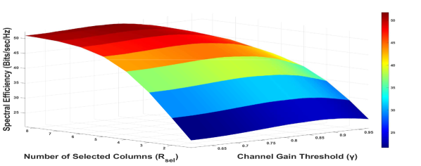
Figure 2: 3D heatmap of SE with respect to selected columns ’$R_{sel}$’ and channel gain threshold, ’$\gamma$’. for IOSVB as will as DR-IOSVB algorithms.

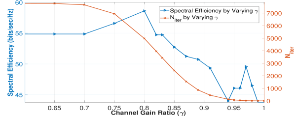
Figure 3: SE and number of iterations ($N_{iter}$) by varying channel gain ratio ($\gamma$).

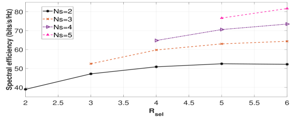
Figure 4: SE for different values of $N_{s}$ by varying $R_{sel}$

IV-B1 Parameter Selection for IOSVB algorithm

Numerical simulations varying $R_{sel}$ and $\gamma$ generated a 3D plot demonstrating SE as a function of these parameters. We run the proposed IOSVB algorithm on 1000 channel realizations and calculate the overall average SE of the MU-MIMO system with $N_{s}=2$. The simulation results are presented in Fig. 2. As $\gamma$ increases, the SE increases to a certain point. This is because higher $\gamma$ values lead to the selection of stronger singular vectors, resulting in increased received signal power. However, increasing $\gamma$ beyond an optimal point reduces the number of candidate singular vectors excessively, limiting the algorithm’s degrees of freedom. Consequently, the algorithm becomes less effective in mitigating inter-user interference, leading to a decline in SE. Furthermore, the figure reveals a positive correlation between the total number of selected beam directions, $R_{sel}$, and SE. Although increasing $R_{sel}$ leads to higher SE, it also results in a simultaneous rise in computational complexity. This is because, for each algorithm realization, $\binom{R_{sel}}{N_{s}}$ combinations must be evaluated to identify the minimum correlated value.

In Fig. 3, we present the SE and the number of iterations by varying the channel gain ratio $\gamma$ for the IOSVB algorithm. The results show that the number of iterations of IOSVB is inversely related to $\gamma$. This arises because as $\gamma$ increases, the number of combinations to be checked decreases. From Fig. 3, we determine the optimal value of $\gamma$ to be approximately $0.80\times\sigma$_max.

To better understand the effect of $R_{sel}$ on SE, we perform numerical simulation by simultaneously varying $N_{s}$ and $R_{sel}$. We use our default MU-MIMO system setup to execute the proposed IOSVB algorithm while sweeping through different values of $N_{s}$ and $R_{sel}$ to calculate the average achieved SE over 1000 channel realizations. The simulation results depicted in Figure 4 reflect that assigning an $R_{sel}$ value of 4 for a data stream $N_{s}=2$ achieves the highest SE with the lowest computational complexity.

Fig. 4 demonstrates that it is unnecessary to increase the value of $R_{sel}$ linearly in relation to the number of data streams, $N_{s}$. We find out the value of $R_{sel}$ for different values of $N_{s}$ that provide 95% SE of the maximum SE. A closer examination of Table IV reveals that the required $R_{sel}$ value does not increase linearly with increasing the value of $N_{s}$. This observation is beneficial, as it helps to mitigate the potential for increased computational complexity at higher $N_{s}$ values.

In fact, we observe that the SVBS algorithm exhibits a similar relationship between $R_{sel}$ and $N_{s}$ as shown in Fig. 4. We also find that the DR-IOSVB algorithm yields nearly identical results concerning algorithmic parameter selection for all the above simulations. This is expected as the DR-IOSVB algorithm follows the same principle as the IOSVB algorithm, with the only difference being the dimensions of the $\bm{F}^{io}$ matrix.

TABLE IV: Required value of $R_{sel}$ for keeping the SE 95% of maximum SE.

Data Streams ($N_{s}$)	Required value of $R_{sel}$
$N_{s}=2$	4
$N_{s}=3$	5
$N_{s}=4$	5
$N_{s}=5$	6

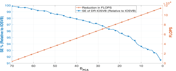
Figure 5: Reduction in computational complexity in terms of FLOPS with S.E of DR-IOSVB compared to IOSVB varying $D_{PCA}$.

IV-B2 Selection of $D_{PCA}$ for DR-IOSVB

To find out the pertinent trade-off between SE and computational cost, we run numerical simulations of the DR-IOSVB algorithm by varying the value $D_{PCA}$ over 1000 channel realizations. It is to be noted that for $D_{PCA}=N_{t}$, the DR-IOSVB is the same as the IOSVB algorithm. In Fig. 5, we present the SE and the decrease in number of floating point operations (FLOPs) for DR-IOSVB with respect to IOSVB by varying $D_{PCA}$. As $D_{PCA}$ reduces, both SE and FLOPS drop compared to IOSVB. However, SE plateaus ( 97%) when $D_{PCA}$ is about 30. This implies any further increase in PCA dimensions beyond 30 offers limited SE benefits relative to added computational overhead. The results highlight the importance of balancing computational effort with SE when choosing $D_{PCA}$ for the algorithm. Note also that Fig. 5 shows the decrease in FLOPs compared to IOSVB, not the actual DR-IOSVB run-time (which is environment-dependent). The greater the FLOP decrease, the greater the computational benefit of DR-IOSVB over IOSVB.

IV-C Performance Analysis

In this subsection, we discuss the simulation results obtained by comparing the performance of the proposed algorithms with other existing algorithms. Below, we briefly describe all the baseline algorithms used in to compare the proposed algorithms.

• Fixed Phase Shifter Alternating Minimization (FPS-AltMin): FPS-AltMin is an algorithm developed for multi-user MIMO systems where it alternates between minimizing the error with respect to the transmitted signals and the phase shifter settings, leveraging fixed phase shifters to balance performance and hardware costs.

• Manifold Optimization Alternating Minimization (MO-AltMin): MO-AltMin is a more complex approach that also employs an alternating minimization strategy in multi-user MIMO systems but utilizes manifold optimization techniques to consider the more realistic case of continuous phase shifters, thus potentially achieving better performance.

• Sub-optimal Algorithm: Here, we denote using the single-user beamforming strategy of selecting the strongest beam directions as described in section II-C in the multi-user case as the sub-optimal algorithm. We also discern that for $\gamma=1$, the IOSVB algorithm reduces to this sub-optimal algorithm.

To evaluate the capability of the proposed algorithms, we conducted a series of Matlab simulations to measure the system’s SE under various conditions, such as different SNR levels and beamforming algorithms.

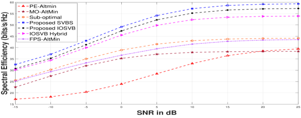
(a) $N_{s}=2$.

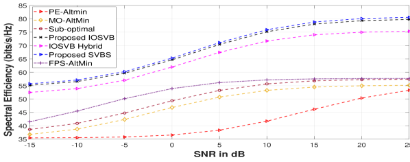
(b) $N_{s}=3$

Figure 6: Comparison between the proposed and existing algorithms in term of SE.

IV-C1 Spectral Efficiency

In Fig. 6, we present the simulation results for a multiple data stream scenario, which compares the achieved SE of the proposed algorithms with other existing beamforming algorithms under different SNR levels. As demonstrated in Fig. 6, the proposed SVBS algorithm delivers the highest SE based on an exhaustive search strategy, albeit with correspondingly high computational complexity. Fig. 6 reveals that the performance of the proposed algorithms improves as the number of data streams increases. For $N_{s}=2$ and $SNR$=15 dB, the proposed IOSVB achieves 31.57% higher SE than the current best FPS-Altmin and a 48.62% improvement compared to MO-AltMin. Fig. 6(b) reveals that the performance of the proposed algorithms improves as the number of data streams increases. For $N_{s}=3$, the proposed IOSVB achieves 38.27% higher SE than FPS-Altmin.

Figure 7: Comparison of SE of various algorithms at different values of $N_{s}$.

To simultaneously compare the performance of all algorithms in multi-data stream scenarios, we set the SNR to a nominal value of 15 dB and highlight the SE averaged over a thousand channel realizations. The results are shown through a bar plot in Fig. 7. We observe that the proposed SVBS algorithm achieves the highest SE for all data streams, closely followed by the proposed IOSVB algorithm.

TABLE V: Computation Time Complexity (in seconds), and Normalized SE (NSE).

Algorithms	$N_{s}$	Time Complexity	NSE
Proposed SVBS	2	388.5931	100%
Proposed IOSVB	2	0.2667	96.53%
IOSVB Hybrid	2	1.4849	91.10%
FPS-AltMin [27]	2	1.4069	72.95%
MO-AltMin [28]	2	13.76	65.17%

IV-C2 Computational Complexity

We compare the computational time required to perform beamforming by the proposed and baseline algorithms. The results are presented in Table V, which provides a comparison of computational time complexity and Normalized SE (NSE) for various algorithms, including the proposed SVBS, IOSVB, IOSVB Hybrid, and several baseline algorithms such as FPS-AltMin, and MO-AltMin. Here, the NSE is calculated by normalizing the SE achieved by each algorithm with the maximum achieved SE (by the SVBS algorithm).

The higher computational complexity of the MO-AltMin algorithm can be attributed to its alternating minimization approach that iteratively optimizes one variable while keeping the others fixed. This methodology requires multiple iterations until convergence, leading to higher computation time.

Meanwhile, the proposed SVBS, although achieving the highest NSE, also exhibits the highest computational time. This can be attributed to the extensive search space and exhaustive search approach utilized, which, while highly effective, demands significant computational resources and time. However, the proposed IOSVB mitigates this by reducing the search space, implementing channel gain thresholding, and introducing an innovative interference-based optimization technique. These improvements dramatically cut the run-time, reducing it from 388.5931 seconds in SVBS to a mere 0.2667 seconds in IOSVB while still maintaining a high NSE of 96.53%.

Additionally, the proposed IOSVB Hybrid algorithm further optimizes the process, striking a balance between computation time and NSE, achieving a reasonably low computation time and an NSE of 91.10%. Still, the computation time is high for the practical application of beamforming. The future BSs will have more computing power, and the computation time will be significantly less. These findings highlight the effectiveness of the proposed approach in different scenarios, emphasizing its practical significance in improving SE and reducing computational complexity. The simulation results provide valuable insights into the performance of the proposed algorithms compared to existing techniques and demonstrate their potential for practical implementation in massive-MIMO multi-user systems.

V Conclusion

Much research has been devoted to MIMO beamforming, particularly on SU-MIMO beamforming. Nevertheless, there is a scarcity of research studies devoted to MU-MIMO beamforming. Furthermore, the SE performance of the current MU-MIMO beamforming approaches falls short of expectations due to ineffective interference management. The notion of correlation of channel singular vector projection for calculating total interference was introduced in this paper. Additionally, beamforming algorithms for MU-MIMO systems were developed by identifying the beams that produce minimal interference. The superior performance and reduced computation times of the proposed algorithms compared to the existing algorithms were empirically illustrated via simulations. The proposed algorithm was run through principal component analysis, which resulted in a substantial decrease in computation time due to the dimension reduction of the channel singular vectors. We additionally developed an exhaustive search algorithm for determining the optimal beamforming vectors, which involves evaluating every singular vector and entails a considerably high computational complexity to establish the upper bound of SE. Regarding SE, we found that the proposed algorithms perform remarkably similarly to the optimal one. Therefore, we firmly hold that the research presented in this paper establishes a novel standard for MU-MIMO beamforming studies in terms of comparing SE and computation time.

From (10) the interference of the fully digital system can be written as,

$$\Delta^{D}_{k}=\sum_{i=1,i\neq k}^{U}|{(\textbf{W}_{k}^{io})}^{H}\textbf{H}_{k}\textbf{F}^{io}|^{2}$$ (38)

.

Corollary 1: If $\textbf{U}_{k}$ is an orthonormal matrix then multiplication of $U_{k}$ and non-square $\textbf{U}_{k}^{H}[\textbf{ind}_{k}]$ results in a sparse matrix, that can be identified as non-square identity matrix,i.e.,

$$\textbf{U}_{k}^{H}[\textbf{ind}_{k}]\;\textbf{U}_{k}=\textbf{I}_{k}[\textbf{ind}_{k}]$$ (39)

where, $\bm{I}_{k}$ is a non square identity matrix.
Proof: Note that $\textbf{U}_{k}$ is a square orthonormal matrix of size $N_{r}\times N_{r}$. As $\textbf{U}_{k}$ is an orthonormal matrix, the multiplication of $\textbf{U}^{H}_{k}$ and $\textbf{U}_{k}$ results in a square identity matrix. Also recall that $\textbf{U}_{k}^{H}[\textbf{ind}_{k}]$ is a matrix of size $N_{s}\times N_{r}$, with each column being an orthonormal vector. Therefore, multiplying rows of $\textbf{U}_{k}^{H}[\textbf{ind}_{k}]$ and columns of $\textbf{U}_{k}$ with the identical index yields ones, whereas multiplying with non-same indexes yields zeroes. Thus, multiplying the matrices of $\textbf{U}_{k}^{H}[\textbf{ind}_{k}]$ and $\textbf{U}_{k}$ yields a non-square identity matrix $\textbf{I}_{k}[\textbf{ind}_{k}]$ of size $N_{s}\times N_{r}$.

Lemma 1: If ’$i$’ is a user interfering and ’$k$’ is the desired user to be transmitted then,

$${||{(\textbf{W}_{k}^{io})}^{H}\textbf{H}_{k}\textbf{F}_{i}^{io}||}^{2}={||\bm{\Sigma}_{k}[\textbf{ind}_{k}]\textbf{V}_{k}^{H}\textbf{V}_{i}[\textbf{ind}_{i}]||}^{2}$$ (40)

Proof: Using (9), we can decompose channel matrix $\textbf{H}_{k}$ into three orthonormal matrices. Hence, we can write

$${||{(\textbf{W}_{k}^{io})}^{H}\textbf{H}_{k}\textbf{F}_{i}^{io}||}^{2}={||{(\textbf{W}_{k}^{io})}^{H}\textbf{U}_{k}\bm{\Sigma}_{k}\textbf{V}_{k}^{H}\textbf{F}_{i}^{io}||}^{2}$$ (41)

Note that, $\textbf{W}_{k}^{io}$ and $\textbf{F}_{k}^{io}$ matrices are found from $\textbf{U}_{k}$ and $\textbf{V}_{k}$ matrices respectively using the corresponding index of selected singular vectors. In other words, it can be written as, $\textbf{U}_{K}[\textbf{ind}_{k}]=\textbf{W}_{k}^{io}$ and $\textbf{V}_{i}[\textbf{ind}_{i}]=\textbf{F}_{k}^{io}$ Hence, (41) can be rewritten as,

$${||{(\textbf{W}_{k}^{io})}^{H}\textbf{H}_{k}\textbf{F}_{i}^{io}||}^{2}={||\textbf{U}_{k}^{H}[\textbf{ind}_{k}]\textbf{U}_{k}\bm{\Sigma}_{k}\textbf{V}_{k}^{H}\textbf{V}_{i}[\textbf{ind}_{i}]||}^{2}$$ (42)

Now, using Corollary 1, we can write,

$${||{(\textbf{W}_{k}^{io})}^{H}\textbf{H}_{k}\textbf{F}_{i}^{io}||}^{2}={||\textbf{I}_{k}[\textbf{ind}_{k}]\mathbf{\Sigma}_{k}\textbf{V}_{k}^{H}\textbf{V}_{i}[\textbf{ind}_{i}]||}^{2}$$ (43)

Here, $\textbf{I}_{k}[\textbf{ind}_{k}]$ is a non-square identity matrix with $N_{s}$ non-zero entries. Using matrix multiplication, (43) can be written as

$${||{(\textbf{W}_{k}^{io})}^{H}\textbf{H}_{k}\textbf{F}_{i}^{io}||}^{2}={||\mathbf{\Sigma}_{k}[\textbf{ind}_{k}]\textbf{V}_{k}^{H}\textbf{V}_{i}[\textbf{ind}_{i}]||}^{2}$$ (44)

Lemma 2: If A and B are two matrices, and $\textbf{A}=\begin{bmatrix}x_{1}\cdots x_{k}\cdots x_{U}\end{bmatrix}^{T}$ and $\textbf{B}=\begin{bmatrix}y_{1}\cdots y_{i}\cdots y_{U}\end{bmatrix}$

then,

Proof: Consider A is a $3\times 1$ matrix and B is a $1\times 3$ matrix. Then multiplication of A and B results in as follows,

$$\textbf{A}.\textbf{B}=\begin{bmatrix}x_{1}\\ x_{2}\\ x_{3}\end{bmatrix}.{\begin{bmatrix}y_{1}&y_{2}&y_{3}\end{bmatrix}}=\begin{bmatrix}x1.y1&x1.y2&x1.y3\\ x2.y1&x2.y2&x2.y3\\ x3.y1&x3.y2&x3.y3\end{bmatrix}$$ (45)

Now, if the row index of the matrix A is denoted as $i$, and the column index of the matrix B is denoted as k, and we add a condition $i\neq k$ in the multiplication of equation then it can be rewritten as,

$$\begin{bmatrix}x_{1}\\ x_{2}\\ x_{3}\end{bmatrix}.{{\begin{bmatrix}y_{1}&y_{2}&y_{3}\end{bmatrix}}}_{i\neq k}=\begin{bmatrix}0&x1.y2&x1.y3\\ x2.y1&0&x2.y3\\ x3.y1&x3.y2&0\end{bmatrix}$$ (46)

As the preceding equation makes clear, adding the constraint $i\neq k$ eliminates the diagonal components from the product of A and B, so we can write

$${\begin{bmatrix}x_{1}\\ x_{2}\\ x_{3}\end{bmatrix}}.{{\begin{bmatrix}y_{1}&y_{2}&y_{3}\end{bmatrix}}}_{i\neq k}=\textbf{A}.\textbf{B}-diag(\textbf{A}.\textbf{B})$$ (47)

Theorem: If the total interference over all users is expressed as $I_{t}$, in other words, $\sum_{k=1}^{U}\Delta^{D}_{k}=I_{t}$, then the interference ${I_{t}}$ can be written as,

$$I_{t}=\sum_{k=1}^{U}\sum_{i=1;i\neq k}^{U}{||{(\textbf{W}_{k}^{io})}^{H}\textbf{H}_{k}\textbf{F}_{i}^{io}||}^{2}={||\textbf{C}_{corr}^{i}-diag(\textbf{C}_{corr}^{i})||}^{2}$$ (48)

Here, $\textbf{C}_{corr}^{i}={(\textbf{F}^{sel}[\textbf{ind}]\mathbf{\Sigma}[\textbf{ind}])}^{H}\textbf{F}^{sel}[\textbf{ind}]$ is the correlation matrix of the system.

Proof: Using Lemma 1, we can write,

$$I_{t} =\sum_{k=1}^{U}\sum_{i=1;i\neq k}^{U}{||{(\textbf{W}_{k}^{io})}^{H}\textbf{H}_{k}\textbf{F}_{i}^{io}||}^{2}$$

$$=\sum_{k=1}^{U}\sum_{i=1;i\neq k}^{U}{||\mathbf{\Sigma}_{k}[\textbf{ind}_{k}]\textbf{V}_{k}^{H}\textbf{V}_{i}[\textbf{ind}_{i}]||}^{2}$$ (49)

By concatenating the $\textbf{V}_{i}$ matrix by removing the inner summation, (49) can further be written as

$${I_{t}=\sum_{k=1}^{U}{||\mathbf{\Sigma}_{k}[\textbf{ind}_{k}]\textbf{V}_{k}^{H}\;{[\textbf{V}_{1}{[\textbf{ind}_{1}]}\cdots\textbf{V}_{i}{[\textbf{ind}_{i}]}\cdots{\textbf{V}_{U}}{[\textbf{ind}_{U}]}]}_{i\neq k}||}^{2}}$$ (50)

Now, removing the remaining summation, (50) can be expressed as

$${I_{t}=\left\lVert\begin{bmatrix}\mathbf{\Sigma}_{1}[\textbf{ind}_{1}]\textbf{V}_{1}^{H}\\ .\\ .\\ \mathbf{\Sigma}_{k}[\textbf{ind}_{k}]\textbf{V}_{k}^{H}\\ .\\ .\\ \mathbf{\Sigma}_{U}[\textbf{ind}_{U}]\textbf{V}_{U}^{H}\end{bmatrix}{\begin{bmatrix}\textbf{V}_{1}[\textbf{ind}_{1}]\cdots\textbf{V}_{i}[\textbf{ind}_{i}]\cdots\textbf{V}_{U}[\textbf{ind}_{U}]\end{bmatrix}}_{i\neq k}\right\rVert^{2}}$$ (51)

Using Lemma 2, (51) can be further simplified as,

References

- [1] L. Lu, G. Y. Li, A. L. Swindlehurst, A. Ashikhmin, and R. Zhang, “An overview of massive mimo: Benefits and challenges,” IEEE journal of selected topics in signal processing, vol. 8, no. 5, pp. 742–758, 2014.
- [2] T. L. Marzetta and H. Yang, Fundamentals of massive MIMO. Cambridge University Press, 2016.
- [3] T. L. Marzetta, “Noncooperative cellular wireless with unlimited numbers of base station antennas,” IEEE transactions on wireless communications, vol. 9, no. 11, pp. 3590–3600, 2010.
- [4] D. Gesbert, S. Hanly, H. Huang, S. S. Shitz, O. Simeone, and W. Yu, “Multi-cell mimo cooperative networks: A new look at interference,” IEEE J.Sel. A. Commun., vol. 28, no. 9, p. 1380–1408, dec 2010. [Online]. Available: https://doi.org/10.1109/JSAC.2010.101202
- [5] E. G. Larsson, O. Edfors, F. Tufvesson, and T. L. Marzetta, “Massive mimo for next generation wireless systems,” IEEE Communications Magazine, vol. 52, no. 2, pp. 186–195, 2014.
- [6] R. Chataut and R. Akl, “Massive mimo systems for 5g and beyond networks—overview, recent trends, challenges, and future research direction,” Sensors, vol. 20, no. 10, 2020. [Online]. Available: https://www.mdpi.com/1424-8220/20/10/2753
- [7] E. Björnson, R. Zakhour, D. Gesbert, and B. Ottersten, “Cooperative multicell precoding: Rate region characterization and distributed strategies with instantaneous and statistical csi,” IEEE Transactions on Signal Processing, vol. 58, no. 8, pp. 4298–4310, 2010.
- [8] L. Dai, X. Gao, J. Quan, S. Han, and I. Chih-Lin, “Near-optimal hybrid analog and digital precoding for downlink mmwave massive mimo systems,” in 2015 IEEE International Conference on Communications (ICC). IEEE, 2015, pp. 1334–1339.
- [9] A. Adhikary, J. Nam, J.-Y. Ahn, and G. Caire, “Joint spatial division and multiplexing—the large-scale array regime,” IEEE transactions on information theory, vol. 59, no. 10, pp. 6441–6463, 2013.
- [10] Q. Li, G. Li, W. Lee, M.-i. Lee, D. Mazzarese, B. Clerckx, and Z. Li, “Mimo techniques in wimax and lte: a feature overview,” IEEE Communications magazine, vol. 48, no. 5, pp. 86–92, 2010.
- [11] S.-H. Park, O. Simeone, O. Sahin, and S. Shamai, “Joint precoding and multivariate backhaul compression for the downlink of cloud radio access networks,” IEEE Transactions on Signal Processing, vol. 61, no. 22, pp. 5646–5658, 2013.
- [12] J. Jing, C. Xiaoxue, and X. Yongbin, “Energy-efficiency based downlink multi-user hybrid beamforming for millimeter wave massive mimo system,” The Journal of China Universities of Posts and Telecommunications, vol. 23, no. 4, pp. 53–62, 2016.
- [13] I. Ahmed, H. Khammari, and A. Shahid, “Resource allocation for transmit hybrid beamforming in decoupled millimeter wave multiuser-mimo downlink,” IEEE Access, vol. 5, pp. 170–182, 2016.
- [14] A. Garcia-Rodriguez, V. Venkateswaran, P. Rulikowski, and C. Masouros, “Hybrid analog–digital precoding revisited under realistic rf modeling,” IEEE Wireless Communications Letters, vol. 5, no. 5, pp. 528–531, 2016.
- [15] D. H. Nguyen, L. B. Le, and T. Le-Ngoc, “Hybrid mmse precoding for mmwave multiuser mimo systems,” in 2016 IEEE international conference on communications (ICC). IEEE, 2016, pp. 1–6.
- [16] M. S. Ullah, S. C. Sarker, Z. B. Ashraf, and M. F. Uddin, “Spectral efficiency of multiuser massive mimo-ofdm thz wireless systems with hybrid beamforming under inter-carrier interference,” in 2022 12th International Conference on Electrical and Computer Engineering (ICECE). IEEE, 2022, pp. 228–231.
- [17] D. Ying, F. W. Vook, T. A. Thomas, and D. J. Love, “Hybrid structure in massive mimo: Achieving large sum rate with fewer rf chains,” in 2015 IEEE International Conference on Communications (ICC). IEEE, 2015, pp. 2344–2349.
- [18] J. Cai, B. Rong, and S. Sun, “A low complexity hybrid precoding scheme for massive mimo system,” in 2016 16th international symposium on communications and information technologies (ISCIT). IEEE, 2016, pp. 638–641.
- [19] S. Fujio, C. Kojima, T. Shimura, K. Nishikawa, K. Ozaki, Z. Li, A. Honda, S. Ishikawa, T. Ohshima, H. Ashida et al., “Robust beamforming method for sdma with interleaved subarray hybrid beamforming,” in 2016 IEEE 27th Annual International Symposium on Personal, Indoor, and Mobile Radio Communications (PIMRC). IEEE, 2016, pp. 1–5.
- [20] L. Liang, W. Xu, and X. Dong, “Low-complexity hybrid precoding in massive multiuser mimo systems,” IEEE Wireless Communications Letters, vol. 3, no. 6, pp. 653–656, 2014.
- [21] J. Zhang, A. Wiesel, and M. Haardt, “Low rank approximation based hybrid precoding schemes for multi-carrier single-user massive mimo systems,” in 2016 IEEE International Conference on Acoustics, Speech and Signal Processing (ICASSP). IEEE, 2016, pp. 3281–3285.
- [22] J. Brady, N. Behdad, and A. M. Sayeed, “Beamspace mimo for millimeter-wave communications: System architecture, modeling, analysis, and measurements,” IEEE Transactions on Antennas and Propagation, vol. 61, no. 7, pp. 3814–3827, 2013.
- [23] Z. C. Phyo and A. Taparugssanagorn, “Hybrid analog-digital downlink beamforming for massive mimo system with uniform and non-uniform linear arrays,” in 2016 13th International Conference on Electrical Engineering/Electronics, Computer, Telecommunications and Information Technology (ECTI-CON). IEEE, 2016, pp. 1–6.
- [24] G. Kwon, Y. Shim, H. Park, and H. M. Kwon, “Design of millimeter wave hybrid beamforming systems,” in 2014 IEEE 80th Vehicular Technology Conference (VTC2014-Fall). IEEE, 2014, pp. 1–5.
- [25] A. Alkhateeb, O. El Ayach, G. Leus, and R. W. Heath, “Hybrid precoding for millimeter wave cellular systems with partial channel knowledge,” in 2013 Information Theory and Applications Workshop (ITA). IEEE, 2013, pp. 1–5.
- [26] O. El Ayach, S. Rajagopal, S. Abu-Surra, Z. Pi, and R. W. Heath, “Spatially sparse precoding in millimeter wave mimo systems,” IEEE transactions on wireless communications, vol. 13, no. 3, pp. 1499–1513, 2014.
- [27] X. Yu, J. Zhang, and K. B. Letaief, “Hybrid precoding in millimeter wave systems: How many phase shifters are needed?” in GLOBECOM 2017-2017 IEEE Global Communications Conference. IEEE, 2017, pp. 1–6.
- [28] X. Yu, J.-C. Shen, J. Zhang, and K. B. Letaief, “Alternating minimization algorithms for hybrid precoding in millimeter wave mimo systems,” IEEE Journal of Selected Topics in Signal Processing, vol. 10, no. 3, pp. 485–500, 2016.
- [29] Z. Gao, C. Hu, L. Dai, and Z. Wang, “Channel estimation for millimeter-wave massive mimo with hybrid precoding over frequency-selective fading channels,” IEEE Communications Letters, vol. 20, no. 6, pp. 1259–1262, 2016.
- [30] F. Sohrabi and W. Yu, “Hybrid digital and analog beamforming design for large-scale antenna arrays,” IEEE Journal of Selected Topics in Signal Processing, vol. 10, no. 3, pp. 501–513, 2016.
- [31] A. Liu and V. K. Lau, “Impact of csi knowledge on the codebook-based hybrid beamforming in massive mimo,” IEEE Transactions on Signal Processing, vol. 64, no. 24, pp. 6545–6556, 2016.
- [32] R. Zi, X. Ge, J. Thompson, C.-X. Wang, H. Wang, and T. Han, “Energy efficiency optimization of 5g radio frequency chain systems,” IEEE Journal on Selected Areas in Communications, vol. 34, no. 4, pp. 758–771, 2016.
- [33] A. Alkhateeb and R. W. Heath, “Frequency selective hybrid precoding for limited feedback millimeter wave systems,” IEEE Transactions on Communications, vol. 64, no. 5, pp. 1801–1818, 2016.
- [34] H. Yuan et al., “Hybrid beamforming for terahertz multi-carrier systems over frequency selective fading,” IEEE Transactions on Communications, vol. 68, no. 10, pp. 6186–6199, 2020.
- [35] Q. H. Spencer, B. D. Jeffs, M. A. Jensen, and A. L. Swindlehurst, “Modeling the statistical time and angle of arrival characteristics of an indoor multipath channel,” IEEE Journal on Selected areas in communications, vol. 18, no. 3, pp. 347–360, 2000.
- [36] C. Lin and G. Y. Li, “Indoor terahertz communications: How many antenna arrays are needed?” IEEE Transactions on Wireless Communications, vol. 14, no. 6, pp. 3097–3107, 2015.
- [37] T. S. Rappaport, R. W. Heath Jr, R. C. Daniels, and J. N. Murdock, Millimeter wave wireless communications. Pearson Education, 2015.
- [38] C. Lin and G. Y. Li, “Indoor terahertz communications: How many antenna arrays are needed?” IEEE Transactions on Wireless Communications, vol. 14, no. 6, pp. 3097–3107, 2015.
- [39] H. Kasai, “Fast optimization algorithm on complex oblique manifold for hybrid precoding in millimeter wave mimo systems,” in 2018 IEEE Global Conference on Signal and Information Processing (GlobalSIP). IEEE, 2018, pp. 1266–1270.
- [40] R. U. Murshed, Z. B. Ashraf, A. H. Hridhon, K. Munasinghe, A. Jamalipour, and M. F. Hossain, “A cnn-lstm-based fusion separation deep neural network for 6g ultra-massive mimo hybrid beamforming,” IEEE Access, vol. 11, pp. 38 614–38 630, 2023.
- [41] A. Alkhateeb, G. Leus, and R. W. Heath, “Limited feedback hybrid precoding for multi-user millimeter wave systems,” IEEE transactions on wireless communications, vol. 14, no. 11, pp. 6481–6494, 2015.
- [42] H. Yuan, N. Yang, K. Yang, C. Han, and J. An, “Hybrid beamforming for mimo-ofdm terahertz wireless systems over frequency selective channels,” in 2018 IEEE Global Communications Conference (GLOBECOM). IEEE, 2018, pp. 1–6.
- [43] J. Zhang, X. Yu, and K. B. Letaief, “Hybrid beamforming for 5g and beyond millimeter-wave systems: A holistic view,” IEEE Open Journal of the Communications Society, vol. 1, pp. 77–91, 2019.
- [44] R. Li, B. Guo, M. Tao, Y.-F. Liu, and W. Yu, “Joint design of hybrid beamforming and reflection coefficients in ris-aided mmwave mimo systems,” IEEE Transactions on Communications, vol. 70, no. 4, pp. 2404–2416, 2022.
- [45] T. Lin, J. Cong, Y. Zhu, J. Zhang, and K. B. Letaief, “Hybrid beamforming for millimeter wave systems using the mmse criterion,” IEEE Transactions on Communications, vol. 67, no. 5, pp. 3693–3708, 2019.
- [46] Y. Shi, J. Zhang, and K. B. Letaief, “Low-rank matrix completion via riemannian pursuit for topological interference management,” in 2015 IEEE International Symposium on Information Theory (ISIT). IEEE, 2015, pp. 1831–1835.
- [47] R. U. Murshed, A. Horaira Hridhon, and M. F. Hossain, “Deep learning based power allocation in 6g urllc for jointly optimizing latency and reliability,” in 2021 5th International Conference on Electrical Information and Communication Technology (EICT), 2021, pp. 1–6.