Refining resource estimation for the quantum computation of vibrational molecular spectra through Trotter error analysis

Abstract

Accurate simulations of vibrational molecular spectra are expensive on conventional computers. Compared to the electronic structure problem, the vibrational structure problem with quantum computers is less investigated. In this work we accurately estimate quantum resources, such as number of qubits and quantum gates, required for vibrational structure calculations on a programmable quantum computer. Our approach is based on quantum phase estimation and focuses on fault-tolerant quantum devices. In addition to asymptotic estimates for generic chemical compounds, we present a more detailed analysis of the quantum resources needed for the simulation of the Hamiltonian arising in the vibrational structure calculation of acetylene-like polyynes of interest. Leveraging nested commutators, we provide an in-depth quantitative analysis of trotter errors compared to the prior investigations. Ultimately, this work serves as a guide for analyzing the potential quantum advantage within vibrational structure simulations.

1 Introduction

Attaining the electronic structure of molecules is one of the core problems in quantum chemistry and material design [30]. Although the electronic structure of small molecules can be obtained with good accuracy, solving the electronic structure of larger molecular systems continues to be challenging and computationally intensive. A vast number of methods – such as Hartree-Fock, configuration interaction, coupled cluster theory, and density functional theory – have been developed to address the accuracy and efficiency in treating the molecular electronic-structure problems [17, 24, 12, 19]. Quantum computing, on the other hand, offers an alternative approach to tackle the computational challenges associated with these problems using quantum hardware [3, 27, 7]. Significant advances have been made in the past two decades in the development of quantum algorithms to harness the capabilities of currently available noisy quantum devices, particularly for addressing electronic-structure problems [23, 20, 34, 8]. Additionally, researchers have also estimated the quantum resources required for simulating molecular electronic structure on future fault-tolerant quantum devices [35].

In the realm of modern chemistry, electronic structure calculations play a crucial role in obtaining structural properties and spectroscopic characteristics of molecules, as descriptors enabling screening of materials in industrial applications. However, the quest for accurate and efficient electronic structure methods is not the sole computational obstacle in quantum chemistry and material science. The vibrational structure problem represents another fundamental challenge. To make a palpable impact in both fundamental science and industrial applications, it becomes necessary to delve beyond the electronic structure and construct a kinetic model that requires comprehensive understanding of the molecular vibrational structure, e.g., to determine reaction rate constants [22, 41]. While classical computers can handle the electronic structure problem of small molecules with reasonable accuracy, the same does not hold true for calculating the vibrational structure of molecules beyond the harmonic approximation. Previous works suggest that quantum-computing approaches for calculating vibrational structure have the potential to reach quantum advantage prior to their electronic-structure counterparts, for the respective required energy precision [39]. Nevertheless, the quantum computing applications for molecular vibrational structure calculations have received limited scholarly attention. Only a modest number of studies have been conducted to date, and these studies marginally address the quantum resource requirements [39, 38, 37, 33, 40, 28, 29, 18, 36, 14]. The authors in [39] present algorithms for calculating vibrational spectra on both near- and long-term quantum devices. They compare concrete quantum resources such as qubit count, as well as proxy quantities determining computational complexity, e.g. Hamiltonian magnitude, for both electronic and vibrational structure simulations. Lastly, they present numerical error analyses on several vibrational Hamiltonian examples - carbon monoxide, the isoformyl radical, ozone, and a model Hamiltonian of Fermi resonance - as a proof of principle. They speculate quantum advantage will take place for a real-world vibrational structure problem instance before any electronic structure one. However, they suggest further investigation on correlation between vibrational problem instances and Trotter error.

Here, we present a more extensive study of the Trotter error for vibrational structure simulations based on the recent theory in ref. [10]. Our focus in this work is on providing quantum resource estimation for simulating molecular vibrational structure. To improve the previous studies, we start with a distinct Hamiltonian model to go beyond harmonic approximation and obtain precise Hamiltonians for the examples represented in this work. Our results are based on the “$L$-mode representation” of the Hamiltonian and the vibrational self-consistent field (VSCF) method [16]. We first offer an asymptotic analysis and then provide a more quantitative study on industrially-relevant chemical compounds. More specifically, our focus in the examples here is on polyyne molecules, which are the dominant intermediates in the commercial upgrade of light gases to the more attractive carbon nano-tubes and carbon-fiber materials.

In the next section we will introduce a quantum approach for vibrational structure calculations and analyze its computational complexity. As mentioned above, our study here is based on the $L$-mode Hamiltonian representation which is more suitable for asymptotic analysis. We review mapping of the vibrational Hamiltonian to qubits and present comparison of qubit requirements for the “unary” and “binary” encoding methods. Note that throughout this article the term “qubit” refers to “logical qubits” and we will not discuss any specific error-correction methods. We continue Section 2 by estimating the complexity of the algorithm (based on quantum phase estimation) when Trotterization is used for approximate Hamiltonian evolution. In Section 3, we focus on improving the accuracy of our asymptotic studies, following up on the results from Childs et al. [10]. In Section 4, we deliver more precise numerical results on the quantum computational cost for a set of industrially-relevant chemical compounds, namely acetylene-like polyyne molecules. Finally, we provide a summary of our results, and discuss the themes for future research in comparing the quantum resource requirements for vibrational and electronic structure problems.

2 Quantum algorithm for vibrational structure calculations

Like other quantum algorithms, as illustrated in the diagram above, a quantum algorithm for vibrational structure problems is consisted of several distinct steps. In the following subsections, we will delve into these steps in detail, tying everything together to provide asymptotic resource estimates in section 2.4. We should note that a pivotal aspect of Hamiltonian simulation involves determining the parameters, such as the number of Trotter steps, to yield results sufficeintly accurate for the application at hand. This may necessitate some preprocessing of the qubit Hamiltonian terms (falling between the second and third steps of the diagram). We will discuss this further in section 3.

2.1 The vibrational Hamiltonian

A general expression for the vibrational Hamiltonian is given by the multi-mode expansion, called $L$-mode representation, which expands the potential energy surface into a sum of one-mode potentials, two-mode potentials, three-mode potentials, and so on [5, 26]. The Hamiltonian for a system with $L$ modes of vibration each denoted by a variable $Q_{.}$ is given as:

$$\mathcal{H}_{\textrm{v}ib}(Q_{1},\ldots,Q_{L}) =-\frac{1}{2}\sum_{l=1}^{L}\frac{\partial^{2}}{\partial Q_{l}^{2}}+V(Q_{1},\ldots,Q_{L})$$

$$V(Q_{1},\ldots,Q_{L}) =V_{0}+\sum_{l=1}^{L}V^{[l]}(Q_{l})+\sum_{l<m}^{L}V^{[l,m]}(Q_{l},Q_{m})$$

$$+\sum_{l<m<n}^{L}V^{[l,m,n]}(Q_{l},Q_{m},Q_{n})+\dots$$

The Hamiltonian expansion is truncated at arbitrary order $D$ which can take integer values up to $L$. We also assume that the maximum occupation number of each bosonic mode is truncated to order $d$. The second quantization is introduced through a general set of one-particle basis functions called modals. To each mode, $l$, is then associated a number $d$ of modals $\{\phi_{n_{l}}\}$. The Hamiltonian becomes

$$\mathcal{H}_{\textrm{v}ib}^{SQ}= \sum_{l=1}^{L}\sum_{k,h}^{d}\left\langle\phi_{k_{l}}\right|T(Q_{l})+V^{[l]}(Q_{l})\left|\phi_{h_{l}}\right\rangle a_{k_{l}}^{\dagger}a_{h_{l}}$$ (1)

$$+ \sum_{l<m}^{L}\sum_{k,h}^{d}\sum_{k,h}^{d}\left\langle\phi_{k_{l}}\phi_{k_{m}}\right|V^{[l,m]}(Q_{l},Q_{m})\left|\phi_{h_{l}}\phi_{h_{m}}\right\rangle a_{k_{l}}^{\dagger}a_{k_{m}}^{\dagger}a_{h_{l}}a_{h_{m}}+\dots$$

where $a_{\cdot}^{\dagger}$ and $a_{\cdot}$ are the creation and annihilation operators, respectively, discussed below. The number of terms in the Hamiltonian then amounts to

$$N_{H}={\mathcal{O}}((Ld^{2})^{D})\,.$$ (2)

Table 1: Table of variables used in this work and their corresponding meaning

Symbol	Meaning
$D$	Truncation order of the Hamiltonian expansion
$d$	Truncation order of the bosonic modes occupation (i.e. number of modals)
$L$	Number of modes
$p$	Order of the Trotter expansion

The various truncation orders and other fundamental sizing parameters are summarized in table 1.

Note that in practice, there are two approaches commonly employed to obtain modals and construct the system Hamiltonian: the VSCF method and the Harmonic approximation. In this work, we use VSCF method based on second quantization [16, 13] and our focus will be on the anharmonic vibrational wave function, see Appendix A for more details.

2.2 Qubit encodings

Quantum operators in the Hamiltonian (1) act on indistinguishable bosons, which need to be mapped onto distinguishable qubits. Qubit encoding facilitates this mapping by transforming the bosonic Fock space into the qubit Hilbert space, where each bosonic state is represented by a corresponding qubit state. In this section, we provide a comparison between unary and binary encodings, see ref. [38] for example. Specifically, we focus our discussion on the standard binary encoding. It is important to note that there is an exponential number of ways to encode $d$ integers in $\log_{2}(d)$ bits allowing for the existence of alternative binary encoding methods. One such example is the Gray code, which ensures the binary representations of neighboring integers have a Hamming distance of one. In practice, the choice of mapping can be customized and optimized according to the specific system of interest.

With the unary encoding, the many-body basis functions $\phi_{k_{1}}\cdots\phi_{k_{L}}$ can be encoded as an occupation number vector (ONV) as

$$\phi_{k_{1}}\cdots\phi_{k_{L}}:=\left|0_{1}\cdots 1_{k_{1}}\cdots 0_{d},\cdots,0_{1}\cdots 1_{k_{L}}\cdots 0_{d}\right\rangle\,.$$ (3)

Based on this representation, the creation and annihilation operators act on modal $k_{l}$ of mode $l$ as:

$$a_{k_{l}}^{\dagger}\left|\cdots,0_{1}\cdots 0_{k_{l}}\cdots 0_{d},\cdots\right\rangle =\left|\cdots,0_{1}\cdots 1_{k_{l}}\cdots 0_{d},\cdots\right\rangle$$ (4)

$$a_{k_{l}}^{\dagger}\left|\cdots,0_{1}\cdots 1_{k_{l}}\cdots 0_{d},\cdots\right\rangle =0$$

$$a_{k_{l}}\left|\cdots,0_{1}\cdots 1_{k_{l}}\cdots 0_{d},\cdots\right\rangle =\left|\cdots,0_{1}\cdots 0_{k_{l}}\cdots 0_{d},\cdots\right\rangle$$

$$a_{k_{l}}\left|\cdots,0_{1}\cdots 0_{k_{l}}\cdots 0_{d},\cdots\right\rangle =0$$

with

$$\left[a_{k_{l}}^{\dagger},a_{h_{m}}^{\dagger}\right] =0\,,\quad\left[a_{k_{l}},a_{h_{m}}\right] =0\,,\,\,\text{and}\quad\left[a_{k_{l}},a_{h_{m}}^{\dagger}\right] =\delta_{l,m}\,,\delta_{k_{l},h_{m}}\,.$$ (5)

Therefore the mapping to Pauli operators is straightforward:

$$a^{\dagger}_{k_{l}}=\sigma^{x}_{k_{l}}-i\sigma^{y}_{k_{l}}\,,\quad\text{and}\qquad a_{k_{l}}=\sigma^{x}_{k_{l}}+i\sigma^{y}_{k_{l}}\,.$$ (6)

In the case of a binary mapping, the situation is different. Any operator acting on a $d$-level system can be written as:

$$\mathcal{A}=\sum_{l,l^{\prime}}c_{l,l^{\prime}}|l\rangle\langle l^{\prime}|\,,$$ (7)

where $\left|l\right\rangle$ is a $\log_{2}(d)$-long bitstring encoding the binary representation of the integer $l$. Each term can be rewritten in terms of the tensor product of individual qubit states $\left|l\right\rangle\left\langle l^{\prime}\right|=\bigotimes_{j}\left|x_{j}\right\rangle\left\langle x_{j}^{\prime}\right|$. To map the bosonic operators $a^{\dagger}_{k_{l}}$ and $a_{k_{l}}$ to Pauli operators, one first has to translate the products $a^{\dagger}_{k_{l}}a_{h_{l}}$, $a^{\dagger}_{k_{l}}a^{\dagger}_{k_{m}}a_{h_{l}}a_{h_{m}}$, etc, to operators of the form of Eq. (7). For instance, consider now the ONV to be $\left|k_{1},\cdots,k_{L}\right\rangle$ with each $\left|k_{l}\right\rangle$ the binary representation of integer $k_{l}$. Then a one-body product can be written as

$$a^{\dagger}_{k_{l}}a_{h_{l}}=\left|\cdots,k_{l},\cdots\right\rangle\left\langle\cdots,h_{l},\cdots\right|\,.$$ (8)

Then the following formulae can be employed,

$$\left|0\right\rangle\left\langle 1\right|=\frac{1}{2}(\sigma^{x}+i\sigma^{y})\,,\quad\left|1\right\rangle\left\langle 0\right|=\frac{1}{2}(\sigma^{x}-i\sigma^{y})\,,$$ (9)

$$\left|0\right\rangle\left\langle 0\right|=\frac{1}{2}(I+\sigma^{z})\,,\qquad\left|1\right\rangle\left\langle 1\right|=\frac{1}{2}(I-\sigma^{z})\,.$$

The unary encoding requires a total number of qubits $N_{q}=Ld$ whereas any binary encoding leads to $N_{q}=L\log_{2}(d)$. After mapping, the number of Pauli terms in the unary Hamiltonian is given by the number of terms in the second quantized Hamiltonian only, as the unary mapping leads to a constant number of Paulis per term. On the other hand, the binary encoding leads to a total number of Pauli terms scaling as ${\mathcal{O}}(N_{H}\log_{2}(d))$. For the unary encoding the Pauli terms are $2D$-local, meaning that, at maximum order, they act non-trivially on $2D$ qubits at a time. In contrast, the binary encoding leads to operators acting on ${\mathcal{O}}(2D\log_{2}(d))$ qubits. Note that this is an upper bound as in principle the encoding can be optimized so that terms involving strings with large Hamming distance are associated to negligible Hamiltonian coefficients. The choice of the number of modals $d$ is application specific and is generally determined by the temperature at which the property of interest is studied. For the polyyne molecules that we will discuss in Section 4, $d$ is small and hence unary and binary mapping for total number of Pauli terms and locality of Pauli terms are comparable. As we will explore further, in most applications, $D=3$ proves to be a satisfactory choice for vibrational structure problems, resulting in highly local Pauli terms in the Hamiltonian in comparison to the fermionic case. Indeed, mapping fermionic to qubit Hamiltonians in electronic structure simulations requires tracking the parity of the occupation numbers of orbitals in order to satisfy anti-commutation relations of the fermionic operators. This leads to creation of Pauli operators that have a locality of ${\mathcal{O}}(N)$ where $N$ is the number of qubits required to represent a $N$ spin-orbital system [6] for e.g. Jordan-Wigner mapping. While there exist other fermion to qubit mappings that are ${\mathcal{O}}(\log(N))$ local like the Bravyi-Kitaev mapping, we focus on the Jordan-Wigner mapping for comparison in this discussion as it is more widely used than the other mappings.

2.3 Quantum Phase Estimation

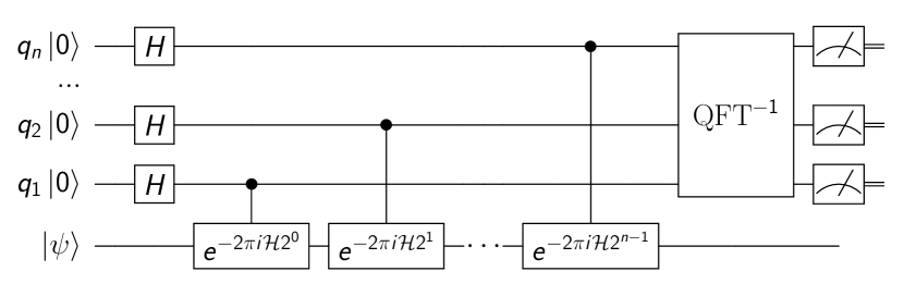
Figure 1: The canonical implementation of the QPE algorithm in a quantum circuit

Eigenvalues of a given Hamiltonian, $\mathcal{H}$, can be evaluated with the quantum phase estimation (QPE) algorithm. The canonical implementation of this algorithm in a quantum circuit is given in Figure 1. First an eigenstate , $\left|\psi\right\rangle$, corresponding to eigenvalue $\lambda$, is prepared in the quantum register. An ancilla register of $n$ qubits is initialized in full superposition state. Then $\left|\psi\right\rangle$ is evolved under powers of $\exp(-2\pi i\mathcal{H})$. The evolution operators are controlled by the ancilla qubits as shown in Figure 1. At this point the state in the quantum register is

$$\left|\psi^{\prime}\right\rangle=\frac{1}{2^{\frac{n}{2}}}\sum_{x=0}^{2^{n}}e^{-2\pi i\lambda x}\left|x\right\rangle.$$ (10)

Assuming $\lambda$ belongs to [0,1], it can be approximated by $\gamma=y/2^{n}$, with $y$ being an integer. The inverse quantum Fourier transform (QFT) then kicks back the phase to the state of the ancilla register. If $\lambda=\gamma$, the inverse QFT leaves the ancilla register in the product state $\left|y\right\rangle$ which is then read with $100\%$ probability of success. However, in the more general case where $|\lambda-\gamma|>0$, $\lambda$ can be obtained with $k$ correct digits and probability of at least 0.75 if the number of ancilla qubits is $n=k+\log_{2}(4)=k+2$ [32, Eqn. (5.35)].

To enforce the assumption that the eigenvalue is in $[0,1]$, QPE is applied to a shifted and scaled Hamiltonian $\tilde{\mathcal{H}}$ with spectrum contained in $[0,1]$: $\tilde{\mathcal{H}}=\frac{1}{2\beta}(\mathcal{H}+\beta I)$, where $[-\beta,\beta]$ contains the spectrum of $\mathcal{H}$. Usually, $\beta$ is simply taken to be the norm of the Hamiltonian $\beta=\left\|\mathcal{H}\right\|$. In particular, when the Hamiltonian is a weighted sum of Pauli operators such that $\mathcal{H}=\sum_{i}c_{i}\mathcal{P}_{i}$, then $\left\|\mathcal{H}\right\|=\sum_{i}|c_{i}|$. We call $\epsilon_{\nu}$ the targeted spectroscopic accuracy of our calculations. In practice, for vibrational structure problems, $\epsilon_{\nu}$ is often set to $1~{}\text{cm}^{-1}$. If QPE evaluates the eigenvalue of the scaled Hamiltonian with precision $2^{-k}$, then we set $k=\left\lceil\log_{2}(2\beta\epsilon_{\nu}^{-1})\right\rceil$ to achieve the desired accuracy. Combining these requirements, the number of ancilla qubits required in the QPE to read the eigenvalue with precision $\epsilon_{\nu}$ and probability of at least 0.75 is given by $n=\left\lceil\log_{2}(8\beta\epsilon_{\nu}^{-1})\right\rceil$.

2.4 Hamiltonian evolution and total gate complexity

Executing QPE requires implementing a quantum circuit to perform the (controlled) Hamiltonian evolution $\mathcal{U}:=\exp(-2\pi i\tilde{\mathcal{H}})$, and, in particular, its powers $\mathcal{U}^{2^{j}}=\exp(-2\pi i2^{j}\tilde{\mathcal{H}})$ for $j=0,1,\dots,n-1$. Given an operation, synthesizing a controlled version proceeds by standard methods [32, §4.2], and so we will focus on the challenges of implementing the uncontrolled evolution operator. For most systems, the exact mapping of this propagator to a quantum circuit is not known; however, there exist different algorithms to approximate such evolution. Trotterization is a simple, but well-studied, approach, which approximates the ideal propagator operator of a Hamiltonian given as a sum of simpler Hamiltonians (e.g. Pauli strings), whose generated unitaries are easily expressable on a quantum device. The basic idea of trotterization is to break down the (long-)time evolution into series of smaller, more manageable steps, using product formulas. For example, the first-order trotterized evolution of a Hamiltonian $\mathcal{G}=\mathcal{H}_{1}+\mathcal{H}_{2}$ is given by

$$e^{{-2\pi i}t\mathcal{G}}=e^{-2\pi it(\mathcal{H}_{1}+\mathcal{H}_{2})}\approx\left(e^{-2\pi i\frac{t}{r}\mathcal{H}_{1}}e^{-2\pi i\frac{t}{r}\mathcal{H}_{2}}\right)^{r}.$$ (11)

Here $t$ is the time of the evolution, and $r$ is the number of Trotter steps.

For a generic Hermitian operator $\mathcal{G}=\sum_{i}\mathcal{H}_{i}$ and product formula of order $p$, the number of Trotter steps $r$ required to approximate the ideal evolution $\exp\left(-2\pi it\mathcal{G}\right)$ to accuracy $\epsilon_{T}$ is typically bounded by

$$r={\mathcal{O}}\left(\frac{\tilde{\alpha}(\mathcal{G})^{\frac{1}{p}}t^{1+\frac{1}{p}}}{\epsilon_{T}^{\frac{1}{p}}}\right),$$ (12)

where $\tilde{\alpha}(\mathcal{G})$ is derived from a bound on the product formula error. Note that, since the units of $\mathcal{G}$ (energy) and $t$ (time) are inversely proportional, the function $\tilde{\alpha}$ must satisfy $\tilde{\alpha}(c\mathcal{G})=c^{p+1}\tilde{\alpha}(\mathcal{G})$, ensuring that rescaling the units of the Hamiltonian evolution has no effect the final (unitless) result. One straight-forward such bound is $\tilde{\alpha}(\mathcal{G})\leq||\mathcal{G}||^{p+1}$, resulting in the (crude) approximation

$$r={\mathcal{O}}\left(\frac{\left\|\mathcal{G}\right\|^{\frac{p+1}{p}}t^{1+\frac{1}{p}}}{\epsilon_{T}^{\frac{1}{p}}}\right).$$ (13)

In Section 3 we will discuss a more accurate estimation of the (commutator) scaling $\tilde{\alpha}$.

There are different ways to analyze the error in the ultimate output of QPE incurred by the approximate evolution of $\mathcal{U}^{2^{j}}$, $j=0,\cdots,n-1$, and determining a number of Trotter steps, $r$, sufficient for achieving our desired energy accuracy, $\epsilon_{\nu}$. We discuss two such ways here. The first looks at how the trotterization errors accumulated in the QPE circuit affect its probability of producing the correct desired result, while the second discusses how the eigenvalues of the approximation of $\mathcal{U}$ (which we obtain with QPE) relate to the actual energies of interest.

In the first approach, each of the $n$ powers of the evolution operator ($\exp(-2\pi i2^{j}\tilde{\mathcal{H}})$) approximated by these product expansions incur an error of $\epsilon_{T}$, for a total error in the implemented QPE circuit of $n\epsilon_{T}$ (by, for instance [32, §4.5.3]). The result of using a slightly perturbed circuit to implement QPE is that the probability of successfully measuring the correct bitstring (the $n$-bit approximation of the eigenvalue) may be degraded. However, the change in the success probability is bounded by the error in the circuit implementation; assuming an ideal success probability of $0.75$ as in the previous subsection, the success probability with the approximate circuit $P_{approx}$ satisfies $|0.75-P_{approx}|\leq 2n\epsilon_{T}$ (by e.g. [32, Eqn. 4.6.2]). Consequently, $\epsilon_{T}$ should be ${\mathcal{O}}(\frac{1}{n})$ (specifically, $\epsilon_{T}\leq\frac{1}{8n}$) to maintain a high ($\geq 0.5$) probability of success. Recall that $n$ is already given as $n=\log_{2}\left(8\beta\epsilon_{\nu}^{-1}\right)$. We combine this with Equation 12; we take $t=2^{j}$ and bound this by $2^{n-1}=4\beta\epsilon_{\nu}^{-1}$, and we note that $\tilde{\alpha}(\tilde{\mathcal{H}})=\tilde{\alpha}\left(\frac{\mathcal{H}}{2\beta}\right)=(2\beta)^{-(p+1)}\tilde{\alpha}(\mathcal{H})$. Thus $\tilde{\alpha}(\tilde{\mathcal{H}})^{\frac{1}{p}}=(2\beta)^{-1-\frac{1}{p}}\tilde{\alpha}(\mathcal{H})^{\frac{1}{p}}$, which gives us

$$r={\mathcal{O}}\left(\tilde{\alpha}(\mathcal{H})^{\frac{1}{p}}(2\epsilon_{\nu}^{-1})^{1+\frac{1}{p}}\log_{2}^{\frac{1}{p}}\left(8\beta\epsilon_{\nu}^{-1}\right)\right).$$ (14)

This is required for each of the $n$ evolution operators, for a total number of Trotter steps in the QPE circuit

$$R={\mathcal{O}}\left(\tilde{\alpha}(\mathcal{H})^{\frac{1}{p}}(2\epsilon_{\nu}^{-1})^{1+\frac{1}{p}}\left(\log_{2}\left(8\beta\epsilon_{\nu}^{-1}\right)\right)^{1+\frac{1}{p}}\right).$$ (15)

Another approach is as follows. For some choice of order and number of steps, let us define $\mathcal{U}_{T}$ as the product expansion approximating the ideal evolution $\mathcal{U}=\exp\left(-2\pi i\tilde{\mathcal{H}}\right)$. $\mathcal{U}_{T}$ is unitary and can therefore be rewritten as $\mathcal{U}_{T}=\exp(-2\pi i\mathcal{H}^{\prime})$ where $\mathcal{H}^{\prime}$ is Hermitian. Hence, we “perfectly” implement the evolution for $\mathcal{H}^{\prime}$, and performing QPE by applying powers of $\mathcal{U}_{T}$ results in the eigenvalues of $\mathcal{H}^{\prime}$. The error $\epsilon$ in the resulting estimate of the energy is the same order as $\epsilon_{T}$ [4, 35]. This implies that we simply take $\epsilon_{T}={\mathcal{O}}\left(\frac{\epsilon_{\nu}}{2\beta}\right)$ in order to achieve the targeted spectroscopic accuracy for the original Hamiltonian $\mathcal{H}$. Using Equation 12 again, where instead we take $t=1$, the result is that we require

$$r={\mathcal{O}}\left((2\beta)^{-1}\tilde{\alpha}(\mathcal{H})^{\frac{1}{p}}(\epsilon_{\nu}^{-1})^{\frac{1}{p}}\right).$$ (16)

In this case, $\mathcal{U}_{T}$ must be repeated $2^{0}+2^{1}+\dots+2^{n-1}=2^{n}-1$ times in the QPE circuit for a total number of Trotter steps of

$$R={\mathcal{O}}\left(4\tilde{\alpha}(\mathcal{H})^{\frac{1}{p}}(\epsilon_{\nu}^{-1})^{1+\frac{1}{p}}\right),$$

which agrees with Equation 15 up to poly-logarithmic terms.

We now estimate the total gate complexity of QPE. The number of terms in each Trotter step depends on the trotterization order $p$ and the number of terms in the Hamiltonian, which in turn depends on the encoding used. In the case of a unary encoding there are ${\mathcal{O}}\big{(}(Ld^{2})^{D}\big{)}$ Pauli terms with locality $2D$. The number of quantum gates per Trotter step is then $N_{g}^{\text{unary}}={\mathcal{O}}\big{(}p2D(Ld^{2})^{D}\big{)}$. On the other hand, with a binary encoding, the number of Pauli terms amounts to ${\mathcal{O}}\big{(}(Ld^{2})^{D}\log_{2}(d)\big{)}$ and the locality is ${\mathcal{O}}(2D\log_{2}(d))$. Hence the number of quantum gates in this case is $N_{g}^{\text{binary}}={\mathcal{O}}\big{(}p2D(Ld^{2})^{D}\log_{2}(d)^{2}\big{)}$. In either case, the total gate complexity is ${\mathcal{O}}(RN_{g}^{\cdot})$. Table 2 summarizes the complexity for both encodings.

In practice the depth of the quantum circuit is smaller than the gate complexity since different parts can be executed in parallel. For instance, this is the case for trotterized operators acting on different modes. One can execute in general $L/\mu$ $\mu$-body terms at a time. Further reductions can be applied in the case of the unary encoding at the modal level since the operators are local. In this case, the operators acting on the same modes but different modals can also be executed in parallel. Note that this is not the case in the binary encoding since at the mode level the operators can act on the full set of qubits. In the unary encoding this effect accounts for a factor $1/2$ (since the operators always link two modals within one mode). The final depth complexity is given in Table 2.

Table 2: Complexity Summary

Mapping	Gate complexity	Depth complexity	Number of qubits
Unary	$C_{G}^{\text{unary}}={\mathcal{O}}\left(p2D(Ld^{2})^{D}\tilde{\alpha}(\mathcal{H})^{\frac{1}{p}}(\epsilon_{\nu}^{-1})^{1+\frac{1}{p}}\right)$	$\frac{D}{2L}C_{G}^{\text{unary}}$	$L\times d$
Binary	$C_{G}^{\text{binary}}={\mathcal{O}}\left(C_{G}^{\text{unary}}\log_{2}(d)^{2}\right)$	$\frac{D}{L}C_{G}^{\text{binary}}$	$L\times\log_{2}(d)$

3 Estimation of Trotter errors

As discussed in Section 2.4, correctly determining the number of Trotter steps required for a sufficiently accurate simulation of the qubit Hamiltonian is crucial for the efficient implementation of the QPE algorithm. The crude bound provided in (13) generally does not take into account commuting terms in the Hamiltonian and therefore significantly over-estimates the Trotter number. To obtain more precise results, one can use the commutator-scaling approach described by Childs et al. [10]. In this section we give an overview of the main result from Childs et al. [10] and discuss techniques for the efficient evaluation of the relevant quantities.

3.1 Trotter bounds with commutator scaling

The qubit Hamiltonian is of the form

$$\mathcal{H}=\sum_{i=1}^{N_{H}}\mathcal{H}_{i}=\sum_{i=1}^{N_{H}}c_{i}\mathcal{P}_{i}\,,$$ (17)

where $c_{i}$ are real coefficients, and $\mathcal{P}_{i}=\sigma_{i,1}\otimes\cdots\otimes\sigma_{i,Ld}$ are Pauli string operators (and, therefore, $\left\|\mathcal{H}_{i}\right\|=|c_{i}|$). A bound on the Trotter number for a $p$-th order product formula is then given in terms of the commutator scaling

$$\tilde{\alpha}=\alpha_{p}(S)=\sum_{i_{0},\cdots,i_{p}\in S}\left\|[\mathcal{H}_{i_{p}},[\mathcal{H}_{i_{p-1}},[\cdots[\mathcal{H}_{i_{1}},\mathcal{H}_{i_{0}}]]\cdots]]\right\|\,,$$ (18)

where $S=\{1,\cdots,{N_{H}}\}$ is the set of all indices for the terms in the Hamiltonian (as we will see below, it is useful to define commutator scaling as a function acting on a particular subset of indices). In particular, we have

$$r={\mathcal{O}}\left(\frac{\tilde{\alpha}^{\frac{1}{p}}t^{1+\frac{1}{p}}}{\epsilon_{T}^{\frac{1}{p}}}\right).$$ (19)

If we define $N(S):=\sum_{i\in S}|c_{i}|$, then the bound (13) in Section 2.4 is a direct consequence of (19) and the crude bound on the commutator scaling given by

$$\alpha_{p}(S)\leq N(S)^{p+1}=\left(\sum_{i\in S}|c_{i}|\right)^{p+1}.$$ (20)

To obtain more precise bounds, and consequently lower Trotter numbers, one has to examine the commutativity relationships between terms in the Hamiltonian. Section 3.2 provides a necessary and sufficient condition for a nested commutator, like the ones in the definition (18), to be non-zero, as well as details on how to efficiently calculate its exact value. Section 3.3 discusses how we can alleviate the high computational cost of examining every nested commutator in (18).

3.2 Efficient evaluation of nested commutators

We discuss how to calculate a nested commutator of Pauli operators. As discussed in the previous subsection, nested commutators are important in estimating Trotter numbers. When the operators involved are (weighted) Pauli string operators, extra structure permits a tidy result on the form of the nested commutator. Notably, weighted Pauli strings either commute or anti-commute, which is a simple consequence of the (anti-) commutation relations of the basic Pauli operators (see for instance Equations (2.74) and (2.75) of [32]). Using this fact, the next result implies that a nested commutator of Pauli strings $[\mathcal{P}_{p},\dots[\mathcal{P}_{1},\mathcal{P}_{0}]]$ is either zero or $2^{p}(\mathcal{P}_{p}\dots\mathcal{P}_{1}\mathcal{P}_{0})$.

Proposition 1.

Consider a nested commutator of operators that either commute or anti-commute ($\mathcal{P}_{i}\mathcal{P}_{j}=\pm\mathcal{P}_{j}\mathcal{P}_{i}$ for all $i$, $j$). If, for all $i\in\left\{1,2,\dots,p\right\}$, $\mathcal{P}_{i}$ anti-commutes with an odd number of $\mathcal{P}_{j}$, $j<i$, that is

$$\mathrm{cardinality}\left(\left\{j:\mathcal{P}_{j}\mathcal{P}_{i}=-\mathcal{P}_{i}\mathcal{P}_{j},j<i\right\}\right)\mod 2=1,\quad\forall i,$$

then $[\mathcal{P}_{p},\dots[\mathcal{P}_{1},\mathcal{P}_{0}]]=2^{p}(\mathcal{P}_{p}\dots\mathcal{P}_{1}\mathcal{P}_{0})$. Otherwise, $[\mathcal{P}_{p},\dots[\mathcal{P}_{1},\mathcal{P}_{0}]]=0$.

Proof.

The proof is by induction; to start, note that if $\mathcal{P}_{1}$ and $\mathcal{P}_{0}$ anti-commute, then $[\mathcal{P}_{1},\mathcal{P}_{0}]=\mathcal{P}_{1}\mathcal{P}_{0}-\mathcal{P}_{0}\mathcal{P}_{1}=\mathcal{P}_{1}\mathcal{P}_{0}+\mathcal{P}_{1}\mathcal{P}_{0}=2\mathcal{P}_{1}\mathcal{P}_{0}$. Otherwise, they commute, and $[\mathcal{P}_{1},\mathcal{P}_{0}]=0$. Now, assume that the result holds for $p$. Assume that for all $i\leq p$, $\mathcal{P}_{i}$ anti-commutes with an odd number of $\mathcal{P}_{j}$, $j<i$; then by the induction assumption, it holds that $[\mathcal{P}_{p},\dots[\mathcal{P}_{1},\mathcal{P}_{0}]]=2^{p}(\mathcal{P}_{p}\dots\mathcal{P}_{1}\mathcal{P}_{0})$. In this case, note that

$$[\mathcal{P}_{p+1},[\mathcal{P}_{p},\dots[\mathcal{P}_{1},\mathcal{P}_{0}]]] =[\mathcal{P}_{p+1},2^{p}\mathcal{P}_{p}\dots\mathcal{P}_{1}\mathcal{P}_{0}]$$

$$=2^{p}(\mathcal{P}_{p+1}\mathcal{P}_{p}\dots\mathcal{P}_{1}\mathcal{P}_{0}-\mathcal{P}_{p}\dots\mathcal{P}_{1}\mathcal{P}_{0}\mathcal{P}_{p+1}).$$

By hypothesis, $\mathcal{P}_{p+1}$ either commutes or anti-commutes with each of $\mathcal{P}_{0}$, $\mathcal{P}_{1},\dots,\mathcal{P}_{p}$. Thus, $\mathcal{P}_{p}\dots\mathcal{P}_{1}\mathcal{P}_{0}\mathcal{P}_{p+1}=s\mathcal{P}_{p+1}\mathcal{P}_{p}\dots\mathcal{P}_{1}\mathcal{P}_{0}$, where $s\in\left\{+1,-1\right\}$. So, if $\mathcal{P}_{p+1}$ anti-commutes with an odd number of them, $\mathcal{P}_{p}\dots\mathcal{P}_{1}\mathcal{P}_{0}\mathcal{P}_{p+1}=-\mathcal{P}_{p+1}\mathcal{P}_{p}\dots\mathcal{P}_{1}\mathcal{P}_{0}$. Consequently,

$$]] =2^{p}(\mathcal{P}_{p+1}\mathcal{P}_{p}\dots\mathcal{P}_{1}\mathcal{P}_{0}+\mathcal{P}_{p+1}\mathcal{P}_{p}\dots\mathcal{P}_{1}\mathcal{P}_{0})$$

$$=2^{p+1}(\mathcal{P}_{p+1}\mathcal{P}_{p}\dots\mathcal{P}_{1}\mathcal{P}_{0}).$$

On the other hand, assume that for some $i\leq p$, $\mathcal{P}_{i}$ anti-commutes with an even number of $\mathcal{P}_{j}$, $j<i$; then by the induction hypothesis, $[\mathcal{P}_{p},\dots[\mathcal{P}_{1},\mathcal{P}_{0}]]=0$. Therefore $[\mathcal{P}_{p+1},[\mathcal{P}_{p},\dots[\mathcal{P}_{1},\mathcal{P}_{0}]]]=0$ as well. If $\mathcal{P}_{p+1}$ anti-commutes with an even number of the previous operators, then $\mathcal{P}_{p}\dots\mathcal{P}_{1}\mathcal{P}_{0}\mathcal{P}_{p+1}=\mathcal{P}_{p+1}\mathcal{P}_{p}\dots\mathcal{P}_{1}\mathcal{P}_{0}$. Then $[\mathcal{P}_{p+1},[\mathcal{P}_{p},\dots[\mathcal{P}_{1},\mathcal{P}_{0}]]]=2^{p}(\mathcal{P}_{p+1}\mathcal{P}_{p}\dots\mathcal{P}_{1}\mathcal{P}_{0}-\mathcal{P}_{p+1}\mathcal{P}_{p}\dots\mathcal{P}_{1}\mathcal{P}_{0})=0$. The overall result holds for all $p$ by induction. ∎

If we specifically consider scaled/weighted Pauli strings with nonzero weights, then the conditions of the previous result become necessary and sufficient.

Proposition 2.

Consider a nested commutator of weighted Pauli strings with nonzero weights. Then $[\mathcal{P}_{p},\dots[\mathcal{P}_{1},\mathcal{P}_{0}]]=0$ if and only if for some $i\in\left\{1,2,\dots,p\right\}$, $\mathcal{P}_{i}$ anti-commutes with an even number of $\mathcal{P}_{j}$, $j<i$ (that is, $\exists i:$ $\mathrm{cardinality}\left(\left\{j:\mathcal{P}_{j}\mathcal{P}_{i}=-\mathcal{P}_{i}\mathcal{P}_{j},j<i\right\}\right)\mod 2=0$).

Proof.

Assume that for some $i\in\left\{1,2,\dots,p\right\}$, $\mathcal{P}_{i}$ anti-commutes with an even number of $\mathcal{P}_{j}$, $j<i$. Since weighted Pauli strings either commute or anti-commute, we can apply Proposition 1, and we get $[\mathcal{P}_{p},\dots[\mathcal{P}_{1},\mathcal{P}_{0}]]=0$. Conversely, assume that the nested commutator is zero. For a contradiction, assume that for all $i$, $\mathcal{P}_{i}$ anti-commutes with an odd number of $\mathcal{P}_{j}$, $j<i$. Then again by Proposition 1, $[\mathcal{P}_{p},\dots[\mathcal{P}_{1},\mathcal{P}_{0}]]=2^{p}(\mathcal{P}_{p}\dots\mathcal{P}_{1}\mathcal{P}_{0})$. As these are nontrivial Pauli strings, $\mathcal{P}_{p}\dots\mathcal{P}_{1}\mathcal{P}_{0}$ is also a Pauli string with nonzero weight, and thus $\mathcal{P}_{p}\dots\mathcal{P}_{1}\mathcal{P}_{0}$ is not zero, which is a contradiction. ∎

Propositions 1 and 2 imply that each term in an expression like (18) is either $2^{p}|c_{i_{p}}c_{i_{p-1}}\cdots c_{i_{0}}|$ or zero, and confirming whether it is zero requires at most $\frac{(p+1)p}{2}$ checks for (anti)-commutativity.

3.3 Computing the commutator scaling

As the number of terms in (18) is $N_{H}^{p+1}$, the exact computation of the commutator scaling can be prohibitively expensive even for small molecules. Nevertheless, bounds on the commutator scaling itself can be obtained by dividing the set $S=\left\{1,\dots,N_{H}\right\}$ into two subsets based on the absolute magnitude of the terms in them, namely,

$$\left\{1,\cdots,N_{H}\right\}=S_{big}\cup S_{small}=\left\{\;i\;:\;|c_{i}|>tol\;\right\}\cup\left\{\;i\;:\;|c_{i}|\leq tol\;\right\}.$$ (21)

We then have

$$\begin{split}\alpha_{p}({S_{big}})&\leq\alpha_{p}(S)\\ &\leq\alpha_{p}(S_{big})+{p+1\choose 1}N(S_{big})^{p}N(S_{small})+\cdots+{p+1\choose p+1}N(S_{small})^{p+1}.\end{split}$$ (22)

Note that setting the tolerance $tol$ to zero, amounts to computing the commutator scaling over the full set ($S_{big}=S$) and the upper and lower bounds in (22) are equal to exact value of $\tilde{\alpha}$. Using $tol=\infty$ on the other hands gives a lower bound of zero ($S_{big}=\varnothing$) and the previously mentioned crude upper bound (20).

One can obtain even tighter bounds by applying the same idea recursively. For example, for bounds on the second order product formula, instead of using

$$\begin{split}\sum_{i\in S_{small};{j_{1}},{j_{2}}\in S_{big}}&\left(\left\|[\mathcal{P}_{i},[\mathcal{P}_{j_{1}},\mathcal{P}_{j_{2}}]]\right\|+\left\|[\mathcal{P}_{j_{1}},[\mathcal{P}_{i},\mathcal{P}_{j_{2}}]]\right\|+\left\|[\mathcal{P}_{j_{2}},[\mathcal{P}_{j_{1}},\mathcal{P}_{i}]]\right\|\right)\\ &\leq 3N(S_{small})N(S_{big})^{2},\end{split}$$ (23)

as we did in order to obtain (22), one can more carefully examine the commutation of terms (since the cost of computing $\alpha_{1}$ is only quadratic in the number of terms in a subset), and obtain the stricter bound

$$\begin{split}\sum_{i\in S_{small};{j_{1}},{j_{2}}\in S_{big}}&\left(\left\|[\mathcal{P}_{i},[\mathcal{P}_{j_{1}},\mathcal{P}_{j_{2}}]]\right\|+\left\|[\mathcal{P}_{j_{1}},[\mathcal{P}_{i},\mathcal{P}_{j_{2}}]]\right\|+\left\|[\mathcal{P}_{j_{2}},[\mathcal{P}_{j_{1}},\mathcal{P}_{i}]]\right\|\right)\\ &\leq N(S_{small})\alpha_{1}(S_{big})+N(S_{big})\left(\alpha_{1}(S)-\alpha_{1}(S_{big})-\alpha_{1}(S_{small})\right)\\ &\leq N(S_{small})\alpha_{1}(S_{big})+N(S_{big})\left(\alpha_{1}(S)-\alpha_{1}(S_{big})\right).\end{split}$$ (24)

Using these techniques, one can obtain reasonably tight bounds on the commutator scaling, and therefore on the Trotter number needed to simulate a particular Hamiltonian to a prescribed accuracy. In Section 4 we provide concrete examples of the savings such techniques provide over the conventional estimate (13).

4 Quantum resource estimates for polyyne molecules

4.1 Motivation

Many of the commercial refining and chemical processes are designed to operate at low temperatures and often in presence of catalysts. This aims to minimize the material challenges and cost of the reactor, and reduce the carbon footprint of the process. The operating temperature of a process is indicative of the extent of possible vibrational excitations in a polyatomic molecule. In delayed coking, for example, the commercial thermal process for the decomposition of heavy hydrocarbons to coke is operated at temperatures below 723 K. This suggests an accurate description of the first four or five vibrational energy levels would be needed to better describe the contribution of vibrational excitation to reactivity. Floating catalytic chemical vapor deposition (FCCVD) is an emerging technology operating at similar temperatures. FCCVD thermocatalytically upgrades light hydrocarbon gases (e.g. ethane, propane, ethylene or acetylene) to a more value-added carbon nanotube (CNT) or carbon fiber (CF) in catalytic chemical reactions with iron nanoparticles as catalysts. CNTs possess various interesting chemical and physical properties such as high tensile strength, light weight, and high electrical and thermal conductivity [15]. CFs are used as filler materials in composites to improve their mechanical and thermal properties, and carbon composites are an attractive way of sequestering the pyrolysis carbon as infrastructure material [21].

Both gas-phase high-temperature thermal chemistry, as well as catalytic chemistry on nanoparticles, involve rod-like polyyne molecules as intermediates en-route to nano-graphenic templates and CNTs. Polyynes are organic molecules containing alternating carbon single and triple bonds, $(\ce{-C#C-})_{n}$ with $n>1$. They belong to very high $D_{\infty h}$ symmetry point group with a large number of low frequency degenerate wagging and degenerate bending modes. For example, the degenerate CCC bend frequency is 231 cm^-1 in 1,3-butadiyne [1] and can decrease further with increasing the carbon number in polyynes. An accurate description of such low frequency vibrations is essential to understand their reactivity, in particular to obtain the vibrational partition functions necessary to calculate reaction rate constants using transition state theory. This is challenging in practice, as such high symmetry point groups are characterized by many silent modes that cannot be detected via infrared or Raman spectroscopy, nor are accessible via experiment since polyynes are challenging to stabilize [9, 31]. Nevertheless, the low-frequency modes are important for accurately calculating the thermodynamic properties. This reinforces the need for computational techniques which can accurately predict energies of vibrational states and marks vibrational structure calculations as a potential industrial application for quantum computing.

4.2 Quantum memory footprint

As the polyyne molecules we consider have linear geometry, the number of modes, $L$, is easily seen to be

$$L=3N_{atoms}-5=3N_{carbon\ atoms}+1=6N_{triple\ bonds}+1.$$ (25)

Thus, acetylene, diacetylene, and tri-acetylene have 7, 13, and 19 vibrational modes, respectively. In Figure 2 we plot the number of qubits required for the unary and binary mappings for varying chains of triple bonds in the polyyne molecules with 4, 6, 8, and 10 modals per vibrational mode. For the smallest system considered here, i.e. a polyyne with 1 triple bond and 4 modals per mode, we require 28 qubits in the unary mapping and 14 in the binary mapping. Similarly, for the largest system considered, i.e. a polyyne with 80 triple bonds and 10 modals, we need 4810 qubits in the unary mapping and 1598 qubits in the binary mapping.

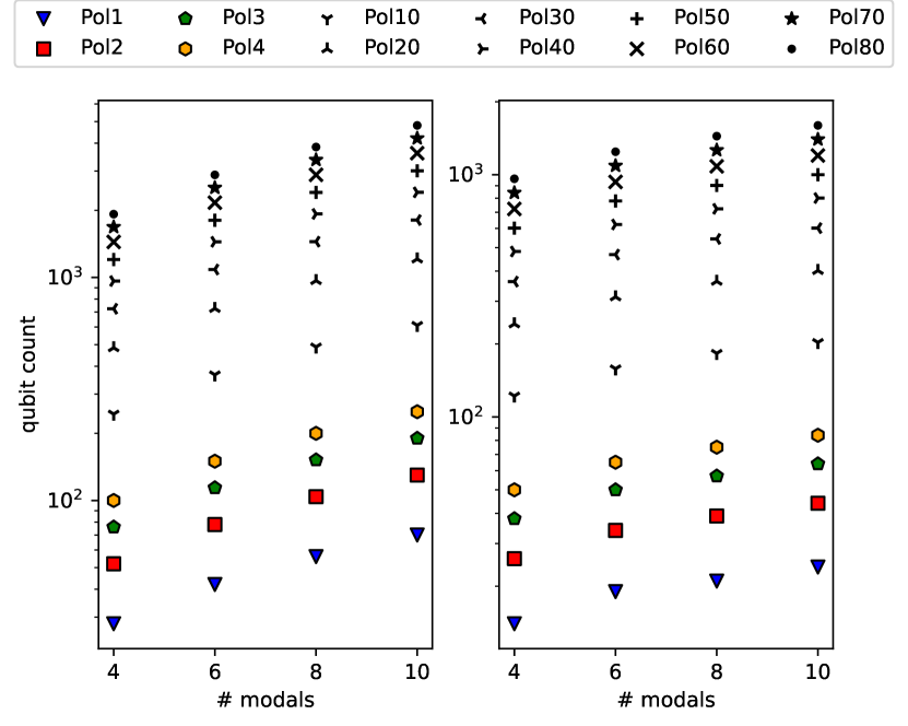
Figure 2: Qubit count in the logarithmic scale using the unary mapping (left) and binary mapping (right) for polyynes with $k$ number of triple bonds labelled as Pol$k$ for varying number of modals per vibrational mode.

4.3 Hamiltonian size

For the rest of this section, we will set the truncation order of our vibrational Hamiltonian (1) to $D=3$. The asymptotic bound (2) on the number of terms in the second-quantized Hamiltonian counts all summands in (1), including those that evaluate to zero. While only a fraction of the total number, the number of non-zero coefficients in (1) can quickly explode even for small molecules with reasonable number of modes ($L=7,13,19,\cdots$ in our case) and a limited number of modal functions ($d=4,6,8,10$). Table 3 lists the number of non-zero terms $N_{H,\neq 0}$ in the second-quantized Hamiltonian in the VSCF basis, as well the number of terms greater than $10^{-8}$ cm^-1, which will be our cutoff threshold in the qubit Hamiltonian.

Table 3: Number of terms in the second-quantized Hamiltonian for the polyyne molecules of consideration. $N_{H}$ is the number of all summands in (1); $N_{H,\neq 0}$ denotes the number of non-zero terms; and $N_{H,\geq 10^{-8}}$ denotes the number of terms that exceed $10^{-8}$ by absolute value. Note that the numbers here are for the unary encoding.

Molecule	Modals ($d$)	$N_{H}$	$N_{H,\neq 0}$	$N_{H,\geq 10^{-8}}$
acetylene	4	148848	37567	15656
acetylene	6	1660428	540684	163386
diacetylene	4	1191632	327744	117504
diacetylene	6	13445172	4860468	1277408
triacetylene	4	4013104	1255312	392952
triacetylene	6	45431964	17989164	4290852
tetraacetylene	4	9498000	3552748	916982

4.4 Trotterization cost

To keep the number of terms in the qubit Hamiltonian manageable, we favor the unary encoding (3) versus the binary one and further discard from the qubit Hamiltonian any terms with absolute value less than $10^{-8}$. This results in qubit Hamiltonian operators with number of Pauli strings roughly equal to the values of $N_{H,\geq 10^{-8}}$ reported in Table 3. While these numbers are significantly less than the total number of terms $N_{H}$, they still grow as expected, namely as (a fraction of) $L^{3}d^{6}$ (since we have fixed $D=3$). Thus, the techniques of Section 3.3 are necessary to accurately estimate the trotterization cost for these operators. Figure 3 reports the total number of Trotter steps needed to guarantee an accuracy $\epsilon_{\nu}=1cm^{-1}$, in the energies obtained with the workflow described in Section 2, for the second order ($p=2$) trotterization formula. The values in red correspond to bounds obtained with (20), while values in green are obtained with the techniques described in Section 3.3.

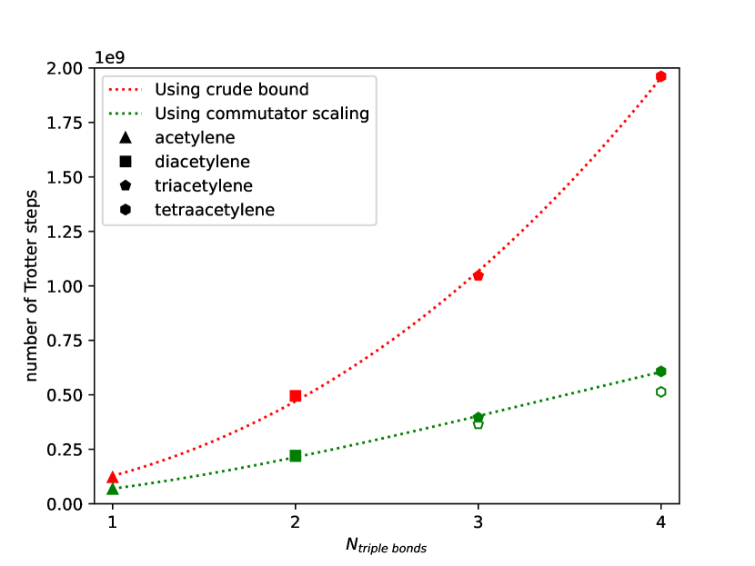
Figure 3: Estimates for the total number of Trotter steps required to achieve accuracy of $\epsilon_{\nu}=1cm^{-1}$ for the first few polyyne molecules of interest. Crude bound estimates are plotted in red and bounds using commutator scaling - in green. The solid green symbols represent an upper bound, while lower bounds are plotted with green symbol outlines. The dashed lines plot a fit to a polynomial of the type $AL^{3}+BL^{2}=A(6N_{triple\ bonds}+1)^{3}+B(6N_{triple\ bonds}+1)^{2}$, as expected from our asymptotic results. It should be noted that the best fit for the values obtained with the commutator scaling has a negative leading coefficient, suggesting that, when commutations are accounted for, the Trotter number grows only quadratically.

As expected there are significant savings in estimating the Trotter number more accurately. What is more important is that the growth of the green curve in Figure 3 seems to be of lower-order, suggesting that the savings are more than just a constant factor. Indeed, fitting a polynomial of the type $AL^{3}+BL^{2}$, which is the expected growth in (2), results in a negative leading coefficient for the values in green, obtained using the commutator-scaling approach. This suggests that these bounds grow only quadratically and the savings when compared to the crude bounds in red (which do grow cubically) will be even more noticeable for larger molecules.

4.5 Circuit parallelization

The concrete size of the Hamiltonian and the total number of Trotter steps in the QPE implementation, discussed in the subsections above, allow us to directly compute the number of gates $N_{g}$ for the Hamiltonian simulation part of the QPE circuit

$$N_{g}=\frac{gates}{per\ term}\times\frac{terms}{per\ Trotter\ step}\times{total\ number\ of\ Trotter\ steps\ required}.$$ (26)

An accurate estimate for the cost of Hamiltonian evolution in QPE, along with the number of extra ancilla qubits chosen for the accuracy of the algorithm, allows one to fully describe the complexity for the full QPE circuit in Figure 1.

The number of gates is not the sole metric for complexity. Another factor to consider in estimating the resources required for simulating each Trotter step is the depth of the circuit. Using a greedy algorithm as discussed below, we can estimate a ratio of the total number of Paulis to be simulated in each Trotter step to the number of Paulis that need to be simulated sequentially due to having overlapping support on the qubits. This ratio is a reflection of the effective reduction in circuit depth that can be obtained due to the different localities observed in the Pauli strings of the Hamiltonian.

To estimate such ratio, a Pauli string from the pool of Pauli strings to be used in the Trotter expansion is drawn at random and the set of qubits over which it acts non-trivially is compared to that of another randomly drawn Pauli string. If two sets of qubits are disjoint, then these Pauli strings can be executed simultaneously in a quantum circuit leading to no increase in depth. If the qubit sets are overlapping then the count of layers to be executed sequentially is increased by one. This procedure is continued until the Pauli pool is exhausted. A specific value for the speedup is then obtained by taking the ratio of total number of Paulis to the number of Pauli layers that need to be executed sequentially. The average expected speedup from such greedy algorithm can be computed by repeating the procedure multiple times and averaging the results.

Below we will compare these numbers for the electronic and vibrational structure problems on the acetylene molecule. Since the maximum locality of the Pauli strings in vibrational structure Hamiltonian is governed by the degree of truncation, it is independent of the number of modals in the problem. This leads to a favourable estimate of roughly 1.5 Pauli strings per unit of circuit depth for the vibrational structure Hamiltonian of the acetylene molecule truncated at the 3rd order with different number of modals. This ratio increases as the number of modals increases as expected. In comparison, the maximum locality of the Pauli strings in the electronic structure problem for most commonly used fermion-to-qubit mappings is equal to the number of qubits. On average this leads to fewer Pauli strings that can be implemented simultaneously in a quantum circuit. For the acetylene electronic structure Hamiltonian in different basis sets we find that roughly 1.1 Pauli strings can be executed at the expense of the resources required for simulation of 1 Pauli string. The exact numbers obtained from the implementation of the greedy algorithm discussed above are presented in Table 4.

Table 4: Ratio of total number of Paulis to number of Paulis that need to be simulated sequentially averaged over 100 runs, each with a different random order of selecting Paulis for the electronic and vibrational Hamiltonian of acetylene molecule.

Electronic problem	Ratio	Vibrational problem	Ratio
sto-3g	1.14539	4 modals	1.34023
6-31g	1.15238	6 modals	1.46114
cc-pvdz	1.16602	8 modals	1.60766

5 Summary and conclusion

We have provided an accurate asymptotic analysis of quantum resources required for simulating molecular vibrational structure problems on quantum computers. We have focused on an explicit Hamiltonian model, the L-mode representation of the Hamiltonian. The estimates for the quantum resources required for this Hamiltonian representation have been given in Table 2. We have used the commutator-scaling approach [10] and devised an efficient scheme to estimate the nested commutators. This has led to a tight(er) upper bound on the Trotter number requisite for simulating a particular Hamiltonian, for a given accuracy. Employing this technique, we have provided a detailed quantitative study of the quantum computational cost for concrete examples, namely, polyyne molecules.

Overall results suggest that the combined quantum resources required for achieving quantum advantage for vibrational structure problems might be lower than those for the electronic structure problems, which is in agreement with [39]. Since Pauli strings for the vibrational qubit Hamiltonian are more localized, they are expected to be easier and faster to simulate than those in the electronic qubit Hamiltonian. In addition, our estimate of the number of Pauli strings that can be simultaneously executed in a quantum circuit when implementing a single Trotter step is larger for the vibrational structure problem as compared to the electronic one. This may give the molecular vibrational simulations an edge over the electronic simulations due to higher locality of Pauli strings.

Nevertheless, further tailored studies are needed to truly compare the quantum computational cost of vibrational and electronic structure problems. Just as basis functions are employed in electronic structure, modals are utilized in the context of the vibrational structure simulations for the same purpose, see (1). Often, fewer modals are needed than basis functions. Nevertheless, as shown in Table 2, their number greatly affects the required quantum resources. Furthermore, the number of modals required for a vibrational structure problem increases with temperature. While the number of relevant terms in the vibrational qubit Hamiltonian may be smaller from an asymptotic perspective, the situation is not as clean-cut for molecules that we can reasonably expect to be able to study on quantum devices in the near term, see Table 5 in Appendix B. Determining the chemical components and properties where either vibrational or electronic structure simulation can lead to quantum advantage requires a thorough case-by-case study.

In light of the discussion presented in this paper, in our opinion, it is not yet clear what is the best frame for comparing molecular electronic and vibrational structure problems, in order to determine which one would offer quantum advantage first. Rather than comparing the quantum resource requirements for problems resulting in similarly sized Hilbert spaces, one can, for example, compare it for selected sets of small challenging problems from each domain (and their respective chemical accuracy). Considering that the electronic structure problems on quantum computers are somewhat well-understood, however, for such comparison to be meaningful we will need a better understanding of possible optimizations that could improve the qubit numbers and the circuit depth for the vibrational structure simulations as well.

Appendix A: Vibrational self-consistent field method

Vibrational self-consistent field (VSCF) is a time-independent form of self-consistent field method. The method is implemented in the MidasCpp (Molecular Interactions, Dynamics and Simulation in C++/Chemistry Program Package) [11] and provides the reference state and optimal single-mode basis functions (modals). For a system with $L$ modes, the VSCF ansatz for the wave function is given by

$$\left|\Phi_{\rm VSCF}\right\rangle=e^{\kappa}\left|\Phi_{\mathbf{R}}\right\rangle==\exp\left(\sum_{l=1}^{L}\sum_{k_{l}\,h_{l}}\kappa_{k_{l}h_{l}}\mathcal{E}_{k_{l}h_{l}}\right)\left|\Phi_{\mathbf{R}}\right\rangle\,,$$ (27)

with the reference state being

$$\left|\Phi_{\mathbf{R}}\right\rangle=\prod_{l}^{L}a_{R_{l}}^{\dagger}\,\left|\rm{vac}\right\rangle\,.$$ (28)

The vector $\mathbf{R}$ specifies the mode that modal is occupied in the reference state and ${\mathcal{E}}_{k_{l}h_{l}}=a_{k_{l}}^{\dagger}a_{h_{l}}$, with $a_{k_{l}}^{\dagger}$ and $a_{h_{l}}$ being the bosonic creation and annihilation operators, respectfully, and $a_{h_{l}}\left|\rm vac\right\rangle=0$. The operator $\kappa$ is anti-hermitian and $\exp(\kappa)$ is unitary. The exponential prefactor generates rotations among the modals. The optimal VSCF modals are obtained by implementing the variational principle on the modal rotation parameters ($\kappa_{k_{l}h_{l}}$) of the VSCF energy $E_{\rm VSCF}=\left\langle\Phi_{\mathbf{R}}\right|\exp(-\kappa)H\exp(\kappa)\left|\Phi_{\mathbf{R}}\right\rangle$:

$$\frac{\partial}{\partial\kappa_{k_{l}h_{l}}}\left\langle\Phi_{\mathbf{R}}\right|\exp(-\kappa)H\exp(\kappa)\left|\Phi_{\mathbf{R}}\right\rangle=0.$$ (29)

By inserting the VSCF ansatz in this equation, one can obtain

$$\left\langle\Phi_{\mathbf{R}}\right|\,[H,{\mathcal{E}}_{k_{l}h_{l}}]\,\left|\Phi_{\mathbf{R}}\right\rangle=0$$ (30)

as a criterion for having an optimal $\left|\Phi_{\mathbf{R}}\right\rangle$ for $\kappa=0$. Then one can assign an effective mean-field operator for mode $l$,

$$F^{l,\mathbf{R}}_{k_{l}h_{l}}=\left\langle\Phi_{\mathbf{R}}\right|\,[[a_{k_{l}},H],a_{h_{l}}^{\dagger}]\,\left|\Phi_{\mathbf{R}}\right\rangle.$$ (31)

Employing the second quantization commutator relations, the $F^{l,\mathbf{R}}$ matrix elements would be directly related to the VSCF gradient terms where a zero gradient can be obtained by diagonalizing the $F^{l,\mathbf{R}}$ matrix. Then solving the VSCF equations for a given Hamiltonian means constructing the $F^{l,\mathbf{R}}$ matrix, diagonalizing it, updating the Hamiltonian parameters, calculating the VSCF energy and checking the convergence; see [16, 13] for more details.

The other simpler but less accurate approach here is harmonic approximation, where states $\left|\Phi\right\rangle$ are the eigenfunctions of a harmonic oscillator for each mode. Then the one-body and two-body integrals in Eq. (1) can be expressed as a Taylor expansion and are easy to calculate. These integrals are implemented in Qiskit [2].

Appendix B:

Table 5: Number of terms for different type of simulations based on the required number of qubits. The cut-off for the electronic structure simulations is 10^-8 hartree while it is 10^-5 cm^-1 for the vibrational structure ones.

Qubits	Molecule	Simulation Type	Basis Functions/number of Modals	Pauli Terms
10	LiH	electronic structure	sto-3g	276
12	H2O	electronic structure	sto-3g	551
20	C2H2 or P1	electronic structure	sto-3g	2951
20	LiH	electronic structure	6-31g	5851
24	H2O	electronic structure	6-31g	8921
28	C2H2 or P1	vibrational structure	4 modals	15657
32	N2	electronic structure	6-31g	21521
36	LiH	electronic structure	cc-pvdz	63519
40	C2H2 or P1	electronic structure	6-31g	53289
42	C2H2 or P1	vibrational structure	6 modals	155279
46	H2O	electronic structure	cc-pvdz	107382
52	N2	electronic structure	cc-pvdz	145327
52	P2	vibrational structure	4 modals	114948
56	C2H2 or P1	vibrational structure	8 modals	693419
72	C2H2 or P1	electronic structure	cc-pvdz	542433
76	P3	vibrational structure	4 modals	376974
78	P2	vibrational structure	6 modals	1044058
104	P2	vibrational structure	8 modals	4386132
114	P3	vibrational structure	6 modals	3277705

References

- [1] NIST Chemistry WebBook, NIST Standard Reference Database Number 69. doi: https://doi.org/10.18434/T4D303. URL https://webbook.nist.gov.
- Abraham et al. [2019] Héctor Abraham et al. Qiskit: An open-source framework for quantum computing, 2019.
- Aspuru-Guzik et al. [2005] Alán Aspuru-Guzik, Anthony D. Dutoi, Peter J. Love, and Martin Head-Gordon. Simulated quantum computation of molecular energies. Science, 309(5741):1704–1707, 2005.
- Babbush et al. [2018] Ryan Babbush, Craig Gidney, Dominic W Berry, Nathan Wiebe, Jarrod McClean, Alexandru Paler, Austin Fowler, and Hartmut Neven. Encoding electronic spectra in quantum circuits with linear t complexity. Physical Review X, 8(4):041015, 2018.
- Bowman et al. [2003] Joel M. Bowman, Stuart Carter, and Xinchuan Huang. Multimode: A code to calculate rovibrational energies of polyatomic molecules. International Reviews in Physical Chemistry, 22(3):533–549, 2003.
- Bravyi and Kitaev [2002] Sergey B. Bravyi and Alexei Yu. Kitaev. Fermionic quantum computation. Annals of Physics, 298:210–226, 2002.
- Cao et al. [2019] Yudong Cao, Jonathan Romero, Jonathan P. Olson, Matthias Degroote, Peter D. Johnson, Mária Kieferová, Ian D. Kivlichan, Tim Menke, Borja Peropadre, Nicolas P. D. Sawaya, Sukin Sim, Libor Veis, and Alán Aspuru-Guzik. Quantum chemistry in the age of quantum computing. Chemical Reviews, 119(19):10856–10915, 2019.
- Cerezo et al. [2021] M. Cerezo, Andrew Arrasmith, Ryan Babbush, Simon C. Benjamin, Suguru Endo, Keisuke Fujii, Jarrod R. McClean, Kosuke Mitarai, Xiao Yuan, Lukasz Cincio, and Patrick J. Coles. Variational quantum algorithms. Nature Reviews Physics, 3(9):625–644, 2021.
- Chalifoux and Tykwinski [2010] Wesley A Chalifoux and Rik R Tykwinski. Synthesis of polyynes to model the sp-carbon allotrope carbyne. Nature chemistry, 2(11):967, 2010.
- Childs et al. [2021] Andrew M Childs, Yuan Su, Minh C Tran, Nathan Wiebe, and Shuchen Zhu. Theory of trotter error with commutator scaling. Physical Review X, 11(1):011020, 2021.
- Christiansen et al. [version 2022.10.0] Ove Christiansen, Denis G. Artiukhin, Frederik Bader, Ian H. Godtliebsen, Eduard M. Gras, Werner Győrffy, Mikkel B. Hansen, Mads B. Hansen, Mads G. Højlund, Nicolai M. Høyer, Rasmus B. Jensen, Andreas B. Jensen, Emil L. Klinting, Jacob Kongsted, Carolin König, Diana Madsen, Niels K. Madsen, Kasper Monrad, Gunar Schmitz, Peter Seidler, Kristian Sneskov, Manuel Sparta, Bo Thomsen, Daniele Toffoli, and Alberto Zoccante. Midascpp: Molecular interactions dynamics and simulation, version 2022.10.0. URL https://midascpp.gitlab.io/pages/manual.html.
- Cramer [2004] Cristopher J. Cramer. Essentials of Computational Chemistry: Theories and Models. John Wiley & Sons, Ltd, 2004. ISBN 978-0-470-09182-1.
- Császár [2012] Attila G. Császár. Anharmonic molecular force fields. WIREs Comput Mol Sci, 2:273–289, 2012.
- Dalzell et al. [2023] Alexander M. Dalzell, Sam McArdle, Mario Berta, Przemyslaw Bienias, Chi-Fang Chen, András Gilyén, Connor T. Hann, Michael J. Kastoryano, Emil T. Khabiboulline, Aleksander Kubica, Grant Salton, Samson Wang, and Fernando G. S. L. Brandão. Quantum algorithms: A survey of applications and end-to-end complexities. arXiv:2310.03011, 2023.
- Dresselhaus et al. [2000] Mildred S Dresselhaus, Gene Dresselhaus, PC Eklund, and AM Rao. Carbon nanotubes. In The physics of fullerene-based and fullerene-related materials, pages 331–379. Springer, 2000.
- Hansen et al. [2010] Mikkel B Hansen, Manuel Sparta, Peter Seidler, Daniele Toffoli, and Ove Christiansen. New formulation and implementation of vibrational self-consistent field theory. Journal of chemical theory and computation, 6(1):235–248, 2010.
- Helgaker et al. [2000] Trygve Helgaker, Poul Jørgensen, and Jeppe Olsen. Molecular Electronic‐Structure Theory. John Wiley & Sons, Ltd, 2000. ISBN 9781119019572.
- Jahangiri et al. [2020] Soran Jahangiri, Juan M. Arrazola, Nicolás Quesada, and Alain Delgado. Quantum algorithm for simulating molecular vibrational excitations. Phys. Chem. Chem. Phys., 22:25528–25537, 2020.
- Jensen [2017] Frank Jensen. Introduction to Computational Chemistry. John Wiley & Sons, Ltd, 2017. ISBN 978-1-118-82599-0.
- Kandala et al. [2017] Abhinav Kandala, Antonio Mezzacapo, Kristan Temme, Maika Takita, Markus Brink, Jerry M. Chow, and Jay M. Gambetta. Hardware-efficient variational quantum eigensolver for small molecules and quantum magnets. Nature, 549(7671):242–246, 2017.
- Kinloch et al. [2018] Ian A Kinloch, Jonghwan Suhr, Jun Lou, Robert J Young, and Pulickel M Ajayan. Composites with carbon nanotubes and graphene: An outlook. Science, 362(6414):547–553, 2018.
- Laidler [1987] Keith James Laidler. Chemical Kinetics. Prentice Hall, 3rd Revised ed edition, 1987. ISBN 978-0060438623.
- Lanyon et al. [2010] Benjamin P. Lanyon, James D. Whitfield, Geoff G. Gillett, Michael E. Goggin, Marcelo P. Almeida, Ivan Kassal, Jacob D. Biamonte, Masoud Mohseni, Ben J. Powell, Marco Barbieri, Alán Aspuru-Guzik, and Andrew G. White. Towards quantum chemistry on a quantum computer. Nature Chemistry, 2(2):106–111, 2010.
- Leach [2001] Andrew R. Leach. Molecular Modelling: Principles and Applications. Pearson, 2001. ISBN 978-0582382107.
- Lee et al. [1995] Timothy J. Lee, Jan M. L. Martin, and Peter R. Taylor. An accurate ab initio quartic force field and vibrational frequencies for ch4 and isotopomers. J. Chem. Phys., 102:254, 1995.
- Li et al. [2001] Genyuan Li, Carey Rosenthal, and Herschel Rabitz. High dimensional model representations. The Journal of Physical Chemistry A, 105(33):7765–7777, 2001.
- Liu et al. [2022] Hongbin Liu, Guang Hao Low, Damian S. Steiger, Thomas Häner, Markus Reiher, and Matthias Troyer. Prospects of quantum computing for molecular sciences. Materials Theory, 6(1):11, 2022.
- Magann et al. [2021] Alicia B. Magann, Matthew D. Grace, Herschel A. Rabitz, and Mohan Sarovar. Digital quantum simulation of molecular dynamics and control. Phys. Rev. Research, 3:023165, 2021.
- Majland et al. [2022] Marco Majland, Rasmus B. Jensen, Mads G. Højlund, Nikolaj T. Zinner, and Ove Christiansen. Runtime optimization for vibrational structure on quantum computers: coordinates and measurement schemes. arXiv:2211.11615, 2022.
- Marzari et al. [2021] Nicola Marzari, Andrea Ferretti, and Chris Wolverton. Electronic-structure methods for materials design. Nature Materials, 20(6):736–749, 2021.
- Milani et al. [2011] Alberto Milani, Andrea Lucotti, Valeria Russo, M Tommasini, Francesco Cataldo, Andrea Li Bassi, and Carlo Spartaco Casari. Charge transfer and vibrational structure of sp-hybridized carbon atomic wires probed by surface enhanced raman spectroscopy. The Journal of Physical Chemistry C, 115(26):12836–12843, 2011.
- Nielsen and Chuang [2011] Michael A. Nielsen and Isaac L. Chuang. Quantum Computation and Quantum Information: 10th Anniversary Edition. Cambridge University Press, USA, 10th edition, 2011. ISBN 1107002176.
- Ollitrault et al. [2020] Pauline J. Ollitrault, Alberto Baiardi, Markus Reiher, and Ivano Tavernelli. Hardware efficient quantum algorithms for vibrational structure calculations. Chem. Sci., 11:6842–6855, 2020.
- Peruzzo et al. [2014] Alberto Peruzzo, Jarrod McClean, Peter Shadbolt, Man-Hong Yung, Xiao-Qi Zhou, Peter J. Love, Alán Aspuru-Guzik, and Jeremy L. O’Brien. A variational eigenvalue solver on a photonic quantum processor. Nature Communications, 5(1):4213, 2014.
- Reiher et al. [2017] Markus Reiher, Nathan Wiebe, Krysta M. Svore, Dave Wecker, and Matthias Troyer. Elucidating reaction mechanisms on quantum computers. Proceedings of the national academy of sciences, 114(29):7555–7560, 2017.
- Richerme et al. [2023] Philip Richerme, Melissa C. Revelle, Debadrita Saha, Miguel A. Lopez-Ruiz, Anurag Dwivedi, Sam A. Norrell, Christopher G. Yale, Daniel Lobser, Ashlyn D. Burch, Susan M. Clark, Jeremy M. Smith, Amr Sabry, and Srinivasan S. Iyengar. Quantum computation of hydrogen bond dynamics and vibrational spectra. arXiv:2204.08571, 2023.
- Sawaya and Huh [2019] Nicolas P. D. Sawaya and Joonsuk Huh. Quantum algorithm for calculating molecular vibronic spectra. J. Phys. Chem. Lett., 10(13):3586–3591, 2019.
- Sawaya et al. [2020] Nicolas P. D. Sawaya, Tim Menke, Thi Ha Kyaw, Sonika Johri, Alán Aspuru-Guzik, and Gian Giacomo Guerreschi. Resource-efficient digital quantum simulation of d-level systems for photonic, vibrational, and spin-s hamiltonians. npj Quantum Information, 6(49), 2020.
- Sawaya et al. [2021] Nicolas P. D. Sawaya, Francesco Paesani, and Daniel P. Tabor. Near- and long-term quantum algorithmic approaches for vibrational spectroscopy. Phys. Rev. A, 104:062419, 2021.
- Sparrow et al. [2018] C. Sparrow, E. Martín-López, N. Maraviglia, A. Neville, C. Harrold, J. Carolan, Y. N. Joglekar, T. Hashimoto, N. Matsuda, J. L. O’Brien, D. P. Tew, and A. Laing. Simulating the vibrational quantum dynamics of molecules using photonics. Nature, 557(7707):660–667, 2018.
- Sumathi and Green Jr. [2002] R. Sumathi and William H. Green Jr. A priori rate constants for kinetic modeling. Theoretical Chemistry Accounts, 108:187–213, 2002.