Loss Balancing for Fair Supervised Learning

Abstract

Supervised learning models have been used in various domains such as lending, college admission, face recognition, natural language processing, etc. However, they may inherit pre-existing biases from training data and exhibit discrimination against protected social groups. Various fairness notions have been proposed to address unfairness issues. In this work, we focus on Equalized Loss (EL), a fairness notion that requires the expected loss to be (approximately) equalized across different groups. Imposing EL on the learning process leads to a non-convex optimization problem even if the loss function is convex, and the existing fair learning algorithms cannot properly be adopted to find the fair predictor under the EL constraint. This paper introduces an algorithm that can leverage off-the-shelf convex programming tools (e.g., CVXPY (Diamond and Boyd, 2016; Agrawal et al., 2018)) to efficiently find the global optimum of this non-convex optimization. In particular, we propose the ELminimizer algorithm, which finds the optimal fair predictor under EL by reducing the non-convex optimization to a sequence of convex optimization problems. We theoretically prove that our algorithm finds the global optimal solution under certain conditions. Then, we support our theoretical results through several empirical studies.

1 Introduction

As machine learning (ML) algorithms are increasingly being used in applications such as education, lending, recruitment, healthcare, criminal justice, etc., there is a growing concern that the algorithms may exhibit discrimination against protected population groups. For example, speech recognition products such as Google Home and Amazon Alexa were shown to have accent bias (Harwell, 2018). The COMPAS recidivism prediction tool, used by courts in the US in parole decisions, has been shown to have a substantially higher false positive rate for African Americans compared to the general population (Dressel and Farid, 2018). Amazon had been using automated software since 2014 to assess applicants’ resumes, which were found to be biased against women (Dastin, 2018). As a result, there have been several works focusing on interpreting machine learning models to understand how features and sensitive attributes contribute to the output of the model (Ribeiro et al., 2016; Lundberg and Lee, 2017; Abroshan et al., 2023).

Various fairness notions have been proposed in the literature to measure and remedy the biases in ML systems; they can be roughly classified into two categories: 1) individual fairness focuses on equity at the individual level and it requires similar individuals to be treated similarly (Dwork et al., 2012; Biega et al., 2018; Jung et al., 2019; Gupta and Kamble, 2019); 2) group fairness requires certain statistical measures to be (approximately) equalized across different groups distinguished by some sensitive attributes (Hardt et al., 2016; Conitzer et al., 2019; Khalili et al., 2020; Zhang et al., 2020; Khalili et al., 2021; Diana et al., 2021; Williamson and Menon, 2019; Zhang et al., 2022).

Several approaches have been developed to satisfy a given definition of fairness; they fall under three categories: 1) pre-processing, by modifying the original dataset such as removing certain features and reweighing, (e.g., (Kamiran and Calders, 2012; Celis et al., 2020; Abroshan et al., )); 2) in-processing, by modifying the algorithms such as imposing fairness constraints or changing objective functions during the training process, (e.g., (Zhang et al., 2018; Agarwal et al., 2018, 2019; Reimers et al., 2021; Calmon et al., 2017)); 3) post-processing, by adjusting the output of the algorithms based on sensitive attributes, (e.g., (Hardt et al., 2016)).

In this paper, we focus on group fairness, and we aim to mitigate unfairness issues in supervised learning using an in-processing approach. This problem can be cast as a constrained optimization problem by minimizing a loss function subject to a group fairness constraint. We are particularly interested in the Equalized Loss (EL) fairness notion proposed by Zhang et al. (2019), which requires the expected loss (e.g., Mean Squared Error (MSE), Binary Cross Entropy (BCE) Loss) to be equalized across different groups.

The problem of finding fair predictors by solving constrained optimizations has been largely studied. Komiyama et al. (2018) propose the coefficient of determination constraint for learning a fair regressor and develop an algorithm for minimizing the mean squared error (MSE) under their proposed fairness notion. Agarwal et al. (2019) propose an approach to finding a fair regression model under bounded group loss and statistical parity fairness constraints. Agarwal et al. (2018) study classification problems and aim to find fair classifiers under various fairness notions including statistical parity and equal opportunity. In particular, they consider zero-one loss as the objective function and train a randomized fair classifier over a finite hypothesis space. They show that this problem can be reduced to a problem of finding the saddle point of a linear Lagrangian function. Zhang et al. (2018) propose an adversarial debiasing technique to find fair classifiers under equalized odd, equal opportunity, and statistical parity. Unlike the previous works, we focus on the Equalized Loss fairness notion which has not been well studied. Finding an EL fair predictor requires solving a non-convex optimization. Unfortunately, there is no algorithm in fair ML literature with a theoretical performance guarantee that can be properly applied to EL fairness (see Section 2 for detailed discussion).

Our main contribution can be summarized as follows,

• We develop an algorithm with a theoretical performance guarantee for EL fairness. In particular, we propose the $(\texttt{ELminimizer})$ algorithm to solve a non-convex constrained optimization problem that finds the optimal fair predictor under EL constraint. We show that such a non-convex optimization problem can be reduced to a sequence of convex constrained optimizations. The proposed algorithm finds the global optimal solution and is applicable to both regression and classification problems. Importantly, it can be easily implemented using off-the-shelf convex programming tools.

• In addition to ELminimizer which finds the global optimal solution, we develop a simple algorithm for finding a sub-optimal predictor satisfying EL fairness. We prove there is a sub-optimal solution satisfying EL fairness that is a linear combination of the optimal solutions to two unconstrained optimizations, and it can be found without solving any constrained optimizations.

• We conduct sample complexity analysis and provide a generalization performance guarantee. In particular, we show the sample complexity analysis found in (Donini et al., 2018) is applicable to learning problems under EL.

• We also examine (in the appendix) the relation between Equalized Loss (EL) and Bounded Group Loss (BGL), another fairness notion proposed by (Agarwal et al., 2019). We show that under certain conditions, these two notions are closely related, and they do not contradict each other.

2 Problem Formulation

Consider a supervised learning problem where the training dataset consists of triples $(\boldsymbol{X},A,Y)$ from two social groups. Random variable $\boldsymbol{X}\in\mathcal{X}$ is the feature vector (in the form of a column vector), $A\in\{0,1\}$ is the sensitive attribute (e.g., race, gender) indicating the group membership, and $Y\in\mathcal{Y}\subseteq\mathbb{R}$ is the label/output.We denote realizations of random variables by small letters (e.g., $(\boldsymbol{x},a,y)$ is a realization of $(\boldsymbol{X},A,Y)$). Feature vector $\boldsymbol{X}$ may or may not include sensitive attribute $A$. Set $\mathcal{Y}$ can be either $\{0,1\}$ or $\mathbb{R}$: if $\mathcal{Y}=\{0,1\}$ (resp. $\mathcal{Y}=\mathbb{R}$), then the problem of interest is a binary classification (resp. regression) problem.

Let $\mathcal{F}$ be a set of predictors $f_{\boldsymbol{w}}:\mathcal{X}\to\mathbb{R}$ parameterized by weight vector $\boldsymbol{w}$ with dimension $d_{\boldsymbol{w}}$. If the problem is binary classification, then $f_{\boldsymbol{w}}(\boldsymbol{x})$ is an estimate of $\Pr(Y=1|\boldsymbol{X}=\boldsymbol{x})$. Consider loss function $l:\mathcal{Y}\times\mathbb{R}\to\mathbb{R}$ where $l(Y,f_{\boldsymbol{w}}(\boldsymbol{X}))$ measures the error of $f_{\boldsymbol{w}}$ in predicting $\boldsymbol{X}$. We denote the expected loss with respect to the joint probability distribution of $(\boldsymbol{X},Y)$ by $L(\boldsymbol{w}):=\mathbb{E}\{l(Y,f_{\boldsymbol{w}}(\boldsymbol{X}))\}$. Similarly, $L_{a}(\boldsymbol{w}):=\mathbb{E}\{l(Y,f_{\boldsymbol{w}}(\boldsymbol{X}))|A=a\}$ denotes the expected loss of the group with sensitive attribute $A=a$. In this work, we assume that $l(y,f_{\boldsymbol{w}}(\boldsymbol{x}))$ is differentiable and strictly convex in ${\boldsymbol{w}}$ (e.g., binary cross entropy loss).

Without fairness consideration, a predictor that simply minimizes the total expected loss, i.e., $\operatorname*{arg\,min}_{\boldsymbol{w}}L(\boldsymbol{w})$, may be biased against certain groups. To mitigate the risks of unfairness, we consider Equalized Loss (EL) fairness notion, as formally defined below.

Definition 2.1 ($\gamma$-EL (Zhang et al., 2019)).

We say $f_{\boldsymbol{w}}$ satisfies the equalized loss (EL) fairness notion if $L_{0}({\boldsymbol{w}})=L_{1}({\boldsymbol{w}})$. Moreover, we say $f_{\boldsymbol{w}}$ satisfies $\gamma-$EL for some $\gamma>0$ if $-\gamma\leq L_{0}({\boldsymbol{w}})-L_{1}({\boldsymbol{w}})\leq\gamma$.

Note that if $l(Y,f_{\boldsymbol{w}}(\boldsymbol{X}))$ is a (strictly) convex function in $\boldsymbol{w}$, both $L_{0}(\boldsymbol{w})$ and $L_{1}(\boldsymbol{w})$ are also (strictly) convex in ${\boldsymbol{w}}$. However, $L_{0}(\boldsymbol{w})-L_{1}(\boldsymbol{w})$ is not necessary convex. As a result, the following optimization problem for finding a fair predictor under $\gamma$-EL is not a convex programming,

$$\min_{\boldsymbol{w}}~{}~{}L(\boldsymbol{w})~{}\text{ s.t.}~{}~{}-\gamma\leq L_{0}(\boldsymbol{w})-L_{1}(\boldsymbol{w})\leq\gamma.$$ (1)

We say a group is disadvantaged group if it experiences higher loss than the other group. Before discussing how to find the global optimal solution of the above non-convex optimization problem and train a $\gamma$-EL fair predictor, we first discuss why $\gamma$-EL is an important fairness notion and why the majority of fair learning algorithms in the literature cannot be used for finding $\gamma$-EL fair predictors.

2.1 Existing Fairness Notions & Algorithms

Next, we (mathematically) introduce some of the most commonly used fairness notions and compare them with $\gamma$-EL. We will also discuss why the majority of proposed fair learning algorithms are not properly applicable to EL fairness.

Overall Misclassification Rate (OMR): It was considered by (Zafar et al., 2017, 2019) for classification problems. Let $\hat{Y}=I(f_{\boldsymbol{w}}(\boldsymbol{X})>0.5)$, where $I(.)\in\{0,1\}$ is an indicator function, and $\hat{Y}=1$ if $f_{\boldsymbol{w}}(\boldsymbol{X})>0.5$. OMR requires $\Pr(\hat{Y}\neq Y|A=0)=\Pr(\hat{Y}\neq Y|A=1),$ which is not a convex constraint. As a result, Zafar et al. (2017; 2019) propose a method to relax this constraint using decision boundary covariances. We emphasize that OMR is different from EL fairness, that OMR only equalizes the accuracy of binary predictions across different groups while EL is capable of considering the fairness in estimating probability $\Pr(Y=1|\boldsymbol{X}=\boldsymbol{x})$, e.g., by using binary cross entropy loss function. Note that in many applications such as conversion prediction, click prediction, medical diagnosis, etc., it is critical to find $\Pr(Y=1|\boldsymbol{X}=\boldsymbol{x})$ accurately for different groups besides the final predictions $\hat{Y}$. Moreover, unlike EL, OMR is not applicable to regression problems. Therefore, the relaxation method proposed by (Zafar et al., 2017, 2019) cannot be applied to the EL fairness constraint.

Statistical Parity (SP), Equal Opportunity (EO): For binary classification, Statistical Parity (SP) (Dwork et al., 2012) (resp. Equal Opportunity (EO) (Hardt et al., 2016)) requires the positive classification rates (resp. true positive rates) to be equalized across different groups. Formally,

$$\Pr(\hat{Y}=1|A=0) = \Pr(\hat{Y}=1|A=1)$$

$$\Pr(\hat{Y}=1|A=0,Y=1) = \Pr(\hat{Y}=1|A=1,Y=1)$$

Both notions can be re-written in the expectation form using an indicator function. Specifically, SP is equivalent to $\mathbb{E}\{I(f_{\boldsymbol{w}}(\boldsymbol{X})>0.5)|A=0\}=\mathbb{E}\{I(f_{\boldsymbol{w}}(\boldsymbol{X})>0.5)|A=1\}$, and EO equals to $\mathbb{E}\{I(f_{\boldsymbol{w}}(\boldsymbol{X})>0.5)|A=0,Y=1\}=\mathbb{E}\{I(f_{\boldsymbol{w}}(\boldsymbol{X})>0.5)|A=1,Y=1\}$. Since the indicator function is neither differentiable nor convex, Donini et al. (2018) use a linear relaxation of EO as a proxy. However, linear relaxation may negatively affect the fairness of the predictor (Lohaus et al., 2020). To address this issue, Lohaus et al. (2020) and Wu et al. (2019) develop convex relaxation techniques for SP and EO fairness criteria by convexifying indicator function $I(.)$. However, these convex relaxation techniques are not applicable to EL fairness notion because $l(.,.)$ in our setting is convex, not a zero-one function. FairBatch (Roh et al., 2020) is another algorithm that has been proposed to find a predictor under SP or EO. FairBatch adds a sampling bias in the mini-batch selection. However, the bias in mini-batch sampling distribution leads to a biased estimate of the gradient, and there is no guarantee FairBatch finds the global optimum solution. FairBatch can be used to find a sub-optimal fair predictor EL fairness notion. We use FairBatch as a baseline. Shen et al. (2022) propose an algorithm for EO. This algorithm adds a penalty term to the objective function, which is similar to the Penalty Method (Ben-Tal and Zibulevsky, 1997). We will use the Penalty method as a baseline as well.

Hardt et al. (2016) propose a post-processing algorithm that randomly flips the binary predictions to satisfy EO or SP. However, this method does not guarantee finding an optimal classifier (Woodworth et al., 2017). Agarwal et al. (2018) introduce a reduction approach for SP or EO. However, this method finds a randomized classifier satisfying SP or EO in expectation. In other words, to satisfy SP, the reduction approach finds distribution $Q$ over $\mathcal{F}$ such that,

$$\textstyle\sum_{f\in\mathcal{F}}Q(f)\mathbb{E}\{l(Y,f(\boldsymbol{X}))|A=0\}$$

$$\textstyle=\sum_{f\in\mathcal{F}}Q(f)\mathbb{E}\{l(Y,f(\boldsymbol{X}))|A=1\}$$

where $Q(f)$ is the probability of selecting model $f$ under distribution $Q$. Obviously, satisfying a fairness constraint in expectation may lead to unfair predictions because $Q$ can still assign a non-zero probability to unfair models.

In summary, maybe some of the approaches used for SP/EO are applicable to EL fairness notion (e.g., linear relaxation or FairBatch). However, they can only find sub-optimal solutions (see Section 6 for more details).

Statistical Parity for Regression: SP can be adjusted to be suitable for regression. As proposed by (Agarwal et al., 2019), Statistical Parity for regressor $f_{\boldsymbol{w}}(.)$ is defined as:

$$\Pr(f_{\boldsymbol{w}}(\boldsymbol{X})\leq z|A=a)=\Pr(f_{\boldsymbol{w}}(\boldsymbol{X})\leq z),\forall z,a.$$ (2)

To find a predictor that satisfies constraint (2), Agarwal et al. (2019) use the reduction approach as mentioned above. However, this approach only finds a randomized predictor satisfying SP in expectation and cannot be applied to optimization problem (1).

Bounded Group Loss (BGL): $\gamma$-BGL was introduced by (Agarwal et al., 2019) for regression problems. It requires that the loss experienced by each group be bounded by $\gamma$. That is, $L_{a}(\boldsymbol{w})\leq\gamma,\forall a\in\{0,1\}.$ Agarwal et al. (2019) use the reduction approach to find a randomized regression model under $\gamma$-BGL. In addition to the reduction method, if $L(\boldsymbol{w})$, $L_{0}(\boldsymbol{w})$, and $L_{1}(\boldsymbol{w})$ are convex in $\boldsymbol{w}$, then we can directly use convex solvers (e.g., CVXPY (Diamond and Boyd, 2016; Agrawal et al., 2018)) to find a $\gamma$-BGL fair predictor. This is because the following is a convex problem,

$$\min_{\boldsymbol{w}}L({\boldsymbol{w}}),~{}~{}~{}\text{s.t.},~{}~{}~{}L_{a}(\boldsymbol{w})\leq\gamma,~{}\forall a.$$ (3)

However, for non-convex optimization problems such as (1), the convex solvers cannot be used directly.

We want to emphasize that even though there are already many fairness notions and algorithms in the literature to find a fair predictor, none of the existing algorithms can be used to solve the non-convex optimization (1) efficiently and find a global optimal fair predictor under EL notion.

3 Optimal Model under $\gamma$-EL

In this section, we consider optimization problem (1) under EL fairness constraint. Note that this optimization problem is non-convex and finding the global optimal solution is difficult. We propose an algorithm that finds the solution to non-convex optimization (1) by solving a sequence of convex optimization problems. Before presenting the algorithm, we first introduce two assumptions, which will be used when proving the convergence of the proposed algorithm.

Algorithm 1 Function ELminimizer

Input: $\boldsymbol{w}_{G_{0}},\boldsymbol{w}_{G_{1}},\epsilon,\gamma$
Parameters: $\lambda_{start}^{(0)}=L_{0}(\boldsymbol{w}_{G_{0}}),\lambda_{end}^{(0)}=L_{0}(\boldsymbol{w}_{G_{1}}),i=0$
Define $\tilde{L}_{1}(\boldsymbol{w})=L_{1}(\boldsymbol{w})+\gamma$

1:  while $\lambda^{(i)}_{end}-\lambda^{(i)}_{start}>\epsilon$ do

2:     $\lambda^{(i)}_{mid}=(\lambda^{(i)}_{end}+\lambda^{(i)}_{start})/2$

3:     Solve the following convex optimization problem,

$$\boldsymbol{w}_{i}^{*}=\arg\min_{\boldsymbol{w}}\tilde{L}_{1}(\boldsymbol{w})~{}~{}\text{s.t.}~{}~{}L_{0}(\boldsymbol{w})\leq\lambda^{(i)}_{mid}$$ (4)

4:     $\lambda^{(i)}=\tilde{L}_{1}(\boldsymbol{w}_{i}^{*})$

5:     if $\lambda^{(i)}\geq\lambda^{(i)}_{mid}$ then

6:        $\lambda^{(i+1)}_{start}=\lambda^{(i)}_{mid}$;  $\lambda^{(i+1)}_{end}=\lambda^{(i)}_{end}$;

7:     else

8:        $\lambda^{(i+1)}_{end}=\lambda^{(i)}_{mid}$;  $\lambda^{(i+1)}_{start}=\lambda^{(i)}_{start}$;

9:        $i=i+1$;

10:     end if

11:  end while

Output: $\boldsymbol{w}_{i}^{*}$

Assumption 3.1.

Expected losses $L_{0}(\boldsymbol{w})$, $L_{1}(\boldsymbol{w})$, and $L(\boldsymbol{w})$ are strictly convex and differentiable in $\boldsymbol{w}$. Moreover, each of them has a unique minimizer.

Let $\boldsymbol{w}_{G_{a}}$ be the optimal weight vector minimizing the loss associated with group $A=a$. That is,

$$\boldsymbol{w}_{G_{a}}=\arg\min_{\boldsymbol{w}}L_{a}(\boldsymbol{w}).$$ (5)

Since problem (5) is an unconstrained, convex optimization problem, $\boldsymbol{w}_{G_{a}}$ can be found efficiently by common convex solvers. We make the following assumption about $\boldsymbol{w}_{G_{a}}$.

Assumption 3.2.

We assume the following holds,

$$L_{0}(\boldsymbol{w}_{G_{0}})\leq L_{1}(\boldsymbol{w}_{G_{0}})\text{ and }L_{1}(\boldsymbol{w}_{G_{1}})\leq L_{0}(\boldsymbol{w}_{G_{1}}).$$

Algorithm 2 Solving Optimization (1)

Input: $\boldsymbol{w}_{G_{0}}$, $\boldsymbol{w}_{G_{1}}$,$\epsilon$,$\gamma$

1:  $\boldsymbol{w}_{\gamma}=\texttt{ELminimizer}(\boldsymbol{w}_{G_{0}},\boldsymbol{w}_{G_{1}},\epsilon,\gamma)$

2:  $\boldsymbol{w}_{-\gamma}=\texttt{ELminimizer}(\boldsymbol{w}_{G_{0}},\boldsymbol{w}_{G_{1}},\epsilon,-\gamma)$

3:  if $L(\boldsymbol{w}_{\gamma})\leq L(\boldsymbol{w}_{-\gamma})$ then

4:     $\boldsymbol{w}^{*}=\boldsymbol{w}_{\gamma}$

5:  else

6:     $\boldsymbol{w}^{*}=\boldsymbol{w}_{-\gamma}$

7:  end if

Output: $\boldsymbol{w}^{*}$

Assumption 3.2 implies that when a group experiences its lowest possible loss, this group is not the disadvantaged group. Under Assumptions 3.1 and 3.2, the optimal 0-EL fair predictor can be easily found using our proposed algorithm (i.e., function $\texttt{ELminimizer}(\boldsymbol{w}_{G_{0}},\boldsymbol{w}_{G_{1}},\epsilon,\gamma)$ with $\gamma=0$); the complete procedure is shown in Algorithm 1, in which parameter $\epsilon>0$ specifies the stopping criterion: as $\epsilon\to 0$, the output approaches to the global optimal solution.

Intuitively, Algorithm 1 solves non-convex optimization (1) by solving a sequence of convex and constrained optimizations. When $\gamma>0$ (i.e., relaxed fairness), the optimal $\gamma$-EL fair predictor can be found with Algorithm 2 which calls function ELminimizer twice. The convergence of Algorithm 1 for finding the optimal 0-EL fair solution, and the convergence of Algorithm 2 for finding the optimal $\gamma$-EL fair solution are stated in the following theorems.

Theorem 3.3 (Convergence of Algorithm 1 when $\gamma=0$).

Let $\{\lambda^{(i)}_{mid}|i=0,1,2,\ldots\}$ and $\{\boldsymbol{{w}}_{i}^{*}|i=0,1,2,\ldots\}$ be two sequences generated by Algorithm 1 when $\gamma=\epsilon=0$, i.e., $\texttt{ELminimizer}(\boldsymbol{w}_{G_{0}},\boldsymbol{w}_{G_{1}},0,0).$ Under Assumptions 3.1 and 3.2, we have,

$$\lim_{i\to\infty}\boldsymbol{{w}}_{i}^{*}=\boldsymbol{{w}}^{*}\text{ and }\lim_{i\to\infty}\lambda^{(i)}_{mid}=\mathbb{E}\{l(Y,f_{\boldsymbol{w}^{*}}(\boldsymbol{X}))\}$$

where $\boldsymbol{w}^{*}$ is the global optimal solution to (1).

Theorem 3.3 implies that when $\gamma=\epsilon=0$ and $i$ goes to infinity, the solution to convex problem (4) is the same as the solution to (1).

Theorem 3.4 (Convergence of Algorithm 2).

Assume that $L_{0}(\boldsymbol{w}_{G_{0}})-L_{1}(\boldsymbol{w}_{G_{0}})<-\gamma$ and $L_{0}(\boldsymbol{w}_{G_{1}})-L_{1}(\boldsymbol{w}_{G_{1}})>\gamma$. If $\boldsymbol{w}_{O}$ does not satisfy the $\gamma$-EL constraint, then, as $\epsilon\to 0$, the output of Algorithm 2 goes to the optimal $\gamma$-EL fair solution (i.e., solution to (1)).

Complexity Analysis. The While loop in Algorithm 1 is executed for $\mathcal{O}(\log(1/\epsilon))$ times. Therefore, Algorithm 1 needs to solve a constrained convex optimization problem for $\mathcal{O}(\log(1/\epsilon))$ times. Note that constrained convex optimization problems can be efficiently solved via sub-gradient methods (Nedić and Ozdaglar, 2009), brier methods (Wright, 2001), stochastic gradient descent with one projection (Mahdavi et al., 2012), interior point methods (Nemirovski, 2004), etc. For instance, (Nemirovski, 2004) shows that several convex optimization problems can be solved in polynomial time. Therefore, the time complexity of Algorithm 1 depends on the convex solver. If the time complexity of solving (4) is $\mathcal{O}(p(d_{\boldsymbol{w}}))$, then the overall time complexity of Algorithm 1 is $\mathcal{O}(p(d_{\boldsymbol{w}})\log(1/\epsilon))$.

Regularization. So far we have considered a supervised learning model without regularization. Next, we explain how Algorithm 2 can be applied to a regularized problem. Consider the following optimization problem,

$$\min_{\boldsymbol{w}} \Pr(A=0)L_{0}(\boldsymbol{w})+\Pr(A=1)L_{1}(\boldsymbol{w})+R(\boldsymbol{w}),$$

$$\text{s.t.}, |L_{0}(\boldsymbol{w})-L_{1}(\boldsymbol{w})|<\gamma.$$ (6)

where $R(\boldsymbol{w})$ is a regularizer function. In this case, we can re-write the optimization problem as follows,

$$\min_{\boldsymbol{w}} \Pr(A=0)\big{(}L_{0}(\boldsymbol{w})+R(\boldsymbol{w})\big{)}$$

$$+\Pr(A=1)\big{(}L_{1}(\boldsymbol{w})+R(\boldsymbol{w})\big{)},$$

$$\text{s.t.}, |\big{(}L_{0}(\boldsymbol{w})+R(\boldsymbol{w})\big{)}-\big{(}L_{1}(\boldsymbol{w})+R(\boldsymbol{w})\big{)}|<\gamma.$$

If we define $\bar{L}_{a}({\boldsymbol{w}}):=L_{a}(\boldsymbol{w})+R(\boldsymbol{w})$ and $\bar{L}(\boldsymbol{w}):=\Pr(A=0)\bar{L}_{0}(\boldsymbol{w})+\Pr(A=1)\bar{L}_{1}(\boldsymbol{w}),$ then problem (6) can be written in the form of problem (1) using $(\bar{L}_{0}({\boldsymbol{w}}),\bar{L}_{1}({\boldsymbol{w}}),\bar{L}({\boldsymbol{w}}))$ and solved by Algorithm 2.

4 Sub-optimal Model under $\gamma$-EL

In Section 3, we have shown that non-convex optimization problem (1) can be reduced to a sequence of convex constrained optimizations (4), and based on this we proposed Algorithm 2 that finds the optimal $\gamma$-EL fair predictor. However, the proposed algorithm still requires solving a convex constrained optimization in each iteration. In this section, we propose another algorithm that finds a sub-optimal solution to optimization (1) without solving constrained optimization in each iteration. The algorithm consists of two phases: (1) finding two weight vectors by solving two unconstrained convex optimization problems; (2) generating a new weight vector satisfying $\gamma$-EL using the two weight vectors found in the first phase.

Phase 1: Unconstrained optimization. We ignore EL fairness and solve the following unconstrained problem,

$$\boldsymbol{w}_{O}=\arg\min_{\boldsymbol{w}}L(\boldsymbol{w})$$ (7)

Because $L(\boldsymbol{w})$ is strictly convex in $\boldsymbol{w}$, the above optimization problem can be solved efficiently using convex solvers. Predictor $f_{\boldsymbol{w}_{O}}$ is the optimal predictor without fairness constraint, and $L(\boldsymbol{w}_{O})$ is the smallest overall expected loss that is attainable. Let $\hat{a}=\arg\max_{a\in\{0,1\}}L_{a}(\boldsymbol{w}_{O})$, i.e., group $\hat{a}$ is disadvantaged under predictor $f_{\boldsymbol{w}_{O}}$. Then, for the disadvantaged group $\hat{a}$, we find $\boldsymbol{w}_{G_{\hat{a}}}$ by optimization (5).

Phase 2: Binary search to find the fair predictor. For $\beta\in[0,1]$, we define the following two functions,

$$g(\beta) := L_{\hat{a}}\big{(}(1-\beta)\boldsymbol{w}_{O}+\beta\boldsymbol{w}_{G_{\hat{a}}}\big{)}$$

$$-L_{1-\hat{a}}\big{(}(1-\beta)\boldsymbol{w}_{O}+\beta\boldsymbol{w}_{G_{\hat{a}}}\big{)};$$

$$h(\beta) := L\big{(}(1-\beta)\boldsymbol{w}_{O}+\beta\boldsymbol{w}_{G_{\hat{a}}}\big{)},$$

where function $g(\beta)$ can be interpreted as the loss disparity between two demographic groups under predictor $f_{(1-\beta)\boldsymbol{w}_{O}+\beta\boldsymbol{w}_{G_{\hat{a}}}}$, and $h(\beta)$ is the corresponding overall expected loss. Some properties of functions $g(.)$ and $h(.)$ are summarized in the following theorem.

Theorem 4.1.

Under Assumptions 3.1 and 3.2, 1. There exists $\beta_{0}\in[0,1]$ such that $g(\beta_{0})=0$; 2. $h(\beta)$ is strictly increasing in $\beta\in[0,1]$; 3. $g(\beta)$ is strictly decreasing in $\beta\in[0,1]$.

Theorem 4.1 implies that in a $d_{\boldsymbol{w}}$-dimensional space if we start from $\boldsymbol{w}_{O}$ and move toward $\boldsymbol{w}_{G_{\hat{a}}}$ along a straight line, the overall loss increases and the disparity between two groups decreases until we reach $(1-\beta_{0})\boldsymbol{w}_{O}+\beta_{0}\boldsymbol{w}_{G_{\hat{a}}}$, at which 0-EL fairness is satisfied. Note that $\beta_{0}$ is the unique root of $g$. Since $g(\beta)$ is a strictly decreasing function, $\beta_{0}$ can be found using binary search.

For the approximate $\gamma$-EL fairness, there are multiple values of $\beta$ such that $(1-\beta)\boldsymbol{w}_{O}+\beta\boldsymbol{w}_{G_{\hat{a}}}$ satisfies $\gamma$-EL. Since $h(\beta)$ is strictly increasing in $\beta$, among all $\beta$ that satisfy $\gamma$-EL fairness, we would choose the smallest one. The method for finding a sub-optimal solution to optimization (1) is described in Algorithm 3.

Algorithm 3 Sub-optimal solution to optimization (1)

Input: $\boldsymbol{w}_{G_{\hat{a}}}$, $\boldsymbol{w}_{O}$, $\epsilon$, $\gamma$
Initialization: $g_{\gamma}(\beta)=g(\beta)-\gamma$, $i=0$, $\beta_{start}^{(0)}=0$, $\beta_{end}^{(0)}=1$

1:  if $g_{\gamma}(0)\leq 0$ then

2:     $\underline{\boldsymbol{w}}=\boldsymbol{w}_{O}$, and go to line 13;

3:  end if

4:  while $\beta_{end}^{(i)}-\beta_{start}^{(i)}>\epsilon$ do

5:     $\beta^{(i)}_{mid}=(\beta_{start}^{(i)}+\beta_{end}^{(i)})/2$;

6:     if $g_{\gamma}(\beta_{mid}^{(i)})\geq 0$ then

7:        $\beta_{start}^{(i+1)}=\beta_{mid}^{(i)},$ $\beta_{end}^{(i+1)}=\beta_{end}^{(i)}$;

8:     else

9:        $\beta_{start}^{(i+1)}=\beta_{start}^{(i)},$ $\beta_{end}^{(i+1)}=\beta_{mid}^{(i)}$;

10:     end if

11:  end while

12:  $\underline{\boldsymbol{w}}=(1-\beta_{mid}^{(i)})\boldsymbol{w}_{O}+\beta_{mid}^{(i)}\boldsymbol{w}_{G_{\hat{a}}}$;

13:  Output: $\underline{\boldsymbol{w}}$

Note that while loop in Algorithm 3 is repeated for $\mathcal{O}(\log(1/\epsilon))$ times. Since the time complexity of operations (i.e., evaluating $g_{\gamma}(\beta_{mid}^{(i)})$) in each iteration is $\mathcal{O}(d_{\boldsymbol{w}})$ , the total time complexity of Algorithm 3 is $\mathcal{O}(d_{\boldsymbol{w}}\log(1/\epsilon))$. We can formally prove that the output returned by Algorithm 3 satisfies $\gamma$-EL constraint.

Theorem 4.2.

Assume that Assumptions 3.1 and 3.2 hold, and let $g_{\gamma}(\beta)=g(\beta)-\gamma$. If $g_{\gamma}(0)\leq 0$, then $\boldsymbol{w}_{O}$ satisfies the $\gamma$-EL fairness; if $g_{\gamma}(0)>0$, then $\lim_{i\to\infty}\beta_{mid}^{(i)}=\beta_{mid}^{(\infty)}$ exists, and $(1-\beta_{mid}^{(\infty)})\boldsymbol{w}_{O}+\beta_{mid}^{(\infty)}\boldsymbol{w}_{G_{\hat{a}}}$ satisfies the $\gamma$-EL fairness constraint.

Note that since $h(\beta)$ is increasing in $\beta$, we only need to find the smallest possible $\beta$ such that $(1-\beta)\boldsymbol{w}_{O}+\beta\boldsymbol{w}_{G_{\hat{a}}}$ satisfies $\gamma$-EL, which is $\beta_{mid}^{(\infty)}$ in Theorem 4.2. Since Algorithm 3 finds a sub-optimal solution, it is important to investigate the performance of this sub-optimal fair predictor, especially in the worst case scenario. The following theorem finds an upper bound of the expected loss of $f_{\boldsymbol{\underline{w}}}$, where $\boldsymbol{\underline{w}}$ is the output of Algorithm 3.

Theorem 4.3.

Under Assumptions 3.1 and 3.2, we have the following: $L(\boldsymbol{\underline{w}})\leq\max_{a\in\{0,1\}}L_{a}(\boldsymbol{w}_{O}).$ That is, the expected loss of $f_{\boldsymbol{\underline{w}}}$ is not worse than the loss of the disadvantaged group under predictor $f_{\boldsymbol{w}_{O}}$.

Learning with Finite Samples. So far we proposed algorithms for solving optimization (1). In practice, the joint probability distribution of $(\boldsymbol{X},A,Y)$ is unknown and the expected loss needs to be estimated using the empirical loss. Specifically, given $n$ i.i.d. samples $\{(\boldsymbol{X}_{i},A_{i},Y_{i})\}_{i=1}^{n}$ and a predictor $f_{\boldsymbol{w}}$, the empirical losses of the entire population and each group are defined as follows,

$$\textstyle\hat{L}(\boldsymbol{w}) = \textstyle\frac{1}{n}\sum_{i=1}^{n}l(Y_{i},f_{\boldsymbol{w}}(\boldsymbol{X}_{i})),$$

$$\textstyle\hat{L}_{a}(\boldsymbol{w}) = \textstyle\frac{1}{n_{a}}\sum_{i:A_{i}=a}l(Y_{i},f_{\boldsymbol{w}}(\boldsymbol{X}_{i})),$$

where $n_{a}=|\{i|A_{i}=a\}|$. Because $\gamma$-EL fairness constraint is defined in terms of expected loss, the optimization problem of finding an optimal $\gamma$-EL fair predictor using empirical losses is as follows,

$$\boldsymbol{\hat{w}}=\arg\min_{\boldsymbol{w}}\hat{L}(\boldsymbol{w}),~{}~{}~{}\text{s.t.}~{}~{}~{}|\hat{L}_{0}(\boldsymbol{w})-\hat{L}_{1}(\boldsymbol{w})|\leq\hat{\gamma}.$$ (8)

In this section, we aim to investigate how to determine $\hat{\gamma}$ so that with high probability, the predictor found by solving problem (8) satisfies $\gamma$-EL fairness, and meanwhile $\boldsymbol{\hat{w}}$ is a good estimate of the solution $\boldsymbol{w}^{*}$ to optimization (1). We aim to show that we can set $\hat{\gamma}=\gamma$ if the number of samples is sufficiently large. To understand the relation between (8) and (1), we follow the general sample complexity analysis found in (Donini et al., 2018) and show their sample complexity analysis is applicable to EL. To proceed, we make the assumption used in (Donini et al., 2018).

Assumption 4.4.

With probability $1-\delta$, following holds:

$$\textstyle\sup_{f_{\boldsymbol{w}}\in\mathcal{F}}|L(\boldsymbol{w})-\hat{L}(\boldsymbol{w})|\leq B(\delta,n,\mathcal{F}),$$

where $B(\delta,n,\mathcal{F})$ is a bound that goes to zero as $n\to+\infty$.

Note that according to (Shalev-Shwartz and Ben-David, 2014), if the class $\mathcal{F}$ is learnable with respect to loss function $l(.,.)$, then always there exists such a bound $B(\delta,n,\mathcal{F})$ that goes to zero as $n$ goes to infinity.

Theorem 4.5.

Let $\mathcal{F}$ be a set of learnable functions, and let $\hat{\boldsymbol{w}}$ and $\boldsymbol{w}^{*}$ be the solutions to (8) and (1) respectively, with $\linebreak\hat{\gamma}=\gamma+\sum_{a\in\{0,1\}}B(\delta,n_{a},\mathcal{F}).$ Then, with probability at least $1-6\delta$, the followings hold,

$$L(\boldsymbol{\hat{w}})-L(\boldsymbol{w}^{*}) \leq 2B(\delta,n,\mathcal{F})~{}\text{ and }$$

$$|{L}_{0}(\boldsymbol{\hat{w}})-{L}_{1}(\boldsymbol{\hat{w}})| \leq \gamma+2B(\delta,n_{0},\mathcal{F})+2B(\delta,n_{1},\mathcal{F}).$$

Theorem 4.5 shows that as $n_{0}$, $n_{1}$ go to infinity, $\hat{\gamma}\to\gamma$, and both empirical loss and expected loss satisfy $\gamma$-EL. In addition, as $n$ goes to infinity, the expected loss at $\hat{\boldsymbol{w}}$ goes to the minimum possible expected loss. Therefore, solving (8) using empirical loss is equivalent to solving (1) if the number of data points from each group is sufficiently large.

5 Beyond Linear Models

So far, we have assumed that the loss function is strictly convex. This assumption is mainly valid for training linear models (e.g., Ridge regression, regularized logistic regression). However, it is known that training deep models lead to minimizing non-convex objective functions. To train a deep model under the equalized loss fairness notion, we can take advantage of Algorithm 2 for fine-tuning under EL as long as the objective function is convex with respect to the parameters of the output layer. To clarify how Algorithm 2 can be used for deep models, for simplicity, consider a neural network with one hidden layer for regression. Let $W$ be an $m$ by $d$ matrix ($d$ is the size of feature vector $\boldsymbol{X}$ and $m$ is the number of neurons in the first layer) denoting the parameters of the first layer of the Neural Network, and $\boldsymbol{w}$ be a vector corresponding to the output layer. To find a neural network satisfying the equalized loss fairness notion, first, we train the network without any fairness constraint using common gradient descent algorithms (e.g., stochastic gradient descent). Let $\tilde{W}$ and $\tilde{\boldsymbol{w}}$ denote the network parameters after training the network without fairness constraint. Now we can take advantage of Algorithm 2 to fine-tune the parameters of the output layer under the equalized loss fairness notion. Let us define $\tilde{\boldsymbol{X}}:=[1,\tilde{W}\cdot\boldsymbol{X}]^{T}$. The problem for fine-tuning the output layer can be written as follows,

$$\boldsymbol{w}^{*} = \arg\min_{\boldsymbol{w}}\mathbb{E}\{l(Y,\boldsymbol{w}^{T}\tilde{\boldsymbol{X}})\},$$ (9)

$$\text{s.t.}, \left|\mathbb{E}\{l(Y,\boldsymbol{w}^{T}\tilde{\boldsymbol{X}})|A=0\}-\mathbb{E}\{l(Y,\boldsymbol{w}^{T}\tilde{\boldsymbol{X}})|A=1\}\right|\leq\gamma.$$

The objective function of the above optimization problem is strictly convex, and the optimization problem can be solved using Algorithm 2. After solving the above problem, $[\tilde{W},\boldsymbol{w}^{*}]$ will be the final parameters of the neural network model satisfying the equalized loss fairness notion. Note that a similar optimization problem can be written for fine-tuning any deep model with classification/regression task.

6 Experiments

We conduct experiments on two real-world datasets to evaluate the performance of the proposed algorithm. In our experiments, we used a system with the following configurations: 24 GB of RAM, 2 cores of P100-16GB GPU, and 2 cores of Intel Xeon CPU@2.3 GHz processor. More information about the experiments and the instructions on reproducing the empirical results are provided in Appendix. The codes are available at https://github.com/KhaliliMahdi/Loss_Balancing_ICML2023.

Baselines. As discussed in Section 2, not all the fair learning algorithms are applicable to EL fairness. The followings are three baselines that are applicable to EL fairness.

Penalty Method (PM): The penalty method (Ben-Tal and Zibulevsky, 1997) finds a fair predictor under $\gamma$-EL fairness constraint by solving the following problem,

$$\min_{\boldsymbol{w}}\hat{L}(\boldsymbol{w})+t\cdot\max\{0,|\hat{L}_{0}(\boldsymbol{w})-\hat{L}_{1}(\boldsymbol{w})|-\gamma\}^{2}+R(\boldsymbol{w}),$$ (10)

where $t$ is the penalty parameter, and $R(\boldsymbol{w})=0.002\cdot||\boldsymbol{w}||_{2}^{2}$ is the regularizer. The above optimization problem cannot be solved with a convex solver because it is not generally convex. We solve problem (10) using Adam gradient descent (Kingma and Ba, 2014) with a learning rate of $0.005$. We use the default parameters of Adam optimization in Pytorch. We set the penalty parameter $t=0.1$ and increase this penalty coefficient by a factor of $2$ every $100$ iteration.

Linear Relaxation (LinRe): Inspired by (Donini et al., 2018), for the linear regression, we relax the EL constraint as $-\gamma\leq\frac{1}{n_{0}}\sum_{i:A_{i}=a}(Y_{i}-\boldsymbol{w}^{T}\boldsymbol{X}_{i})-\frac{1}{n_{1}}\sum_{i:A_{i}=1}(Y_{i}-\boldsymbol{w}^{T}\boldsymbol{X}_{i})\leq\gamma$. For the logistic regression, we relax the constraint as $-\gamma\leq\frac{1}{n_{0}}\sum_{i:A_{i}=a}(Y_{i}-0.5)\cdot(\boldsymbol{w}^{T}\boldsymbol{X}_{i})-\frac{1}{n_{1}}\sum_{i:A_{i}=1}(Y_{i}-0.5)\cdot(\boldsymbol{w}^{T}\boldsymbol{X}_{i})\leq\gamma$. Note that the sign of $(Y_{i}-0.5)\cdot(\boldsymbol{w}^{T}\boldsymbol{X}_{i})$ determines whether the binary classifier makes a correct prediction or not.

FairBatch (Roh et al., 2020): This method was originally proposed for equal opportunity, statistical parity, and equalized odds. With some modifications (see the appendix for more details), this can be applied to EL fairness. This algorithm measures the loss of each group in each epoch and changes the Minibatch sampling distribution in favor of the group with a higher empirical loss. When implementing FairBatch, we use Adam optimization with default parameters, a learning rate of $0.005$, and a batch size of $100$.

Linear Regression and Law School Admission Dataset. In the first experiment, we use the law school admission dataset, which includes the information of 21,790 law students studying in 163 different law schools across the United States (Wightman, 1998). This dataset contains entrance exam scores (LSAT), grade-point average (GPA) prior to law school, and the first year average grade (FYA). Our goal is to train a $\gamma$-EL fair regularized linear regression model to estimate the FYA of students given their LSAT and GPA. In this study, we consider Black and White Demographic groups. In this dataset, $18285$ data points belong to White students, and $1282$ data points are from Black students. We randomly split the dataset into training and test datasets (70% for training and 30% for testing), and conduct five independent runs of the experiment. A fair predictor is found by solving the following optimization problem,

$$\min_{\boldsymbol{w}}\hat{L}(\boldsymbol{w})+0.002\cdot||\boldsymbol{w}||_{2}^{2}~{}~{}\text{s.t.},|\hat{L}_{0}(\boldsymbol{w})-\hat{L}_{1}(\boldsymbol{w})|\leq\gamma,$$ (11)

with $\hat{L}$ and $\hat{L}_{a}$ being the overall and the group specific empirical MSE, respectively. Note that $0.002\cdot||\boldsymbol{w}||_{2}^{2}$ is the regularizer. We use Algorithm 2 and Algorithm 3 with $\epsilon=0.01$ to find the optimal linear regression model under EL and adopt CVXPY python library (Diamond and Boyd, 2016; Agrawal et al., 2018) as the convex optimization solver in ELminimizer algorithm.

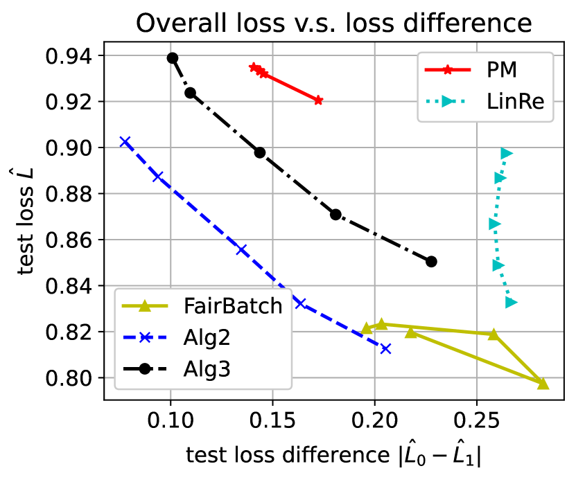
Figure 1: Trade-off between overall MSE and unfairness. A lower curve implies a better trade-off.

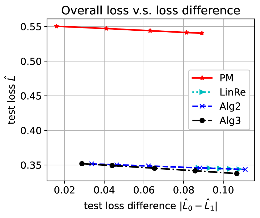
Figure 2: Trade-off between overall BCE and unfairness. A lower curve implies a better trade-off.

Table 1: Linear regression model under EL fairness. The loss function in this example is the mean squared error loss.

		$\gamma=0$	$\gamma=0.1$
	test loss	$0.9246\pm 0.0083$	$0.9332\pm 0.0101$
PM	test $|\hat{L}_{0}-\hat{L}_{1}|$	$0.1620\pm 0.0802$	$0.1438\pm 0.0914$
	test loss	$0.9086\pm 0.0190$	$0.8668\pm 0.0164$
LinRe	test $|\hat{L}_{0}-\hat{L}_{1}|$	$0.2687\pm 0.0588$	$0.2587\pm 0.0704$
	test loss	$0.8119\pm 0.0316$	$0.8610\pm 0.0884$
Fair  Batch	test $|\hat{L}_{0}-\hat{L}_{1}|$	$0.2862\pm 0.1933$	$0.2708\pm 0.1526$
	test loss	${0.9186}\pm{0.0179}$	${0.8556}\pm{0.0217}$
ours Alg 2	test $|\hat{L}_{0}-\hat{L}_{1}|$	$0.0699\pm 0.0469$	$0.1346\pm 0.0749$
	test loss	$0.9522\pm 0.0209$	$0.8977\pm 0.0223$
ours Alg 3	test $|\hat{L}_{0}-\hat{L}_{1}|$	$0.0930\pm 0.0475$	$0.1437\pm 0.0907$

Table 1 illustrates the means and standard deviations of empirical loss and the loss difference between Black and White students. The first row specifies desired fairness level ($\gamma=0$ and $\gamma=0.1$) used as the input to each algorithm. Based on Table 1, when desired fairness level is $\gamma=0$, the model fairness level trained by LinRe and FairBatch method is far from $\gamma=0$. We also realized that the performance of FairBatch highly depends on the random seed. As a result, the fairness level of the model trained by FairBatch has a high variance (0.1933 in this example) in these five independent runs of the experiment, and in some of these runs, it can achieve desired fairness level. This is because the FairBatch algorithm does not come with any performance guarantee, and as stated in (Roh et al., 2020), FairBatch calculates a biased estimate of the gradient in each epoch, and the mini-batch sampling distribution keeps changing from one epoch to another epoch. We observed that FairBatch has better performance with a non-linear model (see Table 3). Both Algorithms 2 and 3 can achieve a fairness level close to $\gamma=0$. However, Algorithm 3 finds a sub-optimal solution and achieves higher MSE compared to Algorithm 2. For $\gamma=0.1$, in addition to Algorithms 2 and 3, the penalty method also achieves a fairness level close to desired fairness level $\gamma=0.1$ (i.e., $|\hat{L}_{1}-\hat{L}_{0}|=0.0892$). Algorithm 2 still achieves the lowest MSE compared to Algorithm 3 and the penalty method. The model trained by FairBatch also suffers from high variance in the fairness level. We want to emphasize that even though Algorithm 3 has a higher MSE compared to Algorithm 2, it is much faster, as stated in Section 3.

We also investigate the trade-off between fairness and overall loss under different algorithms. Figure 2 illustrates the MSE loss as a function of the loss difference between Black and White students. Specifically, we run Algorithm 2, Algorithm 3, and the baselines under different values of $\gamma=[0.0250,0.05,0.1,0.15,0.2]$. For each $\gamma$, we repeat the experiment five times and calculate the average MSE and average MSE difference over these five runs using the test dataset. Figure 2 shows the penalty method, linear relaxation, and FairBatch are not sensitive to input $\gamma$. However, Algorithm 2 and Algorithm 3 are sensitive to $\gamma$; As $\gamma$ increases, $|\hat{L}_{0}(\boldsymbol{w}^{*})-\hat{L}_{1}(\boldsymbol{w}^{*})|$ increases and MSE decreases.

Logistic Regression and Adult Income Dataset. We consider the adult income dataset containing the information of 48,842 individuals (Kohavi, 1996). Each data point consists of 14 features, including age, education, race, etc. In this study, we consider race (White or Black) as the sensitive attribute and denote the White demographic group by $A=0$ and the Black group by $A=1$. We first pre-process the dataset by removing the data points with a missing value or with a race other than Black and White; this results in 41,961 data points. Among these data points, 4585 belong to the Black group. For each data point, we convert all the categorical features to one-hot vectors with $110$ dimension and randomly split the dataset into training and test data sets (70% of the dataset is used for training). The goal is to predict whether the income of an individual is above $\$50K$ using a $\gamma$-EL fair logistic regression model. In this experiment, we solve optimization problem (11), with $\hat{L}$ and $\hat{L}_{a}$ being the overall and the group specific empirical average of binary cross entropy (BCE) loss, respectively.

Table 2: Logistic Regression model under EL fairness. The loss function in this example is binary cross entropy loss.

		$\gamma=0$	$\gamma=0.1$
	test loss	$0.5594\pm 0.0101$	$0.5404\pm 0.0046$
PM	test $|\hat{L}_{0}-\hat{L}_{1}|$	$0.0091\pm 0.0067$	$0.0892\pm 0.0378$
	test loss	$0.3468\pm 0.0013$	$0.3441\pm 0.0012$
LinRe	test $|\hat{L}_{0}-\hat{L}_{1}|$	$0.0815\pm 0.0098$	$0.1080\pm 0.0098$
	test loss	$1.5716\pm 0.8071$	$1.2116\pm 0.8819$
Fair  Batch	test $|\hat{L}_{0}-\hat{L}_{1}|$	$0.6191\pm 0.5459$	$0.3815\pm 0.3470$
	test loss	${0.3516}\pm{0.0015}$	$0.3435\pm 0.0012$
Ours Alg2	test $|\hat{L}_{0}-\hat{L}_{1}|$	$0.0336\pm 0.0075$	$0.1110\pm 0.0140$
	test loss	$0.3521\pm 0.0015$	${0.3377}\pm 0.0015$
Ours Alg3	test $|\hat{L}_{0}-\hat{L}_{1}|$	$0.0278\pm 0.0075$	$0.1068\pm 0.0138$

The comparison of Algorithm 2, Algorithm 3, and the baselines is shown in Table 2, where we conduct five independent runs of experiments, and calculate the mean and standard deviation of overall loss and the loss difference between two demographic groups. The first row in this table shows the value of $\gamma$ used as an input to the algorithms. The results show that linear relaxation, algorithm 2 and Algorithm 3 have very similar performances. All of these three algorithms are able to satisfy the $\gamma$-EL with small test loss. Similar to Table 1, we observe the high variance in the performance of FairBatch, which highly depends on the random seed.

In Figure 2, we compare the performance-fairness trade-off. We focus on binary cross entropy on the test dataset. To generate this figure, we run Algorithm 2, Algorithm 3, and the baselines (we do not include the curve for FairBatch due to large overall loss and high variance in performance) under different values of $\gamma=[0.02,0.04,0.06,0.08,0.1]$ for five times and calculate the average BCE and the average BCE difference. We observe Algorithms 2 and 3 and the linear relaxation have a similar trade-off between $\hat{L}$ and $|\hat{L}_{0}-\hat{L}_{1}|$.

Experiment with a non-linear model

We repeat our first experiment with nonlinear models to demonstrate how we can use our algorithms to fine-tune a non-linear model. We work with the Law School Admission dataset, and we train a neural network with one hidden layer which consists of 125 neurons. We use sigmoid as the activation function for the hidden layer. We run the following algorithms,

• Penalty Method: We solve optimization problem (10). In this example, $\hat{L}$ and $\hat{L}_{a}$ are not convex anymore. The hyperparameters except for the learning rate remain the same as in the first experiment. The learning rate is set to be $0.001$.

• FairBatch: we train the whole network using FairBatch with mini-batch Adam optimization with a batch size of 100 and a learning rate of $0.001$.

• Linear Relaxation: In order to take advantage of CVXPY, first, we train the network without any fairness constraint using batch Adam optimization (i.e., the batch size is equal to the size of the training dataset) with a learning rate of $0.001$. Then, we fine-tune the parameters of the output layer. Note that the output layer has 126 parameters, and we fine-tune those under relaxed EL fairness. In particular, we solve problem (9) after linear relaxation.

• Algorithm 2 and Algorithm 3: We can run Algorithm 2 and Algorithm 3 to fine-tune the neural network. After training the network without any constraint using batch Adam optimization, we solve (9) using Algorithm 2 and Algorithm 3.

Table 3 illustrates the average and standard deviation of empirical loss and the loss difference between Black and White students. Both Algorithm 2 and Algorithm 3 can achieve a fairness level (i.e., $|\hat{L}_{0}-\hat{L}_{1}|$) close to desired fairness level $\gamma$. Also, we can see that the MSE of Algorithm 2 and Algorithm 3 under the nonlinear model is slightly lower than the MSE under the linear model.

We also investigate how MSE $\hat{L}$ changes as a function of fairness level $|\hat{L}_{1}-\hat{L}_{0}|$. Figure 3 illustrates the MSE-fairness trade-off. To generate this plot, we repeat the experiment for $\gamma=[0.025,0.05,0.1,0.15,0.2]$. For each $\gamma$, we ran the experiment 5 times and calculated the average of MSE $\hat{L}$ and the average of MSE difference using the test dataset. Based on Figure 3, we observe that FairBatch and LinRe are not very sensitive to the input $\gamma$. However, FairBatch may sometimes show a better trade-off than Algorithm 2. In this example, PM, Algorithm 2, and Algorithm 3 are very sensitive to $\gamma$, and as $\gamma$ increases, MSE $\hat{L}$ decreases and $|\hat{L}_{0}-\hat{L}_{1}|$ increases.

Table 3: Neural Network training under EL fairness. The loss function in this example is the mean squared error loss.

		$\gamma=0$	$\gamma=0.1$
	test loss	$0.9490\pm 0.0584$	$0.9048\pm 0.0355$
PM	test $|\hat{L}_{0}-\hat{L}_{1}|$	$0.1464\pm 0.1055$	$0.1591\pm 0.0847$
	test loss	$0.8489\pm 0.0195$	$0.8235\pm 0.0165$
LinRe	test $|\hat{L}_{0}-\hat{L}_{1}|$	$0.6543\pm 0.0322$	$0.5595\pm 0.0482$
	test loss	$0.9012\pm 0.1918$	$0.8638\pm 0.0863$
Fair  Batch	test $|\hat{L}_{0}-\hat{L}_{1}|$	$0.2771\pm 0.1252$	$0.1491\pm 0.0928$
	test loss	$0.9117\pm 0.0172$	$0.8519\pm 0.0195$
ours Alg 2	test $|\hat{L}_{0}-\hat{L}_{1}|$	$0.0761\pm 0.0498$	$0.1454\pm 0.0749$
	test loss	$0.9427\pm 0.0190$	$0.8908\pm 0.0209$
ours Alg 3	test $|\hat{L}_{0}-\hat{L}_{1}|$	$0.0862\pm 0.0555$	$0.1423\pm 0.0867$

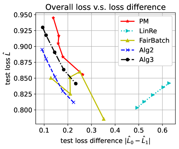
Figure 3: Trade-off between overall MSE and unfairness. A lower curve implies a better trade-off.

Limitation and Negative Societal Impact. 1) Our theoretical guarantees are valid under the stated assumptions (e.g., the convexity of $L({\boldsymbol{w}})$, i.i.d. samples, binary sensitive attribute). These assumptions have been clearly stated throughout this paper. 2) In this paper, we develop an algorithm for finding a fair predictor under EL fairness. However, we do not claim this notion is better than other fairness notions. Depending on the scenario, this notion may or may not be suitable for mitigating unfairness.

7 Conclusion

In this work, we studied supervised learning problems under the Equalized Loss (EL) fairness (Zhang et al., 2019), a notion that requires the expected loss to be balanced across different demographic groups. By imposing the EL constraint, the learning problem can be formulated as a non-convex problem. We proposed two algorithms with theoretical performance guarantees to find the global optimal and a sub-optimal solution to this non-convex problem.

Appendix A Appendix

A.1 Some notes on the code for reproducibility

In this part, we provide a description of the files provided in our GitHub repository.

• $law\_data.py$: This file includes a function called $law\_data(seed)$ which processes the law school admission dataset and splits the dataset randomly into training and test datasets (we keep 70% of the datapoints for training). Later, in our experiments, we set the $seed$ equal to 0, 1, 2, 3, and 4 to get five different splits to repeat our experiments five times.

• $Adult\_data.py$: This file includes a function called $Adult\_dataset(seed)$ which processes the adult income dataset and splits the dataset randomly into training and test datasets. Later, in our experiments, we set the $seed$ equal to 0, 1, 2, 3, 4 to get five different splits to repeat our experiments five times.

• $Algorithms.py$: This file includes the following functions,

  • $ELminimizer(X0,Y0,X1,Y1,gamma,eta,model)$: This function implements Elminimizer algorithm. $(X0,Y0)$ are the training datapoints belonging to group $A=0$ and $(X1,Y1)$ are the datapoits belonging to group $A=1$. $gamma$ is the fairness level for EL constraint. $\eta$ is the reqularizer parameter (in our experiments, $\eta=0.002$). $model$ determines the model that we want to train. If $model="linear"$, then we train a linear regression model. If $model="logistic"$, then we train a logisitic regression model. This function returns five variables $(w,b,l0,l1,l)$. $w,b$ are the weight vector and bias term of the trained model. $l_{0},l_{1}$ are the average training loss of group 0 and group 1, respectively. $l$ is the overall training loss.

  • $Algorithm2(X0,Y0,X1,Y1,gamma,eta,model)$: This function implements Algorithm 2 which calls Elminimizer algorithm twice. This function also returns five variables $(w,b,l0,l1,l)$. These variables have been defined above.

  • $Algorithm3(X0,Y0,X1,Y1,gamma,eta,model)$: This function implements Algorithm 3 which finds a sub-optimal solution under EL fairness. This function also returns five variables $(w,b,l0,l1,l)$. These variables have been defined above.

  • $solve\_constrained\_opt(X0,Y0,X1,Y1,eta,landa,model)$: This function uses the CVXPY package to solve the optimization problem (4). We set $landa$ equal to $\lambda_{mid}^{(i)}$ to solve the optimization problem (4) in iteration $i$ of Algorithm 1.

  • $calculate\_loss(w,b,X0,Y0,X1,Y1,model)$: This function is used to find the test loss. $w,b$ are model parameters (trained by Algorithm 2 or 3). It returns the average loss of group 0 and group 1 and the overall loss based on the given dataset.

  • $solve\_lin\_constrained\_opt(X0,Y0,X1,Y1,gamma,eta,model)$: This function is for solving optimization problem (8) after linear relaxation.

• $Baseline.py$: this file includes the following functions,

  • $penalty\_method(method,X\_0,y\_0,X\_1,y\_1,num\_itr,lr,r,gamma,seed,epsilon)$ where $method$ can be either $"linear"$ for linear regression or $"logistic"$ for logistic regression. This function uses the penalty method and trains the model under EL using the Adam optimization. $num\_itr$ is the maximum number of iterations. $r$ is the regularization parameter (it is set to $0.002$ in our experiment). $lr$ is the learning rate and $gamma$ is the fairness level. $\epsilon$ is used for the stopping criterion. This function returns the trained model (which is a torch module), and training loss of group 0 and group 1, and the overall training loss.

  • $fair\_batch(method,X\_0,y\_0,X\_1,y\_1,num\_itr,lr,r,alpha,gamma,seed,epsilon)$: This function is used to simulate the FairBatch algorithm [Roh et al., 2020]. The input parameters are similar to the input parameters of $penalty\_method$ except for $alpha$. This parameter determines how to adjust the sub-sampling distribution for mini-batch formation. Please look at the next section for more details. This function returns the trained model (which is a torch module), and training loss of group 0 and group 1, and the overall training loss.

$table1\_2.py$ uses the above functions to reproduce the results in Table 1 and Table 2. $figure1\_2.py$ uses the above functions to reproduce Figure 1 and Figure 2. We provide some comments in these files to make the code more readable. We have also provided code for training non-linear models. Please use $Table3.py$ and $figure3.py$ to generate the results in Table 3 and Figure 3, respectively.

Lastly, use the following command to generate results in Table 1:

• python3 table1_2.py --experiment=1 --gamma=0.0

• python3 table1_2.py --experiment=1 --gamma=0.1

Use the following command to generate results in Table 2:

• python3 table1_2.py --experiment=2 --gamma=0.0

• python3 table1_2.py --experiment=2 --gamma=0.1

Use the following command to generate results in Table 3:

• python3 table3.py --gamma=0.0

• python3 table3.py --gamma=0.1

Use the following command to generate results in Figure 1:

• python3 figure1_2.py --experiment=1

Use the following command to generate results in Figure 2:

• python3 figure1_2.py --experiment=2

Use the following command to generate results in Figure 3:

• python3 figure3.py

Note that you need to install packages in requirements.txt

A.2 Notes on FairBatch [Roh et al., 2020]

This method has been proposed to find a predictor under equal opportunity, equalized odd or statistical parity. In each epoch, this method identifies the disadvantaged group and increases the subsampling rate corresponding to the disadvantaged group in mini-batch selection for the next epoch. We modify this approach for $\gamma$-EL as follows,

• We initialize the sub-sampling rate of group $a$ (denoted by $SR^{(0)}_{a}$) for mini-batch formation by $SR^{(0)}_{a}=\frac{n_{a}}{n},a=0,1$. We Form the mini-batches using $SR^{(0)}_{0}$ and $SR^{(0)}_{1}$.

• At epoch $i$, we run gradient descent using the mini-batches formed by $SR^{(i-1)}_{0}$ and $SR^{(i-1)}_{1}$, and we obtain new model parameters $\boldsymbol{w}_{i}$.

• After epoch $i$, we calculate the empirical loss of each group. Then, we update $SR^{(i)}_{a}$ as follows,

  $$SR^{(i)}_{a}\longleftarrow SR^{(i-1)}_{a}+\alpha \mbox{if }\hat{L}_{a}(\boldsymbol{w}_{i})-\hat{L}_{1-a}(\boldsymbol{w}_{i})>\gamma$$

  $$SR^{(i)}_{a}\longleftarrow SR^{(i-1)}_{a}-\alpha \mbox{if }\hat{L}_{a}(\boldsymbol{w}_{i})-\hat{L}_{1-a}(\boldsymbol{w}_{i})<-\gamma$$

  $$SR^{(i)}_{a}\longleftarrow SR^{(i-1)}_{a} \mbox{o.w.},$$

  where is $\alpha$ is a hyperparameter and, in our experiment, is equal to $0.005$.

A.3 Details of numerical experiments and additional numerical results

Due to the space limits of the main paper, we provide more details on our experiments here,

• Stopping criteria for penalty method and FairBatch: For stopping criteria, we stopped the learning process when the change in the objective function is less than $10^{-6}$ between two consecutive epochs. The reason that we used $10^{-6}$ was that we did not observe any significant change by choosing a smaller value.

• Learning rate for penalty method and FairBatch: We chose $0.005$ for the learning rate for training a linear model. For the experiment with a non-linear model, we set the learning rate to be $0.001$.

• Stopping criteria for Algorithm 2 and Algorithm 3: As we stated in the main paper, we set $\epsilon=0.01$ in ELminimizer and Algorithm 3. Choosing smaller $\epsilon$ did not change the performance significantly.

• Linear Relaxation: Note that equation (8) after linear relaxation is a convex optimization problem. We directly solve this optimization problem using CVXPY.

The experiment has been done on a system with the following configurations: 24 GB of RAM, 2 cores of P100-16GB GPU, and 2 cores of Intel Xeon CPU@2.3 GHz processor. We used GPUs for training FairBatch.

A.4 Notes on the Reduction Approach [Agarwal et al., 2018, 2019]

Let $Q(f)$ be a distribution over $\mathcal{F}$. In order to find optimal $Q(f)$ using the reduction approach, we have to solve the following optimization problem,

$$\min_{Q} \sum_{f\in\mathcal{F}}Q(f)\mathbb{E}\{l(Y,f(\boldsymbol{X}))\}$$

$$s.t., \sum_{f\in\mathcal{F}}Q(f)\mathbb{E}\{l(Y,f(\boldsymbol{X}))|A=0\}=\sum_{f\in\mathcal{F}}Q(f)\mathbb{E}\{l(Y,f(\boldsymbol{X}))\}$$

$$\sum_{f\in\mathcal{F}}Q(f)\mathbb{E}\{l(Y,f(\boldsymbol{X}))|A=1\}=\sum_{f\in\mathcal{F}}Q(f)\mathbb{E}\{l(Y,f(\boldsymbol{X}))\}$$

Similar to [Agarwal et al., 2018, 2019], we can re-write the above optimization problem in the following form,

$$\min_{Q} \sum_{f\in\mathcal{F}}Q(f)\mathbb{E}\{l(Y,f(\boldsymbol{X}))\}$$

$$s.t., \sum_{f\in\mathcal{F}}Q(f)\mathbb{E}\{l(Y,f(\boldsymbol{X}))|A=0\}-\sum_{f\in\mathcal{F}}Q(f)\mathbb{E}\{l(Y,f(\boldsymbol{X}))\}\leq 0$$

$$-\sum_{f\in\mathcal{F}}Q(f)\mathbb{E}\{l(Y,f(\boldsymbol{X}))|A=0\}+\sum_{f\in\mathcal{F}}Q(f)\mathbb{E}\{l(Y,f(\boldsymbol{X}))\}\leq 0$$

$$\sum_{f\in\mathcal{F}}Q(f)\mathbb{E}\{l(Y,f(\boldsymbol{X}))|A=1\}-\sum_{f\in\mathcal{F}}Q(f)\mathbb{E}\{l(Y,f(\boldsymbol{X}))\}\leq 0$$

$$-\sum_{f\in\mathcal{F}}Q(f)\mathbb{E}\{l(Y,f(\boldsymbol{X}))|A=1\}+\sum_{f\in\mathcal{F}}Q(f)\mathbb{E}\{l(Y,f(\boldsymbol{X}))\}\leq 0$$

Then, the reduction approach forms the Lagrangian function as follows,

$$L(Q,\mu) = \sum_{f\in\mathcal{F}}Q(f)\mathbb{E}\{l(Y,f(\boldsymbol{X}))\}$$

$$- \mu_{1}\cdot\left(\sum_{f\in\mathcal{F}}Q(f)\mathbb{E}\{l(Y,f(\boldsymbol{X}))|A=0\}-\sum_{f\in\mathcal{F}}Q(f)\mathbb{E}\{l(Y,f(\boldsymbol{X}))\}\right)$$

$$- \mu_{2}\cdot\left(-\sum_{f\in\mathcal{F}}Q(f)\mathbb{E}\{l(Y,f(\boldsymbol{X}))|A=0\}+\sum_{f\in\mathcal{F}}Q(f)\mathbb{E}\{l(Y,f(\boldsymbol{X}))\}\right)$$

$$- \mu_{3}\cdot\left(\sum_{f\in\mathcal{F}}Q(f)\mathbb{E}\{l(Y,f(\boldsymbol{X}))|A=1\}-\sum_{f\in\mathcal{F}}Q(f)\mathbb{E}\{l(Y,f(\boldsymbol{X}))\}\right)$$

$$- \mu_{4}\cdot\left(-\sum_{f\in\mathcal{F}}Q(f)\mathbb{E}\{l(Y,f(\boldsymbol{X}))|A=1\}+\sum_{f\in\mathcal{F}}Q(f)\mathbb{E}\{l(Y,f(\boldsymbol{X}))\}\right),$$

$$\mu_{1}\geq 0,\mu_{2}\geq 0,\mu_{3}\geq 0,\mu_{4}\geq 0.$$

Since $f$ is parametrized with $\boldsymbol{w}$, we can find distribution $Q(\boldsymbol{w})$ over $\mathbb{R}^{d_{\boldsymbol{w}}}$. Therefore, we rewrite the problem in the following form,

$$L(Q(\boldsymbol{w}),\mu_{1},\mu_{2},\mu_{3},\mu_{4}) = \sum_{\boldsymbol{w}}Q({\boldsymbol{w}})L({\boldsymbol{w}})$$

$$- \mu_{1}\left(\sum_{{\boldsymbol{w}}}Q(\boldsymbol{w})L_{0}({\boldsymbol{w}})-\sum_{{\boldsymbol{w}}}Q(\boldsymbol{w})L({\boldsymbol{w}})\right)$$

$$- \mu_{2}\left(-\sum_{{\boldsymbol{w}}}Q(\boldsymbol{w})L_{0}({\boldsymbol{w}})+\sum_{{\boldsymbol{w}}}Q(\boldsymbol{w})L({\boldsymbol{w}})\right)$$

$$- \mu_{3}\left(\sum_{{\boldsymbol{w}}}Q(\boldsymbol{w})L_{1}({\boldsymbol{w}})-\sum_{{\boldsymbol{w}}}Q(\boldsymbol{w})L({\boldsymbol{w}})\right)$$

$$- \mu_{4}\left(-\sum_{{\boldsymbol{w}}}Q(\boldsymbol{w})L_{1}({\boldsymbol{w}})+\sum_{{\boldsymbol{w}}}Q(\boldsymbol{w})L({\boldsymbol{w}})\right)$$

The reduction approach updates $Q({\boldsymbol{w}})$ and $(\mu_{1},\mu_{2},\mu_{3},\mu_{4})$ alternatively. Looking carefully at Algorithm 1 in [Agarwal et al., 2018], after updating $(\mu_{1},\mu_{2},\mu_{3},\mu_{4})$, we need to have access to an oracle that is able to solve the following optimization problem in each iteration,

$$\min_{{\boldsymbol{w}}}(1+\mu_{1}-\mu_{2}+\mu_{3}-\mu_{4})L({\boldsymbol{w}})+(-\mu_{1}+\mu_{2})L_{0}(\boldsymbol{w})+(-\mu_{3}+\mu_{4})L_{1}({\boldsymbol{w}})$$

The above optimization problem is not convex for all $\mu_{1},\mu_{2},\mu_{3},\mu_{4}$. Therefore, in order to use the reduction approach, we need to have access to an oracle that is able to solve the above non-convex optimization problem which is not available. Note that the original problem (1) is a non-convex optimization problem and using the reduction approach just leads to another non-convex optimization problem.

A.5 Equalized Loss & Bounded Group Loss

In this section, we study the relation between EL and BGL fairness notions. It is straightforward to see that any predictor satisfying $\gamma$-BGL also satisfies the $\gamma$-EL. However, it is unclear to what extend an optimal fair predictor under $\gamma$-EL satisfies the BGL fairness notion. Next, we theoretically study the relation between BGL and EL fairness notions.

Let $\boldsymbol{w}^{*}$ be denoted as the solution to (1) and $f_{\boldsymbol{w}^{*}}$ the corresponding optimal $\gamma$-EL fair predictor. Theorem A.1 below shows that under certain conditions, it is impossible for both groups to experience a loss larger than $2\gamma$ under the optimal $\gamma$-EL fair predictor.

Theorem A.1.

Suppose there exists a predictor that satisfies $\gamma$-BGL fairness notion. That is, the following optimization problem has at least one feasible point.

$$\min_{\boldsymbol{w}}~{}~{}L(\boldsymbol{w})\text{ s.t.}~{}~{}L_{a}(\boldsymbol{w})\leq\gamma,~{}\forall a\in\{0,1\}.$$ (12)

Then, the followings hold,

$$\min\{L_{0}(\boldsymbol{w}^{*}),L_{1}(\boldsymbol{w}^{*})\} \leq \gamma;$$

$$\max\{L_{0}(\boldsymbol{w}^{*}),L_{1}(\boldsymbol{w}^{*})\} \leq 2\gamma.$$

Theorem A.1 shows that $\gamma$-EL implies $2\gamma$-BGL if $\gamma$-BGL is a feasible constraint. Therefore, if $\gamma$ is not too small (e.g., $\gamma=0$), then EL and BGL are not contradicting each other.

We emphasize that we are not claiming that whether EL fairness is better than BGL. Instead, these relations indicate the impacts the two fairness constraints could have on the model performance; the results may further provide the guidance for policy-makers.

A.6 Proofs

In order to prove Theorem 3.3, we first introduce two lemmas.

Lemma A.2.

Under assumption 3.2, there exists $\overline{\boldsymbol{w}}\in\mathbb{R}^{d_{\boldsymbol{w}}}$ such that $L_{0}(\overline{\boldsymbol{w}})=L_{1}(\overline{\boldsymbol{w}})=L(\overline{\boldsymbol{w}})$ and $\lambda^{(0)}_{start}\leq L(\overline{\boldsymbol{w}})\leq\lambda^{(0)}_{end}$.

Proof. Let $q_{0}(\beta)=L_{0}((1-\beta)\boldsymbol{w}_{G_{0}}+\beta\boldsymbol{w}_{G_{1}})$ and $q_{1}(\beta)=L_{1}((1-\beta)\boldsymbol{w}_{G_{0}}+\beta\boldsymbol{w}_{G_{1}})$, and $q(\beta)=q_{0}(\beta)-q_{1}(\beta),\beta\in[0,1]$. Note that $\nabla_{\boldsymbol{w}}L_{a}(\boldsymbol{w}_{G_{a}})=0$ because $\boldsymbol{w}_{G_{a}}$ is the minimizer of $L_{a}(\boldsymbol{w})$.

First, we show that $L_{0}((1-\beta)\boldsymbol{w}_{G_{0}}+\beta\boldsymbol{w}_{G_{1}})$ is an increasing function in $\beta$, and $L_{1}((1-\beta)\boldsymbol{w}_{G_{0}}+\beta\boldsymbol{w}_{G_{1}})$ is a decreasing function in $\beta$. Note that $q^{\prime}_{0}(0)=(\boldsymbol{w}_{G_{1}}-\boldsymbol{w}_{G_{0}})^{T}\nabla_{\boldsymbol{w}}L_{0}(\boldsymbol{w}_{G_{0}})=0$, and $q_{0}(\beta)$ is convex because $L_{0}(\boldsymbol{w})$ is convex. This implies that $q^{\prime}(\beta)$ is an increasing function, and $q^{\prime}_{0}(\beta)\geq 0,\forall\beta\in[0,1]$. Similarly, we can show that $q^{\prime}_{1}(\beta)\leq 0,\forall\beta\in[0,1]$.

Note that under Assumption (3.2), $q(0)<0$ and $q(1)>0$. Therefore, by the intermediate value theorem, the exists $\overline{\beta}\in(0,1)$ such that $q(\overline{\beta})=0$. Define $\overline{\boldsymbol{w}}=(1-\overline{\beta})\boldsymbol{w}_{G_{0}}+\overline{\beta}\boldsymbol{w}_{G_{1}}$. We have,

$$q(\overline{\beta}) = 0\implies L_{0}(\overline{\boldsymbol{w}})=L_{1}(\overline{\boldsymbol{w}})=L(\overline{\boldsymbol{w}})$$

$$\boldsymbol{w}_{G_{0}} \mbox{minimizer of }L_{0}\implies$$ is

$$L(\overline{\boldsymbol{w}}) = L_{0}(\overline{\boldsymbol{w}})\geq\lambda^{(0)}_{start}$$

$$q^{\prime}_{0}(\beta) \geq 0,\forall\beta\in[0,1]\implies q_{0}(1)\geq q_{0}(\overline{\beta})\implies$$

$$\lambda_{end}^{(0)} \geq L_{0}(\overline{\boldsymbol{w}})=L(\overline{\boldsymbol{w}})$$

Lemma A.3.

$L_{0}(\boldsymbol{w}_{i}^{*})=\lambda_{mid}^{(i)}$, where $\boldsymbol{w}_{i}^{*}$ is the solution to (4).

Proof. We proceed by contradiction. Assume that $L_{0}(\boldsymbol{w}_{i}^{*})<\lambda_{mid}^{(i)}$ (i.e., $\boldsymbol{w}_{i}^{*}$ is an interior point of the feasible set of (4)). Notice that $\boldsymbol{w}_{G_{1}}$ cannot be in the feasible set of (4) because $L_{0}(\boldsymbol{w}_{G_{1}})=\lambda_{end}^{(0)}>\lambda_{mid}^{(i)}$. As a result, $\nabla_{\boldsymbol{w}}L_{1}(\boldsymbol{w}_{i}^{*})\neq 0$. This is a contradiction because $\boldsymbol{w}_{i}^{*}$ is an interior point of the feasible set of a convex optimization and cannot be optimal if $\nabla_{\boldsymbol{w}}L_{1}(\boldsymbol{w}_{i}^{*})$ is not equal to zero.

Proof [Theorem 3.3]

Now, we show that $L(\boldsymbol{w}^{*})\in I_{i}$ for all $i$ ($\boldsymbol{w}^{*}$ is the solution to (1) when $\gamma=0$. As a result, $L_{0}(\boldsymbol{w}^{*})=L_{1}(\boldsymbol{w}^{*})=L(\boldsymbol{w}^{*})$). Note that $L(\boldsymbol{w}^{*})=L_{0}(\boldsymbol{w}^{*})\geq\lambda_{start}^{(0)}$ because $\boldsymbol{w}_{G_{0}}$ is the minimizer of $L_{0}$. Moreover, $\lambda_{end}^{(0)}\geq L(\boldsymbol{w}^{*})$ otherwise $L(\overline{\boldsymbol{w}})<L(\boldsymbol{w}^{*})$ ($\overline{\boldsymbol{w}}$ is defined in Lemma A.2) and $\boldsymbol{w}^{*}$ is not optimal solution under 0-EL. Therefore, $L(\boldsymbol{w}^{*})\in I_{0}$.

Now we proceed by induction. Suppose $L(\boldsymbol{w}^{*})\in I_{i}$. We show that $L(\boldsymbol{w}^{*})\in I_{i+1}$ as well. We consider two cases.

• $L(\boldsymbol{w}^{*})\leq\lambda_{mid}^{(i)}$. In this case $\boldsymbol{w}^{*}$ is a feasible point for (4), and $L_{1}(\boldsymbol{w}_{i}^{*})=\lambda^{(i)}\leq L_{1}(\boldsymbol{w}^{*})=L(\boldsymbol{w}^{*})\leq\lambda_{mid}^{(i)}$. Therefore, $L(\boldsymbol{w}^{*})\in I_{i+1}$.

• $L(\boldsymbol{w}^{*})>\lambda_{mid}^{(i)}$. In this case, we proceed by contradiction to show that $\lambda^{(i)}\geq\lambda_{mid}^{(i)}$. Assume that $\lambda^{(i)}<\lambda_{mid}^{(i)}$. Define $r(\beta)=r_{0}(\beta)-r_{1}(\beta)$, where $r_{a}(\beta)=L_{a}((1-\beta)\boldsymbol{w}_{G_{0}}+\beta\boldsymbol{w}_{i}^{*})$. Note that $\lambda^{(i)}=r_{1}(1)$ By Lemma A.3, $r_{0}(1)=\lambda_{mid}^{(i)}$. Therefore, $r(1)=\lambda_{mid}^{(i)}-\lambda^{(i)}>0$. Moreover, under Assumption 3.2, $r(0)<0$. Therefore, by the intermediate value theorem, there exists $\overline{\beta}_{0}\in(0,1)$ such that $r(\overline{\beta}_{0})=0$. Similar to the proof of Lemma A.2, we can show that $r_{0}(\beta)$ in an increasing function for all $\beta\in[0,1]$. As a result $r_{0}(\overline{\beta}_{0})<r_{0}(1)=\lambda_{mid}^{(i)}$. Define $\overline{\boldsymbol{w}}_{0}=(1-\overline{\beta}_{0})\boldsymbol{w}_{G_{0}}+\overline{\beta}_{0}\boldsymbol{w}_{i}^{*}$. We have,

  $$r_{0}(\overline{\beta}_{0})=L_{0}(\overline{\boldsymbol{w}}_{0})=L_{1}(\overline{\boldsymbol{w}}_{0})=L(\overline{\boldsymbol{w}}_{0})<\lambda_{mid}^{(i)}$$ (13)

  $$L(\boldsymbol{w}^{*})>\lambda_{mid}^{(i)}$$ (14)

  The last two equations imply that $\boldsymbol{w}^{*}$ is not a global optimal fair solution under $0$-EL fairness constraint and it is not the global optmal solution to (1). This is a contradiction. Therefore, if $L(\boldsymbol{w}^{*})>\lambda_{mid}^{(i)}$, then $\lambda^{(i)}\geq\lambda_{mid}^{(i)}$. As a result, $L(\boldsymbol{w}^{*})\in I_{i+1}$

By two above cases and the nested interval theorem, we conclude that,

$$L(\boldsymbol{w}^{*})\in\cap_{i=1}^{\infty}I_{i},~{}\lim_{i\to\infty}\lambda_{mid}^{(i)}=L(\boldsymbol{w}^{*}),$$

$$\mbox{define}\lambda_{mid}^{\infty}:=\lim_{i\to\infty}\lambda_{mid}^{(i)}$$

Therefore, $\lim_{i\to\infty}\boldsymbol{w}_{i}^{*}$ would be the solution to the following optimziation problem,

$$\arg\min_{\boldsymbol{w}}L_{1}(\boldsymbol{w})s.t.,L_{0}(\boldsymbol{w})\leq\lambda_{mid}^{\infty}=L(\boldsymbol{w}^{*})$$

By lemma A.3, the solution to above optimization problem (i.e., $\lim_{i\to\infty}\boldsymbol{w}_{i}^{*}$) satisfies the following, $L_{0}(\lim_{i\to\infty}\boldsymbol{w}_{i}^{*})=\lambda_{mid}^{\infty}=L(\boldsymbol{w}^{*})$. Therefore, $\lim_{i\to\infty}\boldsymbol{w}_{i}^{*}$ is the global optimal solution to optimization problem (1).

Proof [Theorem 3.4 ] Let’s assume that $\boldsymbol{w}_{O}$ does not satisfy the $\gamma$-EL. Let $\boldsymbol{w}^{*}$ be the optimal weight vector under $\gamma$-EL. It is clear that $\boldsymbol{w}^{*}\neq\boldsymbol{w}_{O}$.

Step 1. we show that one of the following holds,

$$L_{0}(\boldsymbol{w}^{*})-L_{1}(\boldsymbol{w}^{*})=\gamma$$ (15)

$$L_{0}(\boldsymbol{w}^{*})-L_{1}(\boldsymbol{w}^{*})=-\gamma$$ (16)

Proof by contradiction. Assume $-\gamma<L_{0}(\boldsymbol{w}^{*})-L_{1}(\boldsymbol{w}^{*})<\gamma$. This implies that $\boldsymbol{w}^{*}$ is an interior point of the feasible set of optimization problem (1). Since $\boldsymbol{w}^{*}\neq\boldsymbol{w}_{O}$, then $\nabla L(\boldsymbol{w}^{*})\neq 0$. As a result, object function of (1) can be improved at $\boldsymbol{w}^{*}$ by moving toward $-\nabla L(\boldsymbol{w}^{*})$. This a contradiction. Therefore, $|L_{0}(\boldsymbol{w}^{*})-L_{1}(\boldsymbol{w}^{*})|=\gamma$.

Step 2. Function $\boldsymbol{w}_{\gamma}=\texttt{ELminimizer}(\boldsymbol{w}_{G_{0}},\boldsymbol{w}_{G_{0}},\epsilon,\gamma)$ is the solution to the following optimization problem,

$$\min_{\boldsymbol{w}}\Pr\{A=0\}L_{0}(\boldsymbol{w})+\Pr\{A=1\}L_{1}(\boldsymbol{w}),$$

$$s.t.,L_{0}(\boldsymbol{w})-L_{1}(\boldsymbol{w})=\gamma$$ (17)

To show the above claim, notice that the solution to optimization problem (A.6) is the same as the following,

$$\min_{\boldsymbol{w}}\Pr\{A=0\}L_{0}(\boldsymbol{w})+\Pr\{A=1\}\tilde{L}_{1}(\boldsymbol{w}),$$

$$s.t.,L_{0}(\boldsymbol{w})-\tilde{L}_{1}(\boldsymbol{w})=0,$$ (18)

where $\tilde{L}_{1}(\boldsymbol{w})=L_{1}(\boldsymbol{w})+\gamma$. Since $L_{0}(\boldsymbol{w}_{G_{0}})-\tilde{L}_{1}(\boldsymbol{w}_{G_{0}})<0$ and $L_{0}(\boldsymbol{w}_{G_{1}})-\tilde{L}_{1}(\boldsymbol{w}_{G_{1}})>0$, by Theorem 3.3, we know that $\boldsymbol{w}_{\gamma}=\texttt{ELminimizer}(\boldsymbol{w}_{G_{0}},\boldsymbol{w}_{G_{0}},\epsilon,\gamma)$ find the solution to (A.6) when $\epsilon$ goes to zero.

Lastly, because $|L_{0}(\boldsymbol{w}^{*})-L_{1}(\boldsymbol{w}^{*})|=\gamma$, we have,

$$\boldsymbol{w}^{*}=\left\{\begin{array}[]{ll}\boldsymbol{w}_{\gamma}&\mbox{if }L(\boldsymbol{w}_{\gamma})\leq L(\boldsymbol{w}_{-\gamma})\\ \boldsymbol{w}_{-\gamma}&\mbox{o.w.}\end{array}\right.$$ (21)

Thus, Algorithm 2 finds the solution to (1).

Proof [Theorem 4.1]

1. Under Assumption 3.2, $g(1)<0$. Moreover, $g(0)\geq 0$. Therefore, by the intermediate value theorem, there exists $\beta_{0}\in[0,1]$ such that $g(\beta_{0})=0$.

2. Since $\boldsymbol{w}_{O}$ is the minimizer of $L(\boldsymbol{w})$, $h^{\prime}(0)=0$. Moreover, since $L(\boldsymbol{w})$ is strictly convex, $h(\beta)$ is strictly convex and $h^{\prime}(\beta)$ is strictly increasing function. As a result, $h^{\prime}(\beta)>0$ for $\beta>0$, and $h(\beta)$ is strictly increasing.

3. Similar to the above argument, $s(\beta)=L_{\hat{a}}((1-\beta)\boldsymbol{w}_{O}+\beta\boldsymbol{w}_{G_{\hat{a}}})$ is strictly decreasing function (notice that $s^{\prime}(1)=0$ and $s(\beta)$ is strictly convex).

   Note that since $h(\beta)=\Pr\{A=\hat{a}\}L_{\hat{a}}((1-\beta)\boldsymbol{w}_{O}+\beta\boldsymbol{w}_{G_{\hat{a}}})+\Pr\{A=1-\hat{a}\}L_{1-\hat{a}}((1-\beta)\boldsymbol{w}_{O}+\beta\boldsymbol{w}_{G_{\hat{a}}})$ is strictly increasing and $L_{\hat{a}}((1-\beta)\boldsymbol{w}_{O}+\beta\boldsymbol{w}_{G_{\hat{a}}})$ is strictly decreasing. Therefore, we conclude that $L_{1-\hat{a}}((1-\beta)\boldsymbol{w}_{O}+\beta\boldsymbol{w}_{G_{\hat{a}}})$ is strictly increasing. As a result, $g(\beta)$ should be strictly decreasing.

Proof [Theorem 4.2] First, we show that if $g_{\gamma}(0)\leq 0$, then $\boldsymbol{w}_{O}$ satisfies $\gamma$-EL.

$$g_{\gamma}(0)\leq 0\implies g(\beta)-\gamma\leq 0\implies L_{\hat{a}}(\boldsymbol{w}_{O})-L_{1-\hat{a}}(\boldsymbol{w}_{O})\leq\gamma$$

Moreover, $L_{\hat{a}}(\boldsymbol{w}_{O})-L_{1-\hat{a}}(\boldsymbol{w}_{O})\geq 0$ because $\hat{a}=\arg\max_{a}L_{a}(\boldsymbol{w}_{O})$. Therefore, $\gamma$-EL is satisfied.

Now, let $g_{\gamma}(0)>0$. Note that under Assumption 3.2, $g_{\gamma}(1)=L_{\hat{a}}(\boldsymbol{w}_{G_{\hat{a}}})-L_{1-\hat{a}}(\boldsymbol{w}_{G_{\hat{a}}})-\gamma<0$. Therefore, by the intermediate value theorem, there exists $\beta_{0}$ such that $g_{\gamma}(\beta_{0})=0$. Moreover, based on Theorem 4.2, $g_{\gamma}$ is a strictly decreasing function. Therefore, the binary search proposed in Algorithm 3 converges to the root of $g_{\gamma}(\beta)$. As a result, $(1-\beta_{mid}^{(\infty)})\boldsymbol{w}_{O}+\beta_{mid}^{(\infty)}\boldsymbol{w}_{G_{\hat{a}}}$ satisfies $\gamma$-EL. Note that since $g(\beta)$ is strictly decreasing, and $g(\beta_{mid}^{(\infty)})=\gamma$, and $\beta^{(\infty)}_{mid}$ is the smallest possible $\beta$ under which $(1-\beta)\boldsymbol{w}_{O}+\beta\boldsymbol{w}_{G_{\hat{a}}}$ satisfies $\gamma$-EL. Since $h$ is increasing, the smallest possible $\beta$ gives us a better accuracy.

Proof [Theorem 4.3] If $g_{\gamma}(0)\leq 0$, then $\boldsymbol{w}_{O}$ satisfies $\gamma$-EL, and $\underline{\boldsymbol{w}}=\boldsymbol{w}_{O}$. In this case, it is easy to see that $L(\boldsymbol{w}_{O})\leq\max_{a\in\{0,1\}}L_{a}(\boldsymbol{w}_{O})$ (because $L(\boldsymbol{w}_{O})$ is a weighted average of $L_{0}(\boldsymbol{w}_{O})$ and $L_{1}(\boldsymbol{w}_{O}))$.

Now assume that $g_{\gamma}(0)>0$. Note that if we prove this theorem for $\gamma=0$, then the theorem will hold for $\gamma>0$. This is because the optimal predictor under $0$-EL satisfies $\gamma$-EL condition as well. In other words, $0$-EL is a stronger constraint than $\gamma$-EL.

Let $\gamma=0$. In this case, Algorithm 3 finds $\underline{\boldsymbol{w}}=(1-\beta_{0})\boldsymbol{w}_{O}+\beta_{0}\boldsymbol{w}_{G_{\hat{a}}}$, where $\beta_{0}$ is defined in Theorem 4.1. We have,

$$(*)~{}~{}g(\beta_{0})=0=L_{\hat{a}}(\underline{\boldsymbol{w}})-L_{1-\hat{a}}(\underline{\boldsymbol{w}})$$

In the proof of theorem 4.1, we showed that $L_{\hat{a}}((1-\beta)\boldsymbol{w}_{O}+\beta\boldsymbol{w}_{G_{\hat{a}}})$ is decreasing in $\beta$. Therefore, we have,

$$(**)~{}~{}L_{\hat{a}}(\underline{\boldsymbol{w}})\leq L_{\hat{a}}(\boldsymbol{w}_{O})$$

Therefore, we have,

$$L(\underline{\boldsymbol{w}}) = \Pr(A=0)\cdot L_{\hat{a}}(\underline{\boldsymbol{w}})+(1-\Pr(A=1))\cdot L_{1-\hat{a}}(\underline{\boldsymbol{w}})$$ (22)

$$(\mbox{By }(*))~{}~{}~{}~{}~{}~{}~{}~{}~{}~{}~{}~{}~{}~{}~{}~{} = L_{\hat{a}}(\underline{\boldsymbol{w}})$$ (23)

$$(\mbox{By }(**))~{}~{}~{}~{}~{}~{}~{}~{}~{}~{}~{}~{}~{}~{}~{} \leq L_{\hat{a}}(\boldsymbol{w}_{O})$$ (24)

Proof [Theorem 4.5]

By the triangle inequality, the following holds,

$$\sup_{f_{\boldsymbol{w}}\in\mathcal{F}}||L_{0}(\boldsymbol{w})-L_{1}(\boldsymbol{w})|-|\hat{L}_{0}(\boldsymbol{w})-\hat{L}_{1}(\boldsymbol{w})||\leq$$ (25)

$$\sup_{f_{\boldsymbol{w}}\in\mathcal{F}}|L_{0}(\boldsymbol{w})-\hat{L}_{0}(\boldsymbol{w})|+\sup_{f_{\boldsymbol{w}}\in\mathcal{F}}|L_{1}(\boldsymbol{w})-\hat{L}_{1}(\boldsymbol{w})|.$$ (26)

Therefore, with probability at least $1-2\delta$ we have,

$$\sup_{f_{\boldsymbol{w}}\in\mathcal{F}}||L_{0}(\boldsymbol{w})-L_{1}(\boldsymbol{w})|-|\hat{L}_{0}(\boldsymbol{w})-\hat{L}_{1}(\boldsymbol{w})||\leq$$

$$B(\delta,n_{0},\mathcal{F})+B(\delta,n_{1},\mathcal{F})$$ (27)

As a result, with probability $1-2\delta$ holds,

$$\{\boldsymbol{w}|f_{\boldsymbol{w}}\in\mathcal{F},|L_{0}(\boldsymbol{w})-L_{1}(\boldsymbol{w})|\leq\gamma\}\subseteq$$

$$\{\boldsymbol{w}|f_{\boldsymbol{w}}\in\mathcal{F},|\hat{L}_{0}(\boldsymbol{w})-\hat{L}_{1}(\boldsymbol{w})|\leq\hat{\gamma}\}$$ (28)

Now consider the following,

$$L(\boldsymbol{\hat{w}})-L(\boldsymbol{w}^{*})=L(\boldsymbol{\hat{w}})-\hat{L}(\boldsymbol{\hat{w}})+\hat{L}(\boldsymbol{\hat{w}})-\hat{L}(\boldsymbol{w}^{*})+\hat{L}(\boldsymbol{w}^{*})-L(\boldsymbol{w}^{*})$$ (29)

By (A.6), $\hat{L}(\boldsymbol{\hat{w}})-\hat{L}(\boldsymbol{w}^{*})\leq 0$ with probability $1-2\delta$. Thus, with probability at least $1-2\delta$, we have,

$$L(\boldsymbol{\hat{w}})-L(\boldsymbol{w}^{*})\leq L(\boldsymbol{\hat{w}})-\hat{L}(\boldsymbol{\hat{w}})+\hat{L}(\boldsymbol{w}^{*})-L(\boldsymbol{w}^{*}).$$ (30)

Therefore, under assumption 4.4, we can conclude with probability at least $1-6\delta$, $L(\boldsymbol{\hat{w}})-L(\boldsymbol{w}^{*})\leq 2B(\delta,n,\mathcal{F})$. In addition, by (A.6), with probability at least $1-2\delta$, we have,

$$|L_{0}(\boldsymbol{\hat{w}})-L_{1}(\boldsymbol{\hat{w}})| \leq B(\delta,n_{0},\mathcal{F})+B(\delta,n_{1},\mathcal{F})+|\hat{L}_{0}(\boldsymbol{w})-\hat{L}_{1}(\boldsymbol{w})|$$

$$\leq \hat{\gamma}+B(\delta,n_{0},\mathcal{F})+B(\delta,n_{1},\mathcal{F})$$

$$= \gamma+2B(\delta,n_{0},\mathcal{F})+2B(\delta,n_{1},\mathcal{F})$$

Proof [Theorem A.1] Let $\boldsymbol{\tilde{w}}$ be a feasible point of optimization problem (12), then $\boldsymbol{\tilde{w}}$ is also a feasible point to (1).

We proceed by contradiction. We consider three cases,

• If $\min\{L_{0}(\boldsymbol{w}^{*}),L_{1}(\boldsymbol{w}^{*})\}>\gamma$ and $\max\{L_{0}(\boldsymbol{w}^{*}),L_{1}(\boldsymbol{w}^{*})\}>2\gamma$. In this case,

  $$L(\boldsymbol{w}^{*})>\gamma\geq L(\boldsymbol{\tilde{w}}).$$

  This is a contradiction because it implies that $\boldsymbol{w}^{*}$ is not an optimal solution to (1), and $\tilde{{\boldsymbol{w}}}$ is a better solution for (1).

• If $\min\{L_{0}(\boldsymbol{w}^{*}),L_{1}(\boldsymbol{w}^{*})\}>\gamma$ and $\max\{L_{0}(\boldsymbol{w}^{*}),L_{1}(\boldsymbol{w}^{*})\}\leq 2\gamma$. This case is similar to above. $\min\{L_{0}(\boldsymbol{w}^{*}),L_{1}(\boldsymbol{w}^{*})\}>\gamma$ implies that $L(\boldsymbol{w}^{*})>\gamma\geq L(\boldsymbol{\tilde{w}}).$ This is a contradiction because it implies that $\boldsymbol{w}^{*}$ is not an optimal solution to (1).

• If $\min\{L_{0}(\boldsymbol{w}^{*}),L_{1}(\boldsymbol{w}^{*})\}\leq\gamma$ and $\max\{L_{0}(\boldsymbol{w}^{*}),L_{1}(\boldsymbol{w}^{*})\}>2\cdot\gamma$. We have:

  $$\max\{L_{0}(\boldsymbol{w}^{*}),L_{1}(\boldsymbol{w}^{*})\}-\min\{L_{0}(\boldsymbol{w}^{*}),L_{1}(\boldsymbol{w}^{*})\}>\gamma,$$

  which shows that $\boldsymbol{w}^{*}$ is not a feasible point for (1). This is a contradiction.

Therefore, $\max\{L_{0}(\boldsymbol{w}^{*}),L_{1}(\boldsymbol{w}^{*})\}\leq 2\gamma$ and $\min\{L_{0}(\boldsymbol{w}^{*}),L_{1}(\boldsymbol{w}^{*})\}\leq\gamma$.

References

- [1] Mahed Abroshan, Mohammad Mahdi Khalili, and Andrew Elliott. Counterfactual fairness in synthetic data generation. In NeurIPS 2022 Workshop on Synthetic Data for Empowering ML Research.
- Abroshan et al. [2023] Mahed Abroshan, Saumitra Mishra, and Mohammad Mahdi Khalili. Symbolic metamodels for interpreting black-boxes using primitive functions. arXiv preprint arXiv:2302.04791, 2023.
- Agarwal et al. [2018] Alekh Agarwal, Alina Beygelzimer, Miroslav Dudík, John Langford, and Hanna Wallach. A reductions approach to fair classification. In International Conference on Machine Learning, pages 60–69. PMLR, 2018.
- Agarwal et al. [2019] Alekh Agarwal, Miroslav Dudik, and Zhiwei Steven Wu. Fair regression: Quantitative definitions and reduction-based algorithms. In International Conference on Machine Learning, pages 120–129. PMLR, 2019.
- Agrawal et al. [2018] Akshay Agrawal, Robin Verschueren, Steven Diamond, and Stephen Boyd. A rewriting system for convex optimization problems. Journal of Control and Decision, 5(1):42–60, 2018.
- Bartlett and Mendelson [2002] Peter L Bartlett and Shahar Mendelson. Rademacher and gaussian complexities: Risk bounds and structural results. Journal of Machine Learning Research, 3(Nov):463–482, 2002.
- Ben-Tal and Zibulevsky [1997] Aharon Ben-Tal and Michael Zibulevsky. Penalty/barrier multiplier methods for convex programming problems. SIAM Journal on Optimization, 7(2):347–366, 1997.
- Biega et al. [2018] Asia J Biega, Krishna P Gummadi, and Gerhard Weikum. Equity of attention: Amortizing individual fairness in rankings. In The 41st international acm sigir conference on research & development in information retrieval, pages 405–414, 2018.
- Calmon et al. [2017] Flavio P Calmon, Dennis Wei, Bhanukiran Vinzamuri, Karthikeyan Natesan Ramamurthy, and Kush R Varshney. Optimized pre-processing for discrimination prevention. In Proceedings of the 31st International Conference on Neural Information Processing Systems, pages 3995–4004, 2017.
- Celis et al. [2020] L Elisa Celis, Vijay Keswani, and Nisheeth Vishnoi. Data preprocessing to mitigate bias: A maximum entropy based approach. In International Conference on Machine Learning, pages 1349–1359. PMLR, 2020.
- Conitzer et al. [2019] Vincent Conitzer, Rupert Freeman, Nisarg Shah, and Jennifer Wortman Vaughan. Group fairness for the allocation of indivisible goods. In Proceedings of the AAAI Conference on Artificial Intelligence, volume 33, pages 1853–1860, 2019.
- Dastin [2018] Jeffrey Dastin. Amazon scraps secret ai recruiting tool that showed bias against women. http://reut.rs/2MXzkly, 2018.
- Diamond and Boyd [2016] Steven Diamond and Stephen Boyd. CVXPY: A Python-embedded modeling language for convex optimization. Journal of Machine Learning Research, 17(83):1–5, 2016.
- Diana et al. [2021] Emily Diana, Wesley Gill, Michael Kearns, Krishnaram Kenthapadi, and Aaron Roth. Minimax group fairness: Algorithms and experiments. In Proceedings of the 2021 AAAI/ACM Conference on AI, Ethics, and Society, pages 66–76, 2021.
- Donini et al. [2018] Michele Donini, Luca Oneto, Shai Ben-David, John S Shawe-Taylor, and Massimiliano Pontil. Empirical risk minimization under fairness constraints. Advances in Neural Information Processing Systems, 31, 2018.
- Dressel and Farid [2018] Julia Dressel and Hany Farid. The accuracy, fairness, and limits of predicting recidivism. Science advances, 4(1):eaao5580, 2018.
- Dwork et al. [2012] Cynthia Dwork, Moritz Hardt, Toniann Pitassi, Omer Reingold, and Richard Zemel. Fairness through awareness. In Proceedings of the 3rd innovations in theoretical computer science conference, pages 214–226, 2012.
- Gupta and Kamble [2019] Swati Gupta and Vijay Kamble. Individual fairness in hindsight. In Proceedings of the 2019 ACM Conference on Economics and Computation, pages 805–806, 2019.
- Hardt et al. [2016] Moritz Hardt, Eric Price, and Nati Srebro. Equality of opportunity in supervised learning. Advances in neural information processing systems, 29:3315–3323, 2016.
- Harwell [2018] Drew Harwell. The accent gap. http://wapo.st/3pUqZ0S, 2018.
- Jung et al. [2019] Christopher Jung, Michael Kearns, Seth Neel, Aaron Roth, Logan Stapleton, and Zhiwei Steven Wu. Eliciting and enforcing subjective individual fairness. arXiv preprint arXiv:1905.10660, 2019.
- Kamiran and Calders [2012] Faisal Kamiran and Toon Calders. Data preprocessing techniques for classification without discrimination. Knowledge and Information Systems, 33(1):1–33, 2012.
- Khalili et al. [2020] Mohammad Mahdi Khalili, Xueru Zhang, Mahed Abroshan, and Somayeh Sojoudi. Improving fairness and privacy in selection problems. arXiv preprint arXiv:2012.03812, 2020.
- Khalili et al. [2021] Mohammad Mahdi Khalili, Xueru Zhang, and Mahed Abroshan. Fair sequential selection using supervised learning models. Advances in Neural Information Processing Systems, 34:28144–28155, 2021.
- Kingma and Ba [2014] Diederik P Kingma and Jimmy Ba. Adam: A method for stochastic optimization. arXiv preprint arXiv:1412.6980, 2014.
- Kohavi [1996] Ron Kohavi. Scaling up the accuracy of naive-bayes classifiers: A decision-tree hybrid. In Kdd, volume 96, pages 202–207, 1996.
- Komiyama et al. [2018] Junpei Komiyama, Akiko Takeda, Junya Honda, and Hajime Shimao. Nonconvex optimization for regression with fairness constraints. In International conference on machine learning, pages 2737–2746. PMLR, 2018.
- Lohaus et al. [2020] Michael Lohaus, Michael Perrot, and Ulrike Von Luxburg. Too relaxed to be fair. In International Conference on Machine Learning, pages 6360–6369. PMLR, 2020.
- Lundberg and Lee [2017] Scott Lundberg and Su-In Lee. A unified approach to interpreting model predictions. arXiv preprint arXiv:1705.07874, 2017.
- Mahdavi et al. [2012] Mehrdad Mahdavi, Tianbao Yang, Rong Jin, Shenghuo Zhu, and Jinfeng Yi. Stochastic gradient descent with only one projection. Advances in neural information processing systems, 25:494–502, 2012.
- Nedić and Ozdaglar [2009] Angelia Nedić and Asuman Ozdaglar. Subgradient methods for saddle-point problems. Journal of optimization theory and applications, 142(1):205–228, 2009.
- Nemirovski [2004] Arkadi Nemirovski. Interior point polynomial time methods in convex programming. Lecture notes, 42(16):3215–3224, 2004.
- Reimers et al. [2021] Christian Reimers, Paul Bodesheim, Jakob Runge, and Joachim Denzler. Towards learning an unbiased classifier from biased data via conditional adversarial debiasing. arXiv preprint arXiv:2103.06179, 2021.
- Ribeiro et al. [2016] Marco Tulio Ribeiro, Sameer Singh, and Carlos Guestrin. Why should i trust you?” explaining the predictions of any classifier. In Proceedings of the 22nd ACM SIGKDD international conference on knowledge discovery and data mining, pages 1135–1144, 2016.
- Roh et al. [2020] Yuji Roh, Kangwook Lee, Steven Euijong Whang, and Changho Suh. Fairbatch: Batch selection for model fairness. In International Conference on Learning Representations, 2020.
- Shalev-Shwartz and Ben-David [2014] Shai Shalev-Shwartz and Shai Ben-David. Understanding machine learning: From theory to algorithms. Cambridge university press, 2014.
- Shen et al. [2022] Aili Shen, Xudong Han, Trevor Cohn, Timothy Baldwin, and Lea Frermann. Optimising equal opportunity fairness in model training. arXiv preprint arXiv:2205.02393, 2022.
- Wightman [1998] Linda F Wightman. Lsac national longitudinal bar passage study. lsac research report series. 1998.
- Williamson and Menon [2019] Robert Williamson and Aditya Menon. Fairness risk measures. In International Conference on Machine Learning, pages 6786–6797. PMLR, 2019.
- Woodworth et al. [2017] Blake Woodworth, Suriya Gunasekar, Mesrob I Ohannessian, and Nathan Srebro. Learning non-discriminatory predictors. In Conference on Learning Theory, pages 1920–1953. PMLR, 2017.
- Wright [2001] Stephen J Wright. On the convergence of the newton/log-barrier method. Mathematical programming, 90(1):71–100, 2001.
- Wu et al. [2019] Yongkai Wu, Lu Zhang, and Xintao Wu. On convexity and bounds of fairness-aware classification. In The World Wide Web Conference, pages 3356–3362, 2019.
- Zafar et al. [2017] Muhammad Bilal Zafar, Isabel Valera, Manuel Gomez Rodriguez, and Krishna P Gummadi. Fairness beyond disparate treatment & disparate impact: Learning classification without disparate mistreatment. In Proceedings of the 26th international conference on world wide web, pages 1171–1180, 2017.
- Zafar et al. [2019] Muhammad Bilal Zafar, Isabel Valera, Manuel Gomez-Rodriguez, and Krishna P Gummadi. Fairness constraints: A flexible approach for fair classification. The Journal of Machine Learning Research, 20(1):2737–2778, 2019.
- Zhang et al. [2018] Brian Hu Zhang, Blake Lemoine, and Margaret Mitchell. Mitigating unwanted biases with adversarial learning. In Proceedings of the 2018 AAAI/ACM Conference on AI, Ethics, and Society, pages 335–340, 2018.
- Zhang et al. [2019] Xueru Zhang, Mohammadmahdi Khaliligarekani, Cem Tekin, and Mingyan Liu. Group retention when using machine learning in sequential decision making: the interplay between user dynamics and fairness. Advances in Neural Information Processing Systems, 32:15269–15278, 2019.
- Zhang et al. [2020] Xueru Zhang, Mohammad Mahdi Khalili, and Mingyan Liu. Long-term impacts of fair machine learning. Ergonomics in Design, 28(3):7–11, 2020.
- Zhang et al. [2022] Xueru Zhang, Mohammad Mahdi Khalili, Kun Jin, Parinaz Naghizadeh, and Mingyan Liu. Fairness interventions as (dis) incentives for strategic manipulation. In International Conference on Machine Learning, pages 26239–26264. PMLR, 2022.