Efficient Bottom-Up Synthesis for Programs with Local Variables

Abstract.

We propose a new synthesis algorithm that can efficiently search programs with local variables (e.g., those introduced by lambdas). Prior bottom-up synthesis algorithms are not able to evaluate programs with free local variables, and therefore cannot effectively reduce the search space of such programs (e.g., using standard observational equivalence reduction techniques), making synthesis slow. Our algorithm can reduce the space of programs with local variables. The key idea, dubbed lifted interpretation, is to lift up the program interpretation process, from evaluating one program at a time to simultaneously evaluating all programs from a grammar. Lifted interpretation provides a mechanism to systematically enumerate all binding contexts for local variables, thereby enabling us to evaluate and reduce the space of programs with local variables. Our ideas are instantiated in the domain of web automation. The resulting tool, Arborist, can automate a significantly broader range of challenging tasks more efficiently than state-of-the-art techniques including WebRobot and Helena.

1. Introduction

Web automation can automate web-related tasks such as scraping data and filling web forms. While an increasing number of populations have found it useful (UiPath, 2022; Chasins, 2019; Katongo et al., 2021), it is notoriously difficult to create web automation programs (Krosnick and Oney, 2021). Let us consider the following example, which we also use as a running example throughout the paper.

Example 1.1.

https://haveibeenpwned.com/ is a website where one could check whether or not an email address has been compromised (i.e., “pwned”). Figures 3 and 3 show the webpage DOMs for an email with no pwnage detected and for a pwned email respectively; both figures are simplified from the original DOMs solely for presentation purposes. Consider the task of scraping the pwnage text for each email from a list of emails. Figure 3 shows an automation program $P$ for this task. While the high-level logic of $P$ is rather simple, implementing it turns out to be very difficult. First, one must implement the right control-flow structure, such as the loop in $P$ with three instructions. Second, each instruction must use a generalizable selector to locate the desired DOM element for all emails across all iterations. For example, line 4 from Figure 3 uses one generalizable selector that utilizes the aria-expanded attribute. This attribute is necessary for generalization, since both messages (pwned and not pwned) are always in the DOM but which one to render is determined by this attribute’s value. On the other hand, a full XPath expression /html/body/div/div/div/div/h2 locates the element with “Good news – no pwnage found!” in both Figure 3 and Figure 3, which is not desired. In general, one has to try many candidate selectors before finding a generalizable one — in other words, this is fundamentally a search problem.

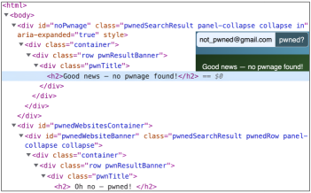
Figure 1. DOM when no pwnage detected.

Figure 2. DOM when pwnage detected.

⬇

1foreach email in list_of_emails:

2 EnterData( email, //input[@id=’account’] ) # enter each email to search box

3 Click( //button[@id=’searchPwnage’] ) # click search button

4 ScrapeText( //div[@aria-expanded=’true’]//h2 ) # scrape pwnage message

Figure 3. A web automation program that scrapes pwnage result for each email address from a list.

Synthesizing web automation programs. In general, implementing web automation programs requires creating both the desired control-flow structure (with arbitrarily nested loops potentially) and identifying generalizable selectors for all of its instructions; this is very hard and time-consuming. WebRobot (Dong et al., 2022) is a state-of-the-art technique that allows non-experts to create web automation programs from a short trace $A$ of user actions (e.g., clicking a button, scraping text). A key underpinning idea is its trace semantics: given a program $P$, trace semantics outputs a sequence $A^{\prime}$ of actions that $P$ executes, by resolving any free variables (such as the local loop variable from Figure 3). Then, one can check if $P$ satisfies $A$ by checking if $P$’s output trace $A^{\prime}$ matches $A$.

Key challenge: synthesizing programs with local variables. While trace semantics significantly bridges the gap between programming-by-demonstration (PBD) and programming-by-example (PBE) by enabling a “guess-and-check” style synthesis approach for web automation (Dong et al., 2022; Pu et al., 2022; Chen et al., 2023; Pu et al., 2023), state-of-the-art synthesis algorithms unfortunately fail to scale to challenging web automation tasks due to the heavy use of local variables in those tasks. Consider the enormous space of potential loop bodies to be searched. All these bodies use loop variables and therefore must be evaluated under an extended context that also binds such local variables to values. Conventional observational equivalence (OE) from the program synthesis literature (Udupa et al., 2013; Albarghouthi et al., 2013) fundamentally cannot reduce this space: they track bindings for only input variables, but not for local variables. As a result, they cannot build equivalence classes for loop bodies, and hence fall back to enumeration. The only existing work (to our best knowledge) that pushed the boundary of OE is RESL (Peleg et al., 2020). Briefly, its idea is to “infer” bindings for local variables given a higher-order sketch, which enables applying OE over the space of lambda bodies. A fundamental problem, however, is the data dependency across iterations (for functions like fold). Its implication to synthesis is succinctly summarized by RESL as a “chicken-and-egg” problem: we need output values of programs in order to apply OE for more efficient synthesis, but we need the programs first in order to obtain their output values. This cyclic dependency fundamentally limits all prior work (such as RESL, among others (Feser et al., 2015; Smith and Albarghouthi, 2016)) to sketch-based approaches with crafted binding-inference rules, which still resort to enumeration in many cases. The general problem of how to reduce the space of programs with local variables remains open (Peleg et al., 2020).

Our idea: lifted interpretation. The same problem occurs in our domain: as we will show shortly, loops in web automation use local variables and exhibit data dependency across iterations. In this work, we propose a new algorithm that can apply OE-based reduction for any programs, without requiring binding inference. We build upon the OE definition from RESL (Peleg et al., 2020): two programs belong to the same equivalence class if they share the same context and yield the same output. Notably, “context” here is a binding context with all free variables including both input and local variables. Our key insight can be summarized as follows.

We can compute an equivalence relation of programs based on OE under all reachable contexts, by creating equivalence classes simultaneously while evaluating all programs from a given tree grammar (with respect to a given input). Furthermore, we can use (a generalized form of) finite tree automata to compactly store the equivalence relation.

Here, a reachable context is one that emerges during the execution of at least one program from the grammar, for a given input. Furthermore, programs rooted at the same grammar symbol share reachable contexts. For instance, the loop from Figure 3 introduces the same binding context for loop bodies that can be put inside it. However, computing reachable contexts requires program evaluation which again requires reachable contexts — this is the aforementioned “chicken-and-egg” problem described in RESL (Peleg et al., 2020). To break this cycle, our key insight is to simultaneously evaluate all programs top-down from the grammar, during which we construct equivalence classes of programs bottom-up based on their outputs under their reachable contexts. This idea essentially lifts up an interpreter from evaluating one single program at a time to simultaneously evaluating all programs from a grammar, with respect to a given input. This lifted interpretation process allows us to systematically enumerate all reachable contexts, and hence build equivalence classes for all programs including those with local variables.

General idea, instantiation, and evaluation. In the rest of this paper, we first illustrate how our idea works in general in Section 3 using a small functional language. Then, in Section 4, we present an instantiation of our approach in the domain of web automation. We implement this instantiation in a tool called Arborist. Our evaluation results show that Arborist can solve more challenging benchmarks using much less time, significantly advancing the state-of-the-art for web automation.

Contributions. This paper makes the following contributions.

• We propose a new synthesis algorithm, based on lifted interpretation and finite tree automata, that can reduce the search space of programs with local variables.

• We instantiate this approach in the domain of web automation and develop a new programming-by-demonstration algorithm.

• We implement our technique in a tool called Arborist and evaluate it on 131 benchmarks. Our results highlight that the idea of lifted interpretation yields a significantly faster synthesizer.

2. Preliminaries

In this section, we review the standard concepts of observational equivalence (OE) and finite tree automata (FTAs) from the literature, focusing on their application to program synthesis.

2.1. Synthesis using Observational Equivalence

Observational equivalence (OE) was originally proposed by Hennessy and Milner (1980) to define the semantics of concurrent programs, and has been used widely within the programming languages community. Intuitively, two terms are observationally equivalent whenever they are interchangeable in all observable contexts. In the field of programming-by-example (PBE), OE has been utilized to reduce the search space of programs, typically in bottom-up synthesis algorithms.

Bottom-up synthesis. Bottom-up algorithms synthesize programs by first constructing smaller programs which are later used as building blocks to create bigger ones. Specifically, the algorithm begins with an initial set $W$ containing all atomic programs of size 1 (e.g., input variables, constants), and then iteratively grows $W$ by adding new programs of larger sizes that are composed of those already in $W$. The algorithm terminates when $W$ has a program $P$ that meets the given specification. For instance, for a language that includes variable $x$ and integer constants $1$ and $2$, $W$ is initially $\{x,1,2\}$ but later will contain more terms such as $x+1$ and $x+2$, assuming $+$ operator is allowed by the language. If the specification is given as an input-output example pair $(1,3)$ meaning “return $3$ when $x=1$”, then $x+2$ is a correct program whereas $x+1$ is not.

Observational equivalence reduction. Bottom-up synthesis often uses observational equivalence to reduce the program space in order to improve the search efficiency. The key idea is to not add a new program $P$ to $W$, if there already exists some $P^{\prime}\in W$ that behaves the same as $P$ observationally. In particular, existing PBE work (Albarghouthi et al., 2013; Udupa et al., 2013) defines two programs $P_{1},P_{2}$ to be observationally equivalent if they yield the same output on each input example. This idea keeps only programs that are observationally distinct (given input examples), thereby reducing the size of $W$ and accelerating the search. RESL (Peleg et al., 2020) further generalizes OE to consider an extended context that also includes local variables: two programs are observationally equivalent if they yield the same output given a shared context (which may include local variables). However, conventional bottom-up synthesis algorithms no longer work under this OE definition, as they cannot evaluate programs with free local variables before knowing their binding context.

2.2. Synthesis using Finite Tree Automata

OE essentially defines an equivalence relation of programs, which can be stored using finite tree automata (FTAs) (Wang et al., 2017a).

Finite tree automata. Finite tree automata (FTAs) (Comon et al., 2008) deal with tree-structured data: they generalize standard finite (word) automata by accepting trees rather than words/strings.

Definition 2.1 (Finite Tree Automata).

A (bottom-up) finite tree automaton (FTA) over alphabet $F$ is a tuple $\mathcal{A}=(Q,F,Q_{f},\Delta)$, where $Q$ is a set of states, $Q_{f}\subseteq Q$ is a set of final states, and $\Delta$ is a set of transitions of the form $f(q_{1},\cdots,q_{n})\rightarrow q$ where $q_{1},\cdots,q_{n},q\in Q$ and $f\in F$. A term $t$ is accepted by $\mathcal{A}$ if $t$ can be rewritten to a final state according to the transitions (i.e., rewrite rules). The language of $\mathcal{A}$, denoted $L(\mathcal{A})$, is the set of terms accepted by $\mathcal{A}$.

Notations. We also use $\mathcal{A}=(Q_{f},\Delta)$ as a simpler notation, since $Q$ and $F$ can be determined by $\Delta$. We use $\textit{SubFTA}(q,\mathcal{A})$ to mean the sub-FTA of $\mathcal{A}$ that is rooted at state $q$.

Program synthesis using FTAs. Given a tree grammar $G$ defining the syntax of a language and given an input-output example $\mathcal{E}=(\mathcal{E}_{\emph{in}},\mathcal{E}_{\emph{out}})$, we can construct an FTA $\mathcal{A}=(Q,F,Q_{f},\Delta)$, such that $L(\mathcal{A})$ contains all programs from $G$ (up to a finite size) that satisfy $\mathcal{E}$. In particular, the alphabet $F$ consists of all operators from $G$. We have a state $q^{c}_{s}\in Q$ if there exists a program rooted at symbol $s$ from $G$ that outputs $c$ given input $\mathcal{E}_{\emph{in}}$. We have a transition $f(q^{c_{1}}_{s_{1}},\cdots,q^{c_{n}}_{s_{n}})\rightarrow q^{c_{0}}_{s_{0}}\in\Delta$ if applying function $f$ on $c_{1},\cdots,c_{n}$ yields $c_{0}$. A state $q^{c}_{s}$ is marked final if $c=\mathcal{E}_{\emph{out}}$ and $s$ is a start symbol of $G$. Once $\mathcal{A}$ is constructed, one can extract a program $P$ from $L(\mathcal{A})$ heuristically (e.g., smallest in size) and return $P$ as the final synthesized program (Wang et al., 2017a).

Remarks. Every state $q^{c}_{s}\in Q$ represents an equivalence class of all programs rooted at grammar symbol $s$ that produce the same value $c$ on $\mathcal{E}_{\emph{in}}$. In other words, $q^{c}_{s}$ stores all observationally equivalent programs. To our best knowledge, all existing FTA-based synthesis techniques (Wang et al., 2017a, b, 2018b; Yaghmazadeh et al., 2018; Miltner et al., 2022) are based on the notion of OE that considers only input variables. In other words, all existing techniques resort to enumeration of programs with free local variables (Peleg et al., 2020).

3. Lifted Interpretation

This section illustrates how the general idea of lifted interpretation works on a simple functional language. Section 4 will later describe a full-fledged instantiation to the domain of web automation.

3.1. A Simple Programming-by-Example Task

Example 3.1.

Given the simple functional language from Figure 4, let us consider the following programming-by-example (PBE) task: synthesize a program that returns $7$ given input list $[1,2,4]$. Suppose the intended program is:

$$P_{1}:\textnormal{fold}\big{(}x,(acc,elem)\Rightarrow\textnormal{add}(acc,elem)\big{)}$$

which calculates the sum of all elements from the input list $x$. Consider another program:

$$P_{2}:\textnormal{fold}\big{(}x,(acc,elem)\Rightarrow\textnormal{add}(\textnormal{mult}(acc,2),1)\big{)}$$

which returns the same output $7$ as $P_{1}$, given the example input $[1,2,4]$. Notably, while the lambda bodies in $P_{1}$ and $P_{2}$ are different, they share the same context-output behaviors (or footprint), for the given input list. Please see Table 1 which shows their local variable bindings and corresponding output values across all iterations. In what follows, we will illustrate how to synthesize $P_{1}$ and $P_{2}$ from the input-output example $[1,2,4]\mapsto 7$, using our lifted interpretation idea.

$$\begin{array}[]{rll}P&::=&\textnormal{fold}\big{(}L,(acc,elem)\Rightarrow E\big{)}\\ E&::=&acc\ |\ elem\ |\ 1\ |\ 2\ |\ \textnormal{add}(E,E)\ |\ \textnormal{mult}(E,E)\\ L&::=&x\\ \end{array}$$

Figure 4. A simple functional language. Here, $x$ is the input variable, which is a list of integers. We simplify the standard fold operator to use a default seed of $0$ (which is implicit and not shown as an argument). Note that fold introduces two local variables: $acc$ is the accumulator, and $elem$ will be bound to each element from $L$. $E$ is the lambda body, which may use local variables $acc$ and $elem$. The “add” and “mult” operators are the standard addition and multiplication.

Table 1. Footprints of lambda bodies from $P_{1}$ and $P_{2}$ respectively, across all iterations.

	local variable bindings	$P_{1}$: $\textnormal{add}(acc,elem)$	$P_{2}$: $\textnormal{add}(\textnormal{mult}(acc,2),1)$
iteration 1	$acc\mapsto 0,\ \ elem\mapsto 1$	1	1
iteration 2	$acc\mapsto 1,\ \ elem\mapsto 2$	3	3
iteration 3	$acc\mapsto 3,\ \ elem\mapsto 4$	7	7

3.2. FTAs based on Observational Equivalence

Let us first present a new FTA-based data structure that our lifted interpretation approach utilizes to succinctly encode equivalence classes of programs. The main ingredient is its generalization of the FTA state definition from prior work (Wang et al., 2017a): our state includes a context $C$ which contains information (e.g., all variable bindings) to evaluate programs with free local variables. In particular, we define an FTA state $q$ as a pair:

$$(\textsf{s},\Omega)\ \ \emph{where}\ \ \Omega=\{\ C_{1}\mapsto O_{1},\cdots,C_{l}\mapsto O_{l}\ \}$$

Here, s is a grammar symbol, and $\Omega$ is a footprint which maps a context $C_{i}$ to an output $O_{i}$. Each entry $C_{i}\mapsto O_{i}$ is called a behavior; so a footprint is a set of behaviors. Intuitively, if there exists a program $P$ rooted at s that evaluates to $O_{i}$ under $C_{i}$ for all $i\in[1,l]$, then our FTA $\mathcal{A}$ has a state $(\textsf{s},\{C_{1}\mapsto O_{1},\cdots,C_{l}\mapsto O_{l}\})$, and vice versa. A context is reachable if it can actually emerge, when executing programs in a given grammar for a given input. Given a finite grammar, if all programs terminate, then the number of reachable contexts is finite. Our work assumes a finite number of reachable contexts, which we believe is a reasonable assumption for program synthesis.

The remaining definitions are relatively standard. Our alphabet $F$ includes all operators from the programming language. A transition $\delta\in\Delta$ is of the form $f(q_{1},\cdots,q_{n})\rightarrow q$ which connects multiple states to one state. However, because our state definition is more general, the condition under which to include a transition now becomes different from prior work (Wang et al., 2017a). Specifically, $\mathcal{A}$ includes a transition $\delta=f(q_{1},\cdots,q_{n})\rightarrow q$, if for every behavior $C\mapsto O$ in $q$, we have behavior $C_{k}\mapsto O_{k}$ in $q_{k}$ (for all $k\in[1,n]$), such that according to $f$’s semantics and given $C_{1}\mapsto O_{1},\cdots,C_{n}\mapsto O_{n}$, evaluating $f$ under context $C$ indeed yields output $O$.

3.3. Illustrating Lifted Interpretation

Now we are ready to explain how our lifted interpretation idea works for Example 3.1.

Setup. First, we build an FTA $\mathcal{A}_{s}=(\{q_{1}\},\Delta_{s})$ — see Figure 7 — for the grammar in Figure 4. We will later apply lifted interpretation to $\mathcal{A}_{s}$. Each state in $\mathcal{A}_{s}$ is annotated with a grammar symbol and an empty footprint. Notice the cyclic transitions around $q_{3}$, due to the recursive add and mult productions. This induces an infinite space of programs — our approach finitizes the grammar by bounding the size of its programs, as standard in the literature (Wang et al., 2017a).

Applying lifted interpretation. Then, we use lifted interpretation to “evaluate” $\mathcal{A}_{s}$ under an initial context, which would eventually produce another FTA $\mathcal{A}_{e}=(\{q_{11}\},\Delta_{e})$ (see a part of it in Figure 7). Different from $\mathcal{A}_{s}$, $\mathcal{A}_{e}$ will cluster programs (including all sub-programs) into equivalence classes based on OE. Figure 7 shows the annotations (i.e., grammar symbols and footprints) for $\mathcal{A}_{e}$.

At a high-level, lifted interpretation traverses $\mathcal{A}_{s}$ systematically, computes reachable contexts on-the-fly during traversal, and most importantly, constructs the equivalence classes simultaneously given these reachable contexts. In particular, given an initial context $C$ and an FTA $\mathcal{A}_{s}=(Q_{f},\Delta)$ with final states $Q_{f}$ and transitions $\Delta$, lifted interpretation returns an FTA $\mathcal{A}_{e}=(Q^{\prime}_{f},\Delta^{\prime})$ with final states $Q^{\prime}_{f}$ and transitions $\Delta^{\prime}$, such that if two programs from $L(\mathcal{A}_{s})$ yield the same output under $C$, then they belong to the same (final) state in $\mathcal{A}_{e}$. More specifically, we have:

$$\begin{array}[]{rcc}Q^{\prime}_{f}&=&\big{\{}\ q^{\prime}_{i}\ \ \big{|}\ \ q_{i}\in Q_{f},\ \ C\vdash q_{i};\Delta\rightsquigarrow(q^{\prime}_{i},\Delta^{\prime}_{i})\ \big{\}}\\[5.0pt] \Delta^{\prime}&=&\bigcup_{q_{i}\in Q_{f}}{\Delta^{\prime}_{i}}\ \ \ \textnormal{ where }C\vdash q_{i};\Delta\rightsquigarrow(q^{\prime}_{i},\Delta^{\prime}_{i})\end{array}$$

That is, if any final state $q_{i}$ in $\mathcal{A}_{s}$ “evaluates to” a state $q^{\prime}_{i}$ under $C$, then $q^{\prime}_{i}$ is a final state of $\mathcal{A}_{e}$. This process also yields a set $\Delta^{\prime}_{i}$ of transitions for each $q_{i}$, which are added as transitions to $\mathcal{A}_{e}$.

Key judgment. The key judgment that drives the lifted interpretation process is of the following form. Note that this judgment is non-deterministic; that is, a state may evaluate to multiple states.

$$\begin{array}[]{c}C\vdash q;\Delta\rightsquigarrow(q^{\prime},\Delta^{\prime})\end{array}$$

It reads as follows: given context $C$, state $q$ (with respect to transitions $\Delta$) evaluates to state $q^{\prime}$ with transitions $\Delta^{\prime}$. The guarantee is that: for all programs $P$ from $L(\{q\},\Delta)$ that yield the same output under context $C$, we have one unique state $q^{\prime}$ (and transitions $\Delta^{\prime}$) such that these programs $P$ are in $L(\{q^{\prime}\},\Delta^{\prime})$. For instance, given $C=\{x\mapsto[1,2,4]\}$, $q_{1}$ from $\mathcal{A}_{s}$ may evaluate to $q_{11}$ in $\mathcal{A}_{e}$: all programs in $L(\{q_{1}\},\Delta_{s})$ that yield $7$ given $C$ are merged into state $q_{11}$.

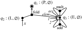
Figure 5. FTA $\mathcal{A}_{s}$ constructed for grammar from Figure 4. Each FTA state is annotated with a grammar symbol and a footprint (which maps a reachable context to a value).

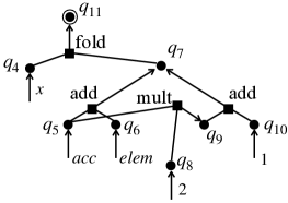
Figure 6. A part of $\mathcal{A}_{e}$ after applying lifted interpretation on $\mathcal{A}_{s}$ from Figure 7. Annotations on FTA states can be found in Figure 7.

$$\begin{array}[]{ll}q_{4}:\big{(}\ \ \textsf{L},\left\{\begin{array}[]{l}\{x\mapsto[1,2,4]\}\mapsto[1,2,4]\end{array}\right\}\ \ \big{)}\par\\ \\ q_{5}:(\textsf{E},\left\{\begin{array}[]{l}\left\{\begin{array}[]{l}x\mapsto[1,2,4]\\ acc\mapsto 0\\ elem\mapsto 1\end{array}\right\}\mapsto 0\\[15.0pt] \left\{\begin{array}[]{l}x\mapsto[1,2,4]\\ acc\mapsto 1\\ elem\mapsto 2\end{array}\right\}\mapsto 1\\[15.0pt] \left\{\begin{array}[]{l}x\mapsto[1,2,4]\\ acc\mapsto 3\\ elem\mapsto 4\end{array}\right\}\mapsto 3\end{array}\right\})\ \ q_{6}:(\textsf{E},\left\{\begin{array}[]{l}\left\{\begin{array}[]{l}x\mapsto[1,2,4]\\ acc\mapsto 0\\ elem\mapsto 1\end{array}\right\}\mapsto 1\\[15.0pt] \left\{\begin{array}[]{l}x\mapsto[1,2,4]\\ acc\mapsto 1\\ elem\mapsto 2\end{array}\right\}\mapsto 2\\[15.0pt] \left\{\begin{array}[]{l}x\mapsto[1,2,4]\\ acc\mapsto 3\\ elem\mapsto 4\end{array}\right\}\mapsto 4\end{array}\right\})\ \ q_{7}:(\textsf{E},\left\{\begin{array}[]{l}\left\{\begin{array}[]{l}x\mapsto[1,2,4]\\ acc\mapsto 0\\ elem\mapsto 1\end{array}\right\}\mapsto 1\\[15.0pt] \left\{\begin{array}[]{l}x\mapsto[1,2,4]\\ acc\mapsto 1\\ elem\mapsto 2\end{array}\right\}\mapsto 3\\[15.0pt] \left\{\begin{array}[]{l}x\mapsto[1,2,4]\\ acc\mapsto 3\\ elem\mapsto 4\end{array}\right\}\mapsto 7\end{array}\right\})\par\\ \\ q_{8}:(\textsf{E},\left\{\begin{array}[]{l}\left\{\begin{array}[]{l}x\mapsto[1,2,4]\\ acc\mapsto 0\\ elem\mapsto 1\end{array}\right\}\mapsto 2\\[15.0pt] \left\{\begin{array}[]{l}x\mapsto[1,2,4]\\ acc\mapsto 1\\ elem\mapsto 2\end{array}\right\}\mapsto 2\\[15.0pt] \left\{\begin{array}[]{l}x\mapsto[1,2,4]\\ acc\mapsto 3\\ elem\mapsto 4\end{array}\right\}\mapsto 2\end{array}\right\})\ \ q_{9}:(\textsf{E},\left\{\begin{array}[]{l}\left\{\begin{array}[]{l}x\mapsto[1,2,4]\\ acc\mapsto 0\\ elem\mapsto 1\end{array}\right\}\mapsto 0\\[15.0pt] \left\{\begin{array}[]{l}x\mapsto[1,2,4]\\ acc\mapsto 1\\ elem\mapsto 2\end{array}\right\}\mapsto 2\\[15.0pt] \left\{\begin{array}[]{l}x\mapsto[1,2,4]\\ acc\mapsto 3\\ elem\mapsto 4\end{array}\right\}\mapsto 6\end{array}\right\})\ \ q_{10}:(\textsf{E},\left\{\begin{array}[]{l}\left\{\begin{array}[]{l}x\mapsto[1,2,4]\\ acc\mapsto 0\\ elem\mapsto 1\end{array}\right\}\mapsto 1\\[15.0pt] \left\{\begin{array}[]{l}x\mapsto[1,2,4]\\ acc\mapsto 1\\ elem\mapsto 2\end{array}\right\}\mapsto 1\\[15.0pt] \left\{\begin{array}[]{l}x\mapsto[1,2,4]\\ acc\mapsto 3\\ elem\mapsto 4\end{array}\right\}\mapsto 1\end{array}\right\})\par\\ \\ q_{11}:\big{(}\ \ \textsf{P},\left\{\begin{array}[]{l}\{x\mapsto[1,2,4]\}\mapsto 7\end{array}\right\}\ \ \big{)}\par\par\end{array}$$

Figure 7. Annotations (i.e., grammar symbols and footprints) for all states in $\mathcal{A}_{e}$ from Figure 7.

Inference rules. The key inference rule that implements this judgment is the Transition rule:

$$\small\centering\begin{array}[]{c}\textsc{(Transition)}\ \ \mkern-2.0mu\displaystyle\frac{\begin{array}[]{c}\delta=f(q_{1},\cdots,q_{n})\rightarrow q\in\Delta\ \ \ \ \ \ C\vdash\delta;\Delta\rightsquigarrow(q^{\prime},\Delta^{\prime})\end{array}}{\vphantom{,}C\vdash q;\Delta\rightsquigarrow(q^{\prime},\Delta^{\prime})}\mkern-2.0mu\end{array}\@add@centering$$

It says: evaluating a state $q$ boils down to evaluating each of $q$’s incoming transitions $\delta$. For instance, to evaluate $q_{1}$ in $\mathcal{A}_{s}$ (see Figure 7) under $C=\{x\mapsto[1,2,4]\}$, we would evaluate $\textnormal{fold}(q_{2},q_{3})\rightarrow q_{1}$ under $C$. The following inference rules describe how to actually evaluate a fold transition.

$$\small\centering\begin{array}[]{lc}\textsc{(Fold-1)}&\mkern-2.0mu\displaystyle\frac{\begin{array}[]{c}C\vdash q_{1};\Delta\rightsquigarrow(q^{\prime}_{1},\Delta^{\prime}_{1})\ \ \ \ C\mapsto lst\in\textit{Footprint}(q^{\prime}_{1})\ \ \ \ C,lst\vdash q_{2};\Delta\rightsquigarrow(q^{\prime}_{2},\Delta^{\prime}_{2})\\ v_{0}=0\ \ \ \ C\big{[}acc\mapsto v_{i-1},elem\mapsto lst[i]\big{]}\mapsto v_{i}\in\textit{Footprint}(q^{\prime}_{2})\ \ \ \ i\in[1,|lst|]\\ \Omega=\textit{Footprint}(q)\ \ \ \ \Omega^{\prime}=\Omega\cup\{C\mapsto v_{|lst|}\}\ \ \ \ q^{\prime}=\textit{MkState}(\textsf{P},\Omega^{\prime})\end{array}}{\vphantom{,}C\vdash\textnormal{fold}(q_{1},q_{2})\rightarrow q;\Delta\rightsquigarrow(q^{\prime},\Delta^{\prime}_{1}\cup\Delta^{\prime}_{2}\cup\{\textnormal{fold}(q^{\prime}_{1},q^{\prime}_{2})\rightarrow q^{\prime}\})}\mkern-2.0mu\\ \\ \textsc{(Fold-2)}&\mkern-2.0mu\displaystyle\frac{\begin{array}[]{c}v_{0}=0\ \ \ \ q^{\prime}_{0}=q\ \ \ \ \Delta^{\prime}_{0}=\Delta\ \ \ \ i\in[1,|lst|]\ \ \ \ C_{i-1}=C\big{[}acc\mapsto v_{i-1},elem\mapsto lst[i]\big{]}\\ C_{i-1}\vdash q^{\prime}_{i-1};\Delta^{\prime}_{i-1}\rightsquigarrow(q^{\prime}_{i},\Delta^{\prime}_{i})\ \ \ \ C_{i-1}\mapsto v_{i}\in\textit{Footprint}(q^{\prime}_{i})\end{array}}{\vphantom{,}C,lst\vdash q;\Delta\rightsquigarrow(q^{\prime}_{|lst|},\Delta^{\prime}_{|lst|})}\mkern-2.0mu\end{array}\@add@centering$$

Let us take $\textnormal{fold}(q_{2},q_{3})\rightarrow q_{1}$ from $\mathcal{A}_{s}$ as an example and explain how these two rules work.

The Fold-1 rule first evaluates $q_{2}$ from $\mathcal{A}_{s}$ to $q_{4}$ in $\mathcal{A}_{e}$, which, as mentioned above, boils down to evaluating $q_{2}$’s incoming transition $x\rightarrow q_{2}$. This is done using the following Input-Var rule.

$$\small\centering\begin{array}[]{lc}\textsc{(Input-Var)}&\mkern-2.0mu\displaystyle\frac{\begin{array}[]{c}C[x]=lst\ \ \ \ \Omega=\textit{Footprint}(q)\ \ \ \ \Omega^{\prime}=\Omega\cup\{C\mapsto lst\}\ \ \ \ q^{\prime}=\textit{MkState}(\textsf{L},\Omega^{\prime})\end{array}}{\vphantom{,}C\vdash x\rightarrow q;\Delta\rightsquigarrow(q^{\prime},\{x\rightarrow q^{\prime}\})}\mkern-2.0mu\end{array}\@add@centering$$

Specifically, Input-Var first obtains the value $lst$, which is $[1,2,4]$, that $x$ binds to. Then it creates a footprint $\Omega^{\prime}$ that includes all behaviors from $q$ and a new binding $C\mapsto lst$. Finally, a new state $q^{\prime}$ is created, with grammar symbol L and footprint $\Omega^{\prime}$. Here, MkState is simply a state constructor. In our example, Input-Var yields $q_{4}$, which has footprint $\{\{x\mapsto[1,2,4]\}\mapsto[1,2,4]\}$: it means all programs in $L(\{q_{4}\},\Delta_{e})$ produce $[1,2,4]$ given context $C=\{x\mapsto[1,2,4]\}$.

Popping up to Fold-1, given $q_{4}$, it retrieves the output $lst$ for $q_{4}$ given context $C$, notably, by looking up $q_{4}$’s footprint. It then uses an auxiliary rule, Fold-2, to evaluate $q_{3}$ from $\mathcal{A}_{s}$ — which corresponds to lambda bodies — given $C$ and $lst$. This yields $q_{7}$ in $\mathcal{A}_{e}$, among potentially other states which are not shown in Figure 7. Again, the guarantee is: all programs in $L(\{q_{7}\},\Delta_{e})$ share the same footprint. Now given $q_{7}$, Fold-1 finally creates $q_{11}$ in $\mathcal{A}_{e}$, as well as transition $\textnormal{fold}(q_{4},q_{7})\rightarrow q_{11}$. The key is to compute $q_{11}$’s footprint $\Omega^{\prime}$, which inherits everything from $q_{1}$’s footprint $\Omega$ but also includes additionally the behavior $C\mapsto v_{|lst|}$. Here, $v_{|lst|}$ (which is $v_{3}$ in our example, as $|lst|=3$) is the output for the fold operation, under context $C=\{x\mapsto[1,2,4]\}$ which is the input example we are concerned with. We note that the computation of $v_{|lst|}$ is based on looking up $q_{7}$’s footprint.

Now let us briefly explain how the Fold-2 rule evaluates $q_{3}$ to $q_{7}$. The evaluation is an iterative process that follows the fold semantics. It begins with context $C_{0}$ that binds the accumulator $acc$ to the default seed $0$ and binds $elem$ to the first element of $lst$, then recursively evaluates $q^{\prime}_{0}$ (i.e., $q_{3}$ in our example) under $C_{0}$ which yields $q^{\prime}_{1}$ (not shown in Figure 7), and finally obtains $v_{1}$ (which $acc$ should be bound to in the next iteration) by (again) looking up the footprint of $q^{\prime}_{1}$. Note that $q^{\prime}_{1}$ is an intermediate state whose footprint has one behavior, since we have only seen $C_{0}$ so far. The second iteration will repeat the same process but for $q^{\prime}_{1}$ and using $C_{1}$, which would yield $q^{\prime}_{2}$ whose footprint has two behaviors. This process continues until we reach the end of $lst$, eventually yielding $q^{\prime}_{|lst|}$; $q_{7}$ in $\mathcal{A}_{e}$ is one such state. As shown in Figure 7, $q_{7}$ has three behaviors in its footprint.

We skip the discussion of the other rules which are used to construct all the other states in $\mathcal{A}_{e}$, and refer readers to the appendix of our paper for a complete list of rules. In the end, given $\mathcal{A}_{e}$, we will mark states whose footprint satisfies the specification as final states, and extract a program from $\mathcal{A}_{e}$. In our example, $q_{11}$ is final, and both $P_{1}$ and $P_{2}$ are in $L(\{q_{11}\},\Delta_{e})$.

4. Instantiation to Web Automation

This section presents a full-fledged instantiation of the lifted interpretation idea to web automation.

4.1. Web Automation Language

Figure 8 presents our web automation language. The syntax is slightly different from the one in WebRobot (Dong et al., 2022). First, our syntax looks more “functional”: for example, loop bodies are presented as lambdas. This is solely for the purpose of making it easier to later present our approach. Second, the language is also slightly more expressive: ForSelectors allows starting from the $i$-th child/descendant with $i\geq 1$, whereas WebRobot’s syntax requires $i=1$. This extension is motivated by our observation when curating new benchmarks: many tasks require this more relaxed form of loop. We refer interested readers to the WebRobot work for more details about the syntax, but in brief, a web automation program $P$ is always a sequence of statements. It supports different types of statements. For example, Click clicks a DOM element located by selector expression $se$. We use an XPath-like syntax for selector expressions: $se/\psi[i]$ gives the $i$-th child of $se$ that satisfies $\psi$, whereas $\mkern 0.0mu/\mkern-5.0mu/\mkern 0.0mu$ considers $se$’s descendants. $x$ is an input variable that is bound to a user-provided data source (like the list of emails from Example 1), whereas $y$ and $z$ are local variables introduced by and internal to the program. ForData is a loopy statement that iterates over a list of data entries (such as emails from Example 1) given by $de$, binds $z$ to each of them, and executes loop body $P$. ForSelectors is quite similar, but it loops over a list of selector expressions returned by $se$. While handles pagination, where it repeatedly clicks the “next page” button located by $se$ and executes loop body $P$, until $se$ no longer exists on the webpage.

$$\begin{array}[]{rlll}\emph{Program}&P&::=&\emph{Seq}(E,P)\ |\ \emph{skip}\\ \emph{Statement}&E&::=&\emph{Click}(se)\\ &&\ \ \ |&\emph{ScrapeText}(se)\\ &&\ \ \ |&\emph{ScrapeLink}(se)\\ &&\ \ \ |&\emph{Download}(se)\\ &&\ \ \ |&\emph{GoBack}\ |\ \emph{ExtractURL}\\ &&\ \ \ |&\emph{SendKeys}(str,se)\\ &&\ \ \ |&\emph{EnterData}(de,se)\\ &&\ \ \ |&\emph{ForData}(de,\lambda z.P)\\ &&\ \ \ |&\emph{ForSelectors}(se/\psi[i],\lambda y.P)\\ &&\ \ \ |&\emph{ForSelectors}(se\mkern 0.0mu/\mkern-5.0mu/\mkern 0.0mu\psi[i],\lambda y.P)\\ &&\ \ \ |&\emph{While}(\emph{true},P,se)\\ \emph{Selector Expr}&se&::=&\epsilon\ |\ y\ |\ se/\psi[i]\ |\ se\mkern 0.0mu/\mkern-5.0mu/\mkern 0.0mu\psi[i]\\ \emph{Data Expr}&de&::=&x\ |\ z\ |\ de[\emph{key}]\ |\ de[i]\\ \emph{Predicate}&\psi&::=&t\ |\ t[@\tau=str]\\ \end{array}$$

$$\small\begin{array}[]{lc}(\textsc{Seq})&\mkern-2.0mu\displaystyle\frac{\begin{array}[]{c}\Pi,\Gamma\vdash E:A^{\prime}_{1},\Pi^{\prime}_{1}\ \ \ \Pi^{\prime}_{1},\Gamma\vdash P:A^{\prime}_{2},\Pi^{\prime}\\ \end{array}}{\vphantom{,}\Pi,\Gamma\vdash\emph{Seq}(E,P):A^{\prime}_{1}\mkern 0.0mu\texttt{+}\mkern-1.0mu\texttt{+}\mkern 1.0muA^{\prime}_{2},\Pi^{\prime}}\mkern-2.0mu\\ \\ (\textsc{Click})&\mkern-2.0mu\displaystyle\frac{\begin{array}[]{c}\Pi=[\pi_{1},\cdots,\pi_{m}]\ \ \ \pi_{1},\Gamma\vdash se:{\raisebox{1.0pt}{$\chi$}}\\ \Pi^{\prime}=[\pi_{2},\cdots,\pi_{m}]\end{array}}{\vphantom{,}\Pi,\Gamma\vdash\emph{Click}(se):[\emph{Click}({\raisebox{1.0pt}{$\chi$}})],\Pi^{\prime}}\mkern-2.0mu\\ \\ (\textsc{ForData-1})&\mkern-2.0mu\displaystyle\frac{\begin{array}[]{c}\Gamma\vdash de:lst\\ \Pi,\Gamma,lst\vdash P:A^{\prime},\Pi^{\prime}\\ \end{array}}{\vphantom{,}\Pi,\Gamma\vdash\emph{ForData}(de,\lambda z.P):A^{\prime},\Pi^{\prime}}\mkern-2.0mu\\ \\ (\textsc{ForData-2})&\mkern-2.0mu\displaystyle\frac{\begin{array}[]{c}\Pi^{\prime}_{0}=\Pi\ \ \ i\in[1,|lst|]\\ \Pi^{\prime}_{i-1},\Gamma\big{[}z\mapsto lst[i]\big{]}\vdash P:A^{\prime}_{i},\Pi^{\prime}_{i}\\ A^{\prime}=A^{\prime}_{1}\mkern 0.0mu\texttt{+}\mkern-1.0mu\texttt{+}\mkern 1.0mu\cdots\mkern 0.0mu\texttt{+}\mkern-1.0mu\texttt{+}\mkern 1.0muA^{\prime}_{|lst|}\end{array}}{\vphantom{,}\Pi,\Gamma,lst\vdash\emph{ForData}(de,\lambda z.P):A^{\prime},\Pi^{\prime}_{|lst|}}\mkern-2.0mu\end{array}$$

Figure 8. Web automation language. Left is syntax, where $str$ is a string, $i$ is an integer, $t$ is an HTML tag, and $\tau$ is an HTML attribute. Right is a subset of the trace semantics rules; please find the complete set of rules in the appendix.

Figure 8 also presents a subset of the trace semantics rules, which are cleaner than WebRobot’s. The evaluation judgment is of the form:

$$\Pi,\Gamma\vdash P:A^{\prime},\Pi^{\prime}$$

which reads: given a context — consisting of a DOM trace $\Pi$ and a binding environment $\Gamma$ (that binds all free variables in scope) — evaluating program $P$ yields an action trace $A^{\prime}$ and a DOM trace $\Pi^{\prime}$. This evaluation does not execute $P$ in browser; instead, it simulates the execution by “replaying” $P$ given $\Pi$. We refer interested readers to the WebRobot paper (Dong et al., 2022) for the design rationale. Here, we briefly explain a few representative rules. The Seq rule is standard: it evaluates $E$ and $P$ in sequence, and concatenates the resulting action traces. The Click rule is more interesting. It first evaluates $se$ (which may use a variable) under $\pi_{1}$ and $\Gamma$, yielding a selector $\chi$ which is used to form the output action. Then, it removes the first DOM from $\Pi$ to obtain the resulting DOM trace $\Pi^{\prime}$. In other words, the program under evaluation and the DOM trace are always “in sync”: the first action to be executed always corresponds to the first DOM. The ForData rules are perhaps the most interesting. ForData-1 first evaluates $de$ to a list $lst$, and then invokes ForData-2 which is a helper rule that executes all iterations of the loop until termination. The key observation is: similar to the fold function from Example 3.1, ForData also performs dependent iterations; that is, an iteration has to be executed under a context computed by its previous iteration. In particular, the input DOM trace carries the dependency. This data-dependent feature actually is not specific to ForData: all loops in our language are data-dependent, and in fact, Seq is too. Prior work cannot reduce the space of our web automation programs. Our lifted interpretation idea is able to reduce this space, and we will present how it works next.

4.2. Top-Level Synthesis Algorithm

Algorithm 1 shows the top-level algorithm that synthesizes web automation programs from demonstrations. It shares the same interface as WebRobot’s algorithm and thus can be directly integrated with WebRobot’s front-end UI. At a high-level, it takes as input an action trace $A$, a DOM trace $\Pi$, and input data $I$. It returns a program $P$ that generalizes $A$ — i.e., given $\Pi$ and $\Gamma=\{x\mapsto I\}$, evaluating $P$ using trace semantics produces $A^{\prime}$ such that $A$ is a strict prefix of $A^{\prime}$. This generalization is possible, because we require $\Pi$ to have one more DOM than the number of actions in $A$. To synthesize $P$, we first find all programs that reproduce $A$ (i.e., $A^{\prime}$ has $A$ as a prefix) — notably, this process compresses a large number of programs in an FTA $\mathcal{A}$. Then line 12 picks a smallest program $P$, from $\mathcal{A}$, that generalizes $A$. If no such $P$ exists in $\mathcal{A}$, the algorithm returns null.

1: procedure Synthesize($A,\Pi,I$)

2: input: Action trace $A=[a_{1},\cdots,a_{m}]$, DOM trace $\Pi=[\pi_{1},\cdots,\pi_{m},\pi_{m+1}]$, and input data $I$.

3: output: Program $P$ that generalizes $A$, or null if no such program can be found.

4:$\mathcal{A}:=\textsc{InitFTA}([a_{1},\cdots,a_{m}],[\pi_{1},\cdots,\pi_{m}],I)$ where $\mathcal{A}=(Q,F,Q_{f},\Delta)$;

5:while $\mathcal{A}$_is_not_saturated and not_timeout do

6:   $\Delta^{\prime}:=\Delta$;

7:   for all $\delta_{1},\cdots,\delta_{2l}\in\Delta^{\prime}$ where $\delta_{i}=\emph{Seq}(q^{\prime}_{i},q_{i})\rightarrow q_{i-1},i\in[1,2l]$ do

8:$\triangleright$ Find $2l$ “consecutive” transitions.

9:      $\mathcal{A}_{s}:=\textsc{SpeculateFTA}([\delta_{1},\cdots,\delta_{2l}],\Delta)$;

10:      $\mathcal{A}_{e}:=\textsc{EvaluateFTA}(\mathcal{A}_{s},\textit{GetContexts}(q_{0}))$; $\triangleright$ GetContexts gives all contexts in $q_{0}$’s footprint.

11:      $\mathcal{A}:=\textsc{MergeFTAs}(\mathcal{A},q_{0},\mathcal{A}_{e})$;    

12:return $\textsc{Rank}(\mathcal{A},\Pi,I)$;

Algorithm 1: Top-level synthesis algorithm.

Now let us dive into the algorithm a bit more, though more details will be described in subsequent sections. Line 4 initializes $\mathcal{A}$ based on the input traces, such that $\mathcal{A}$ stores all loop-free programs that are guaranteed to reproduce $A$. The reason that we base our synthesis on the input DOM trace $\Pi$ is because selector expressions are not given a priori; they are known only when $\Pi$ becomes available. The input action trace $A$ is used to further guide synthesis. The following example briefly illustrates what an initial FTA looks like; we defer the more detailed explanation to Section 4.4.

Example 4.1.

Consider the following action trace $A=[a_{1},\cdots,a_{6}]$ for the task from Example 1.

$$\small\begin{array}[]{lll}{\color[rgb]{.5,.5,.5}{\footnotesize\texttt{1}}}&\emph{EnterData}(x[0],/html/.../div[1]/input)&{\color[rgb]{.5,.5,.5}{\textsf{\# enter pwned@gmail.com}}}\\ {\color[rgb]{.5,.5,.5}{\footnotesize\texttt{2}}}&\emph{Click}(/html/body/.../div[1]/span/button)&{\color[rgb]{.5,.5,.5}{\textsf{\# click search button}}}\\ {\color[rgb]{.5,.5,.5}{\footnotesize\texttt{3}}}&\emph{ScrapeText}(/html/body/div[1]/.../div/h2)&{\color[rgb]{.5,.5,.5}{\textsf{\# scrape ``Oh no -- pwned!''}}}\\ {\color[rgb]{.5,.5,.5}{\footnotesize\texttt{4}}}&\emph{EnterData}(x[1],/html/.../div[1]/input)&{\color[rgb]{.5,.5,.5}{\textsf{\# enter not\_pwned@gmail.com}}}\\ {\color[rgb]{.5,.5,.5}{\footnotesize\texttt{5}}}&\emph{Click}(/html/body/.../div[1]/span/button)&{\color[rgb]{.5,.5,.5}{\textsf{\# click search button}}}\\ {\color[rgb]{.5,.5,.5}{\footnotesize\texttt{6}}}&\emph{ScrapeText}(/html/body/div[0]/.../div/h2)&{\color[rgb]{.5,.5,.5}{\textsf{\# scrape ``Good news - no pwnage found''}}}\end{array}$$

In addition, the demonstration also includes a DOM trace $\Pi=[\pi_{1},\cdots,\pi_{7}]$, where $a_{i}$ is performed on DOM $\pi_{i}$. Suppose $I=[\text{``{pwned@gmail.com}''},\text{``{not\_pwned@gmail.com}''}]$ is the list of emails.

Figure 10 shows the abstract syntax tree for $A$, and Figure 10 gives the corresponding initial FTA $\mathcal{A}$. Here, we use ${\raisebox{1.0pt}{$\chi$}}_{i}$ as a shorthand to denote the selector in $a_{i}$. Note that $A$ and $\mathcal{A}$ in both figures are pretty much “isomorphic”, except that each action in $\mathcal{A}$ has multiple selectors as “leaf transitions” (see each dashed circle), whereas each action in $A$ has only one selector. Section 4.4 will present more details around how $\mathcal{A}$ is constructed.

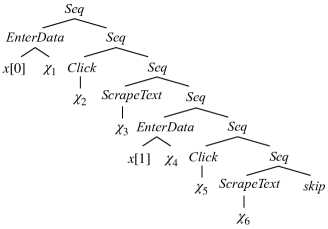
Figure 9. AST for action trace from Example 4.1.

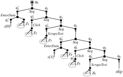
Figure 10. Initial FTA for Figure 10.

Given the initial $\mathcal{A}$, we then enter a loop (lines 5-11) which iteratively adds to $\mathcal{A}$ loopy programs, until no new programs can be found (i.e., $\mathcal{A}$ saturates) or a predefined timeout is reached. In each iteration, we non-deterministically pick $2l$ consecutive Seq transitions $\delta_{1},\cdots,\delta_{2l}$ (line 7), and then perform three key steps: (1) SpeculateFTA guesses an FTA $\mathcal{A}_{s}$ based on these $2l$ transitions, (2) EvaluateFTA performs lifted interpretation over $\mathcal{A}_{s}$, yielding another FTA $\mathcal{A}_{e}$, and (3) MergeFTAs merges $\mathcal{A}_{e}$ into $\mathcal{A}$. The resulting $\mathcal{A}$ at line 11, compared to $\mathcal{A}$ before the merge, includes new loopy programs that are synthesized during this iteration, with the same guarantee that all programs in $\mathcal{A}$ still reproduce $A$. The generalization step takes place in (1), where we reroll a slice of statements in a program from $\mathcal{A}$ to a loop that is then stored in $\mathcal{A}_{s}$. This loop rerolling step, however, is speculative, meaning some rerolled loops may not be correct. Therefore, in step (2), we use EvaluateFTA to check all loops and retain only those that can indeed reproduce $A$ — this EvaluateFTA algorithm (i.e., lifted interpretation) is the key contribution of this paper.

In what follows, we explain how each step works in more detail. In particular, we will begin with EvaluateFTA in Section 4.3, given $\mathcal{A}_{s}$ and its corresponding input contexts. Then in subsequent sections, we explain how FTA initialization, speculation, merging, and ranking work, respectively.

4.3. Lifted Interpretation

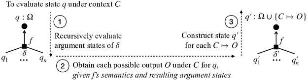
Figure 11. Illustration of EvaluateFTA rules from Figure 12.

As mentioned in Section 3, our lifted interpretation uses the following key judgment.

$$\begin{array}[]{c}C\vdash q;\Delta\rightsquigarrow(q^{\prime},\Delta^{\prime})\end{array}$$

In our domain, a context $C$ consists of a DOM trace $\Pi$ and a binding environment $\Gamma$. Figure 12 shows the EvaluateFTA rules that implement lifted interpretation. We suggest readers looking at Figure 11 at the same time. Rule (1) reduces multi-context evaluation to single-context evaluation. We note that the evaluation under $C_{i}$ relies on the previous evaluation result for $C_{i-1}$. To evaluate a state $q$ under a single context $C$, Rule (2) further reduces it to evaluating each of $q$’s incoming transitions. The remaining rules evaluate various types of transitions; they share the same principle as illustrated in Figure 11. In particular, given transition $\delta=f(q_{1},\cdots,q_{n})\rightarrow q$ and context $C$:

1. First, we recursively evaluate each argument state $q_{i}$. The input context under which to evaluate each $q_{i}$ and the order to evaluate them depends on the semantics of $f$.

2. Given each resulting state $q^{\prime}_{i}$ for $q_{i}$, we obtain the output $O$ for $q$ for $C$. Note that $O$ is computed compositionally, from the corresponding outputs associated with $q^{\prime}_{i}$ and per $f$’s semantics.

3. Finally, we construct state $q^{\prime}$ that $q$ evaluates to. In particular, $q^{\prime}$ includes $C\mapsto O$ as a behavior in its footprint $\Omega$, as well as all behaviors from $q$’s footprint $\Omega$.

Let us examine the rules in detail. Rule (3) is a base case for a nullary transition $\delta$ with no argument states: it directly evaluates the selector expression $se$ and yields a state $q^{\prime}$ with behavior $\Pi,\Gamma\mapsto{\raisebox{1.0pt}{$\chi$}}$. Rule (4) is more interesting. We first evaluate $q_{1}$ to $q^{\prime}_{1}$ under context $\Pi,\Gamma$: note that here we use the context for $q$ to evaluate $q^{\prime}_{1}$, due to Click’s semantics. Then, given $q^{\prime}_{1}$, we obtain its output $\chi$ which is later used to construct the output trace $A^{\prime}$ for $q$. Finally, we construct $q^{\prime}$ with footprint $\Omega^{\prime}$, which includes the new behavior we just created based on $q^{\prime}_{1}$ and Click’s semantics, as well as everything from $\Omega$. Rule (5) considers a Seq transition with two argument states. We first evaluate $q_{1}$ to $q^{\prime}_{1}$. However, before evaluating $q_{2}$, we need to obtain $\Pi^{\prime}_{1}$ from $q^{\prime}_{1}$ to form the context to evaluate $q_{2}$. The output action traces $A^{\prime}_{1},A^{\prime}_{2}$ for $q^{\prime}_{1},q^{\prime}_{2}$ form the output action trace for $q$. Finally, we construct $q^{\prime}$ with $\Omega^{\prime}$, same as previous rules. Rule (6) is another base case for skip. Rule (7) also concerns a base case: if the input DOM trace is empty, it yields the sub-FTA rooted at $q$. Note that in general, $q$ would also include $\texttt{[]},\Gamma\mapsto\texttt{[]},\texttt{[]}$ in its footprint. Rule (7) does not show this explicitly, because we assume all states implicitly have $\texttt{[]},\_\mapsto\texttt{[]},\texttt{[]}$.

Now let us look at the most exciting rules for loops. Consider ForData: its first argument is a data expression that yields a list $lst$, and the second argument (i.e., loop body) is evaluated with the loop variable $z$ being bound to each element from $lst$. To evaluate $q$ with an incoming ForData transition, Rule (8) first evaluates $q_{1}$ to $q^{\prime}_{1}$ and obtains $lst$ from $q^{\prime}_{1}$. Then, we evaluate “loop body” state $q_{2}$ under a context with $lst$: Rule (9) presents how this evaluation works. Intuitively, Rule (9) has a series of $n$ evaluations: $q$ to $q^{\prime}_{1}$, $q^{\prime}_{1}$ to $q^{\prime}_{2}$, $\cdots$, $q^{\prime}_{n-1}$ to $q^{\prime}_{n}$. Note that the output DOM trace for $q^{\prime}_{i}$ is part of the context for evaluating $q^{\prime}_{i+1}$, due to the data dependency across iterations. The output state is $q^{\prime}_{n}$, which encapsulates information from all $n$ iterations. Popping up back to Rule (8): given $q^{\prime}_{2}$, we obtain the output traces $A^{\prime}_{i}$ for all iterations, which are then concatenated to form the output trace in $q^{\prime}$. We skip the discussion on other loop types as they are very similar to ForData.

$\displaystyle\small\centering\begin{array}[]{l}(1)\ \mkern-2.0mu\displaystyle\frac{\begin{array}[]{c}q^{\prime}_{0}=q\ \ \ \Delta^{\prime}_{0}=\Delta\ \ \ \ C_{i}\vdash q^{\prime}_{i-1};\Delta^{\prime}_{i-1}\rightsquigarrow(q^{\prime}_{i},\Delta^{\prime}_{i})\end{array}}{\vphantom{,}C_{1},\cdots,C_{n}\vdash q;\Delta\rightsquigarrow(q^{\prime}_{n},\Delta^{\prime}_{n})}\mkern-2.0mu\par\ \ \par(2)\ \mkern-2.0mu\displaystyle\frac{\begin{array}[]{c}\delta=f(q_{1},\cdots,q_{n})\rightarrow q\in\Delta\ \ \ C\vdash\delta;\Delta\rightsquigarrow(q^{\prime},\Delta^{\prime})\end{array}}{\vphantom{,}C\vdash q;\Delta\rightsquigarrow(q^{\prime},\Delta^{\prime})}\par\mkern-2.0mu\\ \\ (3)\ \mkern-2.0mu\displaystyle\frac{\begin{array}[]{c}\Pi=[\pi_{1},\cdots,\pi_{m}]\ \ \ \ \Gamma,\pi_{1}\vdash se:{\raisebox{1.0pt}{$\chi$}}\ \ \ \ \Omega=\textit{Footprint}(q)\ \ \ \ \Omega^{\prime}=\Omega\cup\{\Pi,\Gamma\mapsto{\raisebox{1.0pt}{$\chi$}}\}\ \ \ \ q^{\prime}=\textit{MkState}(\textsf{se},\Omega^{\prime})\end{array}}{\vphantom{,}\Pi,\Gamma\vdash se\rightarrow q;\Delta\rightsquigarrow(q^{\prime},\{se\rightarrow q^{\prime}\})}\par\mkern-2.0mu\\ \\ (4)\ \mkern-2.0mu\displaystyle\frac{\begin{array}[]{c}\Pi,\Gamma\vdash q_{1};\Delta\rightsquigarrow(q^{\prime}_{1},\Delta^{\prime}_{1})\ \ \ \ \Pi,\Gamma\mapsto{\raisebox{1.0pt}{$\chi$}}\in\textit{Footprint}(q^{\prime}_{1})\ \ \ \ \Omega=\textit{Footprint}(q)\ \ \ \ \Pi=[\pi_{1},\cdots,\pi_{m}]\\ A^{\prime}=[\emph{Click}({\raisebox{1.0pt}{$\chi$}})]\ \ \ \ \Omega^{\prime}=\Omega\cup\{\Pi,\Gamma\mapsto A^{\prime},[\pi_{2},\cdots,\pi_{m}]\}\ \ \ \ q^{\prime}=\textit{MkState}(\textsf{E},\Omega^{\prime})\end{array}}{\vphantom{,}\Pi,\Gamma\vdash\emph{Click}(q_{1})\rightarrow q;\Delta\rightsquigarrow(q^{\prime},\Delta^{\prime}_{1}\cup\{\emph{Click}(q^{\prime}_{1})\rightarrow q^{\prime}\})}\par\mkern-2.0mu\\ \\ (5)\ \mkern-2.0mu\displaystyle\frac{\begin{array}[]{c}\Pi,\Gamma\vdash q_{1};\Delta\rightsquigarrow(q^{\prime}_{1},\Delta^{\prime}_{1})\ \ \ \ \Pi,\Gamma\mapsto A^{\prime}_{1},\Pi^{\prime}_{1}\in\textit{Footprint}(q^{\prime}_{1})\\ \Pi^{\prime}_{1},\Gamma\vdash q_{2};\Delta\rightsquigarrow(q^{\prime}_{2},\Delta^{\prime}_{2})\ \ \ \ \Pi^{\prime}_{1},\Gamma\mapsto A^{\prime}_{2},\Pi^{\prime}_{2}\in\textit{Footprint}(q^{\prime}_{2})\\ \Omega=\textit{Footprint}(q)\ \ \ \Omega^{\prime}=\Omega\cup\{\Pi,\Gamma\mapsto A^{\prime}_{1}\mkern 0.0mu\texttt{+}\mkern-1.0mu\texttt{+}\mkern 1.0muA^{\prime}_{2},\Pi^{\prime}_{2}\}\ \ \ q^{\prime}=\textit{MkState}(\textsf{P},\Omega^{\prime})\end{array}}{\vphantom{,}\Pi,\Gamma\vdash\emph{Seq}(q_{1},q_{2})\rightarrow q;\Delta\rightsquigarrow(q^{\prime},\Delta^{\prime}_{1}\cup\Delta^{\prime}_{2}\cup\{\emph{Seq}(q^{\prime}_{1},q^{\prime}_{2})\rightarrow q^{\prime}\})}\par\mkern-2.0mu\\ \\ (6)\ \mkern-2.0mu\displaystyle\frac{\begin{array}[]{c}\Omega=\textit{Footprint}(q)\ \ \ \ \Omega^{\prime}=\Omega\cup\{\Pi,\Gamma\mapsto\texttt{[]},\Pi\}\ \ \ \ q^{\prime}=\textit{MkState}(\textsf{P},\Omega)\end{array}}{\vphantom{,}\Pi,\Gamma\vdash\emph{skip}\rightarrow q;\Delta\rightsquigarrow(q^{\prime},\{\emph{skip}\rightarrow q^{\prime}\})}\mkern-2.0mu\par\ \ \par\par(7)\ \mkern-2.0mu\displaystyle\frac{\begin{array}[]{c}\ \textit{SubFTA}(q,\Delta)=\big{(}\{q\},\Delta^{\prime}\big{)}\\ \end{array}}{\vphantom{,}\texttt{[]},\Gamma\vdash q;\Delta\rightsquigarrow(q,\Delta^{\prime})}\par\mkern-2.0mu\\ \\ (8)\ \mkern-2.0mu\displaystyle\frac{\begin{array}[]{c}\Pi,\Gamma\vdash q_{1};\Delta\rightsquigarrow(q^{\prime}_{1},\Delta^{\prime}_{1})\ \ \ \ \Pi,\Gamma\mapsto lst\in\textit{Footprint}(q^{\prime}_{1})\\ \Pi,\Gamma,lst\vdash q_{2};\Delta\rightsquigarrow(q^{\prime}_{2},\Delta^{\prime}_{2})\ \ \ \ \Pi,\Gamma\big{[}z\mapsto L[i]\big{]}\mapsto A^{\prime}_{i},\Pi^{\prime}_{i}\in\textit{Footprint}(q^{\prime}_{2})\ \ \ \ i\in[1,|lst|]\\ \Omega=\textit{Footprint}(q)\ \ \ \ \Omega^{\prime}=\Omega\cup\{\Pi,\Gamma\mapsto A^{\prime}_{1}\mkern 0.0mu\texttt{+}\mkern-1.0mu\texttt{+}\mkern 1.0mu\cdots\mkern 0.0mu\texttt{+}\mkern-1.0mu\texttt{+}\mkern 1.0muA^{\prime}_{|lst|},\Pi^{\prime}_{|lst|}\}\ \ \ \ q^{\prime}=\textit{MkState}(\textsf{E},\Omega^{\prime})\end{array}}{\vphantom{,}\Pi,\Gamma\vdash\emph{ForData}(q_{1},q_{2})\rightarrow q;\Delta\rightsquigarrow(q^{\prime},\Delta^{\prime}_{1}\cup\Delta^{\prime}_{2}\cup\{\emph{ForData}(q^{\prime}_{1},q^{\prime}_{2})\rightarrow q^{\prime}\})}\par\mkern-2.0mu\\ \\ (9)\ \mkern-2.0mu\displaystyle\frac{\begin{array}[]{c}q^{\prime}_{0}=q\ \ \ \ \Delta^{\prime}_{0}=\Delta\ \ \ \ \Pi^{\prime}_{0}=\Pi\\ \Pi^{\prime}_{i-1},\Gamma[z\mapsto v_{i}]\vdash q^{\prime}_{i-1};\Delta^{\prime}_{i-1}\rightsquigarrow(q^{\prime}_{i},\Delta^{\prime}_{i})\ \ \ \ \Pi^{\prime}_{i-1},\Gamma[z\mapsto v_{i}]\mapsto A^{\prime}_{i},\Pi^{\prime}_{i}\in\textit{Footprint}(q^{\prime}_{i})\end{array}}{\vphantom{,}\Pi,\Gamma,[v_{1},\cdots,v_{n}]\vdash q;\Delta\rightsquigarrow(q^{\prime}_{n},\Delta^{\prime}_{n})}\par\par\mkern-2.0mu\end{array}\@add@centering$

Figure 12. A subset of rules for EvaluateFTA; the complete set can be found in the appendix.

Example 4.2.

Consider the task from Example 4.1. Suppose $\mathcal{A}_{s}=(\{p\},\Delta)$ shown in Figure 14 is the FTA speculated from the initial FTA in Figure 10. Section 4.5 will later explain how SpeculateFTA generates this $\mathcal{A}_{s}$, but in brief, it contains ForData loops inferred from the initial FTA. Each state in $\mathcal{A}_{s}$ is annotated with a grammar symbol and an empty footprint (see a few examples in Figure 14).

Given a context consisting of a DOM trace $[\pi_{1},\cdots,\pi_{6}]$ and a binding environment $\Gamma=\{x\mapsto I\}$ (both of which are from Example 4.1), EvaluateFTA applies lifted interpretation to $\mathcal{A}_{s}$: the process is very similar to that in Example 3.1, except that now we use trace semantics for a different syntax. Figure 14 illustrates a part of the FTA $\mathcal{A}_{e}=(Q^{\prime}_{f},\Delta^{\prime})$ returned by EvaluateFTA. Here, we show two states $r_{1}\in Q^{\prime}_{f}$ and $r_{2}\in Q^{\prime}_{f}$, with different footprints, that $p$ evaluates to:

$$\small\begin{array}[]{c}[\pi_{1},\cdots,\pi_{6}],\Gamma\vdash p;\Delta\rightsquigarrow(r_{1},\Delta^{\prime}_{1})\ \ \emph{where}\ \ r_{1}=\Big{(}\textsf{P},\big{\{}[\pi_{1},\cdots,\pi_{6}],\Gamma\mapsto[a_{1},a_{2},a_{3},a_{4},a_{5},a_{6}]\big{\}}\Big{)}\\[5.0pt] [\pi_{1},\cdots,\pi_{6}],\Gamma\vdash p;\Delta\rightsquigarrow(r_{2},\Delta^{\prime}_{2})\ \ \emph{where}\ \ r_{2}=\Big{(}\textsf{P},\big{\{}[\pi_{1},\cdots,\pi_{6}],\Gamma\mapsto[a_{1},a_{2},a^{\prime}_{3},a_{4},a_{5},a_{6}]\big{\}}\Big{)}\end{array}$$

Here, $[a_{1},\cdots,a_{6}]$ is the desired action trace (see Example 4.1) where $a_{3}$ scrapes “Oh no – pwned” and $a_{6}$ scrapes “Good news – no pwnage found”. The action $a^{\prime}_{3}$, however, scrapes “Good news – no pwnage found”, which is undesired. The reason we can have $a^{\prime}_{3}$ is because programs in $L(\{r_{2}\},\Delta^{\prime})$ use an undesired selector expression (such as the full selector expression described in Example 1) that does not generalize. More specifically, evaluating $p^{\prime}_{3}$ from $\mathcal{A}_{s}$ (with a full selector expression in ScrapeText) can yield state $r_{6}$ in $\mathcal{A}_{e}$:

$$\small r_{6}:(\textsf{E},\left\{\begin{array}[]{lll}[\pi_{3},\cdots,\pi_{6}],\{x\mapsto I,z\mapsto``\texttt{pwned@gmail.com}"\}&\mapsto&[a^{\prime}_{3}],[\pi_{4},\pi_{5},\pi_{6}]\\[3.0pt] [\pi_{6}],\{x\mapsto I,z\mapsto``\texttt{not\_pwned@gmail.com}"\}&\mapsto&[a_{6}],\texttt{[]}\end{array}\right\})$$

That is, for both emails, the full selector always scrapes “Good news – no pwnage found”. This in turn means that $p_{0}$ from $\mathcal{A}_{s}$ can evaluate to $r_{4}$ in $\mathcal{A}_{e}$:

$$\small r_{4}:(\textsf{P},\left\{\begin{array}[]{lll}[\pi_{1},\cdots,\pi_{6}],\{x\mapsto I,z\mapsto``\texttt{pwned@gmail.com}"\}&\mapsto&[a_{1},a_{2},a^{\prime}_{3}],[\pi_{4},\pi_{5},\pi_{6}]\\[3.0pt] [\pi_{4},\cdots,\pi_{6}],\{x\mapsto I,z\mapsto``\texttt{not\_pwned@gmail.com}"\}&\mapsto&[a_{4},a_{5},a_{6}],\texttt{[]}\end{array}\right\})$$

Finally, this leads to the aforementioned state $r_{2}$.

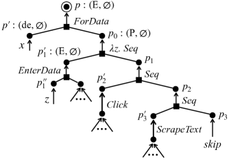
Figure 13. Illustration of one potential $\mathcal{A}_{s}$ given by SpeculateFTA for the initial FTA from Figure 10.

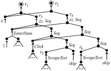
Figure 14. Illustration of a part of $\mathcal{A}_{e}$ returned by EvaluateFTA for $\mathcal{A}_{s}$ from Figure 14.

4.4. FTA Initialization

Now let us circle back and describe the FTA initialization procedure, which we note is specific to PBD and web automation. Figure 15 shows the key initialization rule that constructs, from action trace $[a_{1},\cdots,a_{m}]$ and DOM trace $[\pi_{1},\cdots,\pi_{m}]$, $m$ consecutive Seq transitions in the initial FTA $\mathcal{A}$. In particular, all $q_{i}$ ($i\in[0,m]$) states have grammar symbol P, and all $q^{\prime}_{i}$ ($i\in[1,m]$) states have E. Each Seq transition $\delta_{i}$ ($i\in[1,m]$) connects $q^{\prime}_{i}$ and $q_{i}$ to $q_{i-1}$, forming $m$ consecutive Seq transitions. The footprint in $q_{i}$ means that all programs in $\textit{SubFTA}(q_{i},\mathcal{A})$ yield $[a_{i+1},\cdots,a_{m}],\texttt{[]}$ under context $[\pi_{i+1},\cdots,\pi_{m}],\Gamma$. Similarly, for each $q^{\prime}_{i}$, it maps the context $[\pi_{i},\cdots,\pi_{m}],\Gamma$ to $[a_{i}],[\pi_{i+1},\cdots,\pi_{m}]$.

In addition to Seq, we also have transitions for statements (like Click and ScrapeText) and selectors. The following rule shows how to construct transitions for Click and its candidate selectors, from action trace $[a_{1},\cdots,a_{m}]$, DOM trace $[\pi_{1},\cdots,\pi_{m}]$, and input data $I$.

$$\small\begin{array}[]{c}\mkern-2.0mu\displaystyle\frac{\begin{array}[]{c}i\in[1,m]\ \ \ \ a_{i}=\emph{Click}({\raisebox{1.0pt}{$\chi$}})\ \ \ \ \pi_{i}\vdash se:{\raisebox{1.0pt}{$\chi$}}\ \ \ \ \Gamma=\{x\mapsto I\}\\ q^{\prime}_{i}=\textit{MkState}\Big{(}\textsf{E},\big{\{}[\pi_{i},\cdots,\pi_{m}],\Gamma\mapsto[a_{i}],[\pi_{i+1},\cdots,\pi_{m}]\big{\}}\Big{)}\ \ \ \ q^{{\prime\mkern-2.0mu\prime\mkern-3.0mu}}_{i}=\textit{MkState}\Big{(}\textsf{se},\big{\{}\pi_{i},\Gamma\mapsto{\raisebox{1.0pt}{$\chi$}}\big{\}}\Big{)}\\ \delta^{\prime}_{i}=\emph{Click}(q^{{\prime\mkern-2.0mu\prime\mkern-3.0mu}}_{i})\rightarrow q^{\prime}_{i}\ \ \ \ \delta^{{\prime\mkern-2.0mu\prime\mkern-3.0mu}}_{i}=se\rightarrow q^{{\prime\mkern-2.0mu\prime\mkern-3.0mu}}_{i}\end{array}}{\vphantom{,}q^{\prime}_{i},q^{{\prime\mkern-2.0mu\prime\mkern-3.0mu}}_{i}\in Q\ \ \ \ \delta^{\prime}_{i},\delta^{{\prime\mkern-2.0mu\prime\mkern-3.0mu}}_{i}\in\Delta}\mkern-2.0mu\end{array}$$

Intuitively, this rule states: given a Click action $a_{i}$ (with a full selector expression $\chi$) that is performed on DOM $\pi_{i}$, for any candidate selector $se$ that refers to the same DOM element on $\pi_{i}$ as $\chi$, we create a transition for $se$. This is exactly why Figure 10 has multiple selectors in the dashed circle around each ${\raisebox{1.0pt}{$\chi$}}_{i}$. The construction rules for other actions are very similar; we skip the details here.

$\displaystyle\footnotesize\centering\begin{array}[]{l}\mkern-2.0mu\displaystyle\frac{\begin{array}[]{ll}\Gamma=\{x\mapsto I\}\\ q_{0}=\textit{MkState}\Big{(}\textsf{P},\big{\{}[\pi_{1},\cdots,\pi_{m}],\Gamma\mapsto[a_{1},\cdots,a_{m}],\texttt{[]}\big{\}}\Big{)}&q^{\prime}_{1}=\textit{MkState}\Big{(}\textsf{E},\big{\{}[\pi_{1},\cdots,\pi_{m}],\Gamma\mapsto[a_{1}],[\pi_{2},\cdots,\pi_{m}]\big{\}}\Big{)}\\ q_{1}=\textit{MkState}\Big{(}\textsf{P},\big{\{}[\pi_{2},\cdots,\pi_{m}],\Gamma\mapsto[a_{2},\cdots,a_{m}],\texttt{[]}\big{\}}\Big{)}&q^{\prime}_{2}=\textit{MkState}\Big{(}\textsf{E},\big{\{}[\pi_{2},\cdots,\pi_{m}],\Gamma\mapsto[a_{2}],[\pi_{3},\cdots,\pi_{m}]\big{\}}\Big{)}\\ \cdots&\cdots\\ q_{m}=\textit{MkState}\Big{(}\textsf{P},\big{\{}\texttt{[]},\Gamma\mapsto\texttt{[]},\texttt{[]}\big{\}}\Big{)}&q^{\prime}_{m}=\textit{MkState}\Big{(}\textsf{E},\big{\{}[\pi_{m}],\Gamma\mapsto[a_{m}],\texttt{[]}\big{\}}\Big{)}\\ \delta_{1}=\emph{Seq}(q^{\prime}_{1},q_{1})\rightarrow q_{0}\ \cdots\ \delta_{m}=\emph{Seq}(q^{\prime}_{m},q_{m})\rightarrow q_{m-1}\end{array}}{\vphantom{,}q_{0},\cdots,q_{m},q^{\prime}_{1},\cdots,q^{\prime}_{m}\in Q\ \ \ \ \delta_{1},\cdots,\delta_{m}\in\Delta\ \ \ \ q_{0}\in Q_{f}}\mkern-2.0mu\end{array}\@add@centering$

Figure 15. Key FTA initialization rule, given action trace $[a_{1},\cdots,a_{m}]$ and DOM trace $[\pi_{1},\cdots,\pi_{m}]$.

1: procedure SpeculateForData($[\delta_{1},\cdots,\delta_{2l}],\Delta$)

2: input: Each $\delta_{i}$ is of the form $\delta_{i}=\emph{Seq}(q^{\prime}_{i},q_{i})\rightarrow q_{i-1}$, $i\in[1,2l]$. $\Delta$ is a set of transitions.

3: output: FTA with final state $p$ and transitions $\Delta^{\prime}$, which represents a set of speculated ForData loops.

4:$U_{1}:=\textsc{AntiUnify}\textsc{ForData}(q^{\prime}_{1},q^{\prime}_{l+1},\Delta)$;   $\cdots$;   $U_{l}:=\textsc{AntiUnify}\textsc{ForData}(q^{\prime}_{l},q^{\prime}_{2l},\Delta)$;

5:$U:=U_{1}\cup\cdots\cup\ U_{l}$;   $(\{p^{\prime}_{1}\},\Delta^{\prime}_{1}):=\textsc{Parametrize}(q^{\prime}_{1},\Delta,U)$;   $\cdots$;   $(\{p^{\prime}_{l}\},\Delta^{\prime}_{l}):=\textsc{Parametrize}(q^{\prime}_{l},\Delta,U)$;

6:create fresh states $p_{0}(\textsf{P},\emptyset),\cdots,p_{l}(\textsf{P},\emptyset)$, and $p^{\prime}(\textsf{de},\emptyset),p(\textsf{E},\emptyset)$;

7:$\Delta^{\prime}:=$     $\{\emph{ForData}(p^{\prime},p_{0})\rightarrow p\}$ $\cup\ \{\emph{Seq}(p^{\prime}_{i},p_{i})\rightarrow p_{i-1}\ |\ i\in[1,l]\}$

8:        $\cup\ \{u\rightarrow p^{\prime}\ |\ u\in U\}$ $\triangleright$ Transitions corresponding to anti-unifiers

9:        $\cup\ \ \Delta^{\prime}_{1}\cup\cdots\cup\Delta^{\prime}_{l}$; $\triangleright$ Transitions constructed from parametrization

10:return $\big{(}\{p\},\Delta^{\prime}$ );

Algorithm 2: Algorithm for SpeculateForData that speculates an FTA of ForData loops.

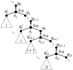
Figure 16. Illustration of the $2l$ consecutive transitions $\delta_{1},\cdots,\delta_{2l}$ (line 7, Algorithm 1).

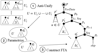
Figure 17. Illustration of Algorithm 2, given the $2l$ transitions $\delta_{1},\cdots,\delta_{2l}$ from Figure 17.

4.5. Speculating FTAs

Section 4.3 assumed a given speculated FTA $\mathcal{A}_{s}$. In this section, let us unpack the SpeculateFTA algorithm that infers $\mathcal{A}_{s}$. Here, $\mathcal{A}_{s}$ is an FTA that contains candidate loops (potentially nested).

Figure 17 illustrates how to speculate candidate ForData loops from the $2l$ consecutive transitions $\delta_{1},\cdots,\delta_{2l}$ (illustrated in Figure 17). Algorithm 2 describes the algorithm more formally. We suggest readers simultaneously looking at Figures 17, Figure 17 and Algorithm 2.

The first step is anti-unification (line 4): for all $i\in[1,l]$, we synchronously traverse $\textit{SubFTA}(q^{\prime}_{i},\mathcal{A})$ and $\textit{SubFTA}(q^{\prime}_{l+i},\mathcal{A})$, and compute a set $U_{i}$ of anti-unifiers. For ForData, an anti-unifier $u$ is simply a data expression that ForData may iterate over. The second step is parametrization (lines 5): for all anti-unifiers from $U$, we traverse $\textit{SubFTA}(q^{\prime}_{i},\mathcal{A})$ ($i\in[1,l]$) and build a new FTA with final state $p^{\prime}_{i}$ and transitions $\Delta^{\prime}_{i}$. The third and last step is to construct the final speculated FTA $\mathcal{A}_{s}$ (line 6-7). Each state in $\mathcal{A}_{s}$ is annotated with an empty footprint, because we are yet to evaluate any programs. In other words, $\mathcal{A}_{s}$ is purely a syntactic compression without using any OE at all.

We refer interested readers to the appendix for a more complete description of the speculation algorithm that handles other types of loops. In what follows, we explain our anti-unification and parametrization algorithms.

$\displaystyle\centering\begin{array}[]{l}(1)\ \mkern-2.0mu\displaystyle\frac{\begin{array}[]{c}f\in\{\emph{Click},\emph{ScrapeText},\emph{ScrapeLink},\emph{Download},\emph{EnterData}\}\\ f(\cdots,q^{\prime}_{i},\cdots)\rightarrow q_{i}\in\Delta\ \ \ \ \Delta\vdash q^{\prime}_{1},q^{\prime}_{2}\twoheadrightarrow u\end{array}}{\vphantom{,}\Delta\vdash q_{1},q_{2}\twoheadrightarrow u}\mkern-2.0mu\par\ \ \ \ \ \par(2)\ \mkern-2.0mu\displaystyle\frac{\begin{array}[]{c}f\in\{\emph{ForData},\emph{ForSelectors}\}\\ f(q^{\prime}_{i},\cdots)\rightarrow q_{i}\in\Delta\ \ \ \ \Delta\vdash q^{\prime}_{1},q^{\prime}_{2}\twoheadrightarrow u\end{array}}{\vphantom{,}\Delta\vdash q_{1},q_{2}\twoheadrightarrow u}\par\mkern-2.0mu\\[10.0pt] (3)\ \mkern-2.0mu\displaystyle\frac{\begin{array}[]{c}de_{i}\rightarrow q_{i}\in\Delta\\ \vdash de_{1},de_{2}\twoheadrightarrow u\end{array}}{\vphantom{,}\Delta\vdash q_{1},q_{2}\twoheadrightarrow u}\mkern-2.0mu\par\par\par\ \ \par(4)\ \mkern-2.0mu\displaystyle\frac{\begin{array}[]{c}\\ de_{i}=de^{\prime}\big{[}z\mapsto de[i]\big{]}\end{array}}{\vphantom{,}\vdash de_{1},de_{2}\twoheadrightarrow de}\mkern-2.0mu\par\par\ \ \par(5)\ \mkern-2.0mu\displaystyle\frac{\begin{array}[]{c}se_{i}\rightarrow q_{i}\in\Delta\\ \vdash se_{1},se_{2}\twoheadrightarrow u\end{array}}{\vphantom{,}\Delta\vdash q_{1},q_{2}\twoheadrightarrow u}\mkern-2.0mu\par\ \ \par(6)\ \mkern-2.0mu\displaystyle\frac{\begin{array}[]{c}\oplus\in\{/,\mkern 0.0mu/\mkern-5.0mu/\mkern 0.0mu\}\\ se_{i}=se^{\prime}\big{[}y\mapsto se\oplus\psi[k+i-1]\big{]}\end{array}}{\vphantom{,}\vdash se_{1},se_{2}\twoheadrightarrow se\oplus\psi[k]}\par\mkern-2.0mu\end{array}\@add@centering$

Figure 18. Anti-unification rules.

$\displaystyle\centering\begin{array}[]{l}(1)\ \mkern-2.0mu\displaystyle\frac{\begin{array}[]{c}\begin{array}[]{c}f(\cdots,q^{\prime},\cdots)\rightarrow q\in\Delta\ \ \ \ \oplus\in\{/,\mkern 0.0mu/\mkern-5.0mu/\mkern 0.0mu\}\ \ \ \ u\in U\\ u\oplus se\rightarrow q^{\prime}\in\Delta\end{array}\end{array}}{\vphantom{,}y\oplus se\rightarrow M(q^{\prime})\in\Delta^{\prime}}\mkern-2.0mu\par\hskip 30.0pt\par(2)\ \mkern-2.0mu\displaystyle\frac{\begin{array}[]{c}f(\cdots,q^{\prime},\cdots)\rightarrow q\in\Delta\ \ \ \ u\in U\\ u[1]\rightarrow q^{\prime}\in\Delta\end{array}}{\vphantom{,}z\rightarrow M(q^{\prime})\in\Delta^{\prime}}\par\par\mkern-2.0mu\end{array}\@add@centering$

Figure 19. Parametrization rules.

Anti-unification. Given two states $q_{1},q_{2}$ from FTA $\mathcal{A}$ with transitions $\Delta$, anti-unification traverses expressions in $\textit{SubFTA}(q_{1},\mathcal{A})$ and $\textit{SubFTA}(q_{2},\mathcal{A})$ in a synchronized fashion, and returns a set $U$ of anti-unifiers that may be iterated over by the speculated loops. In particular:

$$\begin{array}[]{c}\textsc{AntiUnify}(q_{1},q_{2},\Delta)=U=\{\ u\ |\ \Delta\vdash q_{1},q_{2}\twoheadrightarrow u\ \}\end{array}$$

That is, $u\in U$ if there is an anti-unifier $u$ for $q_{1},q_{2}$ given $\Delta$. Figure 18 presents the detailed rules. Rule (1) says that, to anti-unify $q_{1},q_{2}$ with incoming transition $f$, we anti-unify the argument states $q^{\prime}_{1},q^{\prime}_{2}$. Rule (2) does the same but for loops: we anti-unify expressions (i.e., the first argument) being looped over. Rules (3) and (4) concern the anti-unification of data expressions — the idea is to look for an increment pattern beginning with 1. Rules (5) and (6) anti-unify selector expressions, where it uses a more flexible pattern that allows starting from $k$ (not necessarily $k=1$).

Example 4.3.

Consider states $q^{\prime}_{1}$ and $q^{\prime}_{4}$ in $\mathcal{A}$ from Figure 10. The anti-unifier for $q^{\prime}_{1},q^{\prime}_{4}$ is $x$.

Parametrization. Given all anti-unifiers $U$ and a state $q$ from $\mathcal{A}$ with transitions $\Delta$, Parametrize constructs from $\textit{SubFTA}(q,\mathcal{A})$ a fresh new $\mathcal{A}^{\prime}$ (with transitions $\Delta^{\prime}$ and final state $q^{\prime}$) in two steps.

First, we make a fresh new copy of each state from $\textit{SubFTA}(q,\mathcal{A})$, keeping the same grammar symbol and but resetting the footprint to empty. This results in a mapping $M$ that maps every state in $\textit{SubFTA}(q,\mathcal{A})$ to a state in $\mathcal{A}^{\prime}$. Therefore, for each transition $f(q_{1},\cdots,q_{n})\rightarrow q_{0}\in\Delta$, we have $f\big{(}M(q_{1}),\cdots,M(q_{n})\big{)}\rightarrow M(q_{0})\in\Delta^{\prime}$.

Then, we add new transitions labeled with parametrized selector/data expressions to $\mathcal{A}^{\prime}$, given each anti-unifier $u\in U$, mapping $M$, and the state $q$ from $\mathcal{A}$ with transitions $\Delta$. In other words, the actual parametrization takes place in this step. Figure 19 presents our parametrization rules. Rule (1) parametrizes any transition in $\Delta$ that uses a selector expression of the form $u\oplus se$; that is, this selector uses the anti-unifier $u$ as a prefix. This rule adds a new transition with $u$ being replaced by variable $y$ which points to state $M(q^{\prime})$. Rule (2) parametrizes data expressions in a similar manner.

Example 4.4.

Consider the initial FTA $\mathcal{A}$ in Figure 10. Consider the anti-unifier $x$ from Example 4.3. Let us explain how to parametrize state $q^{\prime}_{1}$ from $\mathcal{A}$, given anti-unifier $x$, to generate state $p^{\prime}_{1}$ in $\mathcal{A}_{s}$ from Figure 14. We first make a copy of $\textit{SubFTA}(q^{\prime}_{1},\mathcal{A})$: for example, the copy of $q^{\prime}_{1}$ is $p^{\prime}_{1}$; that is, $M(q^{\prime}_{1})=p^{\prime}_{1}$. Then, we invoke Rule (2) from Figure 19 with $f$ being EnterData. This yields a new transition $z\rightarrow M(q^{{\prime\mkern-2.0mu\prime\mkern-3.0mu}}_{1})$ where $p^{{\prime\mkern-2.0mu\prime\mkern-3.0mu}}_{1}=M(q^{{\prime\mkern-2.0mu\prime\mkern-3.0mu}}_{1})$, which indeed appears in $\mathcal{A}_{s}$ in Figure 14.

Constructing $\mathcal{A}_{s}$. Finally, lines 6-7 connect the created states and transitions, as shown in Figure 17.

4.6. Merging FTAs

Let us explain the last two procedures in Algorithm 1.

Figure 20. MergeFTAs.

Merging $\mathcal{A}_{e}$ into $\mathcal{A}$. Intuitively, MergeFTAs (line 11) incorporates loops from $\mathcal{A}_{e}$ into $\textit{SubFTA}(q_{0},\mathcal{A})$. Figure 20 illustrates how this works. We first construct a state $q^{\prime}$ and a Seq transition $\delta$ that connects a final state $q$ from $\mathcal{A}_{e}$ and $q^{\prime}$ to $q_{0}$. In particular, $q^{\prime}$ has grammar symbol P and is associated with the following footprint:

$$\small\centering\left\{\begin{array}[]{c}\Pi^{\prime}_{1},\Gamma\mapsto A^{\prime}_{2},\Pi^{\prime}\par\ \Big{|}\ \par\begin{array}[]{l}\Pi,\Gamma\mapsto A^{\prime},\Pi^{\prime}\ \in\textit{Footprint}(q_{0})\\ \Pi,\Gamma\mapsto A^{\prime}_{1},\Pi^{\prime}_{1}\in\textit{Footprint}(q)\\ A^{\prime}_{1}\mkern 0.0mu\texttt{+}\mkern-1.0mu\texttt{+}\mkern 1.0muA^{\prime}_{2}=A^{\prime}\end{array}\end{array}\right\}\vspace{5pt}\@add@centering$$

In other words, $q^{\prime}$ is constructed based on footprints from $q_{0}$ and $q$, according to Seq’s semantics. Note the constraint $A^{\prime}_{1}\mkern 0.0mu\texttt{+}\mkern-1.0mu\texttt{+}\mkern 1.0muA^{\prime}_{2}=A^{\prime}$: we only keep loops in $\textit{SubFTA}(q,\mathcal{A}_{e})$ that yield a prefix of $A^{\prime}$, because otherwise $A^{\prime}_{1}$ is not a reachable context for $q$, at least not so in this case. For such final states $q$ of $\mathcal{A}_{e}$, we create the aforementioned $q^{\prime}$ and $\delta$, and add $\delta$ together with all transitions in $\mathcal{A}_{e}$ to the set of transitions of $\mathcal{A}$. Observe that, if $q^{\prime}$ already exists in $\mathcal{A}$, then MergeFTAs effectively connects $q$ and an existing state $q^{\prime}$ in $\mathcal{A}$ to $q_{0}$ which is also in $\mathcal{A}$.

Ranking. The Ranking procedure (line 12) is fairly straightforward. It first runs EvaluateFTA on $\mathcal{A}$ using $\Pi,\{x\mapsto I\}$ as the context. Note that the last DOM $\pi_{m+1}$ in $\Pi$ does not have a demonstrated action in the input action trace $A$, because our goal is to use the synthesized program $P$ to automate the unseen actions. EvaluateFTA gives $\mathcal{A}^{\prime}$ containing programs with different predicted actions $a_{m+1}$. We pick a program $P$ with the smallest size and return $P$ as the final synthesized program.

4.7. Soundness and Completeness

Theorem 4.5.

Given action trace $A$, DOM trace $\Pi$ and input data $I$, our synthesis algorithm always terminates. Moreover, if there exists a program in our grammar (shown in Figure 8) that generalizes $A$ (given $\Pi$ and $I$) and satisfies the condition that (1) every loop has at least two iterations exhibited in $A$ and (2) its final expression is a loop, then our synthesis algorithm (shown in Algorithm 1) would return a program that generalizes $A$ (given $\Pi$ and $I$) upon FTA saturation.

4.8. Interactive Synthesis with Incremental FTA Construction

Interactive programming-by-demonstration. Same as WebRobot (Dong et al., 2022), our synthesis technique can also be applied in an interactive setting: given an action trace $A_{m}=[a_{1},\cdots,a_{m}]$ and a DOM trace $\Pi_{m}=[\pi_{1},\cdots,\pi_{m+1}]$, we synthesize a program $P_{m}$ that produces $a^{\prime}_{m+1}$ given $\Pi_{m}$. If this prediction $a^{\prime}_{m+1}$ is not intended, the user would manually demonstrate a correct $a_{m+1}$. This leads to new traces $A_{m+1}=[a_{1},\cdots,a_{m+1}]$ and $\Pi_{m+1}=[\pi_{1},\cdots,\pi_{m+2}]$, both of which are fed to our algorithm again. This process repeats until the user obtains an intended program.

Incremental FTA construction. We incrementalize our Algorithm 1 based on the interactive setup. Given $A_{m+1}$ and $\Pi_{m+1}$, and given FTA $\mathcal{A}_{m}$ constructed from $A_{m}$ and $\Pi_{m}$, we still build $\mathcal{A}_{m+1}$ with the same guarantee as in Algorithm 1 but not from scratch. Our key insight is that we can re-use the validated loops from $\mathcal{A}_{m}$, but we need to evaluate them against $\Pi_{m+1}$ as some of them may not reproduce $A_{m+1}$. Essentially, our incremental algorithm is still based on guess-and-check, but we have a second type of speculation that directly takes sub-FTAs from $\mathcal{A}_{m}$ as speculated FTAs — this generates high-quality speculated FTAs more efficiently. $\mathcal{A}_{m+1}$ is still initialized in the same way but this time using $A_{m+1}$ and $\Pi_{m+1}$. We still perform SpeculateFTA and EvaluateFTA on $\mathcal{A}_{m+1}$ but in a much smaller scope this time. That is, $\delta_{2l}$ must involve $a_{m+1}$, because otherwise $\mathcal{A}_{m}$ had already considered it. The MergeFTAs and Ranking procedures remain the same.

5. Evaluation

This section describes a series of experiments designed to answer the following questions:

• RQ1: Can Arborist efficiently synthesize programs for challenging web automation tasks? How does it compare against state-of-the-art techniques?

• RQ2: How necessary is it to use an expressive language in order to have a generalizable program? In particular, is it important to consider a large space of candidate selectors?

• RQ3: How does Arborist scale with respect to the number of candidate selectors considered?

• RQ4: How useful are various ideas proposed in this work?

Web automation tasks. To answer these questions, we construct a collection of web automation tasks from two different sources. First, we include all 76 tasks that were used to evaluate WebRobot: details about these tasks can be found in (Dong et al., 2022). Second, we curate 55 new tasks, each of which has an English description of the task logic over one or more websites. All of our new tasks are curated based on real-life problems (e.g., those from the iMacros forum) and involve modern, popular websites (such as Amazon, UPS, Craigslist, IMDb) with complex webpages, whereas many of WebRobot’s benchmarks involve legacy websites. These new websites have deeply nested DOM structures which would require searching with a significantly larger space of candidate selectors. In particular, all 131 tasks involve data extraction, 45 of them involve data entry, 80 require navigation across webpages, and 48 involve pagination. Some of these tasks involve multiple types: for instance, 31 of them involve data entry, data extraction, and webpage navigation.

Ground-truth Selenium programs. For each task, we obtain a ground-truth automation program $P_{\emph{gt}}$ (using the Selenium WebDriver framework). In particular, we reuse the 76 ground-truth Selenium programs from WebRobot, and manually write 55 programs for our new tasks. On average, these Selenium programs consist of 43 lines of code, with a max of 147 lines. In general, it takes about half an hour to a few hours for us to write up an automation program, depending on the complexity of webpages and the task logic.

Benchmarks. In our evaluation, a benchmark is defined as a tuple $(A,\Pi,I)$, where $A$ is an action trace, $\Pi$ is a DOM trace, and $I$ is input data. We obtain one benchmark for each task by running the corresponding $P_{\emph{gt}}$ in the browser (given input data $I$ if $P_{\emph{gt}}$ involves data entry) — during execution, we record the trace $A=[a_{1},\cdots,a_{m}]$ of actions that $P_{\emph{gt}}$ executes as well as $A$’s corresponding DOM trace $\Pi=[\pi_{1},\cdots,\pi_{m}]$. Here, $a_{i}$ is an action performed on $\pi_{i}$. Note that selectors in actions are recorded as full XPath expressions.

Candidate selectors. For any full XPath selector $\chi$ in an action $a_{i}$, we also record a set $S$ of candidate selectors for $\chi$. In particular, a candidate selector $se$ is a concrete selector expression (i.e., without variable $y$) from our grammar (see Figure 8) that locates the same DOM element on $\pi_{i}$ as $\chi$. In other words, $se$ evaluates to $\chi$ given $\pi_{i}$, or more formally, $\pi_{i}\vdash se:{\raisebox{1.0pt}{$\chi$}}$. As mentioned in Example 1 and Section 4.2, it is important to consider candidate selectors, since full XPath expressions typically do not generalize. Candidate selectors also affect the overall search space, as explained below.

Program space. In this work, the search space of programs for a benchmark with action trace $A$ is defined jointly by the grammar from Figure 8 and the candidate selectors for all actions in $A$. This is because Figure 8 does not specify a priori the space of selectors $se$ and predicates $\psi$. Instead, they are defined once the traces $A$ and $\Pi$ are given: e.g., the space for $se$ includes all candidate selectors. It is very hard (if not impossible) to define this space a priori without the DOMs. Obviously, the overall search space of programs grows when we consider more candidate selectors.

5.1. RQ1: Can Arborist Automate Challenging Web Automation Tasks?

In this section, we evaluate Arborist against three metrics: (i) how many tasks it can successfully synthesize intended programs for, (ii) how much synthesis time it takes, and (iii) how many user-demonstrated actions it requires in order to synthesize intended programs. In other words, we evaluate Arborist’s effectiveness, efficiency, and generalization power. We also compare Arborist against the state-of-the-art, especially on our new tasks that are more challenging.

Setup. We use the same setup from the WebRobot paper (Dong et al., 2022). In particular, given a benchmark with $A$ and $\Pi$ that have $m$ actions and DOMs respectively, we create $m-1$ tests. The $k$th test consists of an action trace $A_{k}=[a_{1},\cdots,a_{k}]$ and a DOM trace $\Pi_{k}=[\pi_{1},\cdots,\pi_{k},\pi_{k+1}]$. For each action, we consider all candidate selectors in our grammar with at most 3 predicates. For example, a[1]/b[2] uses 2 predicates and therefore is included, but c/d/a[1]/b[2] is not considered even if it can also locate the same DOM element. We run Arborist in a way to simulate an interactive PBD process, same as how WebRobot was evaluated. That is, we feed all tests to Arborist in sequence: we run Arborist on the $k$-th test (with $A_{k}$ and $\Pi_{k}$), obtain a synthesized program $P_{k}$, and check if $P_{k}$ predicts $a_{k+1}$ (i.e., $P_{k}$ yields $A_{k+1}$ given $\Pi_{k}$). If not, $a_{k+1}$ is counted as a user-demonstrated action; otherwise, $a_{k+1}$ can be correctly predicted and thus is not counted. We always count the first action $a_{1}$ as user-demonstrated. Furthermore, for each test we use a 1-second timeout and record the time it takes to return $P_{k}$. We run Arborist incrementally (as described in Section LABEL:sec:alg:key-optimizations) in this experiment: for each test, it resumes synthesis based on FTAs from previous tests/iterations. Finally, we inspect if the synthesized program $P_{m-1}$ (in the last iteration) is an intended program: if so, the corresponding benchmark is counted as solved; otherwise, unsolved.

Baselines. Among three baselines, we focus on the following two.

• WebRobot, which is the original tool from the WebRobot work (Dong et al., 2022). We note that, while its underlying algorithm is complete in theory, the implementation is not. For example, it restricts the number of parametrized selectors (to five) when parametrizing actions during speculation. These heuristics seemed to help avoid excessively slowing down the search, without severely hindering the completeness for those tasks considered in the WebRobot work.

• WebRobot-extended, which is an adapted version of WebRobot that uses the extended language from Figure 8 (which allows ForSelectors with $i\geq 1$). In this experiment, we range $i$ from $1$ to $3$. This baseline still keeps all heuristics from WebRobot (i.e., its search is incomplete).

We use the same space of candidate selectors as Arborist for these two baselines. The third baseline is Helena (Chasins, 2019), which is also a PBD-based web automation tool.

RQ1 take-away: • Arborist can synthesize intended programs for 93.9% of our benchmarks. • It typically takes Arborist subseconds to synthesize programs from demonstration. • Arborist uses a median of 12 user-demonstrated actions to generalize. • Arborist can solve more benchmarks using less time than state-of-the-art techniques.

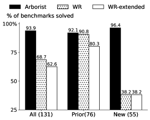
(a) Percentage of benchmarks solved.

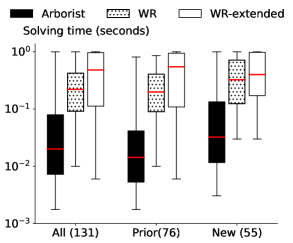
(b) Synthesis times for solved benchmarks.

Figure 21. RQ1 main results. WR stands for WebRobot, and WR-extended means WebRobot-extended.

Main results. Figure 21 summarizes the main results for both Arborist and baselines: Figure 21(a) shows the percentage of benchmarks where intended programs can be synthesized, and Figure 21(b) reports the distribution of their corresponding synthesis times. Note that for both figures, we show both the aggregated data across all 131 benchmarks, and separately for prior and new tasks.

Let us inspect Figure 21(a) first. Across all 131 benchmarks, Arborist can synthesize an intended program for 93.9% (i.e., 123) of them, whereas baselines solve at most 68.7% (i.e., 90). This is a large gap, because baselines solve significantly fewer new tasks (which are very challenging): in particular, Arborist can solve 53 out of 55 (i.e., 96.4%), which is 2.5x more than that for baselines (i.e., 21/38.2%). These new tasks involve complex webpages and task logics, which require using nested loops and searching for selectors with more predicates in a larger space. This makes them significantly more challenging than prior tasks; as a result, WebRobot’s underlying enumeration-based algorithm fundamentally cannot scale to this level of complexity. For prior tasks (total 76) in the WebRobot paper (which baselines were developed and engineered on), Arborist still outperforms baselines by one more benchmark. It turns out this benchmark involves two loops that require the start index to be 2 and 3, which cannot be expressed in WebRobot’s original language. WebRobot-extended, however, solves this benchmark, since it uses a richer language. Arborist uses the same (extended) language, and therefore is able to synthesize an intended program as well.

In addition to solving a strict superset of benchmarks than baselines, Arborist is also significantly faster. Figure 21(b) reports statistics of the synthesis times. In particular, for each solved benchmark, we record the maximum synthesis time across all tests, and report the distribution of these times. For each tool, Figure 21(b) presents the quartile statistics of synthesis times. Across all 123 benchmarks solved by Arborist, 120 of them do not even use up the 1-second timeout. In contrast, baselines solve fewer benchmarks and time out on 15 benchmarks. Recall that both baselines have internal heuristics which unsoundly prune search space for faster search. We tested variants of them with these heuristics removed: the best one can solve 55 benchmarks, with 46 timeouts. In other words, for many benchmarks, baselines cannot exhaust the entire search space, although they stumped upon a correct program before timeout. With a longer timeout of 10 seconds, baselines can only solve 9 more benchmarks. On the other hand, with 1-second timeout, Arborist times out on 3 benchmarks — they all require doubly nested loops and are among the most challenging ones. Arborist solves them all (albeit reaching timeout), while baselines solve two.

Arborist uses a median of 12 user-demonstrated actions, which is in line with that for WebRobot. This is reasonable, as we use the same search space for all tools in this experiment. While Arborist searches more programs than baselines (which oftentimes time out and hence search a small subset), our simple ranking heuristics seem to be quite effective at selecting generalizable programs.

Discussion. Arborist failed to solve 8 benchmarks, including 6 from prior work (due to limitations of the web automation language, as also explained in the WebRobot paper) and 2 new ones (which can be solved using a 10-second timeout). Careful readers may wonder why WebRobot-extended solves fewer benchmarks than WebRobot, albeit using a richer language. This is due to the poor performance of its underlying enumeration-based algorithm: using a 1-second timeout, WebRobot-extended cannot even find intended programs for some benchmarks that WebRobot solves.

Detailed results. Recall that Arborist internally has two key modules — namely, SpeculateFTA and EvaluateFTA — which typically use most of the running time. Among them, on average, the former takes 20% of the time, and the latter uses 80%, across all benchmarks. The final FTA has an average of 1714 states. The final synthesized programs on average have 6 expressions, and the largest one has 20. Among these programs, 76 use at least one doubly-nested loop, and 12 involve at least a three-level loop.

Arborist vs. Helena. Among the 76 WebRobot benchmarks, Helena’s PBD technique was able to synthesize intended programs from demonstrations (provided by us manually) for 13 benchmarks. For the 55 new tasks, Helena solved 11. By contrast, Arborist solved 70 and 53 respectively.

5.2. RQ2: How Important Is It To Consider Many Candidate Selectors?

The search space considered in RQ1 uses the grammar from Figure 8 with candidate selectors of size up to three (measured by the number of predicates). This is a quite expressive language containing at least one generalizable program for over 93% of our tasks (as Arborist was able to solve them). However, one might ask: is this high expressiveness really necessary? This is an important question, because if not, advanced synthesis techniques like Arborist may not be necessary in practice.

Setup. In this section, we investigate the impact of candidate selectors on the expressiveness of the resulting search space: that is, given a set $S$ of candidate selectors, whether or not the corresponding program space has at least one generalizable program. We choose to focus on candidate selectors in this experiment, because prior work (Dong et al., 2022) has already shown the necessity of operators from the grammar in Figure 8.

More specifically, given a benchmark with action trace $A$, for each $a_{i}$ with full XPath selector $\chi$, we use the following ways to construct the set $S$ of candidate selectors for $a_{i}$.

• $S$ includes all candidate selectors for $\chi$ up to a certain size. This is perhaps the simplest heuristic that one can design; RQ1 uses 3 as the max size which was shown to be sufficient for most of our benchmarks. Therefore, in this experiment, we vary the max size from 1 to 3, and investigate how it impacts the expressiveness. For each size, we run Arborist using the corresponding $S$, and record the number of benchmarks solved. Here, “solved” means an intended program can be found by Arborist, which is a witness that corresponding search space is expressive enough.

• $S$ contains candidate selectors sampled (uniformly at random) from all candidate selectors of size up to 3. We vary $|S|$ from 1 to 1500. For each $|S|$, we run Arborist with the corresponding $S$ and record the number of benchmarks solved; we repeat this 8 times. This gives us a finer-grained, more continuous view of the impact of candidate selectors.

While one could certainly craft other heuristics for constructing $S$, we do not consider them, because (i) it is impossible to enumerate all heuristics in the first place, and (ii) human-crafted heuristics from prior work (Chasins et al., 2018; Dong et al., 2022) have shown to be not as effective especially for challenging tasks. Another note is that, since we use Arborist merely as a means to check if the search space has a generalizable program, the synthesis time is not relevant in this experiment.

For each benchmark with a given $S$, we run Arborist incrementally until it reaches the end of the action trace, same as in RQ1. However, in RQ2, we use 10 seconds as the timeout per iteration, rather than 1 second from RQ1 — this allows Arborist to exhaustively search the program space such that we can more confidently conclude on its expressiveness. If the final synthesized program is intended, we count it as solved (meaning the corresponding search space is expressive enough).

RQ2 take-away: In general, an expressive search space should consider a large number of selectors (at least at the level of hundreds) for each webpage.

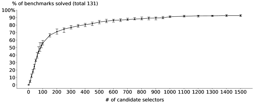
Figure 22. RQ2 results. Given X candidate selectors (sampled uniformly at random from all candidate selectors of size up to 3), we have Y benchmarks whose search space is confirmed to contain an intended program.

Results. If using only the full XPath expressions from the input action trace, Arborist manages to solve 46 benchmarks (out of 131 total), while terminating on the remaining 85 without synthesizing an intended program. That is, the search spaces of the 85 benchmarks are exhausted before timeout. This confirms that full XPath expressions typically do not generalize, and we need to consider more candidate selectors in order to solve more tasks. If we additionally include all candidate selectors of size 1, the number of solved benchmarks bumps up to 87, which is 66% of all benchmarks. Arborist does not reach timeout for any of the rest, indicating the need to consider more selectors. Further including all candidate selectors of size 2 allows Arborist to solve 122 benchmarks, which is quite close to our results in RQ1. Again, no timeout is observed on the remaining benchmarks. We note that the selector space at this point is already quite large: on average, we have 305 selectors of size up to two (in our grammar) per DOM across our benchmarks; the median and max are 321 and 385 respectively. In other words, using a simple size-based heuristic, we necessarily need to consider multiple hundreds of candidate selectors per DOM, in order to automate a decent number of tasks. Finally, when considering all candidate selectors of size up to 3 (same as in RQ1), 125 benchmarks are confirmed to admit intended programs; no timeouts observed. The remaining 6 benchmarks, upon manual inspection, cannot be solved by Arborist’s language (to our best knowledge). While encouraging, this high expressiveness comes at the cost of searching among an average of 7627 selectors per DOM, with the median and max being 8066 and 9649, across all our benchmarks.

Figure 22 presents a finer-grained view of how the expressiveness increases when we range the number of candidate selectors from 0 to 1500 using a small increment. The x-axis is the number of selectors randomly sampled from the universe of all candidate selectors of size up to three. The $y$-axis is the percentage of benchmarks (out of all 131 benchmarks) solved by Arborist; that is, their corresponding search spaces are confirmed to contain at least one desired program. For each $x$, the figure gives the max, min, and mean of the percentage of solved benchmarks across 8 runs. In total, there are only 6 benchmarks for which Arborist times out without returning an intended program. As also mentioned earlier, this is due to the limitation of the web automation language, rather than Arborist not being able to exhaust the search space. Therefore, we believe Figure 22 precisely describes all benchmarks whose program spaces contain a desired program.

Let us inspect Figure 22 more closely. First, $y$ grows pretty quickly when $x$ goes up from 0 to 100. At $x=100$, across 8 runs, an average of 73 benchmarks are solved, while the max and min are 78 and 70 respectively. There are 41 benchmarks not solved in any of the runs: notably, for all these 41 benchmarks, Arborist terminates before timeout without returning a generalizable program. This confirms that with (only) 100 (randomly sampled) selectors, the corresponding search spaces of these 41 benchmarks do not contain any generalizable programs. Furthermore, 62 of the 90 solved benchmarks (in at least one run, using 100 selectors) are from prior work. Our observation is that these 62 benchmarks are relatively “easier” compared to our newly curated tasks: their task logics are relatively simpler and their solutions use relatively smaller selectors.

On the other hand, the growth significantly slows down after $x=100$. We observe a pretty long tail of benchmarks that require multiple hundreds, or even more than a thousand, of selectors to be solved. For instance, increasing $x$ from 100 to 200 only grows $y$ from 56% to 71% (in terms of average). In order to have another 15% bump, we need at least 400 selectors. Notably, benchmarks solved in the $[100,1000]$ range mostly come from our new tasks: these problems have to be solved with complex selectors chosen from a larger space which are used in complex nested loops.

Finally, we seem to reach a plateau after $x=1400$, after which point increasing the number of selectors does not seem to help grow the number of solved benchmarks anymore. The maximum number of solved benchmarks we observed in this experiment (based on random sampling selectors) is 123 (i.e., 93.9% out of 131 total). (In the previous experiment that includes all candidate selectors based on their size, we observed 125 benchmarks solved when using all selectors up to size 3.)

5.3. RQ3: How Does Arborist Scale against Number of Candidate Selectors?

Following up RQ2, one may wonder how Arborist would scale with more candidate selectors than those considered in RQ1 and RQ2. In this experiment, we stress test Arborist’s search algorithm given a very large number of candidate selectors.

Setup. We define search efficiency as the amount of time for a search algorithm to exhaust a given search space. For Arborist, this means: given a benchmark with action trace $A$ and given candidate selectors for each $a_{i}\in A$, how long it takes for the FTA $\mathcal{A}$ to saturate (i.e., no more new programs can be found) before timeout. We choose to use the exhaustion time, rather than the time to discover a generalizable program (i.e., synthesis time), because the synthesis time oftentimes depends on the particular search order used while the exhaustion time is more stable. Also note that the exhaustion time does not reflect the synthesis time; the latter tends to be much shorter. This experiment does not evaluate Arborist’s synthesis time; see RQ1 for its synthesis times.

Specifically, we sample a set $S$ of candidate selectors from a universe of all candidate selectors of size up to four. This universe is extremely large, with an average of 139,886 selectors per DOM, with the median and max being 135,856 and 291,385 respectively. For each benchmark, we vary $|S|$ from 1000 to 10,000. Given each $|S|$, we run Arborist incrementally on each benchmark, until reaching the end of its action trace. We use the same 10-second time per iteration as in RQ2. However, in this experiment, we count the number of benchmarks that are exhausted. That is, Arborist terminates before reaching the timeout for every iteration. Given $|S|$, we run Arborist on each benchmark 5 times, and record the max, min, and mean number of exhausted benchmarks across all 5 runs. In addition, for each exhausted benchmark, we record its max exhaustion time among all iterations. We also report the distribution of these times across all exhausted benchmarks and across all runs, as a way to quantify Arborist’s search efficiency.

RQ3 take-away: Arborist can search very efficiently: in particular, it can exhaust program spaces that consider multiple thousands of selectors within at most a few seconds.

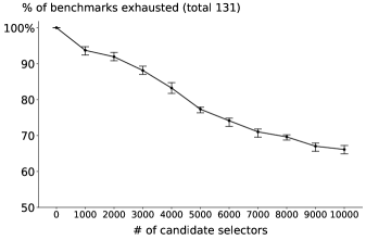
(a) Percentage of exhausted benchmarks vs. number of sampled candidate selectors.

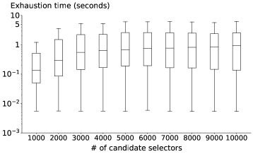
(b) Distribution of exhaustion times against each number of sampled candidate selectors.

Figure 23. RQ3 results. Selectors are sampled uniformly at random from all candidate selectors of size up to four. Arborist exhausts a benchmark’s program space if it terminates before the timeout (i.e., 10 seconds).

Results. Figure 23(a) shows for each $|S|$, how many benchmarks Arborist can successfully exhaust in 10 seconds: since we have multiple runs for each $|S|$, we report the max, median, and min across all runs. Figure 23(b) presents the distribution of exhaustion times — same as in RQ1, we also report quartile statistics here in RQ3 — across all exhausted benchmarks for each $|S|$. The key take-away message is clear: Arborist scales quite well as the number of selectors is increased. For example, with 1,000 candidate selectors, Arborist is able to exhaust the program space for 95% of all 131 benchmarks, with a median exhaustion time of about 0.1 seconds. If we further increase $|S|$ from 1,000 to 5,000, we observe a small drop from 95% to 79% in terms of the percentage of benchmarks that can be exhausted, while the median exhaustion time is under 1 second. Finally, looking at the extreme of 10,000 selectors: 68% benchmarks exhausted with a median of 1-second exhaustion time.

While exhaustion is in general fast, it takes even less time to discover a generalizable program, as also mentioned earlier. For example, among those 68% (i.e., 89) exhausted benchmarks, Arborist can discover an intended program for 61 within 1 second (and 43 under 0.5 seconds). In contrast, WebRobot’s enumeration-based algorithm cannot exhaust more than 10 benchmarks (using the same 10-second timeout), even if fed with only 100 selectors. Furthermore, using 10,000 selectors, WebRobot’s median solving time (i.e., returning an intended program) is 10 seconds. These data points again highlight that Arborist’s underlying search algorithm is highly efficient.

5.4. RQ4: Ablation Studies

Impact of observational equivalence. We consider a variant of Arborist with the OE capability disabled. In other words, this ablation has to enumerate loop bodies (which use loop variables), and does not allow sharing across FTA states that correspond to loop bodies. We evaluate this variant under the RQ1 setup: it solves (i.e., generates an intended program for) 56 benchmarks, among which the median synthesis time is 1 second. In contrast, Arborist solves 123 benchmarks with a median running time of 0.02 seconds across those solved. This again highlights the importance of OE for speeding up the search.

Impact of incremental FTA construction. This ablation builds the FTA $\mathcal{A}$ from scratch given new input traces, without reusing previous FTAs. That is, the incremental FTA construction optimization in Section 4.8 is disabled. We run this ablation using the RQ1 setup. It solves (i.e., returns an intended program for) 105 benchmarks — out of these solved benchmarks, 40 reach the 1-second timeout and the median running time is 0.3 seconds. Arborist solves 18 more benchmarks with only 3 timeouts in total and using a significantly less median time of 0.02 seconds.

5.5. Case Study: Large Language Models

Given the recent advances in large language models (LLMs) and exploding interests in applying them for program synthesis, we conduct a case study where we use LLMs to generate web automation programs from demonstrations. This is mainly a sanity check, and we refer interested readers to the appendix for more details. In summary, our key take-away is that LLMs (in particular, GPT-3.5 (OpenAI, 2022)) fail to generate semantically correct programs, even for some of the simplest benchmarks. The model can produce unstable results, claiming a benchmark is unsolvable in one run while outputting programs in another trial. While these results are poor, it is well-known that LLMs are sensitive to the prompting strategy (Si et al., 2022), and there might be a better method to prompt the model which we have not tried. Nevertheless, we believe these results indicate that our benchmarks are quite hard for state-of-the-art LLMs and require further research in relevant areas in order to better solve these problems.

6. Related Work

In this section, we briefly discuss some closely related work.

Observational equivalence (OE). OE is a very general concept, which states the indistinguishability between multiple entities based on their observed implications. Hennessy and Milner (1980) proposed OE to define the semantics of concurrent programs, where two terms are observationally equivalent whenever they are interchangeable in all observable contexts. The idea of OE has also been adopted by programming-by-example (PBE) (Albarghouthi et al., 2013; Udupa et al., 2013; Peleg et al., 2020) to reduce a large search space of programs thereby boosting the synthesis efficiency. Building upon the concept of OE, our work extends OE-based reduction to also programs with local variables.

Synthesis of programs with local variables. Programs with local variables are evaluated under non-static contexts. To our best knowledge, there are no principled approaches to effectively reduce the space of such programs. Prior work (Wang et al., 2017b; Chen et al., 2021; Feser et al., 2015; Peleg et al., 2020; Chen et al., 2020; Smith and Albarghouthi, 2016) typically falls back to some form of brute-force enumeration or utilizes domain-specific reasoning to prune the search space of programs with local variables (such as lambda bodies). We propose a principled approach — i.e., lifted interpretation — to reduce the space of such programs, thereby speeding up the search of them.

RESL (Peleg et al., 2020) is especially related to our work: it uses an extended context (same as ours) when searching lambdas; however, it does not present a general approach that can reduce such programs. It clearly articulated the key problem of applying OE in general: computing reachable contexts and evaluating programs depend on each other. Our work presents a new algorithm that computes contexts and evaluates programs simultaneously, by constructing the equivalence relation of programs while evaluating programs which facilitates the computation of reachable contexts. In contrast, RESL utilizes rules (manually provided) to infer reachable contexts for lambda bodies, for a given higher-order sketch. For data-dependent functions (like reduce and fold), RESL falls back to enumeration. Our paper addresses the “infeasible hypothesis” from RESL (see D.3 in its appendix). We believe our work also opens up new ways to further study such program synthesis problems.

Lifted Interpretation. Our lifted interpretation idea can be viewed as a bidirectional approach: it traverses the grammar top-down to generate reachable contexts, during which it builds up programs bottom-up given contexts. Different from prior work (Phothilimthana et al., 2016; Gulwani et al., 2011; Lee, 2021) that enumerates programs bidirectionally, we intertwines the enumeration of contexts and programs. Rosette (Torlak and Bodik, 2014) is related, in that they also lift the interpretation from concrete programs to symbolic programs (e.g., defined by a program sketch). A key distinction is that our work directly performs program synthesis and uses finite tree automata to succinctly encode the program space, instead of reducing the search problem to SMT solving.

Finite tree automata (FTAs) for program synthesis. During lifted interpretation, programs are clustered into equivalence classes, succinctly compressed in an FTA. Compared to prior work (Wang et al., 2017b, a, 2018b; Yaghmazadeh et al., 2018; Miltner et al., 2022; Wang et al., 2018a; Handa and Rinard, 2020; Koppel et al., 2022), states in our FTAs encode context-output behaviors, rather than input-output behaviors of programs. The lifted interpretation idea is not tied to FTAs: our algorithm is developed using FTAs, but we believe other data structures (such as VSAs (Gulwani, 2011) or e-graphs (Willsey et al., 2021)), or an enumeration-based approach (Peleg et al., 2020) can also be leveraged.

Program synthesis for web automation. Our instantiation presents a new program synthesis algorithm for web automation. This is an important domain with a long line of work (Chasins et al., 2018; Dong et al., 2022; Pu et al., 2022; Chen et al., 2023; Pu et al., 2023; Barman et al., 2016; Chasins et al., 2015; Leshed et al., 2008; Lin et al., 2009; Fischer et al., 2021; Little et al., 2007) in both human-computer interaction and programming languages. The most related work is WebRobot (Dong et al., 2022): building upon its trace semantics, we further develop a novel synthesis algorithm that can automate a significantly broader range of more challenging tasks much more efficiently.

Programming-by-demonstration (PBD). In particular, our algorithm is a form of programming-by-demonstration that synthesizes programs from a user-demonstrated trace of actions. Different from prior PBD work (Chasins et al., 2018; Dong et al., 2022; Mo, 1990; Lieberman, 1993; Lau et al., 2003) that is based on either brute-force enumeration or heuristic search of programs, Arborist uses observational equivalence to reduce the search space and leverages finite tree automata to succinctly represent all equivalence classes of programs.

7. Conclusion

We proposed lifted interpretation, which is a general approach to reduce the space of programs with local variables, thereby accelerating program synthesis. We illustrated how lifted interpretation works on a simple functional language, and presented a full-fledged instantiation of it to perform programming-by-demonstration for web automation. Evaluation results in the web automation domain show that lifted interpretation allows us to build a synthesizer that significantly outperforms state-of-the-art techniques.

Appendix A Lifted Interpretation Rules for Example in Section 3

$\displaystyle\centering\begin{array}[]{cc}(1)&\mkern-2.0mu\displaystyle\frac{\begin{array}[]{c}\delta=f(q_{1},\cdots,q_{n})\rightarrow q\in\Delta\ \ \ \Gamma\vdash\delta;\Delta\rightsquigarrow(q^{\prime},\Delta^{\prime})\end{array}}{\vphantom{,}\Gamma\vdash q;\Delta\rightsquigarrow(q^{\prime},\Delta^{\prime})}\par\mkern-2.0mu\\ \\ (2)&\mkern-2.0mu\displaystyle\frac{\begin{array}[]{c}\Gamma\vdash q_{1};\Delta\rightsquigarrow(q^{\prime}_{1},\Delta^{\prime}_{1})\ \ \ \ \Gamma\mapsto lst\in\textit{Footprint}(q^{\prime}_{1})\ \ \ \ \Gamma,lst\vdash q_{2};\Delta\rightsquigarrow(q^{\prime}_{2},\Delta^{\prime}_{2})\\ v_{0}=0\ \ \ \ \Gamma\big{[}acc\mapsto v_{i-1},elem\mapsto lst[i]\big{]}\mapsto v_{i}\in\textit{Footprint}(q^{\prime}_{2})\ \ \ \ i\in[1,|lst|]\\ \Omega=\textit{Footprint}(q)\ \ \ \ \Omega^{\prime}=\Omega\cup\{\Gamma\mapsto v_{|lst|}\}\ \ \ \ q^{\prime}=\textit{MkState}(\textsf{P},\Omega^{\prime})\end{array}}{\vphantom{,}\Gamma\vdash\textnormal{fold}(q_{1},q_{2})\rightarrow q;\Delta\rightsquigarrow(q^{\prime},\Delta^{\prime}_{1}\cup\Delta^{\prime}_{2}\cup\{\textnormal{fold}(q^{\prime}_{1},q^{\prime}_{2})\rightarrow q^{\prime}\})}\par\mkern-2.0mu\\ \\ (3)&\mkern-2.0mu\displaystyle\frac{\begin{array}[]{c}v_{0}=0\ \ \ \ q^{\prime}_{0}=q\ \ \ \ \Delta^{\prime}_{0}=\Delta\ \ \ \ i\in[1,|lst|]\\ \Gamma_{i-1}=\Gamma\big{[}acc\mapsto v_{i-1},elem\mapsto lst[i]\big{]}\ \ \ \ \Gamma_{i-1}\vdash q^{\prime}_{i-1};\Delta^{\prime}_{i-1}\rightsquigarrow(q^{\prime}_{i},\Delta^{\prime}_{i})\ \ \ \ \Gamma_{i-1}\mapsto v_{i}\in\textit{Footprint}(q^{\prime}_{i})\end{array}}{\vphantom{,}\Gamma,lst\vdash q;\Delta\rightsquigarrow(q^{\prime}_{|lst|},\Delta^{\prime}_{|lst|})}\par\mkern-2.0mu\\ \\ (4)&\mkern-2.0mu\displaystyle\frac{\Gamma[x]=lst\ \ \ \ \Omega=\textit{Footprint}(q)\ \ \ \ \Omega^{\prime}=\Omega\cup\{\Gamma\mapsto lst\}\ \ \ \ q^{\prime}=\textit{MkState}(\textsf{L},\Omega^{\prime})}{\vphantom{,}\Gamma\vdash x\rightarrow q;\Delta\rightsquigarrow(q^{\prime},\{x\rightarrow q^{\prime}\})}\par\mkern-2.0mu\\ \\ (5)&\mkern-2.0mu\displaystyle\frac{\begin{array}[]{c}\Gamma\vdash q_{1};\Delta\rightsquigarrow(q^{\prime}_{1},\Delta^{\prime}_{1})\ \ \ \ \Gamma\mapsto v_{1}\in\textit{Footprint}(q^{\prime}_{1})\ \ \ \ \Gamma\vdash q_{2};\Delta\rightsquigarrow(q^{\prime}_{2},\Delta^{\prime}_{2})\ \ \ \ \Gamma\mapsto v_{2}\in\textit{Footprint}(q^{\prime}_{2})\\ \Omega=\textit{Footprint}(q)\ \ \ \ \Omega^{\prime}=\Omega\cup\{\Gamma\mapsto v1+v2\}\ \ \ \ q^{\prime}=\textit{MkState}(\textsf{E},\Omega^{\prime})\\ \end{array}}{\vphantom{,}\Gamma\vdash\textnormal{add}(q_{1},q_{2})\rightarrow q;\Delta\rightsquigarrow(q^{\prime},\Delta^{\prime}_{1}\cup\Delta^{\prime}_{2}\cup\{\textnormal{add}(q^{\prime}_{1},q^{\prime}_{2})\rightarrow q^{\prime}\})}\par\mkern-2.0mu\\ \\ (6)&\mkern-2.0mu\displaystyle\frac{\begin{array}[]{c}\Gamma\vdash q_{1};\Delta\rightsquigarrow(q^{\prime}_{1},\Delta^{\prime}_{1})\ \ \ \ \Gamma\mapsto v_{1}\in\textit{Footprint}(q^{\prime}_{1})\ \ \ \ \Gamma\vdash q_{2};\Delta\rightsquigarrow(q^{\prime}_{2},\Delta^{\prime}_{2})\ \ \ \ \Gamma\mapsto v_{2}\in\textit{Footprint}(q^{\prime}_{2})\\ \Omega=\textit{Footprint}(q)\ \ \ \ \Omega^{\prime}=\Omega\cup\{\Gamma\mapsto v1\times v2\}\ \ \ \ q^{\prime}=\textit{MkState}(\textsf{E},\Omega^{\prime})\\ \end{array}}{\vphantom{,}\Gamma\vdash\textnormal{mult}(q_{1},q_{2})\rightarrow q;\Delta\rightsquigarrow(q^{\prime},\Delta^{\prime}_{1}\cup\Delta^{\prime}_{2}\cup\{\textnormal{mult}(q^{\prime}_{1},q^{\prime}_{2})\rightarrow q^{\prime}\})}\par\mkern-2.0mu\\ \\ (7)&\mkern-2.0mu\displaystyle\frac{\Gamma[acc]=v\ \ \ \ \Omega=\textit{Footprint}(q)\ \ \ \ \Omega^{\prime}=\Omega\cup\{\Gamma\mapsto v\}\ \ \ \ q^{\prime}=\textit{MkState}(\textsf{E},\Omega^{\prime})}{\vphantom{,}\Gamma\vdash acc\rightarrow q\rightsquigarrow(q^{\prime},\{acc\rightarrow q^{\prime}\})}\par\mkern-2.0mu\\ \\ (8)&\mkern-2.0mu\displaystyle\frac{\Gamma[elem]=v\ \ \ \ \Omega=\textit{Footprint}(q)\ \ \ \ \Omega^{\prime}=\Omega\cup\{\Gamma\mapsto v\}\ \ \ \ q^{\prime}=\textit{MkState}(\textsf{E},\Omega^{\prime})}{\vphantom{,}\Gamma\vdash elem\rightarrow q\rightsquigarrow(q^{\prime},\{elem\rightarrow q^{\prime}\})}\par\mkern-2.0mu\\ \\ (9)&\mkern-2.0mu\displaystyle\frac{\Omega=\textit{Footprint}(q)\ \ \ \ \Omega^{\prime}=\Omega\cup\{\Gamma\mapsto 1\}\ \ \ \ q^{\prime}=\textit{MkState}(\textsf{E},\Omega^{\prime})}{\vphantom{,}\Gamma\vdash 1\rightarrow q\rightsquigarrow(q^{\prime},\{1\rightarrow q^{\prime}\})}\par\mkern-2.0mu\\ \\ (10)&\mkern-2.0mu\displaystyle\frac{\Omega=\textit{Footprint}(q)\ \ \ \ \Omega^{\prime}=\Omega\cup\{\Gamma\mapsto 2\}\ \ \ \ q^{\prime}=\textit{MkState}(\textsf{E},\Omega^{\prime})}{\vphantom{,}\Gamma\vdash 2\rightarrow q\rightsquigarrow(q^{\prime},\{2\rightarrow q^{\prime}\})}\par\mkern-2.0mu\end{array}\@add@centering$

Figure 24. Lifted interpretation rules for the example from Section 3.

Appendix B Rules for FTA Evaluation in Section 4

$\displaystyle\small\centering\begin{array}[]{cc}(S1)&\mkern-2.0mu\displaystyle\frac{\begin{array}[]{c}q^{\prime}_{0}=q\ \ \ \Delta^{\prime}_{0}=\Delta\ \ \ C_{i}\vdash q^{\prime}_{i-1};\Delta^{\prime}_{i-1}\rightsquigarrow(q^{\prime}_{i},\Delta^{\prime}_{i})\ \ \ i\in[1,n]\end{array}}{\vphantom{,}C_{1},\cdots,C_{n}\vdash q;\Delta\rightsquigarrow(q^{\prime}_{n},\Delta^{\prime}_{n})}\par\mkern-2.0mu\\ \\ (S2)&\mkern-2.0mu\displaystyle\frac{\begin{array}[]{c}\delta=f(q_{1},\cdots,q_{n})\rightarrow q\in\Delta\ \ \ C\vdash\delta;\Delta\rightsquigarrow(q^{\prime},\Delta^{\prime})\end{array}}{\vphantom{,}C\vdash q;\Delta\rightsquigarrow(q^{\prime},\Delta^{\prime})}\par\mkern-2.0mu\\ \\ (S3)&\mkern-2.0mu\displaystyle\frac{\begin{array}[]{c}\Pi=[\pi_{1},\cdots,\pi_{m}]\ \ \ \ \Gamma,\pi_{1}\vdash se:{\raisebox{1.0pt}{$\chi$}}\\ \Omega=\textit{Footprint}(q)\\ \Omega^{\prime}=\Omega\cup\{\Pi,\Gamma\mapsto{\raisebox{1.0pt}{$\chi$}}\}\ \ \ \ q^{\prime}=\textit{MkState}(\textsf{se},\Omega^{\prime})\end{array}}{\vphantom{,}\Pi,\Gamma\vdash se\rightarrow q;\Delta\rightsquigarrow(q^{\prime},\{se\rightarrow q^{\prime}\})}\par\mkern-2.0mu\\ \\ (S4)&\mkern-2.0mu\displaystyle\frac{\begin{array}[]{c}\Gamma\vdash de:L\ \ \ \ \Omega=\textit{Footprint}(q)\\ \Omega^{\prime}=\Omega\cup\{\Pi,\Gamma\mapsto L\}\ \ \ \ q^{\prime}=\textit{MkState}(\textsf{de},\Omega^{\prime})\end{array}}{\vphantom{,}\Pi,\Gamma\vdash de\rightarrow q;\Delta\rightsquigarrow(q^{\prime},\{de\rightarrow q^{\prime}\})}\par\mkern-2.0mu\\ \\ (S5)&\mkern-2.0mu\displaystyle\frac{\begin{array}[]{c}\Pi,\Gamma\vdash q_{1};\Delta\rightsquigarrow(q^{\prime}_{1},\Delta^{\prime}_{1})\ \ \ \ \Pi,\Gamma\mapsto{\raisebox{1.0pt}{$\chi$}}\in\textit{Footprint}(q^{\prime}_{1})\\ \Omega=\textit{Footprint}(q)\ \ \ \ \Pi=[\pi_{1},\cdots,\pi_{m}]\ \ \ \ A^{\prime}=[\emph{Click}({\raisebox{1.0pt}{$\chi$}})]\\ \Omega^{\prime}=\Omega\cup\{\Pi,\Gamma\mapsto A^{\prime},[\pi_{2},\cdots,\pi_{m}]\}\ \ \ \ q^{\prime}=\textit{MkState}(\textsf{E},\Omega^{\prime})\end{array}}{\vphantom{,}\Pi,\Gamma\vdash\emph{Click}(q_{1})\rightarrow q;\Delta\rightsquigarrow(q^{\prime},\Delta^{\prime}_{1}\cup\{\emph{Click}(q^{\prime}_{1})\rightarrow q^{\prime}\})}\par\mkern-2.0mu\\ \\ (S6)&\mkern-2.0mu\displaystyle\frac{\begin{array}[]{c}\Pi,\Gamma\vdash q_{1};\Delta\rightsquigarrow(q^{\prime}_{1},\Delta^{\prime}_{1})\ \ \ \ \Pi,\Gamma\mapsto A^{\prime}_{1},\Pi^{\prime}_{1}\in\textit{Footprint}(q^{\prime}_{1})\\ \Pi^{\prime}_{1},\Gamma\vdash q_{2};\Delta\rightsquigarrow(q^{\prime}_{2},\Delta^{\prime}_{2})\ \ \ \ \Pi^{\prime}_{1},\Gamma\mapsto A^{\prime}_{2},\Pi^{\prime}_{2}\in\textit{Footprint}(q^{\prime}_{2})\\ \Omega=\textit{Footprint}(q)\ \ \ \Omega^{\prime}=\Omega\cup\{\Pi,\Gamma\mapsto A^{\prime}_{1}\mkern 0.0mu\texttt{+}\mkern-1.0mu\texttt{+}\mkern 1.0muA^{\prime}_{2},\Pi^{\prime}_{2}\}\ \ \ q^{\prime}=\textit{MkState}(\textsf{P},\Omega^{\prime})\end{array}}{\vphantom{,}\Pi,\Gamma\vdash\emph{Seq}(q_{1},q_{2})\rightarrow q;\Delta\rightsquigarrow(q^{\prime},\Delta^{\prime}_{1}\cup\Delta^{\prime}_{2}\cup\{\emph{Seq}(q^{\prime}_{1},q^{\prime}_{2})\rightarrow q^{\prime}\})}\par\mkern-2.0mu\\ \\ (S7)&\mkern-2.0mu\displaystyle\frac{\begin{array}[]{c}\Omega=\textit{Footprint}(q)\\ \Omega^{\prime}=\Omega\cup\{\Pi,\Gamma\mapsto\texttt{[]},\Pi\}\\ q^{\prime}=\textit{MkState}(\textsf{P},\Omega)\end{array}}{\vphantom{,}\Pi,\Gamma\vdash\emph{skip}\rightarrow q;\Delta\rightsquigarrow(q^{\prime},\{\emph{skip}\rightarrow q^{\prime}\})}\par\mkern-2.0mu\\ \\ (S8)&\mkern-2.0mu\displaystyle\frac{\begin{array}[]{c}\ \textit{SubFTA}(q,\Delta)=\big{(}\{q\},\Delta^{\prime}\big{)}\\ \end{array}}{\vphantom{,}\texttt{[]},\Gamma\vdash q;\Delta\rightsquigarrow(q,\Delta^{\prime})}\par\mkern-2.0mu\end{array}\@add@centering$

Figure 25. EvaluateFTA rules for loop-free statements in Section 4.

$\displaystyle\small\centering\begin{array}[]{cc}(S9)&\mkern-2.0mu\displaystyle\frac{\begin{array}[]{c}\Pi,\Gamma\vdash q_{1};\Delta\rightsquigarrow(q^{\prime}_{1},\Delta^{\prime}_{1})\ \ \ \ \Pi,\Gamma\mapsto L\in\textit{Footprint}(q^{\prime}_{1})\\ \Pi,\Gamma,L\vdash q_{2};\Delta\rightsquigarrow(q^{\prime}_{2},\Delta^{\prime}_{2})\ \ \ \ \Pi,\Gamma\big{[}z\mapsto L[i]\big{]}\mapsto A^{\prime}_{i},\Pi^{\prime}_{i}\in\textit{Footprint}(q^{\prime}_{2})\ \ \ \ i\in[1,|L|]\\ \Omega=\textit{Footprint}(q)\ \ \ \ \Omega^{\prime}=\Omega\cup\{\Pi,\Gamma\mapsto A^{\prime}_{1}\mkern 0.0mu\texttt{+}\mkern-1.0mu\texttt{+}\mkern 1.0mu\cdots\mkern 0.0mu\texttt{+}\mkern-1.0mu\texttt{+}\mkern 1.0muA^{\prime}_{|L|},\Pi^{\prime}_{|L|}\}\ \ \ \ q^{\prime}=\textit{MkState}(\textsf{P},\Omega^{\prime})\end{array}}{\vphantom{,}\Pi,\Gamma\vdash\emph{ForData}(q_{1},q_{2})\rightarrow q;\Delta\rightsquigarrow(q^{\prime},\Delta^{\prime}_{1}\cup\Delta^{\prime}_{2}\cup\{\emph{ForData}(q^{\prime}_{1},q^{\prime}_{2})\rightarrow q^{\prime}\})}\par\mkern-2.0mu\\ \\ (S10)&\mkern-2.0mu\displaystyle\frac{\begin{array}[]{c}q^{\prime}_{0}=q\ \ \ \ \Delta^{\prime}_{0}=\Delta\ \ \ \ \Pi^{\prime}_{0}=\Pi\\ \Pi^{\prime}_{i-1},\Gamma[z\mapsto v_{i}]\vdash q^{\prime}_{i-1};\Delta^{\prime}_{i-1}\rightsquigarrow(q^{\prime}_{i},\Delta^{\prime}_{i})\ \ \ \ \Pi^{\prime}_{i-1},\Gamma[z\mapsto v_{i}]\mapsto A^{\prime}_{i},\Pi^{\prime}_{i}\in\textit{Footprint}(q^{\prime}_{i})\end{array}}{\vphantom{,}\Pi,\Gamma,[v_{1},\cdots,v_{n}]\vdash q;\Delta\rightsquigarrow(q^{\prime}_{n},\Delta^{\prime}_{n})}\par\mkern-2.0mu\\ \\ (S11)&\mkern-2.0mu\displaystyle\frac{\begin{array}[]{c}\Pi,\Gamma\vdash q_{1};\Delta\rightsquigarrow(q^{\prime}_{1},\Delta^{\prime}_{1})\ \ \ \ \Pi,\Gamma\mapsto se/\psi[i]\in\textit{Footprint}(q^{\prime}_{1})\\ \Pi,\Gamma,se/\psi[i]\vdash q_{2};\Delta\rightsquigarrow(q^{\prime}_{2},\Delta^{\prime}_{2})\ \ \ \ \Pi^{\prime}_{i}=\Pi\\ \Pi^{\prime}_{i+k},\Gamma\big{[}y\mapsto se/\psi[i+k]\big{]}\mapsto A^{\prime}_{i+k},\Pi^{\prime}_{i+k}\in\textit{Footprint}(q^{\prime}_{2})\ \ \ \ k\in[0,l-1]\\ \Pi^{\prime}_{i+l},\Gamma\big{[}y\mapsto se/\psi[i+l]\big{]}\mapsto A^{\prime}_{i+l},\Pi^{\prime}_{i+l}\not\in\textit{Footprint}(q^{\prime}_{2})\\ \Omega=\textit{Footprint}(q)\ \ \ \ \Omega^{\prime}=\Omega\cup\{\Pi,\Gamma\mapsto A^{\prime}_{i}\mkern 0.0mu\texttt{+}\mkern-1.0mu\texttt{+}\mkern 1.0mu\cdots\mkern 0.0mu\texttt{+}\mkern-1.0mu\texttt{+}\mkern 1.0muA^{\prime}_{i+l-1},\Pi^{\prime}_{i+l-1}\}\ \ \ \ q^{\prime}=\textit{MkState}(\textsf{P},\Omega^{\prime})\end{array}}{\vphantom{,}\Pi,\Gamma\vdash\emph{ForSelectors}(q_{1},q_{2})\rightarrow q;\Delta\rightsquigarrow(q^{\prime},\Delta^{\prime}_{1}\cup\Delta^{\prime}_{2}\cup\{\emph{ForSelectors}(q^{\prime}_{1},q^{\prime}_{2})\rightarrow q^{\prime}\})}\par\mkern-2.0mu\\ \\ (S12)&\mkern-2.0mu\displaystyle\frac{\begin{array}[]{c}\Pi,\Gamma\big{[}y\mapsto se[i]\big{]}\vdash q;\Delta\rightsquigarrow(q^{\prime},\Delta^{\prime})\ \ \ \ \Pi,\Gamma\big{[}y\mapsto se[i]\big{]}\mapsto A^{\prime},\Pi^{\prime}\in\textit{Footprint}(q^{\prime})\\ \Pi^{\prime},\Gamma,{\raisebox{1.0pt}{$\chi$}}/\psi[i+1]\vdash q^{\prime};\Delta^{\prime}\rightsquigarrow(q^{\prime},\Delta^{\prime})\par\end{array}}{\vphantom{,}\Pi,\Gamma,se/\psi[i]\vdash q;\Delta\rightsquigarrow(q^{\prime},\Delta^{\prime})}\par\mkern-2.0mu\\ \\ (S13)&\mkern-2.0mu\displaystyle\frac{\textit{SubFTA}(q,\Delta)=(\{q\},\Delta^{\prime})}{\vphantom{,}\texttt{[]},\Gamma,se/\psi[i]\vdash q;\Delta\rightsquigarrow(q,\Delta^{\prime})\par}\par\mkern-2.0mu\\ \\ (S14)&\mkern-2.0mu\displaystyle\frac{\Pi=[\pi_{1},\cdots,\pi_{m}]\ \ \ \ se/\psi[i]\textnormal{ is not a valid selector on }\pi_{1}\ \ \ \ \textit{SubFTA}(q,\Delta)=(\{q\},\Delta^{\prime})}{\vphantom{,}\Pi,\Gamma,se/\psi[i]\vdash q;\Delta\rightsquigarrow(q,\Delta^{\prime})}\par\mkern-2.0mu\\ \\ (S15)&\mkern-2.0mu\displaystyle\frac{\begin{array}[]{c}\texttt{[]},\Pi,\Gamma\vdash(q_{1},q_{2})\rightsquigarrow(q^{\prime}_{1},q^{\prime}_{2},\Delta^{\prime},A^{\prime},\Pi^{\prime})\\ \Omega=\textit{Footprint}(q)\ \ \ \Omega^{\prime}=\Omega\cup\{\Pi,\Gamma\mapsto A^{\prime},\Pi^{\prime}\}\ \ \ q^{\prime}=\textit{MkState}(\textsf{P},\Omega^{\prime})\end{array}}{\vphantom{,}\Pi,\Gamma\vdash\emph{While}(true,q_{1},q_{2})\rightarrow q;\Delta\rightsquigarrow(q^{\prime},\Delta^{\prime}\cup\{\emph{While}(true,q^{\prime}_{1},q^{\prime}_{2})\rightarrow q^{\prime}\})}\par\mkern-2.0mu\\ \\ (S16)&\mkern-2.0mu\displaystyle\frac{\begin{array}[]{c}\Pi,\Gamma\vdash q_{1};\Delta\rightsquigarrow(q^{\prime}_{1},\Delta^{\prime}_{1})\ \ \ \ \Pi,\Gamma\mapsto A^{\prime}_{1},\Pi^{\prime}_{1}\in\textit{Footprint}(q^{\prime}_{1})\\ \Pi^{\prime}_{1},\Gamma\vdash q_{2};\Delta\rightsquigarrow(q^{\prime}_{2},\Delta^{\prime}_{2})\ \ \ \ \Pi^{\prime}_{1},\Gamma\mapsto{\raisebox{1.0pt}{$\chi$}}\in\textit{Footprint}(q^{\prime}_{2})\ \ \ \ A^{\prime}_{2}=[\emph{Click}({\raisebox{1.0pt}{$\chi$}})]\\ \Pi^{\prime}_{1}=[\pi_{1},\pi_{2},\cdots,\pi_{m}]\ \ \ \ \Pi^{\prime}=[\pi_{2},\cdots,\pi_{m}]\ \ \ \ A^{\prime}=A\mkern 0.0mu\texttt{+}\mkern-1.0mu\texttt{+}\mkern 1.0muA^{\prime}_{1}\mkern 0.0mu\texttt{+}\mkern-1.0mu\texttt{+}\mkern 1.0muA^{\prime}_{2}\\ \Delta^{\prime}=\Delta^{\prime}_{1}\cup\Delta^{\prime}_{2}\ \ \ \ A^{\prime},\Pi^{\prime},\Gamma\vdash(q^{\prime}_{1},q^{\prime}_{2});\Delta^{\prime}\rightsquigarrow(q^{\prime\prime}_{1},q^{\prime\prime}_{2},\Delta^{\prime\prime},A^{\prime\prime},\Pi^{\prime\prime})\end{array}}{\vphantom{,}A,\Pi,\Gamma\vdash(q_{1},q_{2});\Delta\rightsquigarrow(q^{\prime\prime}_{1},q^{\prime\prime}_{2},\Delta^{\prime\prime},A^{\prime\prime},\Pi^{\prime\prime})}\par\mkern-2.0mu\\ \\ (S17)&\mkern-2.0mu\displaystyle\frac{}{\vphantom{,}A,\texttt{[]},\Gamma\vdash(q_{1},q_{2});\Delta\rightsquigarrow(q_{1},q_{2},\Delta,A,\texttt{[]})}\par\mkern-2.0mu\\ \\ (S18)&\mkern-2.0mu\displaystyle\frac{\begin{array}[]{c}\Pi,\Gamma\vdash q_{1};\Delta\rightsquigarrow(q^{\prime}_{1},\Delta^{\prime}_{1})\ \ \ \ \Pi,\Gamma\mapsto A^{\prime}_{1},\Pi^{\prime}_{1}\in\textit{Footprint}(q^{\prime}_{1})\\ \Pi^{\prime}_{1}=\texttt{[]}\ \ \ \ \textit{SubFTA}(q_{2},\Delta)=\big{(}\{q_{2}\},\Delta_{2}^{\prime}\big{)}\end{array}}{\vphantom{,}A,\Pi,\Gamma\vdash(q_{1},q_{2});\Delta\rightsquigarrow(q_{1},q_{2},\Delta^{\prime}_{1}\cup\Delta^{\prime}_{2},A\mkern 0.0mu\texttt{+}\mkern-1.0mu\texttt{+}\mkern 1.0muA^{\prime}_{1},\texttt{[]})}\par\mkern-2.0mu\\ \\ (S19)&\mkern-2.0mu\displaystyle\frac{\begin{array}[]{c}\Pi,\Gamma\vdash q_{1};\Delta\rightsquigarrow(q^{\prime}_{1},\Delta^{\prime}_{1})\ \ \ \ \Pi,\Gamma\mapsto A^{\prime}_{1},\Pi^{\prime}_{1}\in\textit{Footprint}(q^{\prime}_{1})\\ \Pi^{\prime}_{1},\Gamma\vdash q_{2};\Delta\rightsquigarrow(q^{\prime}_{2},\Delta^{\prime}_{2})\ \ \ \ \Pi^{\prime}_{1},\Gamma\mapsto{\raisebox{1.0pt}{$\chi$}}\in\textit{Footprint}(q^{\prime}_{2})\\ \Pi^{\prime}_{1}=[\pi_{1},\cdots,\pi_{m}]\ \ \ \ {\raisebox{1.0pt}{$\chi$}}\textnormal{ is not a valid selector on }\pi_{1}\ \ \ \ \textit{SubFTA}(q_{2},\Delta)=\big{(}\{q_{2}\},\Delta_{2}^{\prime}\big{)}\end{array}}{\vphantom{,}A,\Pi,\Gamma\vdash(q_{1},q_{2});\Delta\rightsquigarrow(q_{1},q_{2},\Delta^{\prime}_{1}\cup\Delta^{\prime}_{2},A\mkern 0.0mu\texttt{+}\mkern-1.0mu\texttt{+}\mkern 1.0muA^{\prime}_{1},\Pi^{\prime}_{1})}\par\mkern-2.0mu\end{array}\@add@centering$

Figure 26. EvaluateFTA rules for loopy statements in Section 4.

Appendix C Theorems and Proofs

In this section, we prove the soundness and completeness theorems of our algorithm given a fixed DOM trace $\Pi$ and an action trace $A$.

For simplicity, we use $\emph{Seq}(S_{1},\cdots,S_{k})$ to denote $\emph{Seq}(S_{1},\cdots,\emph{Seq}(S_{k},\emph{skip}))$ and use $\Pi_{[i,j]}$ to denote a slice of the DOM trace $[\pi_{i},\cdots,\pi_{j}]$ (and same for action traces $A$). We also define $P_{1}\mkern 0.0mu\texttt{+}\mkern-1.0mu\texttt{+}\mkern 1.0muP_{2}$, the concatenation of two programs $P_{1}=\emph{Seq}(S_{1},\cdots,S_{k_{1}})$ and $P_{2}=\emph{Seq}(S^{\prime}_{1},\cdots,S^{\prime}_{k_{2}})$, to be $\emph{Seq}(S_{1},\cdots,S_{k_{1}},S^{\prime}_{1},\cdots,S_{k_{2}})$.

C.1. Soundness and completeness of components

In this section, we prove several lemmas about EvaluateFTA and MeregFTAs, which are used in both the soundness theorem and the completeness theorem.

First, we show that the footprints correctly capture the semantics of programs represented by $\mathcal{A}$. To do this, we define a concept called “well-annotatedness”.

Definition C.1.

We call an FTA $\mathcal{A}$ well-annotated if $\mathcal{A}$ satisfies the condition that, for any state $q=(s,\{C_{1}\mapsto O_{1},\cdots,C_{n}\mapsto O_{n}\})$ in $\mathcal{A}$ that represents a program $P$ (that is, $P\in L(\textit{SubFTA}(q,\Delta))$ where $\Delta$ is $\mathcal{A}$’s transitions), we have $C_{i}\vdash P:O_{i}$.

Both EvaluateFTA and MergeFTAs are sound with respect to well-annotatedness; we prove their soundness as lemmas below. These lemmas are later used to establish the soundness of our main algorithm, since they imply $\mathcal{A}$, which is constructed using EvaluateFTA and MergeFTAs, is well-annotated.

Lemma C.2 (Soundness of EvaluateFTA).

Given an unannotated FTA $\mathcal{A}_{s}$ and a list of contexts $[C_{1},\cdots,C_{n}]$, $\textup{{EvaluateFTA}}(\mathcal{A}_{s},[C_{1},\cdots,C_{n}])$ returns a well-annotated FTA.

Proof.

The judgement $C_{1},\cdots,C_{n}\vdash q;\Delta\rightsquigarrow(q^{\prime},\Delta^{\prime})$ “folds” over the judgement over a single context, so we can inductively prove the lemma by inducting on the list $C_{1},\cdots,C_{n}$. The base case holds since any unannotated FTA is a well-annotated FTA. Moreover, it can be proved by induction on the rules that the judgement over a single context, $C\vdash q;\Delta\rightsquigarrow(q^{\prime},\Delta^{\prime})$, only adds footprints consistent with the trace semantics. Therefore, if $(\{q\},\Delta)$ is well-annotated, $(\{q^{\prime}\},\Delta^{\prime})$ is well-annotated as well, which justifies the inductive case. ∎

Lemma C.3 (Soundness and monotonicity of MergeFTAs).

Given two well-annotated FTAs $\mathcal{A}$ and $\mathcal{A}_{e}$ and a state $q$ in $\mathcal{A}$, $\mathcal{A}_{\textit{new}}=\textup{{MergeFTAs}}(\mathcal{A},q,\mathcal{A}_{e})$ is a well-annotated FTA satisfying $L(\mathcal{A})\subseteq L(\mathcal{A}_{\textit{new}})$.

Proof.

Well-annotatedness of $\mathcal{A}_{\textit{new}}$ can be shown by noticing the semantics of MergeFTAs respects the footprints of existing states and the semantics of Seq. We also have $L(\mathcal{A})\subseteq L(\mathcal{A}_{\textit{new}})$ since MergeFTAs only adds new transitions to $\mathcal{A}$. ∎

However, soundness itself does not fully characterize the behavior of EvaluateFTA. For example, both an unannotated FTA and an empty FTA are always well-annotated, but they are not the intended output of EvaluateFTA. Therefore, we additionally prove a completeness theorem of EvaluateFTA, which precisely describes what programs the evaluated FTA should represent and what annotations it should have:

Lemma C.4 (Completeness of EvaluateFTA).

Given an unannotated FTA $\mathcal{A}_{s}$ and a list of contexts $[C_{1},\cdots,C_{n}]$, let $\mathcal{A}_{e}=\textup{{EvaluateFTA}}(\mathcal{A}_{s},[C_{1},\cdots,C_{n}])$. We have $L(\mathcal{A}_{s})=L(\mathcal{A}_{e})$. Moreover, each final state $q\in Q_{f}$ in $\mathcal{A}_{e}$ has contexts $[C_{1},\cdots,C_{n}]$

Proof.

We know that $\mathcal{A}_{e}$ is the union FTA of each $\mathcal{A}^{\prime}_{i}=({q^{\prime}_{i}},\Delta^{\prime}_{i})$ where $C\vdash q_{i};\Delta\rightsquigarrow(q_{i}^{\prime},\Delta^{\prime})$ and $q_{i}$ is a final state of $\mathcal{A}_{s}$. It can be proved that rules over the judgement $C\vdash q_{i};\Delta\rightsquigarrow(q_{i}^{\prime},\Delta^{\prime})$ for a single context $C$ preserves the invariant that $L(\mathcal{A}_{i})=L(\mathcal{A}^{\prime}_{i})$ where $\mathcal{A}_{i}=(\{q_{i}\},\Delta)$. By induction the invariant is also preserved for the judgement over lists of contexts $C_{1},\cdots,C_{n}$, so $L(\mathcal{A})=L(\mathcal{A}_{e})$.

Moreover, it can be shown that $C\vdash q_{i};\Delta\rightsquigarrow(q_{i}^{\prime},\Delta^{\prime})$ maintains the invariant that

$$\textit{GetContexts}(q^{\prime}_{i})=\textit{GetContexts}(q_{i})\cup\{C\}$$

and therefore by induction $C_{1},\cdots,C_{n}\vdash q_{i};\Delta\rightsquigarrow(q_{i}^{\prime},\Delta^{\prime})$ satisfy

$$\textit{GetContexts}(q^{\prime}_{i})=\textit{GetContexts}(q_{i})\cup\{C_{1},\cdots,C_{n}\}$$

which proves the claim as $\mathcal{A}_{s}$ is unannotated. ∎

C.2. Soundness of the synthesis algorithm

Now, we are ready prove the soundness of our main algorithm.

Theorem C.5 (Soundness).

Given input data $I$, input action trace $A$, and input DOM trace $\Pi$, $\mathcal{A}$ contains only programs that reproduce $A$; that is, for all $P\in L(\mathcal{A})$, we have $\Pi_{[1,m]},\Gamma\vdash P:A,\texttt{[]}$, where $\Gamma$ is a binding context with only $x\mapsto I$,

Proof.

We show this by showing that $\mathcal{A}$ is well-annotated, which directly implies the theorem, since the only final state of $\mathcal{A}$ is associated with the footprint $\Pi_{[1,m]},\Gamma\vdash P:A,\texttt{[]}$.

We next prove $\mathcal{A}$ is well-annotated by inducting on the while loop.

• Base case: It is straightforward to see that the initial FTA is well-annotated. For example, consider the set of programs represented by the final state: $\emph{Seq}(a_{1}[\sigma_{1}],\ldots,a_{m}[\sigma_{m}])$ where $\sigma_{i}$ is any substitution that maps full XPaths $\chi$ in $a_{i}$ to selectors $se$ satisfying $\pi_{i},\Gamma\vdash se:{\raisebox{1.0pt}{$\chi$}}$. Any such program $P$ reproduces the trace (i.e., $\Pi_{[1,m]},\Gamma\vdash P:A,[]$).

• Inductive steps: given that $\mathcal{A}$ currently satisfies the invariant, we show that after one iteration of the main loop body (line 9-11 of Algorithm 1), the new $\mathcal{A}$ (denoted as $\mathcal{A}_{\textit{new}}$) still satisfies the invariant. To show this, we notice that by the soundness of EvaluateFTA (Lemma C.4), $\mathcal{A}_{e}$ is well-annotated. Moreover, by the inductive hypothesis, $\mathcal{A}$ is well-annotated as well. According to the soundness of MergeFTAs (Lemma C.3), $\mathcal{A}_{\textit{new}}$ is well-annotated.

∎

C.3. Completeness of the synthesis algorithm

The completeness theorem of our synthesis algorithm is slightly trickier to state Note that our synthesis algorithm does not consider every program that generalizes the trace. For example, our algorithm only synthesizes loops that have two full iterations exhibited in trace. Moreover, our algorithm only consider programs whose generalizability comes from synthesized loops. For example, program $\emph{Seq}(a_{1},\emph{Seq}(a_{1},\emph{skip}))$ generalizes the action trace $[a_{1}]$, but our algorithm does not consider it.

To formally define the program space our synthesis algorithm covers, we introduce a concept called rerollability of an given evaluation. Specifically, we use two judgements to define the set of rerollable programs, $\Pi,\Gamma\vdash^{R}P:A,\Pi^{\prime}\ \textsc{Reroll}$ and $\Pi,\Gamma\vdash^{G}P:A,\Pi^{\prime}\ \textsc{Reroll}$. The only difference between these two judgements is that the first one requires programs to strictly reproduce the trace, and the second one allows the program to also possibly generalize the trace . Specifically, the generalizability judgement allows “skipping evaluations” (similar to the standard semantics of our DSL)

$$(\textsc{Emp-Reroll})\ \ \ \ \ \ \mkern-2.0mu\displaystyle\frac{}{\vphantom{,}\texttt{[]},\Gamma\vdash^{G}P:\texttt{[]},\texttt{[]}\ \textsc{Reroll}}\mkern-2.0mu$$

that the reproducibility judgement does not allow.

Inference rules for rerollability generally follow the semantics of our DSL. However, there are two key differences: First, we require any evaluation of loops must fully reproduce itself in the first two iterations. Second, we track whether a subprogram should strictly reproduce or can potentially generalize the given trace. We show a few representative rules here ($X$ ranges over $\{R,G\}$ in the following rules):

$$\small\begin{array}[]{cc}\\ \\ \textsc{(ForData-Reroll)}&\mkern-2.0mu\displaystyle\frac{\begin{array}[]{c}\Sigma\vdash de:L\ \ \ \ |L|>1\\ \Pi,\Gamma[z\mapsto L[1]]\vdash^{R}P:A_{1},\Pi_{1}\ \textsc{Reroll}\\ \Pi_{1},\Gamma[z\mapsto L[2]]\vdash^{R}P:A_{2},\Pi_{2}\ \textsc{Reroll}\\ \Pi_{i-1},\Gamma[z\mapsto L[i]]\vdash^{X}P:A_{i},\Pi_{i}\ \textsc{Reroll}\ \ \ \ \forall\;i\in[3,|L|]\par\end{array}}{\vphantom{,}\Pi,\Gamma\vdash^{X}\emph{ForData}(de,\lambda z.P):\bigoplus_{i=1}^{|L|}A_{i},\Pi_{|L|}\ \textsc{Reroll}}\par\par\mkern-2.0mu\\ \\ \textsc{(Click-Reroll)}&\mkern-2.0mu\displaystyle\frac{\Pi=[\pi_{1},\cdots,\pi_{m}]\ \ \ \ \pi_{1},\Gamma\vdash se:{\raisebox{1.0pt}{$\chi$}}\ \ \ \ \Pi^{\prime}=[\pi_{2},\cdots,\pi_{m}]}{\vphantom{,}\Pi,\Gamma\vdash^{X}\emph{Click}(se):[{\emph{Click}({\raisebox{1.0pt}{$\chi$}})],\Pi^{\prime}\ \textsc{Reroll}}}\mkern-2.0mu\\ \\ (\textsc{Seq-Non-Final-Reroll})&\mkern-2.0mu\displaystyle\frac{\begin{array}[]{c}P\neq\emph{skip}\\ \Pi,\Gamma\vdash^{R}E:A^{\prime},\Pi^{\prime}\ \textsc{Reroll}\ \ \ \ \Pi^{\prime},\Gamma\vdash^{X}P:A^{{\prime\mkern-2.0mu\prime\mkern-3.0mu}},\Pi^{{\prime\mkern-2.0mu\prime\mkern-3.0mu}}\ \textsc{Reroll}\end{array}}{\vphantom{,}\Pi,\Gamma\vdash^{X}\emph{Seq}(E,P):A^{\prime}\mkern 0.0mu\texttt{+}\mkern-1.0mu\texttt{+}\mkern 1.0muA^{{\prime\mkern-2.0mu\prime\mkern-3.0mu}},\Pi^{{\prime\mkern-2.0mu\prime\mkern-3.0mu}}\ \textsc{Reroll}}\mkern-2.0mu\\ \\ (\textsc{Seq-Final-Reroll})&\mkern-2.0mu\displaystyle\frac{\begin{array}[]{c}\Pi,\Gamma\vdash^{X}E:A^{\prime},\Pi^{\prime}\ \textsc{Reroll}\end{array}}{\vphantom{,}\Pi,\Gamma\vdash^{X}\emph{Seq}(E,\emph{skip}):A^{\prime},\Pi^{\prime}\ \textsc{Reroll}}\par\mkern-2.0mu\end{array}$$

The following lemmas give a sense of the relative restrictiveness of these judgements.

Lemma C.6.

$\Pi,\Gamma\vdash^{R}:A^{\prime},\Pi^{\prime}\ \textsc{Reroll}$ implies $\Pi,\Gamma\vdash^{G}P:A^{\prime},\Pi^{\prime}\ \textsc{Reroll}$.

Lemma C.7.

$\Pi,\Gamma\vdash^{G}:A^{\prime},\Pi^{\prime}\ \textsc{Reroll}$ implies $\Pi,\Gamma\vdash P:A^{\prime},\Pi^{\prime}$.

Proof.

Both lemmas can be proved via a straightforward induction. ∎

Now we have defined the space of rerollable programs we can synthesize, we are ready to show the completeness of our theorem. To prune away programs like $\emph{Seq}(a_{1},\emph{Seq}(a_{1},\emph{skip}))$ for trace $[a_{1}]$, we additionally restrict our completeness theorem to programs whose final expression can produce at least one action on the given trace, as shown below.

Theorem C.8 (Completeness).

Given DOM trace $\Pi$ and environment $\sigma$, if the evaluation of a program $P=\emph{Seq}(S_{1},\cdots,S_{k})$ under $\Pi_{[1,m]}$ and $\Gamma$ is rerollable (and may generalize the given trace) and satisfies that the evaluation of $S_{k}$ produces at least one action, $P$ will be represented by $\mathcal{A}$; In other words, if

$$\Pi_{[1,m]},\Gamma\vdash^{R}\emph{Seq}(S_{1},\cdots,S_{k-1}):A_{[1,p]},\Pi_{[p+1,m]}\ \textup{{Reroll}}$$

and

$$\Pi_{[p+1,m]},\Gamma\vdash^{G}S_{k}:A_{[p+1,m]},\texttt{[]}\ \textup{{Reroll}}$$

where $p\neq m$, then program $\emph{Seq}(S_{1},\cdots,S_{k})\in L(\mathcal{A}).$

Proof.

To prove the theorem, we prove a generalization of it: If

(1) $$\Pi_{[o,m]},\Gamma\vdash^{R}\emph{Seq}(S_{1},\cdots,S_{k-1}):A_{[o,p]},\Pi_{[p+1,m]}\ \textsc{Reroll}$$

and

(2) $$\Pi_{[p+1,m]},\Gamma\vdash^{P}S_{k}:A_{[p+1,q]},\Pi_{[q+1,m]}\ \textsc{Reroll}$$

for some indices $o,p,q$ with $p\neq q$, then

$$\emph{Seq}(S_{1},\cdots,S_{k},a_{j+1},\cdots a_{m})\in L(q_{o},\mathcal{A})$$

for some state $q_{o}$ of $\mathcal{A}$.

We prove this generalization by inducting on the nested levels of loops of program $P$.

• Base case: All loop-free programs $P$ satisfying (1) and (2) have the shape $\emph{Seq}(a_{o}[\sigma_{o}],\cdots,a_{q}[\sigma_{q}])$ where $\sigma_{i}$ is any substitution that maps full XPaths $\chi$ in $a_{i}$ to selectors $se$ satisfying $\pi_{i},\Gamma\vdash se:{\raisebox{1.0pt}{$\chi$}}$. By our construction, there always exists some state $q$ in $\textsc{InitFTA}(\Pi_{[1,m]},A)$ that represents such a program with the corresponding footprints. By the monotonicity of MergeFTAs, this state is in $\mathcal{A}$ and represents such a program as well.

• Inductive steps: Consider a program $P=\emph{Seq}(S_{1},\cdots,S_{k})$ where all $S_{i}$ has a nested level of $n+1$ with rerollable evaluation $\Pi_{[o,m]},\Gamma\vdash^{R}\emph{Seq}(S_{1},\cdots,S_{k_{1}}):A_{[o,p]},\Pi_{[p+1,m]}\ \textsc{Reroll}$ and $\Pi_{[p,m]},\Gamma\vdash^{G}S_{k}:A_{[p,q]},\Pi_{[q+1,m]}\ \textsc{Reroll}$. Let us only consider the case for ForData and other loop forms can be proved similarly.

  To show this statement about $\emph{Seq}(S_{1},\cdots,S_{k})$, we only need to show it for a single $S$. Suppose that $S=\emph{ForData}(de,\lambda z.P^{\prime})$ is an expression from $S_{1},\cdots,S_{k}$ and that $P^{\prime}$ has the form $\emph{Seq}(S^{\prime}_{1},\ldots,S^{\prime}_{l})$ and a nested level of $n$. We will show that if $\Pi_{[i,m]},\Gamma\vdash^{G}S:A_{[i,l]},\Pi_{[l+1,m]}$, then $\emph{Seq}(S,a_{l+1},\cdots,a_{m})\in L(q,\mathcal{A})$ for some $q$.

  By ForData-Reroll, we have

  $$\begin{array}[]{c}\Pi_{[i,m]},\Gamma[z\mapsto L[1]]\vdash^{R}P^{\prime}:A_{[i,j]},\Pi_{[j+1,m]}\ \textsc{Reroll}\\ \Pi_{[j+1,m]},\Gamma[z\mapsto L[2]]\vdash^{R}P^{\prime}:A_{[j+1,k]},\Pi_{[k+1,m]}\ \textsc{Reroll}\end{array}$$

  for some $j,k$. Alternatively, we can apply the substitution with $z$ to $P^{\prime}$ directly.

  $$\begin{array}[]{c}\Pi_{[i,m]},\Gamma\vdash^{R}P^{\prime}[z\mapsto L[1]]:A_{[i,j]},\Pi_{[j+1,m]}\ \textsc{Reroll}\\ \Pi_{[j+1,m]},\Gamma\vdash^{R}P^{\prime}[z\mapsto L[2]]:A_{[j+1,k]},\Pi_{[k+1,m]}\ \textsc{Reroll}\end{array}$$

  It can be proved via a straightforward induction that $P^{\prime}_{\mkern 0.0mu\texttt{+}\mkern-1.0mu\texttt{+}\mkern 1.0mu}=P^{\prime}[z\mapsto L[1]]\mkern 0.0mu\texttt{+}\mkern-1.0mu\texttt{+}\mkern 1.0muP^{\prime}[z\mapsto L[2]]$ satisfy

  $$\Pi_{[i,m]},\Gamma\vdash^{R}P^{\prime}_{\mkern 0.0mu\texttt{+}\mkern-1.0mu\texttt{+}\mkern 1.0mu}:A_{[i,k]},\Pi_{[k+1,m]}\ \textsc{Reroll}.$$

  Moreover, $P^{\prime}_{\mkern 0.0mu\texttt{+}\mkern-1.0mu\texttt{+}\mkern 1.0mu}$ has a nested level of $n$, so by Lemma C.6 and inductive hypothesis, it follows

  $$P^{\prime}_{\mkern 0.0mu\texttt{+}\mkern-1.0mu\texttt{+}\mkern 1.0mu}\mkern 0.0mu\texttt{+}\mkern-1.0mu\texttt{+}\mkern 1.0mu\emph{Seq}(a_{k+1},\cdots,a_{m})\in L(q_{i},\mathcal{A})$$

  for some state $q_{0}$. Expanding the definition of $P^{\prime}_{\mkern 0.0mu\texttt{+}\mkern-1.0mu\texttt{+}\mkern 1.0mu}$:

  $$\begin{array}[]{rr}\emph{Seq}(S^{\prime}_{1}[z\mapsto L[1]],\ldots,S^{\prime}_{k}[z\mapsto L[1]],&\\ S^{\prime}_{1}[z\mapsto L[2]],\ldots,S^{\prime}_{k}[z\mapsto L[2]],&\\ a_{k+1},\cdots,a_{m})&\in L(q_{0},\mathcal{A}).\end{array}$$

  We just show that there will be two consecutive traces of the loop in the FTA, so the matching procedure (line 7 of algorithm 1) will eventually match the root state $q_{0}$ and a list of states $q^{\prime}_{1},\cdots,q^{\prime}_{2l}$ where

  1. $q_{0}=(P,\{\Pi_{[i,m]},\Gamma\mapsto A_{[i,m]},\texttt{[]}\})$,

  2. $S^{\prime}_{i}[z\mapsto L[1]]\in L(q^{\prime}_{i},\mathcal{A})$, and

  3. $S^{\prime}_{i}[z\mapsto L[2]]\in L(q^{\prime}_{l+i},\mathcal{A})$.

  During SpeculateFTA, anti-unifying any pair $q^{\prime}_{i},q^{\prime}_{l+i}$ will yield an anti-unifier $de$ with $\Gamma\vdash de:L$, because per the construction in InitFTA, all states containing $L[1]$ (resp. $L[2]$) will also contain all alternative data expressions $de[1]$ (resp. $de[2]$). As a result, the FTA after speculation, $\mathcal{A}_{s}$, will represent the program $\emph{ForData}(de,\lambda z.\emph{Seq}(S^{\prime}_{1},\cdots,S^{\prime}_{k}))$. This is exactly the $S$ we want to synthesize.

  Finally, by completeness of EvaluateFTA, $S$ is represented by a final state $q$ in $\mathcal{A}_{e}$ as well and $q$ has context $\{P,\Pi_{[i,m]}\}$. By soundness of EvaluateFTA, $\mathcal{A}_{e}$ is well-annotated, so the footprint follows the evaluation and has to be $\{\Pi_{[i,m]},\Gamma\mapsto A_{[i,l]}\}$ for some index $l$ that marks the end of loop evaluation (or the end of the trace) satisfying $\Pi_{[i,m]},\Gamma\vdash S:A_{[i,l]},\Pi_{[l+1,m]}$.

  On the other hand, according to InitFTA, there exists a state $q^{\prime}$ in $\mathcal{A}$ that represents program $\emph{Seq}(a_{l+1},\cdots,a_{m})$ with footprint $\Pi_{[l+1,m]},\Gamma\mapsto A_{[l+1,m]},\texttt{[]}$. Because the root state $q_{0}$ has footprint $\Pi_{[i,m]},\Gamma\mapsto A_{[i,m]},\texttt{[]}$. By definition MergeFTAs will add a transition $\emph{Seq}(q,q^{\prime})\rightarrow q_{0}$ to $\mathcal{A}$, so $q_{0}$ now represents $\emph{Seq}(S,a_{l+1},\cdots,a_{m})$.

∎

C.4. The main theorem

Combining everything together, we have the following main theorem:

Theorem 4.5 0.

Given action trace $A$, DOM trace $\Pi$ and input data $I$, our synthesis algorithm always terminates. Moreover, if there exists a program in our grammar (shown in Figure 8) that generalizes $A$ (given $\Pi$ and $I$) and satisfies the condition that (1) every loop has at least two iterations exhibited in $A$ and (2) its final expression is a loop, then our synthesis algorithm (shown in Algorithm 1) would return a program that generalizes $A$ (given $\Pi$ and $I$) upon FTA saturation.

Proof.

Our algorithm always terminates since there are only finitely many ways to reroll a trace. Moreover, if there exists a program $P$ that generalizes $A$ and satisfies condition (1) and (2), such a program also reproduces $A$ and its last loop expression produces at least one action (since any loop expression has at least two exhibited iterations). By completeness (theorem C.8) of our algorithm, $P$ is represented by $\mathcal{A}$. As a result, the set of generalizing programs is not empty, and Rank will heuristically pick such a program with smallest size. By soundness (theorem C.5) of our algorithm, the returned program is always correct with respect to the given $\Pi$ and $I$. ∎

Appendix D Case Study: Large Language Models

Given the recent advances in large language models (LLMs) and exploding interests in applying them for program synthesis, we perform a case study where we use LLMs to solve program synthesis problems in our domain of web automation.

Setup. Given a benchmark (consisting of an action trace $A$ together with candidate selectors for each action in $A$), we construct a prompt that contains (i) an English description of our web automation language’s syntax and semantics, (ii) a brief explanation of the web automation program synthesis problem (i.e., reproduce the demonstration) together with a small example, and (iii) the input action trace $A$ — including candidate selectors — that we aim to synthesize a program for. Here, (i) and (ii) are shared across benchmarks while (iii) is created in a per-benchmark manner. Once constructed, the prompt is fed to the model which is then queried for 3 completions. We define a benchmark as “solved” if any of the completions gives an intended program. We conduct this evaluation using the GPT-3.5 API (OpenAI, 2022), which is one of the most popular LLMs publicly available nowadays.

A unique technical challenge in our domain is that, we have a large number of candidate selectors as part of the problem specification — as shown in RQ2, it is necessary to consider multiple hundreds of them in order to solve a decent number of benchmarks. The GPT-3.5 model we use, however, supports (only) up to 16,385 tokens, which unfortunately is not large enough to hold all necessary selectors for most of our benchmarks. Therefore, in this experiment, we use a very small subset of our language that contains only ForSelectors loops (with loop index starting at 1) and primitive expressions (like Click). We further focus on benchmarks that can be solved using absolute selectors. This leads us to a total of 14 benchmarks, where the complexity of intended programs ranges from trivial 1-level loops with two expressions to a nested loop with 10 expressions. We truncate the input action trace to include at most 200 actions to fit within the model’s context window. We also make sure this max length is sufficient to generate all intended programs for our 14 benchmarks.

Results. While the model oftentimes generates syntactically reasonable programs (which is quite impressive), it fails to generate semantically correct programs for 7 (out of 14) benchmarks. The 7 successfully solved cases all involve single-level loops with a maximum of 6 statements — these are the simplest benchmarks in our suite. Among the 7 unsolved benchmarks, the model frequently fails to parametrize expressions in the loop body and struggles with constructing desired loop structures. The model sometimes produces unstable results, claiming that a benchmark is unsolvable in one run while outputing programs in the other two trials.

While these results are clearly poor, it is well-known that LLMs are sensitive to the prompting strategy (Si et al., 2022) and there might be a better method to prompt the model. Nevertheless, we believe these results demonstrate that our benchmarks are quite hard for state-of-the-art LLMs and require further research in relevant areas in order to better solve these problems.