Accelerating the Galerkin Reduced-Order Model with the Tensor Decomposition for Turbulent Flows

Abstract

Galerkin-based reduced-order models (G-ROMs) have provided efficient and accurate approximations of laminar flows. In order to capture the complex dynamics of the turbulent flows, standard G-ROMs require a relatively large number of reduced basis functions (on the order of hundreds and even thousands). Although the resulting G-ROM is still relatively low-dimensional compared to the full-order model (FOM), its computational cost becomes prohibitive due to the 3rd-order convection tensor contraction. The 3rd-order tensor requires storage of $N^{3}$ entries with a corresponding work of $2N^{3}$ operations per timestep, which makes such ROMs impossible to use in realistic applications, such as control of turbulent flows. In this paper, we focus on the scenario where the G-ROM requires large $N$ values and propose a novel approach that utilizes the CANDECOMC/PARAFAC decomposition (CPD), a tensor decomposition technique, to accelerate the G-ROM by approximating the 3rd-order convection tensor by a sum of $R$ rank-1 tensors. In addition, we show that the convection tensor is partially skew-symmetric and derive two conditions for the CP decomposition for preserving the skew-symmetry. Moreover, we investigate the G-ROM with the singular value decomposition (SVD). The G-ROM with CP decomposition is investigated in several flow configurations from 2D periodic flow to 3D turbulent flows. Our numerical investigation shows CPD-ROM achieves at least a factor of 10 speedup. Additionally, the skew-symmetry preserving CPD-ROM is more stable and allows the usage of smaller rank $R$. Moreover, from the singular value behavior, the advection tensor formed using the $H^{1}_{0}$-POD basis has a low-rank structure, and this low-rank structure is preserved even in higher Reynolds numbers. Furthermore, for a given level of accuracy, the CP decomposition is more efficient in size and cost than the SVD.

1 Introduction

Reduced order models (ROMs) are computational models that leverage data to approximate the dynamics in a space whose dimension, $N$, is orders of magnitude lower than the dimension of full order models (FOMs), that is models obtained from classical numerical discretizations (e.g., the finite element or spectral element methods). In the numerical simulation of fluid flows, Galerkin ROMs (G-ROMs), which use a data-driven basis in a Galerkin framework, have provided efficient and accurate approximations of laminar flows, such as the two-dimensional flow past a circular cylinder at low Reynolds numbers [9, 36, 60, 67].

For nonlinear problems, due to the nonlinear operators or nonaffine paramter dependence, ROMs are no longer efficient because the evaluation of the nonlinear term depends on the FOM degress of freedoms. Existing techniques for addressing the nonlinear evaluation cost in the ROMs include the EIM [6], the discrete empirical interpolation method (DEIM) [13, 12, 14], the missing point estimation [3], and the gappy POD [10]. These ‘hyper-reduction’ techniques can effectively evaluate nonlinear terms and enable application of pMOR to nonlinear problems.

Although the advection operator in the Navier-Stokes equations (NSE) is nonlinear, it is only of polynomial type. Hence the evaluation cost of the nonlinear term is already indepedent to the FOM degress of freedoms. In fact, a 3rd-order advection tensor can be precomputed in the offline and in the online, the evaluation of the nonlinear term can be done by a tensor contraction with $2N^{3}$ operations per timestep.

However, turbulent flows (e.g., the turbulent channel flow [46, 59]) are notoriously hard for the standard G-ROM. To capture the complex dynamics of the turbulent flow, standard ROMs require a relatively large number (on the order of hundreds and even thousands [1, Table II]) of reduced basis functions to achieve good accuracy. Although the resulting G-ROM is still relatively low-dimensional compared to the FOM, its computational cost becomes prohibitive due to the 3rd-order convection tensor contraction cost $\mathcal{O}(N^{3})$. The 3rd-order tensor requires storage of $N^{3}$ entries with a corresponding work of $2N^{3}$ operations per timestep. While $N=100$, with a cost of a two million operations per step and a million words in memory, may be tolerable, $N=400$ with a cost of $128$ million operations and $64$ million words quickly makes ROMs inefficient. Hence, it is impossible to use such ROMs in realistic applications, such as control of turbulent flows. Hyper-reduction techniques such as DEIM has been applied to the nonlinear term in the steady NSE and the NSE to reduce the computational cost in [77, 24].

In this work, we focus on the scenario where G-ROM requires large $N$ values and investigate the potential of the tensor decomposition for reducing the tensor contraction cost. Tensor decomposition has been widely used as a low-rank approximation for reducing the cost in the FOM level. For example, in [21], low-rank tensor decomposition algorithm has developed for the numerical solution of a distributed optimal control problem constrained by the two-dimensional time-dependent Navier-Stokes equation with a stochastic inflow. Other decomposition such as the hierarchical Tucker decomposition and the tensor train have also been applied to other types of equations, such as the Vlasov equation [31, 23], the Fokker–Planck equation [71], and the Boltzmann equation [15]. Dynamical low-rank approximation has been used to compute low-rank approximations to time-dependent large data matrices or to solutions of large matrix differential equations [47, 62].

In the context of reduced order modeling, tensor decomposition has only been used for extracting multiple space–time basis vectors from each training simulation via tensor decomposition [16]. In [68], the author considered the windowed space-time least-squares Petrov-Galerkin method (WST-LSPG) for model reduction of nonlinear parameterized dynamical systems and proposes constructing space-time bases using tensor decompositions for each window.

In this paper, we propose a novel approach which utilizes the CANDECOMC/PARAFAC decomposition (CPD), a tensor decomposition technique, to accelerate the G-ROM by approximating the ROM advection tensor by a sum of $R$ rank-1 tensors. In addition, we show the ROM advection tensor is partially skew-symmetric and demonstrate there is an underlying CP structure. Moreover, we derive two conditions for the CP decomposition for preserving the skew-symmetry. We found preserving the skew-symmetry provide stability but does not, in general, improve accuracy. This observation is consistent with the behavior of full-order models, which is known as dealiasing. We also investigate the G-ROM with the singular value decomposition (SVD), and found the advection tensor formed using the $H^{1}_{0}$-POD basis has low-rank structure and this low-rank structure is preserved even in higher Reynolds numbers. Additionally, we demonstrated that, for a given level of accuracy, the CP decomposition is more efficient in size and cost than the SVD. The CPD-ROM is investigated in several flow configurations from 2D periodic flow to 3D turublent flows.

The rest of the paper is organized as follows: In Section 2, we provide the backgrounds for the full-order model (FOM), the Galerkin reduced-order model (G-ROM) and the CANDECOMC/PARAFAC decomposition (CPD) for general and partially symmetric tensor. In Section 3, we present the G-ROM with the CP decomposition (CPD-ROM). In Section 4, we present the numerical results. Finally, in Section 5, we present the conclusions of our numerical investigation.

2 Background

In this section, we provide necessary background for the paper. In Section 2.1, we briefly introduce the full-order model (FOM) and suggest [75] for a detail review of the FOM. In Section 2.2, we present the the Galerkin reduced-order model (G-ROM). In Sections 2.3-2.4, we introduce the CANDECOMC/PARAFAC decomposition (CPD) with alternating least squares method (ALS) for general and partially symmetric tensors.

2.1 Full-order model (FOM)

The governing equations are the incompressible Navier-Stokes equations (NSE):

$$\frac{\partial{\bm{u}}}{\partial t}+({\bm{u}}\cdot\nabla){\bm{u}}=-\nabla p+\frac{1}{\rm Re}\nabla^{2}{\bm{u}},\quad\nabla\cdot{\bm{u}}=0.$$ (2.1)

Here ${\bm{u}}$ is the velocity subject appropriate Dirichlet or Neumann boundary conditions, $p$ is the pressure, and $\rm Re$ is the Reynolds number.

We employ the spectral element method (SEM) for the spatial discretization of (2.1). The $P_{q}$–$P_{q-2}$ velocity-pressure coupling [57] is considered where the velocity ${\bm{u}}$ is represented as a tensor-product Lagrange polynomial of degree $q$ in the reference element ${\hat{\Omega}}:=[-1,1]^{2}$ while the pressure $p$ is of degree $q-2$, resulting a velocity space ${\bf X}^{{\cal N}}$ for approximating the velocity and a pressure space $Y^{\bar{{\cal N}}}$ for approximating the pressure, where the finite dimensions ${\cal N}$ and $\bar{{\cal N}}$ are the global numbers of spectral element degress of freedom in the corresponding spectral element spaces.

The semi-discrete weak form of (2.1) reads: Find $({\overline{\bf u}},~{}p)\in({\bf X}^{{\cal N}},Y^{\bar{{\cal N}}})$ such that, for all $({\bm{v}},~{}q)\in({\bf X}^{{\cal N}}_{0},Y^{\bar{{\cal N}}}_{0})$,

$$\left({\bm{v}},\frac{\partial{\overline{\bf u}}}{\partial t}\right)+\biggl{(}({\overline{\bf u}}\cdot\nabla){\overline{\bf u}},{\bm{v}}\biggr{)} =\left(\nabla\cdot{\bm{v}},p\right)-\frac{1}{\rm Re}\,(\nabla{\bm{v}},\nabla{\overline{\bf u}}),$$ (2.2)

$$-\left(q,\nabla\cdot{\overline{\bf u}}\right) =0,$$ (2.3)

where $(\cdot,\cdot)$ denotes as the $L^{2}$ inner product. The diffusive and the pressure terms have different signs due to the application of integration by parts and the divergence theorem.

Following [28], a semi-implicit scheme BDF$k$/EXT$k$ is used for time discretization. The fully discretization leads to a linear unsteady Stokes system. The detailed derivation of the FOM is referred to [75].

2.2 Galerkin reduced-order model (G-ROM)

To construct the G-ROM, we first follow the standard proper orthogonal decomposition (POD) procedure [8, 76] to construct the reduced basis. To this end, we collect a set of velocity snapshots $\{{\bm{u}}^{k}:={\bm{u}}({\bf x},t^{k})-\bm{\varphi}_{0}\}^{K}_{k=1}$, corresponding to the FOM solutions at well-separated timepoints $t^{k}$, minus the zeroth mode $\bm{\varphi}_{0}$ and form its corresponding Gramian matrix using $L^{2}/H^{1}_{0}$ inner product. The first $N$ POD basis $\{\bm{\varphi}_{i}\}^{N}_{i=1}$ are constructed from the first $N$ eigenmodes of the Gramian. Setting the zeroth mode, $\bm{\varphi}_{0}$, to the time-averaged velocity field in the time interval in which the snapshots were collected, the G-ROM is constructed by inserting the ROM basis expansion

$${\bm{u}}_{\text{r}}({\bf x})=\bm{\varphi}_{0}({\bf x})+\sum_{j=1}^{N}u_{\text{r},j}\bm{\varphi}_{j}({\bf x})$$ (2.4)

into the weak form of Equation 2.1: Find ${\bm{u}}_{\text{r}}$ such that, for all ${\bm{v}}\in{\bf X}^{N}_{0}$,

$$\left({\bm{v}}_{i},\frac{\partial{\bm{u}}_{\text{r}}}{\partial t}\right)+\frac{1}{\rm Re}\,\left(\nabla{\bm{v}}_{i},\nabla{\bm{u}}_{\text{r}}\right)+\biggl{(}{\bm{v}}_{i},({\bm{u}}_{\text{r}}\cdot\nabla){\bm{u}}_{\text{r}}\biggr{)}=0,$$ (2.5)

where ${\bf X}^{N}_{0}:=\text{span}\{\bm{\varphi}_{i}\}^{N}_{i=1}$ is the ROM space.

Remark 2.1.

We note that, in the case of fixed geometries, the divergence and pressure terms drop out of (2.5) since the ROM basis is weakly divergence-free. For ROMs that include the pressure approximation, see, e.g., [36, 67, 5, 19, 61].

With (2.5), a system of differential equations in the coefficients with respect to the POD bases $u_{\text{r},j}$ are derived:

$$B\frac{d{\underline{u}}_{\text{r}}}{dt} =-\mathcal{C}(\bar{{\underline{u}}}_{\text{r}})\bar{{\underline{u}}}_{\text{r}}-\frac{1}{\rm Re}A\bar{{\underline{u}}}_{\text{r}},$$ (2.6)

where ${\underline{u}}_{\text{r}}\in\mathbb{R}^{N}$ is the vector consists of POD coefficients $\{u_{r,j}\}^{N}_{j=1}$ and $\bar{{\underline{u}}}_{\text{r}}\in\mathbb{R}^{N+1}$ is the augmented vector that includes the zeroth mode’s coefficient. $A$, $B$, and $\mathcal{C}$ represent the reduced stiffness, mass, and advection operators, respectively, with entries

$$A_{ij}=\int_{\Omega}\nabla\bm{\varphi}_{i}:\nabla\bm{\varphi}_{j}\,dV,\quad B_{ij}=\int_{\Omega}\bm{\varphi}_{i}\cdot\bm{\varphi}_{j}\,dV,\quad\mathcal{C}_{ikj}=\int_{\Omega}\bm{\varphi}_{i}\cdot(\bm{\varphi}_{k}\cdot\nabla)\bm{\varphi}_{j}\,dV.$$ (2.7)

For temporal discretization of (2.6), a semi-implicit scheme with $k$th-order backward differencing (BDF$k$) and $k$th-order extrapolation (EXT$k$) is considered. The fully discretized reduced system at time $t^{l}$ is

$$\left(\frac{\beta_{0}}{\Delta t}B+\frac{1}{\rm Re}A\right)\,{\underline{u}}_{\text{r}}^{l+1} =-\sum^{k}_{i=1}\alpha_{i}\left[\mathcal{C}({{\underline{u}}}^{l-i}){{\underline{u}}}^{l-i}+(C_{1}+C_{2})\bar{{\underline{u}}}^{l-i}-\underline{c}_{0}\right]-B\sum^{k}_{i=1}\frac{\beta_{i}}{\Delta t}{\underline{u}}^{l-i}-\frac{1}{\rm Re}\underline{a}_{0},$$ (2.8)

where

$$c_{0,i} =\int_{\Omega}\bm{\varphi}_{i}\cdot(\bm{\varphi}_{0}\cdot\nabla)\bm{\varphi}_{0}\,dV,\quad a_{0,i}=\int_{\Omega}\nabla\bm{\varphi}_{i}:\nabla\bm{\varphi}_{0}\,dV,$$ (2.9)

$$C_{1,ij} =\int_{\Omega}\bm{\varphi}_{i}\cdot(\bm{\varphi}_{0}\cdot\nabla)\bm{\varphi}_{j}\,dV,\quad C_{2,ik}=\int_{\Omega}\bm{\varphi}_{i}\cdot(\bm{\varphi}_{k}\cdot\nabla)\bm{\varphi}_{0}\,dV,$$ (2.10)

for all $i=1,\ldots,N$ and $j,~{}k=0,\ldots,N$.

Remark 2.2.

The computational cost of solving (2.8) is dominated by the application of the rank-3 advection tensors, $\mathcal{C}$, which requires $O(N^{3})$ operations and memory references on each step. The remainder of the terms are $O(N^{2})$ or less. Unfortunately, $O(N^{3})$ is a very steep cost and prohibits practical consideration of, say, $N>200$. In this paper, our goal is to mitigate the cost with CP decomposition.

2.3 CP decomposition with ALS

The CP decomposition [34, 38] factorizes a tensor into a sum of component rank-one tensors. For example, given a third-order tensor $\mathcal{X}\in\mathbb{R}^{s_{1}\times s_{2}\times s_{3}}$, its CP decomposition is denoted by

$$\mathcal{X}\approx\llbracket A^{(1)},A^{(2)},A^{(3)}\rrbracket\equiv\sum^{R}_{r=1}{\underline{a}}^{(1)}_{r}\circ{\underline{a}}^{(2)}_{r}\circ{\underline{a}}^{(3)}_{r}.$$ (2.11)

where $\llbracket~{}\rrbracket$ is the Kruskal operator [50] which provides shorthand notation for the sum of the outer products of the columns of a set of matrices. $A^{(i)}=\left[{\underline{a}}^{(i)}_{1},\cdots,{\underline{a}}^{(i)}_{R}\right]\in\mathbb{R}^{s_{i}\times R}$ for $i=1,2,3$ are the factor matrices and refer to the combination of the vectors from the rank-one components and $R$ is the CP rank. It is noteworthy to point out that solving Equation 2.11 with $R=1$ is already NP-hard [37].

The rank of a tensor $\mathcal{X}$ is defined as the smallest number of rank-one tensors that generate $\mathcal{X}$ as their sum [38, 52]. One of the major differences between matrix and tensor rank [49] is that determining the rank of a specific tensor is NP-hard [35]. Consequently, the first issue that arises in computing a CP decomposition is how to choose the number of rank-one components. In this paper, we consider the most common strategy by simply fitting multiple CP decompositions with different $R$ until one is ”good”.

For a given CP rank $R$, finding a CP decomposition for $\mathcal{X}$ corresponds to a nonlinear least-squares optimization problem:

$$\min_{A^{(1)},A^{(2)},A^{(3)}}\|\mathcal{X}-\llbracket A^{(1)},A^{(2)},A^{(3)}\rrbracket\|_{F},$$ (2.12)

where $\|\cdot\|_{F}$ is the Frobenius norm and the Frobenius norm of a tensor $\mathcal{X}\in\mathbb{R}^{s_{1}\times s_{2}\times s_{3}}$ is the square root of the sum of the squares of all its elements.

There are many algorithms to compute CP decomposition. In this paper, we consider the alternating least squares (ALS) method [11, 34]. The idea behind ALS is that we solve for each factor in turn, leaving all the other factor fixed. In each iteration, three subproblems are solved in sequence:

$$\min_{B\in\mathbb{R}^{s_{1}\times R}}\|\mathcal{X}-\llbracket B,A^{(2)},A^{(3)}\rrbracket\|_{F},~{}\min_{B\in\mathbb{R}^{s_{2}\times R}}\|\mathcal{X}-\llbracket A^{(1)},B,A^{(3)}\rrbracket\|_{F},~{}\min_{B\in\mathbb{R}^{s_{3}\times R}}\|\mathcal{X}-\llbracket A^{(1)},A^{(2)},B\rrbracket\|_{F}.$$ (2.13)

Each subproblem corresponds to a linear least squares problem and is often solved via the normal equation [49], which involves tensor contraction to solve the linear system of equation and costs $\mathcal{O}(s^{3}R)$ if $s_{i}=s$ for all $i\in\{1,2,3\}$.

2.4 CP decomposition for partially symmetric tensor

Symmetric tensor plays an important role in many fields, for example, chemometrics, psychometrics, econometrics, image processing, biomedical signal processing, etc [18, 66, 17, 43]. A tensor is symmetric if its elements remain the same under any permutation of the indices [49]. Tensors can be partially symmetric in two or more modes as well.

The CP decomposition for partially symmetric tensor has been studied in [11, 48]. Assume the tensor $\mathcal{X}$ is symmetric in the mode-$1$ and mode-$3$, its CP decomposition is symmetric if:

$$\mathcal{X}\approx\llbracket A^{(1)},A^{(2)},A^{(3)}\rrbracket=\llbracket A^{(3)},A^{(2)},A^{(1)}\rrbracket.$$ (2.14)

Typically, one can ensure Equation 2.14 by enforcing the factor matrix $A^{(1)}$ and $A^{(3)}$ to be the same. For fully symmetric tensors, setting $A^{(1)}=A^{(2)}=A^{(3)}$ results in a decomposition whose rank is referred to as the symmetric rank of a tensor. For such tensors, the symmetric rank is often the same as the CP rank [17].

The factor $A^{(2)}$ is computed as in ALS. For $A^{(1)}$ and $A^{(3)}$, we use an iterative algorithm [39] similar to the Babylonian square root algorithm, which updates $A^{(1)}$ using a series of subiterations. At each subiteration, a linear least squares problem is solved for one of the two repeated factors (with the other fixed),

$$A^{(1)}_{\text{next}}=\underset{B}{\mathrm{argmin}}\|\mathcal{X}-\llbracket B,A^{(2)},A^{(1)}\rrbracket\|.$$ (2.15)

Then both the first and third factors are updated with momentum, $A^{(1)}_{\text{new}}=\lambda A^{(1)}+(1-\lambda)A^{(1)}_{\text{next}}$.

3 Accelerating the G-ROM with CP decomposition

The motivation to consider CP decomposition for the G-ROM is demonstrated in Fig. 3.1. Fig. 1(a) shows the behavior of the accumulated POD eigenvalue for 2D periodic to 3D turbulent flows. The results indicate that, as problems become advection dominated, at least $N>100$ POD modes are required to capture $90\%$ of the total energy. Meanwhile, Figure 1(b) shows the solve time for the reduced system (2.8) for $500$ CTUs. The results indicate that the ROM loses its efficiency as $N$ increases due to the tensor contraction cost $\mathcal{O}(N^{3})$.

The rest of this section is organized as follows: In Section 3.1, we present G-ROM with CP decomposition (CPD-ROM). In Section 3.2, we show the ROM tensor is partially skew-symmetric with divergence-free and certain boundary conditions. In Section 3.3, we present CP decomposition for partially skew-symmetric tensor. Finally, in Section 3.4, we show the ROM tensor has an underlying CP structure.

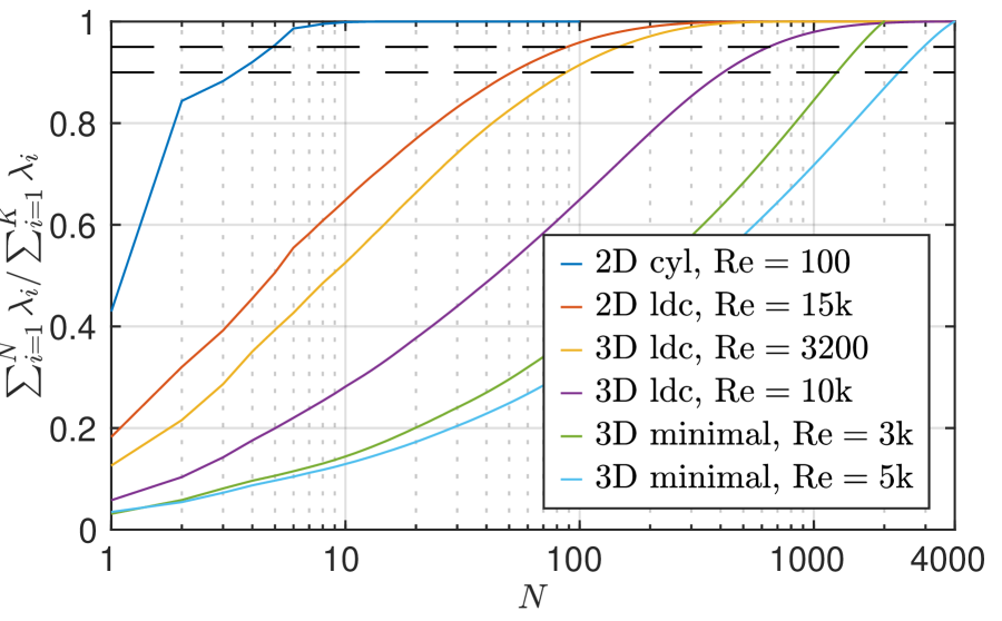
(a)

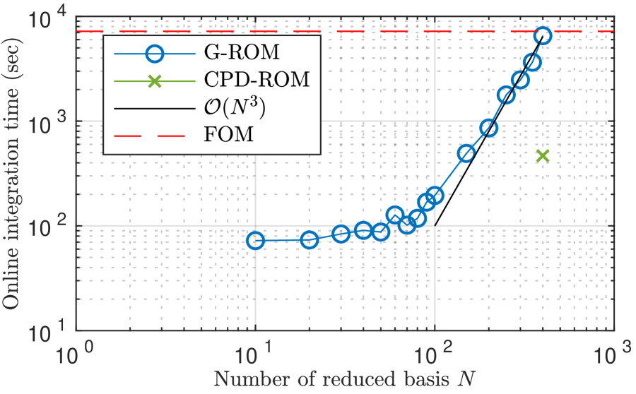
(b)

Figure 3.1: (a): Behavior of the accumulated POD eigenvalues for 2D periodic flow to 3D turbulent flows. Here CYL, LDC and MFU are denoted as flow past a cylinder, lid-driven cavity and minimal flow unit. (b): Behavior of the online solve time of the reduced system (2.8) as a function of $N$.

3.1 CPD-ROM

To address the $\mathcal{O}(N^{3})$ bottleneck, we consider CP decomposition to approximate the convection tensor $\mathcal{C}$ (2.7):

$$\mathcal{C}_{ikj}\approx\tilde{\mathcal{C}}_{ikj}=\sum^{R}_{r=1}a_{ir}b_{kr}c_{jr}.$$ (3.1)

With (3.1), the tensor contraction $\mathcal{C}({\underline{u}}){\underline{u}}$ is approximated by three matrix-vector multiplications :

$$\left[\mathcal{C}({{\underline{u}}}){{\underline{u}}}\right]_{i}\approx\left[\tilde{\mathcal{C}}({{\underline{u}}}){{\underline{u}}}\right]_{i}=\sum^{N}_{j=0}\sum^{N}_{k=0}\sum^{R}_{r=1}a_{ir}b_{kr}c_{jr}{u}_{k}{u}_{j}=\sum^{R}_{r=1}a_{ir}(\sum^{N}_{k=0}b_{kr}{u}_{k})(\sum^{N}_{j=0}c_{jr}{u}_{j}),\quad\forall~{}i=1,\ldots,N.$$ (3.2)

The cost is therefore reduced by a factor of $2N^{3}/6NR=N^{2}/3R$ in the leading order cost term. Throughout the paper, CPD-ROM is referred as the G-ROM Equation 2.8 with the approximated tensor $\tilde{\mathcal{C}}$ (3.1).

3.2 Partially skew-symmetric ROM tensor

In this subsection, we adapt the analysis in [58] and show that the ROM tensor Equation 2.7 is skew-symmetric in mode-$1$ and mode-$3$ with appropriate boundary and divergence-free conditions.

We begin with the definition of the ROM tensor Equation 2.7. Because each POD basis is a vector field $\bm{\varphi}_{i}=(\varphi_{i,x},\varphi_{i,y},\varphi_{i,z})$, Equation 2.7 can be further decomposed into three terms Equation 3.3, which represents the $x$-, $y$- and $z$- direction’s contribution, respectively:

$$\mathcal{C}_{ikj} =\int_{\Omega}\bm{\varphi}_{i}\cdot(\bm{\varphi}_{k}\cdot\nabla)\bm{\varphi}_{j}\,dV=\int_{\Omega}\varphi_{i,x}(\bm{\varphi}_{k}\cdot\nabla)\varphi_{j,x}~{}d\Omega+\int_{\Omega}\varphi_{i,y}(\bm{\varphi}_{k}\cdot\nabla)\varphi_{j,y}~{}d\Omega+\int_{\Omega}\varphi_{i,z}(\bm{\varphi}_{k}\cdot\nabla)\varphi_{j,z}~{}d\Omega.$$ (3.3)

Without loss of generality, we consider the $x$-direction contribution. With the divergence theorem and the product rule, the following equation is derived:

$$\int_{\Omega}\varphi_{i,x}(\bm{\varphi}_{k}\cdot\nabla)\varphi_{j,x}~{}d\Omega=-\int_{\Omega}\varphi_{j,x}(\bm{\varphi}_{k}\cdot\nabla)\varphi_{i,x}~{}d\Omega-\int_{\Omega}\varphi_{i,x}\varphi_{j,x}(\nabla\cdot\bm{\varphi}_{k})~{}d\Omega+\int_{\partial\Omega}\varphi_{i,x}\varphi_{j,x}\bm{\varphi}_{k}\cdot\hat{n}dA.$$ (3.4)

where $\hat{{{\bf n}}}$ is the outward unit normal on the boundary $\partial{\Omega}$. If the model problem has Dirichlet or periodic boundary conditions and the velocity reduced basis $\bm{\varphi}_{k}$ is divergence-free, i.e., $\nabla\cdot\bm{\varphi}_{k}=0$, the last two integrals vanish, leading to

$$\int_{\Omega}\varphi_{i,x}(\bm{\varphi}_{k}\cdot\nabla)\varphi_{j,x}~{}d\Omega=-\int_{\Omega}\varphi_{j,x}(\bm{\varphi}_{k}\cdot\nabla)\varphi_{i,x}~{}d\Omega.$$ (3.5)

This indicates that the $x$-direction contribution is skew-symmetric in mode-$1$ and mode-$3$. For the $y$- and $z$-direction contributions, a similar equations of (3.4)–(3.5) can be derived. Therefore, the ROM tensor Equation 2.7 is skew-symmetric.

Remark 3.1.

If the problem has inflow and outflow boundary conditions, the skew-symmetry no longer holds.

Remark 3.2.

In the case where skew-symmetry is no longer hold, the tensor $\mathcal{C}$ could always be decomposed into a skew-symmetric tensor plus a low-rank tensor contributed from the boundaries, i.e., the third term in (3.4).

Remark 3.3.

Even if the model problem has appropriate boundary conditions, the ROM tensor Equation 2.7 will not be exactly partially skew-symmetric because the divergence-free condition $\nabla\cdot\bm{\varphi}_{k}=0$ is not satisfied exactly. This is because each snapshot (FOM solution) only satisfied the divergence free condition in the weak form and the condition is enforced to a certain accuracy ($10^{-6}$–$10^{-8}$) only in practice. Therefore, divergence error (albeit small) will be present. In this case, we enfore the partially skew-symmetry by doing $\mathcal{C}_{ijk}=0.5(\mathcal{C}_{ijk}-\mathcal{C}_{kji})$ for all $i,j,k=1,\ldots,N$.

3.3 CP decomposition for partially skew-symmetric tensor

Skew-symmetric tensor also arises in many fields, for example, solid-state physics [41, 73], fluid dynamics [58], and quantum chemistry [54, 56, 72]. A tensor is skew-symmetric if its elements alternates sign under any permutation of the indices [70]. Tensors can be partially skew-symmetric in two or more modes as well.

Tensor decomposition for skew-symmetric tensor has been widely studied, see [51] for Tucker decomposition, and [4, 32, 33, 55] for decomposition into directional components (DEDICOM) and its applications. On the other hand, CP decomposition for the skew-symmetric tensor has not been widely studied, in fact, we could only find one related work [7] but with a different approach on enforcing skew-symmetry.

Assume the tensor $\mathcal{X}$ is skew-symmetric in mode-$1$ and mode-$3$, its CP decomposition is skew-symmetric if it satisfies:

$$\mathcal{X}\approx\llbracket A^{(1)},A^{(2)},A^{(3)}\rrbracket=\llbracket-A^{(3)},A^{(2)},A^{(1)}\rrbracket.$$ (3.6)

We impose the following conditions on the CP rank and factor matrices so that Equation 3.6 is satisfied:

$$\text{CP rank $R$ has to be even,}\quad\text{and}\quad A^{(1)}\equiv\left[A^{(1)}_{1}~{}A^{(1)}_{2}\right],~{}A^{(2)}\equiv\left[A^{(2)}_{1}~{}A^{(2)}_{1}\right],~{}A^{(3)}\equiv\left[A^{(1)}_{2}~{}-A^{(1)}_{1}\right],$$ (3.7)

where $A^{(1)}_{1}$ and $A^{(1)}_{1}$ are of size $N\times R/2$, and the factor matrix $A^{(2)}$ has $N/2$ redundant columns. With Equation 3.7, the CP decomposition can be expressed as:

$$\mathcal{X}\approx\llbracket A^{(1)},A^{(2)},A^{(3)}\rrbracket=\llbracket A^{(1)}_{1},A^{(2)}_{1},A^{(1)}_{2}\rrbracket+\llbracket A^{(1)}_{2},A^{(2)}_{1},-A^{(1)}_{1}\rrbracket=\llbracket-A^{(3)},A^{(2)},A^{(1)}\rrbracket,$$ (3.8)

and is skew-symmetric in mode-$1$ and mode-$3$.

The factor $A^{(2)}$ is computed as in ALS. For $A^{(1)}$ and $A^{(3)}$, we use an iterative algorithm [39] similar to the Babylonian square root algorithm, which updates $A^{(1)}$ using a series of subiterations. At each subiteration, a linear least squares problem is solved for $A^{(1)}$ with $A^{(3)}$ fixed,

$$A^{(1)}_{\text{next}}=\underset{B}{\mathrm{argmin}}\|\mathcal{X}-\llbracket B,A^{(2)},A^{(3)}\rrbracket\|_{F}.$$ (3.9)

Then both the first and third factors are updated with momentum, $A^{(1)}_{\text{new}}=\lambda A^{(1)}+(1-\lambda)A^{(1)}_{\text{next}}$, and $A^{(3)}_{\text{new}}=\begin{bmatrix}A^{(1)}_{\text{new},2}&-A^{(1)}_{\text{new},1}\end{bmatrix}$.

3.4 Underlying CP structure in the ROM tensor

In this section, we demonstrate that CP decomposition is a reasonable low-rank approximation for the advection tensor $\mathcal{C}$ (2.7) by showing there is an underlying CP structure. To see this, recall the definition of $\mathcal{C}$ (2.7) and substitute $\bm{\varphi}_{i},~{}\bm{\varphi}_{j}$ and $\bm{\varphi}_{k}$ with $\bm{\varphi}_{*}=(\varphi_{*,x},\varphi_{*,y})$,

$$\mathcal{C}_{ikj} =\int_{\Omega}\bm{\varphi}_{i}\cdot(\bm{\varphi}_{k}\cdot\nabla)\bm{\varphi}_{j}\,d\Omega=\int_{\Omega}\varphi_{i,x}(\bm{\varphi}_{k}\cdot\nabla)\varphi_{j,x}~{}d\Omega+\int_{\Omega}\varphi_{i,y}(\bm{\varphi}_{k}\cdot\nabla)\varphi_{j,y}~{}d\Omega$$

$$=\int^{1}_{-1}\int^{1}_{-1}\left(\varphi_{i,x}\varphi_{k,x}\frac{\partial\varphi_{j,x}}{\partial x}+\varphi_{i,x}\varphi_{k,y}\frac{\partial\varphi_{j,x}}{\partial y}+\varphi_{i,y}\varphi_{k,x}\frac{\partial\varphi_{j,y}}{\partial x}+\varphi_{i,y}\varphi_{k,y}\frac{\partial\varphi_{j,y}}{\partial y}\right)~{}dxdy.$$ (3.10)

For simplicity, we assume the problem is two-dimensional and the domain is simply $\Omega=[-1,~{}1]^{2}$ with one spectral element. For the general form with deformed geometry and multiple elements, we suggest [53] for a detailed review.

(3.10) is used to compute each component of the tensor $\mathcal{C}_{ikj}$ and the two-dimensional integration is computed using Gaussian quadrature:

$$\int^{1}_{-1}\int^{1}_{-1}\varphi_{i,x}\varphi_{k,x}\frac{\partial\varphi_{j,x}}{\partial x}~{}dxdy \simeq\sum^{q+1}_{m=1}\sum^{q+1}_{n=1}\omega_{m}\omega_{n}\varphi_{i,x}(\xi_{m},\xi_{n})\varphi_{k,x}(\xi_{m},\xi_{n})\frac{\partial\varphi_{j,x}(\xi_{m},\xi_{n})}{\partial x},$$ (3.11)

where $\{\omega_{i}\}^{q+1}_{i=1}$ and $\{\xi_{i}\}^{q+1}_{i=1}$ are the Gauss-Lobatto-Legendre (GLL) quadrature weights and points. Notice that, with $q+1$ GLL quadrature weights and points, the approximated integration is exact if the integrand is a polynomial of at most $2q-1$. However, the overall polynomial order inside the integral is larger than $2q-1$. Usually the exactness of (3.11) is enforced by interpolating the polynomial function onto a finer polynomial space of order $M=3q/2$, denoted as dealiasing [58]. Dealiasing increases the cost for evaluating (3.11) but the representation stays the same because eventually it is projected back to the original polynomial space of order $q$.

(3.11) suggests there is an underlying CP structure:

$$\int^{1}_{-1}\int^{1}_{-1}\varphi_{i,x}\varphi_{k,x}\frac{\partial\varphi_{j,x}}{\partial x}~{}dxdy =\sum^{q+1}_{m=1}\sum^{q+1}_{n=1}\omega_{m}\omega_{n}\varphi_{i,x}(\xi_{m},\xi_{n})\varphi_{k,x}(\xi_{m},\xi_{n})\frac{\partial\varphi_{j,x}(\xi_{m},\xi_{n})}{\partial x}$$

$$=\sum^{(q+1)^{2}}_{l=1}\rho_{l}a_{i,l}b_{k,l}c_{j,l},$$ (3.12)

where

$$\rho_{l}:=\omega_{m}\omega_{n},\quad a_{i,l}:=\varphi_{i,x}(\xi_{m},\xi_{n}),\quad b_{k,l}:=\varphi_{k,x}(\xi_{m},\xi_{n}),\quad\text{and}\quad c_{j,l}:=\frac{\partial\varphi_{j,x}(\xi_{m},\xi_{n})}{\partial x},$$ (3.13)

with the index $l:=m+(n-1)(q+1)$. The analysis can be applied to the other three terms in Equation 3.10 and a similar form of (3.12) can be derived. (3.12) suggests a theoretical bound of the CP rank of the advection tensor to be $4E(q+1)^{2}$ and $9E(q+1)^{2}$ for 2D and 3D problems, respectively, with $E$ being the number of spectral elements.

4 Numerical results

In this section, we present numerical results for the CPD-ROM introduced in Section 3.1. For comparison purposes, we also present the results of G-ROM (2.8) and the FOM. The ROM is constructed through an offline-online procedure: In the offline phase, the FOM is solved using the open-source code, Nek5000/RS [27, 29]. The POD basis and the reduced operators (2.7–2.10) are then constructed using NekROM. In addition, the CP decomposition for the tensor $\mathcal{C}$ is also carried out in the offline phase. In the online phase, the reduced system (2.8) is formed by loading the reduced operators and the CP factor matrices and solved using Matlab. We acknowledge there are high-performance tools for tensor decomposition with various optimization methods for example [70], however, the primary focus of this paper is the application of the tensor decomposition with ROM, hence we implement CP-ALS (2.13) and CP-ALS with quadratically-occuring factors (3.9) in Matlab for easy use and investigation with ROM. We use the campus cluster Delta and Argonne Leadership Computing Facility (ALCF) Polaris for the offline stage and a workstation with Intel Xeon E5-2620 CPU with 2 threads for the CP decomposition and solving the reduced system.

From the numerical investigation, we would like to address following questions:

• Without sacrificing too much accuracy, is there any memory saving and speed-up with CPD-ROM?

• Does preserving the skew-symmetry property in the approximated tensor stabilize CPD-ROM?

• Does the advection tensor $\mathcal{C}$ have low-rank structure and how does it relate to the parameters such as the number of POD modes $N$, the Reynolds number $\rm Re$, the spatial dimension $d$, the norm used to construct the POD basis?

The rest of this section is organized as follows: In Section 4.1, we compare the CPD-ROM with the G-ROM in four model problems, ranging from 2D chaotic flow to 3D turbulent flows. In Section 4.2, we investigate the performance of the CPD-ROM with the approximated full tensor and the approximated core tensor. In Section 4.3, we investigate if preserving the skew-symmetry for the approximated tensor is beneficial for the CPD-ROM. In Section 4.4, we investigate the G-ROM with singular value decomposition (SVD). In Section 4.4.1, we investigate the low-rank structure of the tensor under the $L^{2}$ and $H^{1}_{0}$ norms using the SVD. Additionally, we investigate the effectiveness of the low-rank approximation between the SVD and CPD. In Section 4.4.2, we compare the performance of the CPD-ROM with the SVD-ROM, i.e., the G-ROM with the singular value decomposition (SVD). Finally, we employ the $H^{1}_{0}$-based POD basis for both the G-ROM and CPD-ROM across our study. This selection is motivated by the low-rank structure identified with the $H^{1}_{0}$ norm, as discussed in Section 4.4.1.

4.1 Performance comparison between the G-ROM and the CPD-ROM

In this section, we compare the performance of the CPD-ROM (Section 3.1) with the G-ROM (2.8) and the FOM across various model problems: 2D flow past a cylinder, 2D lid-driven cavity, 3D lid-driven cavity, and 3D minimal flow unit. The comparison is based on the accuracy of the quantities of interest (QOIs).

The compression ratio (CR) of the ALS (2.13) and ALS-quad (3.9) are defined based on the ratio of sizes of the original tensor and the size of the CPD models:

$$\text{CR}_{\text{ALS}}=\frac{N^{3}}{3NR}=\frac{N^{2}}{3R},\quad\text{CR}_{\text{ALS-quad}}=\frac{N^{3}}{\frac{3}{2}NR}=\frac{2N^{2}}{3R}.$$ (4.1)

A factor of $2$ emerges in $\text{CR}_{\text{ALS-quad}}$ due to the presence of redundant columns in the factor matrix $A^{(2)}$ and the skew-symmetric structure in $A^{(1)}$ and $A^{(3)}$ (Section 3.3). These compression ratios ignore the skew-symmetry of the original tensor, since its is difficult to exploit in storage or application of the operator (tensor contraction). Notice that the cost reduction in tensor contraction with ALS-quad is the same as with ALS, i.e., $N^{2}/3R$, as it still involves three matrix-vector multiplications (3.2)

4.1.1 2D flow past a cylinder

Our first example is the 2D flow past a cylinder at the Reynolds number $\rm Re=100$, which is a canonical test case for ROMs due to its robust and low-dimensional attractor, manifesting as a von Karman vortex street for $\rm Re=UD/\nu>34.37$ [20]. The computational domain is $\Omega=[-2.5:17]D\times[-5:5]D$, with the unit-diameter cylinder centered at $[0,0]$.

The reduced basis $\{\bm{\varphi}_{i}\}^{N}_{i=1}$ for the G-ROM (2.6) is constructed by applying POD procedure to $K=100$ snapshots collected over $100$ convective time units $(D/U)$, after von Karman vortex street is developed. The zeroth mode $\bm{\varphi}_{0}$ is set to be the mean velocity field of the snapshot collection time window. Already with $N=20$ POD basis, the reduced space contains more than $99\%$ of the total energy of the snapshots. The initial condition for the G-ROM and the CPD-ROM is obtained by projecting the lifted snapshot at $t=500$ (in convective time units) onto the reduced space.

We test the CPD-ROM in the reconstructive regime, ie., the same time interval in which the snapshots were collected. The total drag on the cylinder is defined as:

$$\bm{F}_{D}=\oint_{\Gamma}(-\nu\nabla{\bm{u}}+p)d{\bm{A}},$$ (4.2)

where $\Gamma$ is the surface of the cylinder. We consider the total drag in the $x$-direction as the QOI. We refer to [44] for computing the pressure drag in the ROM without solving the pressure solution.

Fig. 1(a) displays the relative error in the mean drag and its standard deviation of CPD-ROM with respect to both the FOM and the G-ROM as a function of the CP rank $R$. Additionally, it includes the relative error of the G-ROM’s results with respect to the FOM for comprehensive comparison. We found the error with respect to the G-ROM decreases as $R$ increases. With $R\geq 200$, the error in both the mean and standard deviation is less than $10^{-8}$, indicating the convergence of CPD-ROM to G-ROM. With respect to the FOM, the error decreases initially as $R$ increases and eventually reaches to the same level of accuracy as G-ROM (blue dashed line). This is expected because G-ROM serves as the reference model for the CPD-ROM.

Fig. 1(b) shows the total drag history of CPD-ROM at $R=10$ and $R=50$ alongside G-ROM and FOM results. We found with $R=10$, despite the inaccuracy in the approximated tensor, the total drag of CPD-ROM does not blow up and reaches a constant value eventually. This behavior could be attributed to the model problem having a robust and low-dimensional attractor. With $R=50$, the total drag of CPD-ROM shows good agreement with the results of both FOM and G-ROM.

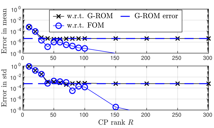
(a) Relative error in mean drag and its standard deviation

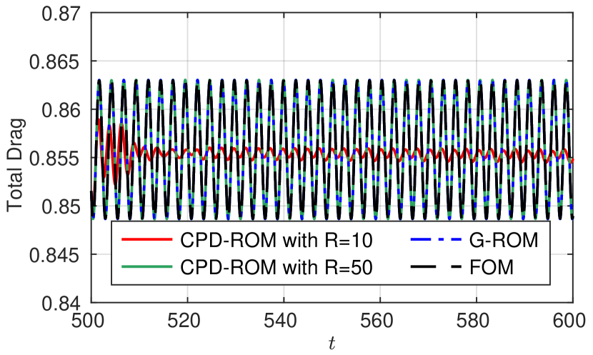
(b) Drag history

Figure 4.1: 2D flow past a cylinder at $\rm Re=100$: (a) Relative error in the mean drag and its standard deviation as a function of the CP rank $R$. The error is presented with respect to both the FOM and G-ROM for each quantity. The relative error of the G-ROM’s results with respect to the FOM is also illustrated as a blue dashed line. (b) The total drag history of CPD-ROM at $R=10$ and $R=50$, along with the results of the FOM and the G-ROM. The number of POD modes, $N$, is set to $20$ for both the G-ROM and the CPD-ROM.

4.1.2 2D lid-driven cavity

Our next example is the 2D lid-driven cavity (LDC) problem at $\rm Re=15,000$, which is a more challenging model problem compared to the 2D flow past a cylinder. As demonstrated in [25], the problem requires $N\geq 60$ POD modes for G-ROM to accurately reconstruct the solutions and QOIs. A detailed description on how the FOM is set up for this problem can be found in our previous work [45].

The reduced basis $\{\bm{\varphi}_{i}\}^{N}_{i=1}$ is constructed by applying POD to $K=2000$ snapshots in the statistically steady state region in the time interval of $[6000.4,~{}6200]$ with sampling time $\Delta t_{s}=0.1$. The zeroth mode $\bm{\varphi}_{0}$ is set to the mean velocity field of the snapshot collection time window. The initial condition for the G-ROM and the CPD-ROM is obtained by projecting the lifted snapshot at $t=6000$ (in convective time units) onto the reduced space.

We test both G-ROM and CPD-ROM in the reconstructive regime with $N=200$ for both models. The choice of $N=200$ ensures that the G-ROM is accurate compared to the FOM. In terms of the QOI, we consider the energy and the energy of the fluctuated velocity:

$$\mathrm{E}(t)=\frac{1}{2}\int_{\Omega}\|{\bm{u}}(x,t)\|^{2}_{2},\quad\mathrm{E}(t)_{\text{fluc}}=\frac{1}{2}\int_{\Omega}\|{\bm{u}}(x,t)-\langle{\bm{u}}\rangle(x)\|^{2}_{2},$$ (4.3)

where $\|\cdot\|_{2}$ is the Euclidean norm.

Fig. 2(a) displays the relative error in the mean energy and its standard deviation of CPD-ROM with respect to both the FOM and the G-ROM as a function of the CP rank $R$. Additionally, it includes the relative error of the G-ROM’s results with respect to the FOM.

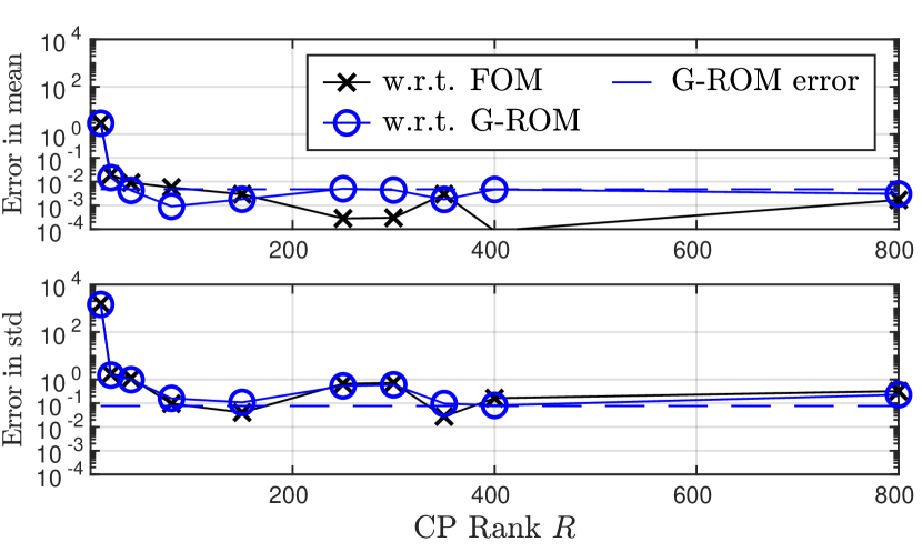
(a) Relative error in mean energy and its standard deviation

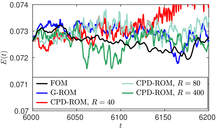
(b) Energy history

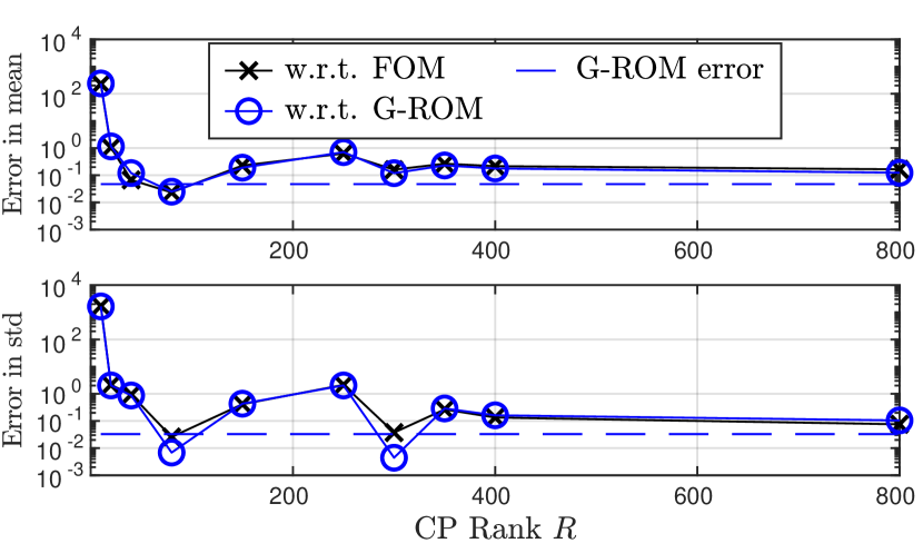
(c) Relative error in mean $\mathrm{E}_{\text{fluc}}$ and its standard deviation

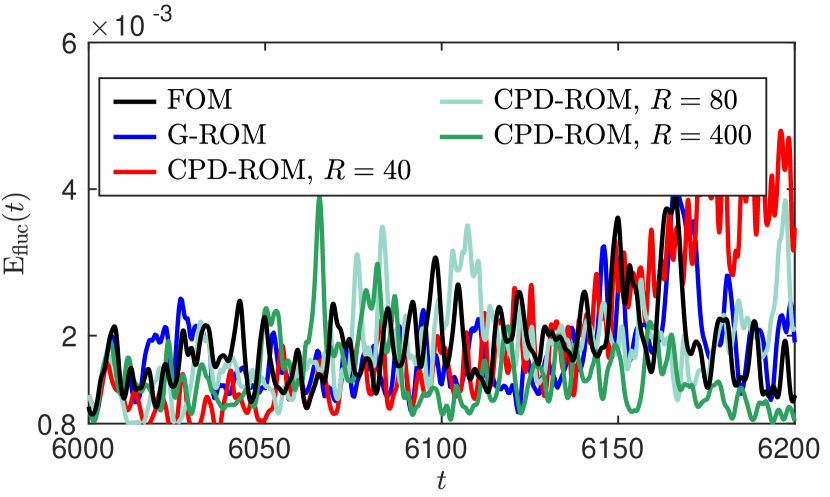
(d) $\mathrm{E}_{\text{fluc}}$ history

Figure 4.2: 2D lid-driven cavity at $\rm Re=15000$: Relative error in both (a) mean and standard deviation of the energy and (c) mean and the standard deviation of the energy of the fluctuated velocity as a function of the CP rank $R$. The error is presented with respect to both the FOM and G-ROM for each quantity. The relative error of the G-ROM’s results with respect to the FOM is also illustrated as a blue dashed line; The (b) energy and (d) energy of the fluctuated velocity history of CPD-ROM at $R=80$ and $400$, along with the results of the FOM and the G-ROM. The number of POD modes, $N$, is set to $200$ for both the G-ROM and the CPD-ROM.

Unlike the results of 2D flow past a cylinder, where the error with respect to G-ROM decreases to machine precision as $R$ increases, we found the error (orange) decreases as $R$ increases and starts fluctuating at the level of G-ROM’s accuracy (black solid line) after $R\geq 80$. It is not surprising to find this because the model problem itself is much more chaotic compared to the 2D flow past a cylinder, and any approximation error could lead to a different solution trajectory. On the other hand, we found the error with respect to the FOM decreases as $R$ increases and eventually reach to the same level of accuracy as G-ROM (black solid line), as in the case of 2D flow past a cylinder. In fact, we found the error in mean of CPD-ROM is smaller than the error of G-ROM with $R\geq 250$.

We further plot the energy history of CPD-ROM with $R=80$ and $R=400$, which both have error less than $0.1\%$ in mean and about $10\%$ in the standard deviation in Fig. 2(b), along with the results of the FOM and the G-ROM. In both $R$ values, we found the energy of CPD-ROM initially agree with the G-ROM and depart to a different trajectory at $t\approx 6010$. This is expected due to the approximation error made in the CP decomposition.

Fig. 2(c) displays the relative error in the mean energy of the fluctuated velocity and its standard deviation of CPD-ROM with respect to both the FOM and the G-ROM as a function of the CP rank $R$. Further, it includes the relative error of the G-ROM’s results with respect to the FOM. We found a similar error behavior as in the results of energy but with higher errors in general. This is expected because the energy of the fluctuated velocity is a much harder QOI compared to the energy. In addition, we also found the error of the CPD-ROM with respect to the FOM is in general larger than G-ROM’s error. Moreover, we are aware of an increase in the error when increasing $R$ from $80$ to $300$. We suspect this error behavior is due to the random initial condition in the CP decomposition. Hence, we further run five more trials of the CP decomposition for $R=80,~{}150,~{}250$ and $300$. We do not find small error at $R=80$ as in Fig. 2(c) but find the error decrease in general as $R$ increases.

We plot the energy of the fluctuated velocity history of CPD-ROM with $R=80$ and $R=400$ in Fig. 2(b), along with the results of the FOM and the G-ROM. Again, in both $R$ values, we found the energy of CPD-ROM initially agree with the G-ROM and depart to a different trajectory at $t\approx 6010$.

In terms of the energy, CPD-ROM with $R=80$ is sufficient to attain the same level of accuracy as in the G-ROM for the mean and the standard deviation. The compression ratio is $\text{CR}=333.3$ and the cost of evaluating the nonlinear term is reduced by a factor of $166.6$. In terms of the energy of the fluctuated velocity, CPD-ROM with $R=300$ is able to attain the same level of accuray as in the G-ROM for the standard deviation and a factor of $4$ in the error of the mean. The compression ratio is $\text{CR}=66.7$ and the cost of evaluating the nonlinear term is reduced by a factor of $33.3$.

Finally, for $200,000$ time steps, the total solve time of the G-ROM with $N=200$ is about $1167$ (secs) and the tensor contraction kernel occupies about $86\%$ of the total solve time whereas, the total solve time of the CPD-ROM with $R=300$ is about $101$ (secs) and the CP kernel (3.2) occupies only $15\%$ of the total solve time. With a factor of $44.4$ in reduction, we should observe a factor of $6.25$ speedup in the total solve time. In fact, from the numbers reported here, we get a factor of $11.5$ speedup. We note this is due the favorable cache effect. The machine used to run the G-ROM and CPD-ROM has a L1 cache of size $0.384$ megabyte (MB), a L2 cache of size $3$ MB and a L3 cache shared by all cores of size $30$ MB. With $N=200$, the advection tensor $\mathcal{C}$ is of size $210$ MB, whereas the total size of the factor matrices are $4.5$ MB with $R=300$. The additional speedup is because in the case of CPD-ROM, there is sufficient space in the L3 cache to store the ROM operators. We note that, the numbers reported here are based on the results running with one computing thread in Matlab. We choose to apply this constraint because Matlab optimizes the G-ROM when $N$ is large due to large tensor whereas no optimization is used for the CPD-ROM.

4.1.3 3D lid-driven cavity (LDC)

We next consider the non-regularized 3D lid-driven cavity (LDC) problem as our first 3D example, which is a much more challenging model problem for the ROM compared to the 2D problems. We consider two Reynolds number, i.e., $\rm Re=3200$ and $\rm Re=10,000$. Following [44], for both $\rm Re$, the FOM mesh consists of a tensor-product array of $E=16^{3}$ elements with a Chebyshev distribution with polynomial order $7$, leading to a total of $2$ million unkowns. We found the results of $\rm Re=3200$ and $\rm Re=10,000$ are qualitatively similar and show the results of $\rm Re=10,000$ because higher Reynolds number is more interesting. We refer the dissertation [74] for the results of $\rm Re=3200$.

The reduced basis $\{\bm{\varphi}_{i}\}^{N}_{i=1}$ is constructed with POD using $K=4000$ snapshots in the statistically steady state region in the time interval of $[2725.125,~{}3225]$ with sampling time $\Delta t_{s}=0.125$. The zeroth mode $\bm{\varphi}_{0}$ is set to the mean velocity field of the snapshot collection time window. The initial condition for the G-ROM and the CPD-ROM is obtained by projecting the lifted snapshot at $t=2725$ onto the POD space.

We test the G-ROM and CPD-ROM in the predictive regime, i.e., a larger time interval compared to the interval snapshots are collected. We consider $N=400$ for both models and the choice of the $N$ value ensures that the G-ROM is accurate compared to the FOM. We consider the energy and the energy of the fluctuated velocity, defined in (4.3), as the QOIs.

Fig. 3(a) displays the relative error in the mean energy and its standard deviation of CPD-ROM with respect to both the FOM and the G-ROM as a function of the CP rank $R$. Additionally, it includes the relative error of the G-ROM’s results with respect to the FOM. We found the error with respect to both the FOM and the G-ROM decreases as $R$ increases. In addition, we find at least $R\geq 1600$ is required for CPD-ROM to predict the mean with an error of $10\%$ and in order to predict a reasonable standard deviation, $R=3200$ is required. We plot the energy history in CPD-ROM with $R=1600$ and $R=3200$ in Fig. 3(b), along with the results of the FOM and the G-ROM. We found the result with $R=1600$ has much larger fluctuation compared to the FOM and the G-ROM and observed an improvement with $R=3200$.

Fig. 3(c) displays the relative error in the mean energy of the fluctuated velocity and its standard deviation of CPD-ROM with respect to both the FOM and the G-ROM as a function of the CP rank $R$. We found a similar error behavior as in the results of energy but with larger relative errors of the G-ROM in both quantities. In fact, with $R=3200$, CPD-ROM is able to predict the standard deviation with same level of accuracy as of G-ROM and predict the mean more accurately than the G-ROM.

We plot the energy of the fluctuated velocity history in CPD-ROM with $R=1600$ and $3200$ in Fig. 3(d), along with the FOM and G-ROM results. The results with $R=3200$ is similar to those of the G-ROM and the FOM while the results with $R=1600$ has larger fluctuation.

In summary, in order to predict the mean energy with an error less than $10\%$, $R=1600$ is required for the CPD-ROM. For the mean energy of the fluctuated velocity, a larger CP rank, $R=3200$, is required. In order to predict the standard deviation with an error less than $10\%$, $R>3200$ is required. With $N=400$ and $R=3200$, the compression ratio is $\text{CR}=33.3$ and the cost is reduced by a factor of $16.7$. Finally, for $1,000,000$ time steps, the total solve time of the G-ROM with $N=400$ is about $43819$ (secs) and the tensor contraction kernel occupies about $97\%$ of the total solve time whereas, the total solve time of the CPD-ROM with $R=3200$ is about $4269$ (secs) and the CP kernel (3.2) occupies only $64.8\%$ of the total solve time. We get a factor of $10.3$ speedup in the total solve time which is close to the theoretical speedup $11.4$ with a factor of $16.7$ in reduction. We do not get a larger speedup as in the previous model problem because the size of the factor matrices with $R=3200$ and $N=400$ is $91$ MB, which is larger than the L3 cache size.

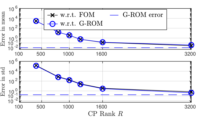
(a) Relative error in mean energy and its standard deviation

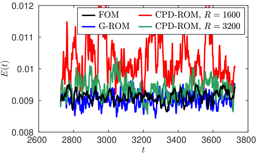
(b) Energy history

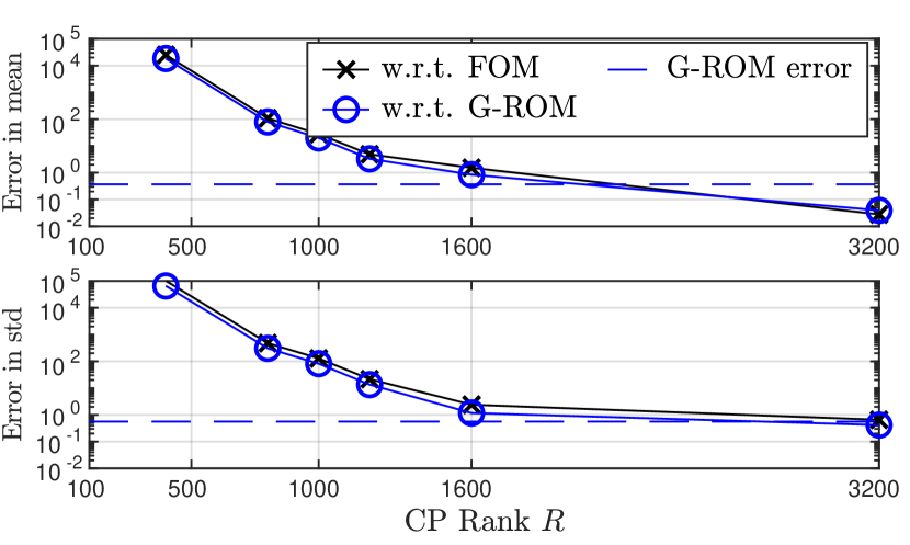
(c) Relative error in mean $\mathrm{E}_{\text{fluc}}$ and its standard deviation

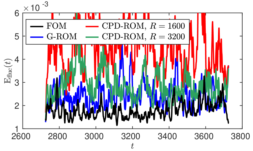
(d) $\mathrm{E}_{\text{fluc}}$ history

Figure 4.3: 3D lid-driven cavity at $\rm Re=10,000$: Relative error in both (a) mean and standard deviation of the energy and (c) mean and the standard deviation of the energy of the fluctuated velocity as a function of the CP rank $R$. The error is presented with respect to both the FOM and G-ROM for each quantity. The relative error of the G-ROM’s results with respect to the FOM is also illustrated as a blue dashed line; The (b) energy and (d) energy of the fluctuated velocity history of CPD-ROM at $R=3200$, along with the results of the FOM and the G-ROM. The number of POD modes, $N$, is set to $400$ for both the G-ROM and the CPD-ROM.

4.1.4 The minimal flow unit (MFU)

Our next 3D example is the minimal flow unit (MFU), which presents some strong turbulent features while maintaining simplified flow dynamics, resulting in significantly lower computational costs compared to a full channel flow simulation [42]. Following the setup in [42], we consider two Reynolds numbers $\rm Re$. For $\rm Re=3000$, the streamwise (i.e, the $x$-direction) and spanwise (i.e, the $z$-direction) lengths of the channel are set to $\pi h$ and $0.3\pi h$, respectively. For $\rm Re=5000$, the streamwise and spanwise lengths of the channel are set to $0.6\pi h$ and $0.18\pi h$, respectively. The channel half-height is set to $h=1$ for both $\rm Re$. For both $\rm Re$, the FOM mesh consists of an array of $8\times 18\times 4$ elements in the $x\times y\times z$ directions), of order $q=9$, for a total of ${\cal N}\approx 420$ thousands grid points. We found the results of $\rm Re=3200$ and $\rm Re=10,000$ are qualitatively similar and show the results of $\rm Re=10,000$ because higher Reynolds number is more interesting. We refer the dissertation [74] for the results of $\rm Re=3200$.

The reduced basis $\{\bm{\varphi}_{i}\}^{N}_{i=1}$ is constructed with POD using $K=4000$ snapshots in the statistically steady state region in the time interval of $[3000.125,~{}3500]$ with sampling time $\Delta t_{s}=0.125$. The zeroth mode $\bm{\varphi}_{0}$ is set to the mean velocity field of the snapshot collection time window. The initial condition for the G-ROM and the CPD-ROM is obtained by projecting the lifted snapshot at $t=3000$ onto the POD space.

We test the G-ROM and CPD-ROM in the predictive regime, i.e., a larger time interval compared to the interval snapshots are collected. We consider $N=400$ for both models and consider the energy and the energy of the fluctuated velocity, defined in (4.3), as the QOIs.

Fig. 4(a) displays the relative error in the mean energy and its standard deviation of CPD-ROM with respect to both the FOM and the G-ROM as a function of the CP rank $R$. We find at least $R\geq 1200$ is required for CPD-ROM to predict the mean with an error of $10\%$ and in order to predict a reasonable standard deviation, $R=3000$ is required. We also find the error with respect to the G-ROM decreases as $R$ increases whereas the error with respect to the FOM starts fluctuating around the level of G-ROM’s accuracy when $R\geq 2000$. The energy history in CPD-ROM with $R=2000$ and $R=4000$ is shown in Fig. 4(b), along with the results of the FOM and the G-ROM. We could see that the results of $R=4000$ is quite similar to the results of the FOM and the G-ROM whereas the results of $R=2000$ has a larger fluctuation.

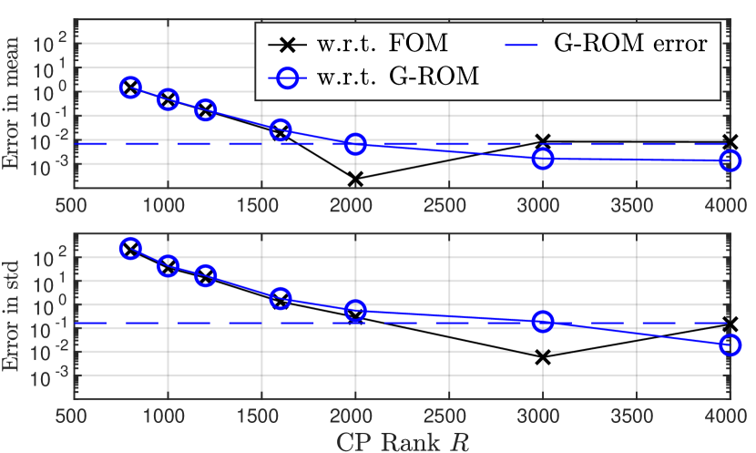
(a) Relative error in mean energy and its standard deviation

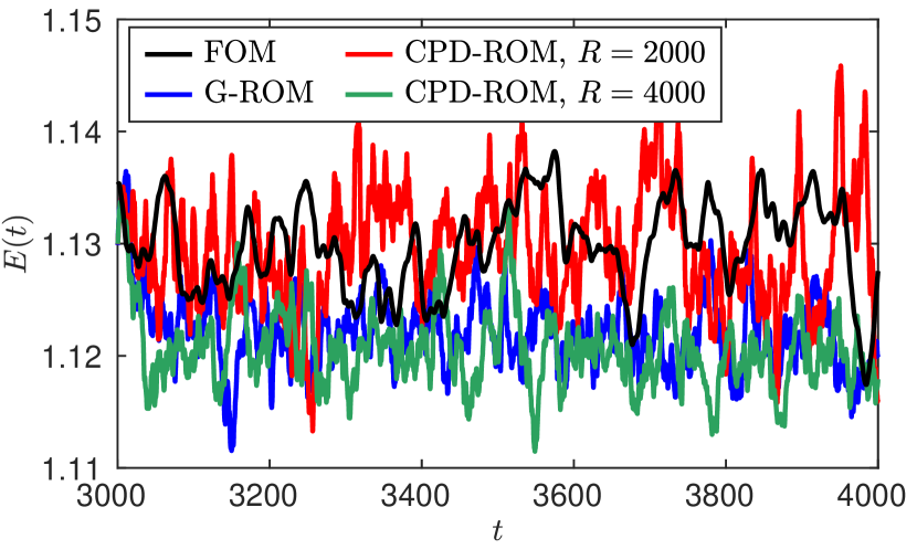
(b) Energy history

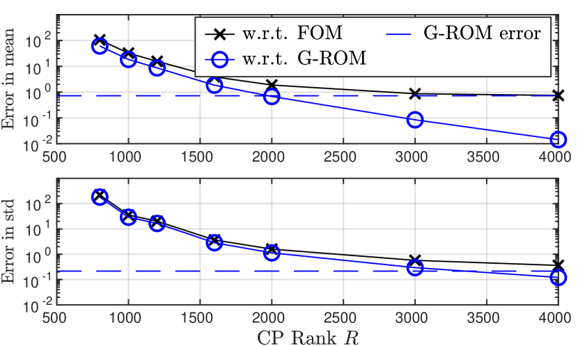
(c) Relative error in mean $\mathrm{E}_{\text{fluc}}$ and its standard deviation

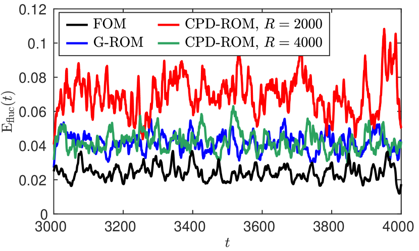
(d) $\mathrm{E}_{\text{fluc}}$ history

Figure 4.4: MFU at $\rm Re=5000$: Relative error in both (a) mean and standard deviation of the energy and (c) mean and the standard deviation of the energy of the fluctuated velocity as a function of the CP rank $R$. The error is presented with respect to both the FOM and G-ROM for each quantity. The relative error of the G-ROM’s results with respect to the FOM is also illustrated as a blue dashed line; The (b) energy and (d) energy of the fluctuated velocity history of CPD-ROM at $R=4000$, along with the results of the FOM and the G-ROM. The number of POD modes, $N$, is set to $400$ for both the G-ROM and the CPD-ROM.

Fig. 4(c) displays the relative error in the mean energy of the fluctuated velocity and its standard deviation of CPD-ROM with respect to both the FOM and the G-ROM as a function of the CP rank $R$. Again we observe both the error with respect to the FOM and the G-ROM decreases as $R$ increases and eventually reach to the level of G-ROM’s accuracy. However, the errors are large because the G-ROM itself is not accurate, with an error of $70\%$ and $21\%$ in the mean and the standard deviation. To further improve the results, $N>400$ is required for the G-ROM. The $\mathrm{E}_{\text{fluc}}$ history in the CPD-ROM with $R=2000$ and $R=4000$ are shown in Fig. 4(d), along with the results of the FOM and the G-ROM. We find that the results of $R=2000$ is not accurate and the results of $R=4000$ is quite similar to the results of the G-ROM however, both are inaccurate compared to the FOM.

In summary, CPD-ROM with $R\geq 3000$ is able to predict the mean energy and its standard deviation with error less than $10\%$. With $R=3000$, the compression ratio is of $26.6$ and the cost is reduced by a factor of $13.3$.

For the energy of the fluctuated velocity, despite CPD-ROM is able to reach to the same level of accuracy as G-ROM with $R=4000$, the errors with respect to the FOM are large ($>20\%$). This is due to the inaccuracy in G-ROM and to resolve this issue, one has to consider a larger $N$.

With $N=400$ and $R=3000$, the compression ratio is $\text{CR}=35.5$ and the cost is reduced by a factor of $17.7$. Finally, for $400,000$ time steps, the total solve time of the G-ROM with $N=400$ is about $17470$ (secs) and the tensor contraction kernel occupies about $97\%$ of the total solve time whereas, the total solve time of the CPD-ROM with $R=3000$ is about $1559$ (secs) and the CP kernel (3.2) occupies only $64.1\%$ of the total solve time. We get a factor of $11.2$ speedup in the total solve time which is close to the theoretical value $11.8$ with a factor of $17.7$ in reduction.

4.2 Performance investigation of CPD-ROM with the approximated full tensor and the approximated core tensor

In this section, we investigate the performance of the CPD-ROM with the approximated full tensor (CPD-ROM-Full) and the approximated core tensor (CPD-ROM-Core). Recall the definition of the advection tensor:

$$\mathcal{C}_{ikj}=\int_{\Omega}\bm{\varphi}_{i}\cdot(\bm{\varphi}_{k}\cdot\nabla)\bm{\varphi}_{j}~{}dV.$$ (4.4)

The full tensor includes the contribution from the zeroth mode $\bm{\varphi}_{0}$ and is defined as $\mathcal{C}_{ikj}$ with $i=1,\ldots,N$ and $j,k=0,\ldots,N$ whereas the core tensor does not have the zeroth mode contribution and is defined as $\mathcal{C}_{ikj}$ with $i,j,k=1,\ldots,N$.

Applying the CP decomposition to either the full tensor or the core tensor is valid. However, we expect CPD-ROM-Core outperforms the CPD-ROM-Full, because the zeroth mode contributions, which are the $C_{1}$ and $C_{2}$ matrices defined in (2.10), remains exact. For fair comparison, we consider ALS for both tensors.

Fig. 5(a) displays the energy history (4.3) of the CPD-ROM-Full and the CPD-ROM-Core at $R=350$ along with the results of FOM and the G-ROM. We found with $R=350$, the CPD-ROM-Core is able to reproduce the energy history with relative errors (with respect to the FOM) less than $0.1\%$ in the mean and $\approx 27\%$ in the standard deviation. On the other hand, the CPD-ROM-Full is not stable and its solution blows up after $t>6030$. Despite we found a significant performance difference between the CPD-ROM-Core and the CPD-ROM-Full with same rank $R$, the relative residual of the approximated tensor is similar in both case.

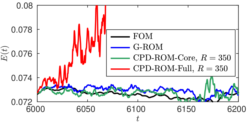
(a) Energy history

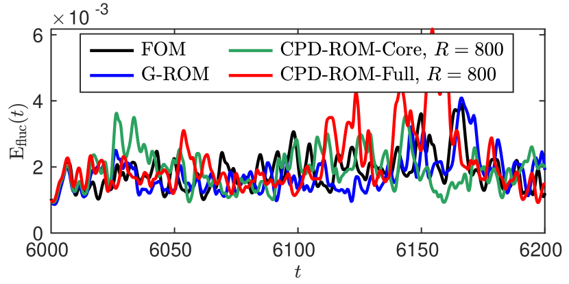
(b) $\mathrm{E}_{\text{fluc}}$ history

Figure 4.5: 2D lid-driven cavity at $\rm Re=15,000$: Comparison of (a) the energy history and (b) the energy of the fluctuated velocity $\mathrm{E}_{\text{fluc}}$ between the CPD-ROM-Full and the CPD-ROM-Core, along with the results of the FOM and the G-ROM. CPD-ROM-Full and CPD-ROM-Core are denoted as the CPD-ROM with the approximated full tensor and the approximated core tensor.

Fig. 5(b) displays the energy of the fluctuated velocity $\mathrm{E}_{\text{fluc}}$ history (4.3) of the CPD-ROM-Full and the CPD-ROM-Core at $R=800$ along with the results of FOM and the G-ROM. $\mathrm{E}_{\text{fluc}}$ is in general a much harder QOI compared to the energy and we found $R=800$ is necessary for the CPD-ROM-Core to be accurate. We found CPD-ROM-Core is much more accurate than the CPD-ROM-Full. Although the problem is chaotic, The $\mathrm{E}_{\text{fluc}}$ of CPD-ROM-Core behaves similarly compared to the FOM with relative errors of $4\%$ in both the mean and the standard deviation. On the other hand, the $\mathrm{E}_{\text{fluc}}$ of CPD-ROM-Full overshoots in later time with relative errors of $16\%$ in the mean and $71\%$ in the standard deviation.

We next investigate the performance of the CPD-ROM-Full and CPD-ROM-Core in the 3D lid-driven cavity at $\rm Re=3200$. We test both modes in the reconstructive and the predictive regimes.

(a) Reconstructive regime

(b) Predictive regime

Figure 4.6: 3D lid-driven cavity at $\rm Re=3200$: Comparison of the energy of the fluctuated velocity in (a) the reconstructive and (b) the predictive regimes between the CPD-ROM-Full and the CPD-ROM-Core, along with the results of the FOM and the G-ROM. CPD-ROM-Full and CPD-ROM-Core are denoted as the CPD-ROM with the approximated full tensor and the approximated core tensor.

Fig. 6(a) displays the $\mathrm{E}_{\text{fluc}}$ history of the CPD-ROM-Full and the CPD-ROM-Core in the reconstructive regime at $R=1600$ along with the results of FOM and the G-ROM. $R=1600$ is selected so that CPD-ROM-Core is accurate. We found that with $R=1600$, CPD-ROM-Core is able to reproduce the history with an error (with respect to the FOM) of $5\%$ in the mean and $0.4\%$ in the standard deviation. On the other hand, despite the solution of the CPD-ROM-Full does not blow up, it is less accurate, with an error of $9\%$ in the mean and $127\%$ in the standard deviation.

Fig. 6(b) displays the $\mathrm{E}_{\text{fluc}}$ history of the CPD-ROM-Full and the CPD-ROM-Core in the predictive regime at $R=1600$ along with the results of FOM and the G-ROM. We found CPD-ROM-Core is able to accurately predict the QOI with an error of $2\%$ in the mean and $5\%$ in the standard deviation. On the other hand, CPD-ROM-Full is not accurate, with an error of $10\%$ in the mean and $200\%$ in the standard deviation.

4.3 Performance investigation of the CPD-ROM with skew-symmetry preserved

In this section, we investigate if preserving the skew-symmetry for the approximated tensor ${\widehat{\mathcal{C}}}$ is beneficial for the performance of the CPD-ROM. We compare the performance of the CPD-ROM with skew-symmetry preserved (CPD-ROM-Skew) with the CPD-ROM without preserving the property (CPD-ROM) in the 2D and the 3D lid-driven cavity and the minimal flow unit (MFU). The selection of these model problems is deliberate, as they provide suitable boundary conditions for skew-symmetry (3.5). The ALS-skew, introduced in Section 3.3, is employed to ensure the skew-symmetry of the CP decomposition. Additionally, we enforce skew-symmetry in the tensor $\mathcal{C}$ itself, as discussed in Section 3.2.

Fig. 4.7 displays the results of the 2D lid-driven cavity at $\rm Re=15000$. In Fig. 7(a), we compare the relative errors in the mean energy and its standard deviation between the CPD-ROM-Skew and the CPD-ROM as a function of CP rank $R$. In the results of CPD-ROM, the circle marker with a cross marker at several $R$ values, indicate solution blow-up, resulting in NaN errors. We found CPD-ROM-Skew outperforms CPD-ROM for small $R$ values, and as $R$ increases, both behaves similarly. This behavior is expected because skew-symmetry addresses stability, not accuracy. This observation is consistent with the behavior of full-order models, where recovery of skew symmetry (e.g., through dealiasing) is known to provide stability but does not, in general, improve accuracy. This point was discussed in numerous early works by Orszag and co-authors (e.g., [30, 63, 64]).

In Fig. 7(b), we compare the energy history between the CPD-ROM-Skew and the CPD-ROM at $R=80$ and $R=400$, along with the results of the FOM and the G-ROM. At $R=80$, we found the CPD-ROM is not stable leading to blowing-up solutions whereas the CPD-ROM-Skew is stable and has errors of less than $1\%$ in mean and about $10\%$ in the standard deviation. At $R=400$, the approximated tensor is accurate enough so that CPD-ROM is stable.

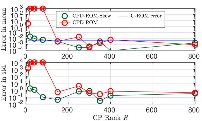
(a) Relative error in mean energy and its standard deviation

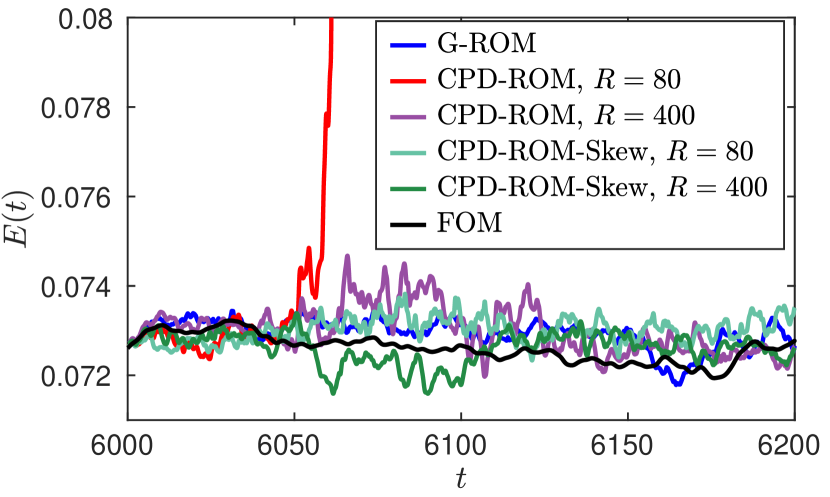
(b) Energy history

Figure 4.7: 2D lid-driven cavity at $\rm Re=15,000$: (a) Comparison of the relative error in both the mean and the standard deviation of the energy between CPD-ROM-Skew and CPD-ROM as a function of the CP rank $R$. The error is presented with respect to the FOM. The relative error of the G-ROM’s results with respect to the FOM is also illustrated as a blue dashed line. (b) Comparison of the energy history between CPD-ROM-Skew and CPD-ROM at $R=80$ and $R=400$, along with the results of the FOM and the G-ROM. CPD-ROM-Skew is denoted as CPD-ROM with skew-symmetry preserved. The circle marker with a cross marker at several $R$ values, indicate solution blow-up, resulting in NaN errors.

Fig. 4.8 displays the results of the 3D lid-driven cavity. In Figs. 8(a)–8(b), we compare the relative errors in the mean energy and its standard deviation between the CPD-ROM-Skew and the CPD-ROM as a function of CP rank $R$ for $\rm Re=3200$ and $\rm Re=10,000$, respectively. The circle marker with a cross marker in the results of CPD-ROM, indicates solution blow-up, resulting in NaN errors. In both $\rm Re$, we found CPD-ROM-Skew outperforms CPD-ROM for small $R$ values, and as $R$ increases, both behaves similarly. Moreover, with higher Reynolds number, CPD-ROM is unstable with all $R$ values except $R=3200$.

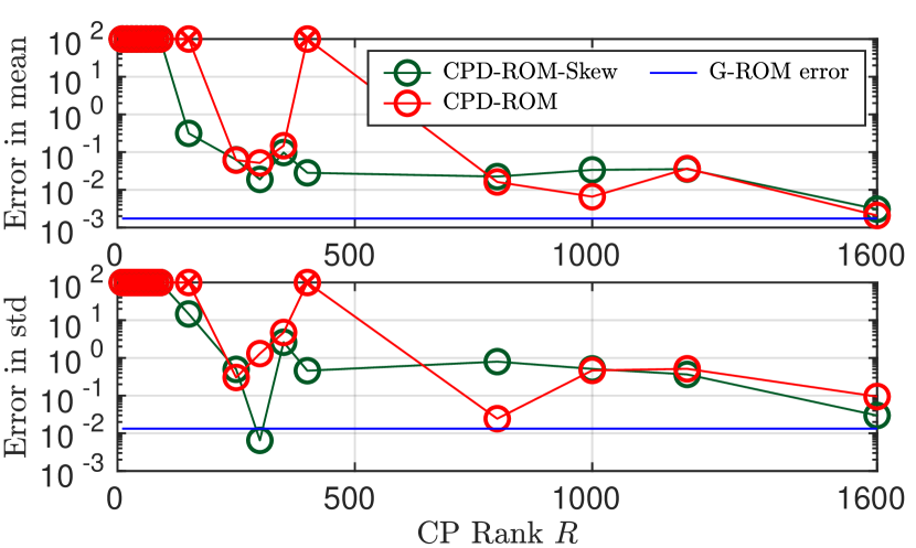
(a) $\rm Re=3200$

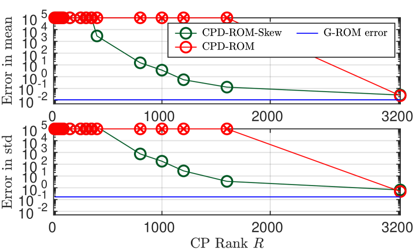
(b) $\rm Re=10000$

Figure 4.8: 3D lid-driven cavity: Comparison of the relative error in both the mean and the standard deviation of the energy between CPD-ROM-Skew and CPD-ROM as a function of the CP rank $R$ for (a) $\rm Re=3200$ and (b) $\rm Re=10,000$. The error is presented with respect to the FOM. The relative error of the G-ROM’s results with respect to the FOM is also illustrated as a blue dashed line. CPD-ROM-Skew is denoted as CPD-ROM with skew-symmetry preserved. The circle marker with a cross marker at several $R$ values, indicate solution blow-up, resulting in NaN errors.

Fig. 4.9 displays the results of the 3D MFU. In Figs. 9(a)–9(b), we compare the relative errors in the mean energy and its standard deviation between the CPD-ROM-Skew and the CPD-ROM as a function of CP rank $R$ for $\rm Re=3000$ and $\rm Re=5000$, respectively. The circle marker with a cross marker in the results of CPD-ROM, indicates solution blow-up, resulting in NaN errors. Again, we found CPD-ROM-Skew outperforms CPD-ROM for small $R$ values, and as $R$ increases, both behaves similarly. Moreover, higher Reynolds number requires larger $R$ for the CPD-ROM to be stable.

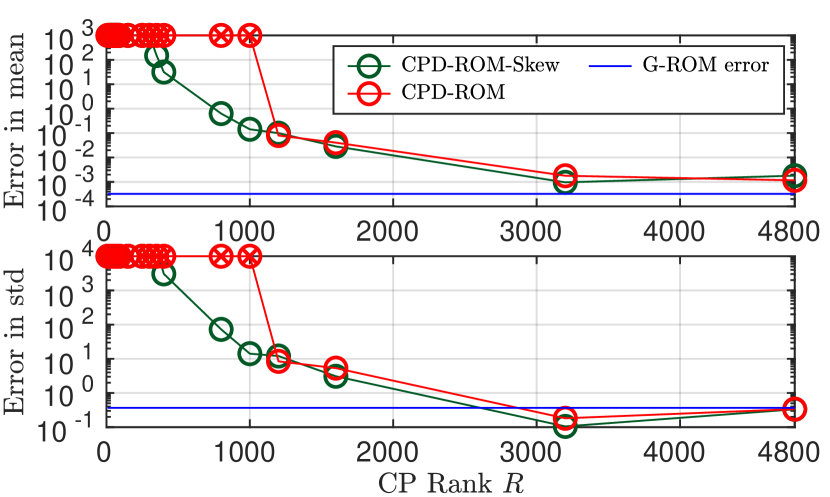
(a) $\rm Re=3000$

(b) $\rm Re=5000$

Figure 4.9: MFU: Comparison of the relative error in both the mean and the standard deviation of the energy between CPD-ROM-Skew and CPD-ROM as a function of the CP rank $R$ for (a) $\rm Re=3000$ and (b) $\rm Re=5000$. The error is presented with respect to the FOM. The relative error of the G-ROM’s results with respect to the FOM is also illustrated as a blue dashed line. CPD-ROM-Skew is denoted as CPD-ROM with skew-symmetry preserved. The circle marker with a cross marker at several $R$ values, indicate solution blow-up, resulting in NaN errors.

4.4 Numerical investigation of the G-ROM with the singular value decomposition (SVD)

In this section, we explore the use of the singular value decomposition (SVD) in the G-ROM as an alternative low-rank approximation for the tensor $\mathcal{C}$. In Section 4.4.1, we investigate the low-rank structure of the tensor using the SVD, specifically examining their behavior under the the $L^{2}$ and the $H^{1}_{0}$ norms. Additionally, we investigate the effectiveness of the low-rank approximation between the SVD and CPD by examining its relative residual in terms the compression ratio. Subsequently, in Section 4.4.2, we compare the performance of the SVD-ROM with the CPD-ROM.

4.4.1 Low-rank structure ablation

In the case of the SVD, we investigate the behavior of the singular values of $C_{(1)},~{}C_{(2)}$ and $C_{(3)}$, representing the mode-$1$, mode-$2$ and mode-$3$ matricized versions of the tensor $\mathcal{C}$. Note that each row of $C_{(3)}$ preserves the skew-symmetric property, unlike $C_{(1)}$ and $C_{(2)}$. For comparison purpose, we normalize the singular value with the first singular value.

In Fig. 4.10, the singular value behavior of $C_{(1)}$, $C_{(2)}$ and $C_{(3)}$ is presented with the POD basis using $L^{2}$ and $H^{1}_{0}$ norm, denoted as the $L^{2}$- and $H^{1}_{0}$-POD basis, respectively, in the 2D flow past a cylinder at $\rm Re=100$. We found the singular value of $C_{(3)}$ decays much faster compared to the results of $C_{(1)}$ and $C_{(2)}$ in both norm. This suggests there is a low-rank structure in $C_{(3)}$.

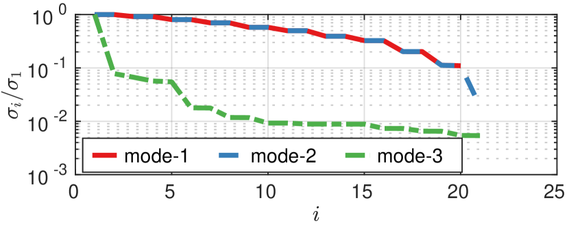
(a) $L^{2}$-POD basis

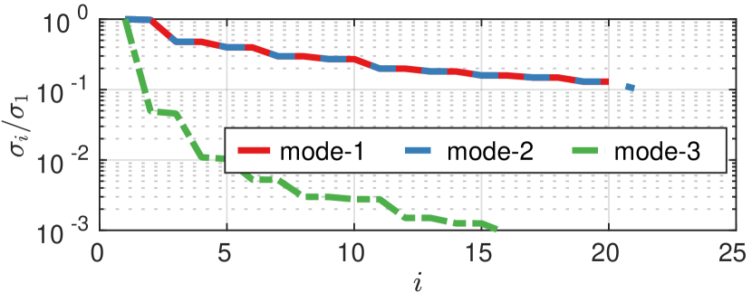
(b) $H^{1}_{0}$-POD basis

Figure 4.10: 2D flow past a cylinder at $\rm Re=100$: Singular value behavior of mode-1, mode-2, and mode-3 matricized version of $\mathcal{C}$ with (a) the $L^{2}$-POD basis and (b) the $H^{1}_{0}$-POD basis.

In addition, the singular value of all three matricized matrices decays much faster with the $H^{1}_{0}$ norm compared to the $L^{2}$ norm. As highlighted in [25], the $H^{1}_{0}$-POD basis is expected to perform better in capturing small-scale structures and distinguishing them from large-scale structures in the solution compared to the $L^{2}$-POD basis. Therefore, it is not surprising to find the singular value of all three matrices decay faster with the $H^{1}_{0}$ norm.

Fig. 4.11 shows the singular value behavior of $C_{(1)}$, $C_{(2)}$ and $C_{(3)}$ with $L^{2}$- and $H^{1}_{0}$-POD basis in the 2D lid-driven cavity at $\rm Re=15000$. We found the singular value of $C_{(1)}$ and $C_{(2)}$ behaves similarly regardless of the norm. For the singular value of $C_{(3)}$, we still found it decays much faster compared to the singular value of the other two matrices. However, the results with $H^{1}_{0}$ norm decays much faster compared to the $L^{2}$ norm. This indicates there is a low-rank structure in $C_{(3)}$ with $H^{1}_{0}$ but not $L^{2}$ norm.

Similar investigations were conducted for the tensors in the 3D lid-driven cavity and MFU, yielding consistent results with those observed in the 2D lid-driven cavity: the matrix $C_{(3)}$ exhibits a low-rank structure under the $H^{1}_{0}$ norm.

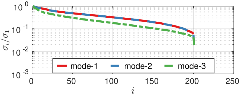
(a) $L^{2}$-POD basis

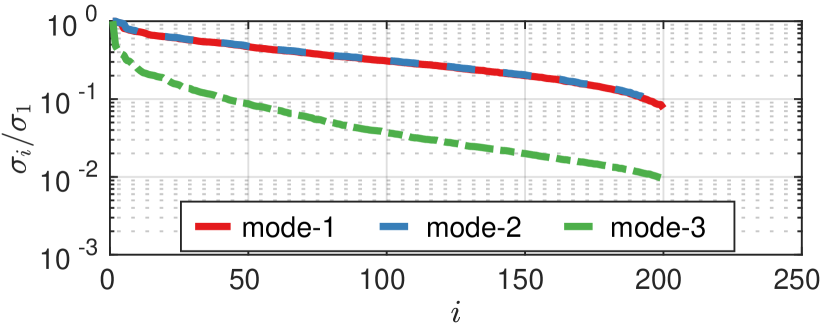
(b) $H^{1}_{0}$-POD basis

Figure 4.11: 2D lid-driven cavity at $\rm Re=15,000$: Singular value behavior of mode-1, mode-2, and mode-3 matricized version of $\mathcal{C}$ with (a) the $L^{2}$-POD basis and (b) the $H^{1}_{0}$-POD basis.

We further investigate the impact of the Reynolds number on the singular values’ behavior in the 3D lid-driven cavity and the MFU in Fig. 4.12 with a primary focus on the $H^{1}_{0}$-POD basis. Fig. 12(a) shows the singular value behavior of $C_{(1)}$ and $C_{(3)}$ in the 3D lid-driven cavity at $\rm Re=3200$ and $\rm Re=10,000$. We found the singular values of both $C_{(1)}$ and $C_{(3)}$ decay slightly faster in the case of higher Reynolds number. Fig. 12(b) shows the singular value behavior of $C_{(1)}$ and $C_{(3)}$ in the MFU at $\rm Re=3000$ and $\rm Re=5000$. Here we found a faster decay in the singular values of $C_{(1)}$ with the higher Reynolds number. Overall, our results do not reveal a significant difference in the singular values’ behavior between low and high Reynolds numbers.

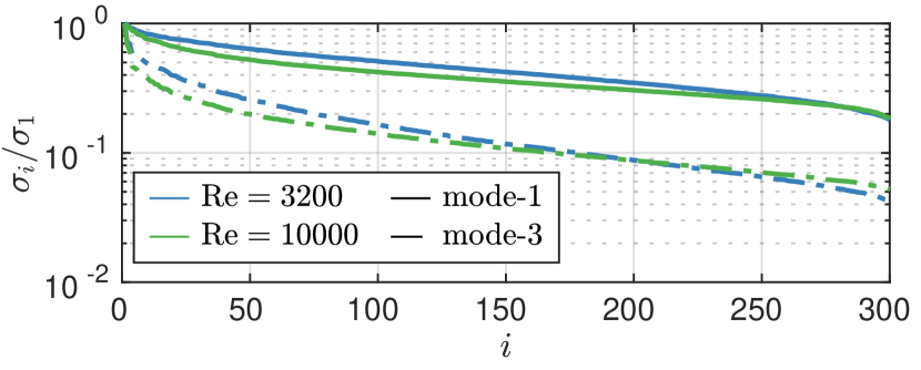
(a) 3D lid-driven cavity

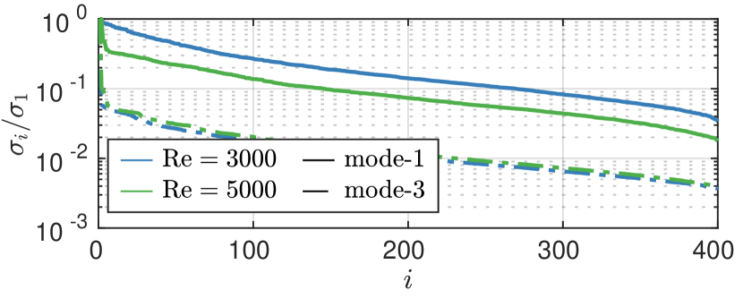
(b) Minimal flow unit

Figure 4.12: The effect of the Reynolds number on the singular value behavior of mode-1 and mode-3 matricized version of $\mathcal{C}$ with the $H^{1}_{0}$-POD basis in (a) the 3D lid-driven cavity and (b) the MFU with two Reynolds numbers presented in each case.

We next investigate the behavior of the relative residual as a function of the compression ratio (CR) to study the effectiveness of the SVD and the CPD for approximating the tensor $\mathcal{C}$. Given a tensor $\mathcal{C}$ and its approximated tensor ${\widehat{\mathcal{C}}}$, the relative residual is defined as:

$$r_{\text{rel}}:=\frac{\|\mathcal{C}-{\widehat{\mathcal{C}}}\|_{F}}{\|\mathcal{C}\|_{F}}.$$ (4.5)

For the SVD, the relative residual (4.5) is used to measure the approximation but with $C_{(3)}$ and $\widehat{C}_{(3)}$. In this study, we focus the CP decomposition with skew-symmetry preserved and the compression ratio for the ALS-skew and the SVD are defined as

$$\text{CR}_{ALS-Skew}=\frac{N^{3}}{\frac{3}{2}NR}=\frac{2N^{2}}{3R},\quad\text{CR}_{SVD}=\frac{N^{3}}{N^{2}R}=\frac{N}{R}.$$ (4.6)

Fig. 4.13 shows the behavior of the relative residual as a function of the CR for the SVD and the CPD in the 3D lid-driven cavity and the MFU. We found for a fixed relative residual, the CPD is much more effective compared to the SVD in terms of the compression ratio. Although the SVD is more robust in achieveing a smaller relative residual compared to the CPD, the CR is nearly $1$ and therefore use of the SVD achieves almost no speed-up. Moreover, based on our investigation in previous sections, a relative residual between $0.35$ to $0.1$ is sufficient for the CPD-ROM to perform comparably to the G-ROM.

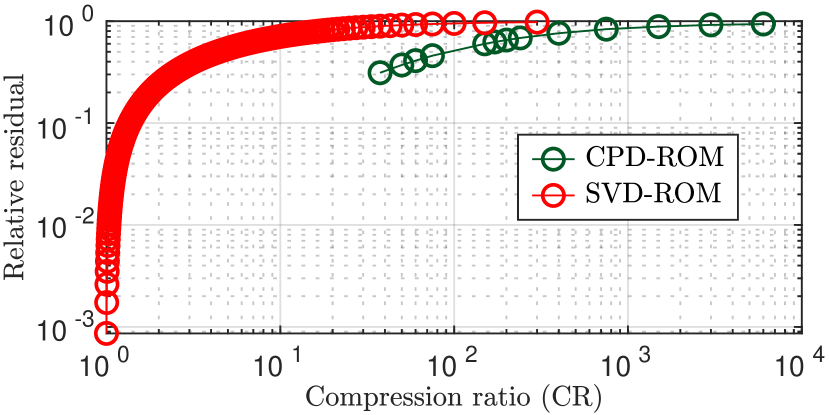
(a) 3D lid-driven cavity

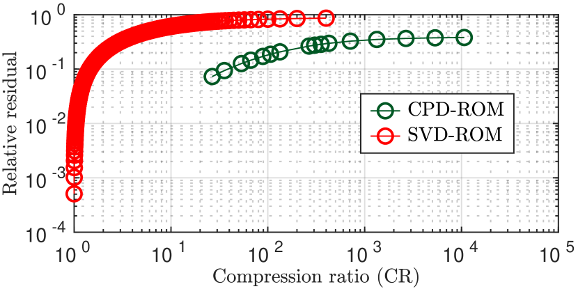
(b) MFU

Figure 4.13: The behavior of the relative residual of the approximated tensor with the SVD and the CPD as a function of the compression ratio (CR) in (a) the 3D lid-driven cavity and (b) the MFU. The compression ratio of the CPD and SVD are defined as $2N^{2}/R$ and $N/R$, respectively.

4.4.2 Performance investigation of the SVD-ROM with the CPD-ROM

In this section, we compare the performance of the SVD-ROM with the CPD-ROM. In the SVD-ROM, the tensor contraction $\mathcal{C}({\underline{u}}){\underline{u}}$ is evaluate using the approximated the mode-$3$ matricized version of the tensor $\mathcal{C}$:

$$C_{(3)}\approx\widehat{C}_{(3)}=U_{R}\Sigma_{R}V^{T}_{R},$$ (4.7)

where $U_{R}$ and $V_{R}$ are the left and right singular vector matrices of size $\mathbb{R}^{N\times R}$ and $\mathbb{R}^{N^{2}\times R}$, respectively. $\Sigma_{R}$ is the singular value matrix of size $\mathbb{R}^{R\times R}$.

In Figs. 4.14–4.15, the relative error in the mean and the standard deviation of the energy and energy of the fluctuated velocity is shown as a function of the compression ratio (CR) for the 3D lid-driven cavity and the MFU, respectively. In both the mean and the standard deviation, we found the CPD-ROM has a larger CR compared to the SVD-ROM for a given accuracy. This indicates CPD is more effective than the SVD.

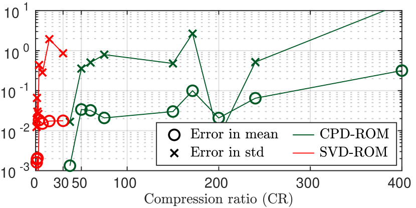
(a) Relative error in the mean energy and its standard deviation

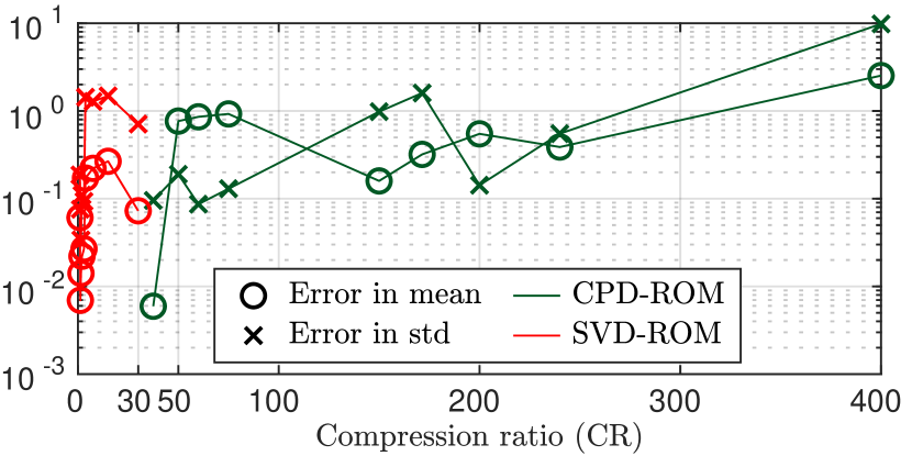
(b) Relative error in the mean $\mathrm{E}_{\text{fluc}}$ and its standard deviation

Figure 4.14: 3D lid-driven cavity at $\rm Re=3200$: Comparison of the relative error in both the mean and the standard deviation of (a) the energy and (b) the energy of the fluctuated velocity between the SVD-ROM and the CPD-ROM as a function of the compression ratio (CR) The compression ratio of the CPD and SVD are defined as $2N^{2}/R$ and $N/R$, respectively.

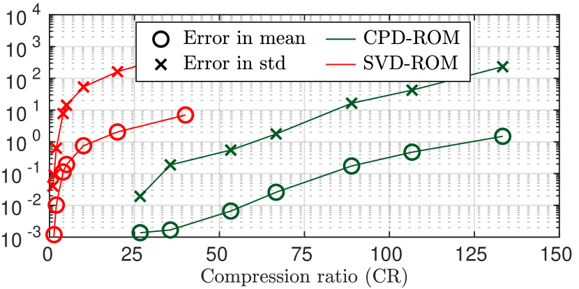
(a) Relative error in the mean energy and its standard deviation

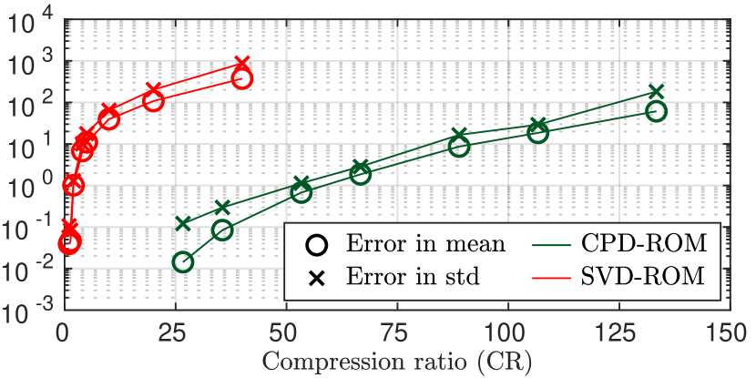
(b) Relative error in the mean $\mathrm{E}_{\text{fluc}}$ and its standard deviation

Figure 4.15: MFU at $\rm Re=5000$: Comparison of the relative error in both the mean and the standard deviation of (a) the energy and (b) the energy of the fluctuated velocity between the SVD-ROM and the CPD-ROM as a function of the compression ratio (CR) The compression ratio of the CPD and SVD are defined as $2N^{2}/R$ and $N/R$, respectively.

5 Conclusions and discussions

In this work, we propose a novel approach which utilizes the CANDECOMC/PARAFAC decomposition (CPD) to accelerate the G-ROM by approximating the reduced advection tensor by a sum of $R$ rank-1 tensors. From our numerical investigation in several 2D and 3D flow problems, we show that the G-ROM with the CP decomposition (CPD-ROM) is able to obtain at least a factor of $10$ speed-up. In addition, we show that skew-symmetry preserving CPD-ROM is more stable, and for a given accuracy allows a smaller CP rank $R$, which implies more speed-up. Moreover, we compare the CPD-ROM with the SVD-ROM, i.e., the G-ROM with the singular value decomposition (SVD). For a given accuracy, we show that CPD-ROM outperforms the SVD-ROM in terms of the compression ratio. Finally, from the singular value behavior, we show that the advection tensor with the $H^{1}_{0}$-POD basis has low-rank structure in its mode-$3$ matricized version.

The first step in the numerical investigation of the CPD-ROM has been encouraging. There are, however, several other research directions that should be pursued next. For example, the CP decomposition can also be applied to the energy equation which could further reduce the computational cost in the fluid-thermal applications. In addition, as we pointed out, for a general flow problem, the reduced tensor could be decomposed into a skew-symmetric part with a low-rank tensor contributed from the boundaries and it will be interesting to see how the CPD-ROM performs in this context. Moreover, in this work, we used the alternating least squares method (ALS) and its varianst to compute the CP decomposition. However, ALS may exhibit slow or no convergence, especially when high accuracy is required [69]. Therefore, it will be interesting to consider other optimization methods to construct the CPD-ROM and investigate if the resulting CPD-ROM is more accurate and is capable of achieving a larger speed-up. Finally, another possibility is to consider other tensor decompositions such as Tucker decomposition.

References

- [1] S. E. Ahmed, S. Pawar, O. San, A. Rasheed, T. Iliescu, and B. R. Noack. On closures for reduced order models A spectrum of first-principle to machine-learned avenues. Phys. Fluids, 33(9):091301, 2021.
- [2] Enrique Arrondo, Alessandra Bernardi, Pedro Macias Marques, and Bernard Mourrain. Skew-symmetric tensor decomposition. Communications in Contemporary Mathematics, 23(02):1950061, 2021.
- [3] Patricia Astrid, Siep Weiland, Karen Willcox, and Ton Backx. Missing point estimation in models described by proper orthogonal decomposition. IEEE Transactions on Automatic Control, 53(10):2237–2251, 2008.
- [4] Brett W Bader, Richard A Harshman, and Tamara G Kolda. Temporal analysis of semantic graphs using ASALSAN. In Seventh IEEE international conference on data mining (ICDM 2007), pages 33–42. IEEE, 2007.
- [5] F. Ballarin, A. Manzoni, A. Quarteroni, and G. Rozza. Supremizer stabilization of POD–Galerkin approximation of parametrized steady incompressible Navier–Stokes equations. Int. J. Numer. Meth. Engng., 102:1136–1161, 2015.
- [6] Maxime Barrault, Yvon Maday, Ngoc Cuong Nguyen, and Anthony T Patera. An empirical interpolation method: Application to efficient reduced-basis discretization of partial differential equations. Comptes Rendus Mathematique, 339(9):667–672, 2004.
- [7] Erna Begovic and Lana Perisa. CP decomposition and low-rank approximation of antisymmetric tensors. arXiv preprint arXiv:2212.13389, 2022.
- [8] Gal Berkooz, Philip Holmes, and John L Lumley. The proper orthogonal decomposition in the analysis of turbulent flows. Annual review of fluid mechanics, 25(1):539–575, 1993.
- [9] S. L. Brunton and J. N. Kutz. Data-driven science and engineering: Machine learning, dynamical systems, and control. Cambridge University Press, 2019.
- [10] Kevin Carlberg, Charbel Farhat, Julien Cortial, and David Amsallem. The GNAT method for nonlinear model reduction: effective implementation and application to computational fluid dynamics and turbulent flows. Journal of Computational Physics, 242:623–647, 2013.
- [11] J Douglas Carroll and Jih-Jie Chang. Analysis of individual differences in multidimensional scaling via an N-way generalization of “Eckart-Young” decomposition. Psychometrika, 35(3):283–319, 1970.
- [12] Saifon Chaturantabut and Danny C Sorensen. Discrete empirical interpolation for nonlinear model reduction. In Proceedings of the 48h IEEE Conference on Decision and Control (CDC) held jointly with 2009 28th Chinese Control Conference, pages 4316–4321. IEEE, 2009.
- [13] Saifon Chaturantabut and Danny C Sorensen. Nonlinear model reduction via discrete empirical interpolation. SIAM Journal on Scientific Computing, 32(5):2737–2764, 2010.
- [14] Saifon Chaturantabut and Danny C Sorensen. Application of POD and DEIM on dimension reduction of non-linear miscible viscous fingering in porous media. Mathematical and Computer Modelling of Dynamical Systems, 17(4):337–353, 2011.
- [15] Alexander V Chikitkin, Egor K Kornev, and Vladimir A Titarev. Numerical solution of the Boltzmann equation with S-model collision integral using tensor decompositions. Computer Physics Communications, 264:107954, 2021.
- [16] Youngsoo Choi and Kevin Carlberg. Space–time least-squares Petrov–Galerkin projection for nonlinear model reduction. SIAM Journal on Scientific Computing, 41(1):A26–A58, 2019.
- [17] Pierre Comon, Gene Golub, Lek-Heng Lim, and Bernard Mourrain. Symmetric tensors and symmetric tensor rank. SIAM Journal on Matrix Analysis and Applications, 30(3):1254–1279, 2008.
- [18] Lieven De Lathauwer, Bart De Moor, and Joos Vandewalle. A multilinear singular value decomposition. SIAM journal on Matrix Analysis and Applications, 21(4):1253–1278, 2000.
- [19] V. DeCaria, T. Iliescu, W. Layton, M. McLaughlin, and M. Schneier. An artificial compression reduced order model. SIAM J. Numer. Anal., 58(1):565–589, 2020.
- [20] Ke Ding. Free response of a freely-rotatable eccentric linearly-sprung circular cylinder in or absent a cross-flow. PhD thesis, 2021.
- [21] Sergey Dolgov and Martin Stoll. Low-rank solution to an optimization problem constrained by the Navier–Stokes equations. SIAM Journal on Scientific Computing, 39(1):A255–A280, 2017.
- [22] Carl Eckart and Gale Young. The approximation of one matrix by another of lower rank. Psychometrika, 1(3):211–218, 1936.
- [23] Lukas Einkemmer, Alexander Ostermann, and Chiara Piazzola. A low-rank projector-splitting integrator for the Vlasov–Maxwell equations with divergence correction. Journal of Computational Physics, 403:109063, 2020.
- [24] Howard C Elman and Virginia Forstall. Numerical solution of the parameterized steady-state Navier–Stokes equations using empirical interpolation methods. Computer Methods in Applied Mechanics and Engineering, 317:380–399, 2017.
- [25] Lambert Fick, Yvon Maday, Anthony T Patera, and Tommaso Taddei. A stabilized POD model for turbulent flows over a range of Reynolds numbers: Optimal parameter sampling and constrained projection. Journal of Computational Physics, 371:214–243, 2018.
- [26] P. Fischer, M. Schmitt, and A. Tomboulides. Recent developments in spectral element simulations of moving-domain problems, volume 79, pages 213–244. Fields Institute Communications, Springer, 2017.
- [27] Paul Fischer, Stefan Kerkemeier, Misun Min, Yu-Hsiang Lan, Malachi Phillips, Thilina Rathnayake, Elia Merzari, Ananias Tomboulides, Ali Karakus, Noel Chalmers, et al. NekRS, a GPU-accelerated spectral element Navier–Stokes solver. Parallel Computing, 114:102982, 2022.
- [28] Paul Fischer, Martin Schmitt, and Ananias Tomboulides. Recent developments in spectral element simulations of moving-domain problems. In Recent Progress and Modern Challenges in Applied Mathematics, Modeling and Computational Science, pages 213–244. Springer, 2017.
- [29] Paul F Fischer, James W Lottes, and Stefan G Kerkemeier. Nek5000 web page, 2008.
- [30] Douglas G Fox and Steven A Orszag. Pseudospectral approximation to two-dimensional turbulence. Journal of Computational Physics, 11(4):612–619, 1973.
- [31] Wei Guo and Jing-Mei Qiu. A low rank tensor representation of linear transport and nonlinear Vlasov solutions and their associated flow maps. Journal of Computational Physics, 458:111089, 2022.
- [32] RA Harshman and ME Lundy. Three-way DEDICOM: Analyzing multiple matrices of asymmetric relationships. In Annual Meeting of the North American Psychometric Society, 1992.
- [33] Richard A Harshman. Models for analysis of asymmetrical relationships among N objects or stimuli. In Paper presented at the First Joint Meeting of the Psychometric Society and the Society of Mathematical Psychology, Hamilton, 1978.
- [34] Richard A Harshman et al. Foundations of the PARAFAC procedure: Models and conditions for an” explanatory” multimodal factor analysis. 1970.
- [35] Johan Håstad. Tensor rank is NP-complete. Journal of Algorithms, 11(4):644–654, 1990.
- [36] J. S. Hesthaven, G. Rozza, and B. Stamm. Certified Reduced Basis Methods for Parametrized Partial Differential Equations. Springer, 2015.
- [37] Christopher J Hillar and Lek-Heng Lim. Most tensor problems are np-hard. Journal of the ACM (JACM), 60(6):1–39, 2013.
- [38] Frank L Hitchcock. The expression of a tensor or a polyadic as a sum of products. Journal of Mathematics and Physics, 6(1-4):164–189, 1927.
- [39] Felix Hummel, Theodoros Tsatsoulis, and Andreas Grüneis. Low rank factorization of the Coulomb integrals for periodic coupled cluster theory. The Journal of chemical physics, 146(12):124105, 2017.
- [40] Edwin Insuasty, Paul MJ Van den Hof, Siep Weiland, and Jan Dirk Jansen. Tensor-based reduced order modeling in reservoir engineering: An application to production optimization. IFAC-PapersOnLine, 48(6):254–259, 2015.
- [41] Yakov Itin and Shulamit Reches. Decomposition of third-order constitutive tensors. Mathematics and Mechanics of Solids, 27(2):222–249, 2022.
- [42] Javier Jiménez and Parviz Moin. The minimal flow unit in near-wall turbulence. Journal of Fluid Mechanics, 225:213–240, 1991.
- [43] Muneaki Kamiya and So Hirata. Higher-order equation-of-motion coupled-cluster methods for electron attachment. The Journal of chemical physics, 126(13), 2007.
- [44] Kento Kaneko. An augmented basis method for reduced order models of turbulent flow. PhD thesis, 2022.
- [45] Kento Kaneko, Ping-Hsuan Tsai, and Paul Fischer. Towards model order reduction for fluid-thermal analysis. Nuclear Engineering and Design, 370:110866, 2020.
- [46] John Kim, Parviz Moin, and Robert Moser. Turbulence statistics in fully developed channel flow at low Reynolds number. Journal of fluid mechanics, 177:133–166, 1987.
- [47] Othmar Koch and Christian Lubich. Dynamical tensor approximation. SIAM Journal on Matrix Analysis and Applications, 31(5):2360–2375, 2010.
- [48] Tamara G Kolda. Numerical optimization for symmetric tensor decomposition. Mathematical Programming, 151(1):225–248, 2015.
- [49] Tamara G Kolda and Brett W Bader. Tensor decompositions and applications. SIAM review, 51(3):455–500, 2009.
- [50] Tamara Gibson Kolda. Multilinear operators for higher-order decompositions. Technical report, Sandia National Laboratories, 2006.
- [51] Erna Begovic Kovac and Daniel Kressner. Structure-preserving low multilinear rank approximation of antisymmetric tensors. SIAM Journal on Matrix Analysis and Applications, 38(3):967–983, 2017.
- [52] Joseph B Kruskal. Three-way arrays: rank and uniqueness of trilinear decompositions, with application to arithmetic complexity and statistics. Linear algebra and its applications, 18(2):95–138, 1977.
- [53] Yu-Hsiang Lan. On the development of preconditioning the advection diffusion operators with spectral element discretization. PhD thesis, University of Illinois at Urbana-Champaign, 2023.
- [54] Per-Olov Löwdin. Quantum theory of many-particle systems. II. Study of the ordinary Hartree-Fock approximation. Physical Review, 97(6):1490, 1955.
- [55] Margaret E Lundy, Richard A Harshman, Pentti Paatero, and Leora C Swartzman. Application of the 3-way Dedicom model to skew-symmetric data for paired preference ratings of treatments for chronic back pain. In TRICAP 2003 Meeting, Lexington, Kentucky. Citeseer, 2003.
- [56] P Lykos and GW Pratt. Discussion on the Hartree-Fock approximation. Reviews of Modern Physics, 35(3):496, 1963.
- [57] Yvon Maday, Anthony T Patera, and Einar M Ronquist. A well-posed optimal spectral element approximation for the Stokes problem. Technical report, 1987.
- [58] Johan Malm, Philipp Schlatter, Paul F Fischer, and Dan S Henningson. Stabilization of the spectral element method in convection dominated flows by recovery of skew-symmetry. Journal of Scientific Computing, 57:254–277, 2013.
- [59] Robert D Moser, John Kim, and Nagi N Mansour. Direct numerical simulation of turbulent channel flow up to = 590. Physics of fluids, 11(4):943–945, 1999.
- [60] B. R. Noack, M. Morzynski, and G. Tadmor. Reduced-Order Modelling for Flow Control, volume 528. Springer Verlag, 2011.
- [61] B. R. Noack, P. Papas, and P. A. Monkewitz. The need for a pressure-term representation in empirical Galerkin models of incompressible shear flows. J. Fluid Mech., 523:339–365, 2005.
- [62] Achim Nonnenmacher and Christian Lubich. Dynamical low-rank approximation: Applications and numerical experiments. Mathematics and Computers in Simulation, 79(4):1346–1357, 2008.
- [63] Steven A Orszag. Comparison of pseudospectral and spectral approximation. Studies in Applied Mathematics, 51(3):253–259, 1972.
- [64] Steven A Orszag and Moshe Israeli. Numerical simulation of viscous incompressible flows. Annual Review of Fluid Mechanics, 6(1):281–318, 1974.
- [65] Bérengère Podvin and John Lumley. A low-dimensional approach for the minimal flow unit. Journal of Fluid Mechanics, 362:121–155, 1998.
- [66] George D Purvis III and Rodney J Bartlett. A full coupled-cluster singles and doubles model: The inclusion of disconnected triples. The Journal of Chemical Physics, 76(4):1910–1918, 1982.
- [67] A. Quarteroni, A. Manzoni, and F. Negri. Reduced Basis Methods for Partial Differential Equations: An Introduction, volume 92. Springer, 2015.
- [68] Yukiko S Shimizu and Eric J Parish. Windowed space–time least-squares Petrov–Galerkin model order reduction for nonlinear dynamical systems. Computer Methods in Applied Mechanics and Engineering, 386:114050, 2021.
- [69] Navjot Singh, Linjian Ma, Hongru Yang, and Edgar Solomonik. Comparison of accuracy and scalability of Gauss–Newton and alternating least squares for CANDECOMC/PARAFAC decomposition. SIAM Journal on Scientific Computing, 43(4):C290–C311, 2021.
- [70] Edgar Solomonik, Devin Matthews, Jeff R Hammond, John F Stanton, and James Demmel. A massively parallel tensor contraction framework for coupled-cluster computations. Journal of Parallel and Distributed Computing, 74(12):3176–3190, 2014.
- [71] Yifei Sun and Mrinal Kumar. Numerical solution of high dimensional stationary Fokker–Planck equations via tensor decomposition and Chebyshev spectral differentiation. Computers & Mathematics with Applications, 67(10):1960–1977, 2014.
- [72] Szilárd Szalay, Max Pfeffer, Valentin Murg, Gergely Barcza, Frank Verstraete, Reinhold Schneider, and Örs Legeza. Tensor product methods and entanglement optimization for ab initio quantum chemistry. International Journal of Quantum Chemistry, 115(19):1342–1391, 2015.
- [73] Richard F Tinder. Tensor properties of solids: phenomenological development of the tensor properties of crystals, volume 4. Morgan & Claypool Publishers, 2008.
- [74] Ping-Hsuan Tsai. Parametric Model Order Reduction Development for Navier-Stokes Equations from 2D Chaotic to 3D Turbulent Flow Problems. PhD thesis, 2023.
- [75] Ping-Hsuan Tsai and Paul Fischer. Parametric model-order-reduction development for unsteady convection. Frontiers in Physics, 10:903169, 2022.
- [76] S. Volkwein. Proper orthogonal decomposition: Theory and reduced-order modelling. Lecture Notes, University of Konstanz, 2013. http://www.math.uni-konstanz.de/numerik/personen/volkwein/teaching/POD-Book.pdf.
- [77] Dunhui Xiao, Fangxin Fang, Andrew G Buchan, Christopher C Pain, Ionel Michael Navon, Juan Du, and G Hu. Non-linear model reduction for the Navier–Stokes equations using residual DEIM method. Journal of Computational Physics, 263:1–18, 2014.