Abstract

Discriminatively trained, deterministic neural networks are the de facto choice for classification problems. However, even though they achieve state-of-the-art results on in-domain test sets, they tend to be overconfident on out-of-distribution (OOD) data. For instance, ReLU networks—a popular class of neural network architectures—have been shown to almost always yield high confidence predictions when the test data are far away from the training set, even when they are trained with OOD data. We overcome this problem by adding a term to the output of the neural network that corresponds to the logit of an extra class, that we design to dominate the logits of the original classes as we move away from the training data. This technique provably prevents arbitrarily high confidence on far-away test data while maintaining a simple discriminative point-estimate training. Evaluation on various benchmarks demonstrates strong performance against competitive baselines on both far-away and realistic OOD data.

1 Introduction

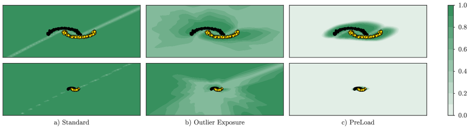
Figure 1: An illustrative example of the confidence of different methods trained on a synthetic binary classification dataset. The shades of green display the confidence of each algorithm with a darker shade signifying a higher confidence. The bottom row gives a zoomed-out view.

Machine learning has made substantial progress over the last decade with the help of a strong deep learning toolkit, larger data sets, better optimization algorithms, faster and cheaper computation, and a vibrant research community. As machine learning systems continue to be deployed in safety-critical applications, important questions around their robustness and uncertainty quantification continue to be asked. A common expectation in uncertainty quantification is to assign high confidence to test cases close to the training data and low confidence to test cases that are out-of-distribution (OOD).

Recent advances in machine learning are in part due to deep neural networks (DNNs), which are powerful function approximators. However, DNN classifiers tend to be overconfident for both in-domain examples (Guo et al., 2017) and data that is far away from the training examples (Nguyen et al., 2015). Hein et al. (2019) showed that the ubiquitous ReLU Networks almost always exhibit high confidence on samples that are far away from the training data.

A number of methods have been proposed to deal with the overconfidence issue in DNNs. Calibration methods attempt to solve overconfidence of neural network classifiers by various methods including smoothing the softmax distribution (Guo et al., 2017; Gupta et al., 2020; Kull et al., 2019), regularization (Müller et al., 2019; Thulasidasan et al., 2019) and adding additional constraints to the loss function (Kumar et al., 2018; Lin et al., 2017). These methods, however, do not resolve overconfidence issues around OOD data (Minderer et al., 2021). Other methods, both Bayesian (Blundell et al., 2015; Gal and Ghahramani, 2016; Kristiadi et al., 2020) and non-Bayesian (Lakshminarayanan et al., 2017; Mukhoti et al., 2023) have improved OOD detection while training only the in-domain data distribution.

State-of-the-art methods for OOD detection are typically trained with additional OOD training data with the goal for the classifier to output either high “None” class probability (Zhang and LeCun, 2017; Kristiadi et al., 2022a) or uniform confidence (Hendrycks et al., 2018), in the presence of OOD samples. Hein et al. (2019) showed that there is no guarantee that OOD data would go to the “None” class. Moreover, these methods still exhibit high confidence when the test points are far away from the data.

One way of overcoming the problem of arbitrarily high confidence on far-away data is to incorporate generative modeling, either as a posthoc method (Lee et al., 2018; Mukhoti et al., 2023) or as a prior on the data (Meinke and Hein, 2020), into a neural network. The former assumes that the neural network embedding can be approximated with a Gaussian distribution. However, on realistic, ‘near’ OOD data, we will demonstrate that these methods are not competitive with the state-of-the-art. The latter assumes a generative model over the data which is a harder problem than the underlying discriminative modeling.

Finally, while Bayesian neural networks (Louizos and Welling, ; Kristiadi et al., 2022b) have also been used to overcome this issue, they are not guaranteed to obtain the optimal confidences on far-away OOD test data (Kristiadi et al., 2020). While a more sophisticated remedy exists for this (Kristiadi et al., 2021), they are specifically constructed to only fix the far-away high confidence, and their detection performance on ‘nearby‘ OOD data are more of an afterthought.

In this work, we present our method, called Producing Larger Logits away from Data, or PreLoad, which fulfills the following desiderata: (i) it must maintain the simplicity of the standard discriminative training procedure for DNNs (unlike generative- and Bayesian-based methods), (ii) it must provably be less confident on inputs far away from the training data, and (iii) it must perform well on realistic OOD examples (e.g. CIFAR-10 vs. CIFAR-100).

We accomplish this by training an extra class, such that under an OOD input, this extra logit is larger than the logits of the other classes as we move farther away from the training data. This construction provably helps PreLoad almost always predict far-away data as OOD. Furthermore, the extra class is trained on an auxiliary, OOD dataset, which helps it detect realistic, nearby OOD examples well.

Figure 1 illustrates the confidence level of PreLoad as we move away from the training data, compared to a standard-trained neural network and a discriminative OOD training approach called Outlier Exposure (OE, Hendrycks et al., 2018). Standard neural networks with a softmax output layer exhibit high confidence as we move away from the decision boundary. OE’s confidence initially decreases away from the data, but it becomes high far away as we zoom out. In contrast, PreLoad is confident when close to the data and uncertain when away from it.

2 Preliminaries

We define a neural network as a function $f:\mathbb{R}^{n}\times\mathbb{R}^{p}\to\mathbb{R}^{k}$ with $(x,\theta)\mapsto f_{\theta}(x)$, where $\mathbb{R}^{n}$ is the input space, $\mathbb{R}^{k}$ the output space, and $\mathbb{R}^{p}$ the parameter space. Let $\mathcal{D}:=\{(x_{i},y_{i})\}_{i=1}^{m}$ be a training dataset. The standard way of training a neural network is by finding optimal parameters $\theta^{*}$ such that $\theta^{*}=\operatorname*{arg\,min}_{\theta}\sum_{i=1}^{m}\ell(f_{\theta}(x_{i}),y_{i})$ for some loss function $\ell$ such as the cross-entropy loss for classification.

One of the most widely used neural network architectures is a ReLU network. We use the term ReLU networks for feedforward neural networks with piecewise affine activation functions, such as the ReLU or leaky ReLU activation, and a linear output layer. ReLU networks can be written as continuous piecewise affine functions (Arora et al., 2018; Hein et al., 2019).

Definition 1.

A function $f:\mathbb{R}^{n}\to\mathbb{R}$ is called piecewise affine if there exists a set of polytopes $\{Q_{r}\}_{r=1}^{M}$ such that their union is $\mathbb{R}^{n}$ and $f$ is affine in each polytope (Arora et al., 2018; Hein et al., 2019).

Piecewise affine functions include networks with fully connected layers, convolution layers, residual layers, skip connections, average pooling, and max pooling. We will rely on the neural network being a continuous piecewise affine function to prove that our algorithm prevents arbitrarily high confidence on far-away data.

Consider a classification problem where $x$ is the input and $y\in\{1,\cdots,k\}$ denotes the target class. A neural network with a linear output layer in conjunction with the softmax link function can be used to compute the probability $P(y|x)$. More precisely, consider the following decomposition of the neural network $f_{\theta}(x)=WG_{\psi}(x)$ where $W\in\mathbb{R}^{k\times d}$ is the weight matrix for the last layer, $G_{\psi}(x)\in\mathbb{R}^{d}$ is the neural network embedding and $\theta=\{\psi,W\}$. Each row of $f$ corresponds to the logit $z_{c}(x)$ of class $c$:

$$z_{c}(x)=w_{c}^{\top}G_{\psi}(x)+b_{c}.$$ (1)

Then the last layer computes class probabilities via a softmax such that:

$$P(y=c|x)=\frac{\exp(w^{\top}_{c}G_{\psi}(x)+b_{c})}{\sum_{c^{\prime}}\exp(w^{\top}_{c^{\prime}}G_{\psi}(x)+b_{c^{\prime}})}$$ (2)

where $w_{c}\in\mathbb{R}^{d}$ and $b_{c}\in\mathbb{R}$ are the parameters of the last layer associated with class $c\in\{1,\cdots,k\}$.

Generally, learning $P(y|x)$ is referred to as discriminative modeling. Generative models, such as GANs (Goodfellow et al., 2014) and VAEs (Kingma and Welling, 2013) learn the distribution of the data $P(x)$. Meanwhile, class-conditional generative models (Mukhoti et al., 2023) learn $P(x|y)$.

2.1 Arbitrarily High Confidence on Far-Away Data

Arbitrarily high confidence on far-away data i.e. data which is far away from the training set (Hein et al., 2019), can be formalized as observing that the probability of some class approaches $1$ in the limit of moving infinitely far from the training data.

Definition 2.

A model exhibits far-away arbitrarily high confidence if there exists $x\in\mathbb{R}^{n}$ and $c\in\{1,\cdots,k\}$ such that

$$\lim_{t\rightarrow\infty}P(y=c|tx)=1.$$ (3)

Hein et al. (2019) showed that piecewise affine networks (including ReLU networks) with a linear last layer almost always exhibit arbitrarily high confidence far away from the training data.

3 Methodology

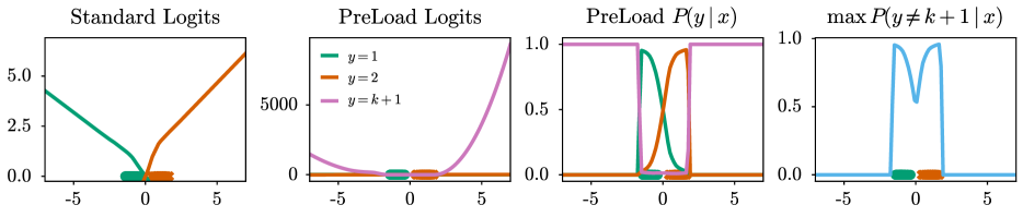
Figure 2: Effect of training with an OOD class with our method on a $1$-D binary classification problem. Standard logits keep on growing when away from the data. We implement the OOD class such that the logits grow much faster for the OOD class compared to the in-domain class. This ‘fixes’ the probabilities and the confidence away from the dataset. Note that the range of y values is larger on the second plot.

Consider a neural network, $f_{\psi,W}$ , trained on a $k$-class classification problem such that the logit $z_{c}$ is defined according to (1) and $P(y|x)$ is computed according to (2). Arbitrarily high confidence arises when the logit of one class becomes infinitely higher than the logits of the other classes:

Lemma 3.

Let $P(y|x)$ be a classifier defined in (2) and let $x\in\mathbb{R}^{n}$. If arbitrarily high confidence (i.e., $\lim_{t\rightarrow\infty}P(y|tx)=1$), then there must exist $c\in\{1,\dots,k\}$ such that $\lim_{t\rightarrow\infty}z_{c}(tx)-z_{c^{\prime}}(tx)=+\infty$ for all $c^{\prime}\neq c$.

Proof.

From (2), if $\lim_{t\rightarrow\infty}P(y=c|tx)=1$, we have:

$$\lim_{t\rightarrow\infty}\frac{\exp(z_{c}(tx))}{\sum_{c^{\prime}}\exp(z_{c^{\prime}}(tx))}=1.$$

Therefore,

$$\lim_{t\rightarrow\infty}\frac{\exp(z_{c}(tx))}{\sum_{c^{\prime}}\exp(z_{c^{\prime}}(tx))}=1$$

$$\implies \lim_{t\rightarrow\infty}\frac{\sum_{c^{\prime}}\exp(z_{c^{\prime}}(tx))}{\exp(z_{c}(tx))}=1$$

$$\implies \lim_{t\rightarrow\infty}1+\sum_{c^{\prime}\neq c}\frac{\exp(z_{c^{\prime}}(tx))}{\exp(z_{c}(tx))}=1$$

$$\implies \lim_{t\rightarrow\infty}\sum_{c^{\prime}\neq c}\exp(z_{c^{\prime}}(tx)-z_{c}(tx))=0$$

$$\implies \lim_{t\rightarrow\infty}\exp(z_{c^{\prime}}(tx)-z_{c}(tx))=0\quad\forall c^{\prime}\neq c.$$

Thus, we can conclude that $\lim_{t\rightarrow\infty}z_{c}(tx)-z_{c^{\prime}}(tx)=+\infty$ for all $c^{\prime}\neq c$. ∎

An immediate consequence of the above lemma is that networks with normalization such as layernorm do not suffer from far-away arbitrarily high confidence since the layers that follow layernorm (including the logits) will remain bounded. Note that networks with batchnorm may still exhibit far-away arbitrarily high confidence since batchnorm ensures that the logits of the training set are bounded, but not necessarily the logits of the test set, which may include OOD data that could be arbitrarily far.

Our solution consists of creating an additional, $(k+1)$-st class such that the confidence in the original classes vanishes far away from the training data while the confidence in the $(k+1)$-st class becomes arbitrarily high. Note that this is desirable since the extra class represents the OOD class. Based on lemma 3, we achieve this by making sure that the corresponding logit $z_{k+1}$ is infinitely higher than the logits $z_{c\in\{1,...,k\}}$ of the other classes far away from the training data. More precisely, let

$$z_{k+1}(x)=w_{k+1}^{\top}G_{\psi}(x)^{2}+b_{k+1}$$ (4)

where the weights $w_{k+1}\in\mathbb{R}^{d}_{>0}$ are restricted within the positive orthant and $G_{\psi}(x)^{2}$ is the component-wise square of the network embedding $G_{\psi}(x)$.

Then, given these logits, classification is performed as follows:

$$P(y=c|x)=\frac{1}{A(x)}\exp(w_{c}^{\top}G_{\psi}(x)+b_{c})$$ (5)

for $c\in\{1,\dots,k\}$, and

$$P(y=k+1|x)=\frac{1}{A(x)}\exp(w_{k+1}^{\top}G_{\psi}(x)^{2}+b_{k+1}),$$ (6)

where

$$A(x):=\sum_{c^{\prime}} \exp(w_{c^{\prime}}^{\top}G_{\psi}(x)+b_{c^{\prime}})$$ (7)

$$+\exp(w_{k+1}^{\top}G_{\psi}(x)^{2}+b_{k+1})$$

is the softmax’s denominator.

Intuitively, as we move away from the training data the magnitude of $G_{\psi}(x)$ may also increase, which may result in some class $c$ dominating with arbitrarily high confidence (Hein et al., 2019). However, by using $G_{\psi}(x)^{2}$ in the logit of the $(k+1)$-st class we make sure that it grows faster than other logits and therefore, eventually dominates. In Theorem 4, we prove that any classification network augmented with such a construction never exhibits far-away arbitrarily high confidence in classes $\{1,...,k\}$.

Theorem 4.

Let $G_{\psi}$ be any neural network embedding used for classification according to (5) and (6). Let $w_{c}$ and $b_{c}$ be finite weights and biases in the penultimate classification layer for each class $c$. Let $tx_{*}\in\mathbb{R}^{n}$ be a test input with magnitude regulated by $t$. Then $\lim_{t\rightarrow\infty}P(y=c|tx_{*})<1$ for all $c\neq k+1$.

Proof.

Based on lemma 3, arbitrarily high confidence (i.e., $\lim_{t\rightarrow\infty}P(y=c|tx)=1$) arises when there is a $c$ such that $\lim_{t\rightarrow\infty}z_{c}(tx)-z_{c^{\prime}}(tx)=\infty$ $\forall c^{\prime}\neq c$. We prove by contradiction that this cannot happen once we introduce the extra class with its logit as defined in (4). Consider two cases:

1. Suppose that there exists a class $c\neq k+1$ such that $\lim_{t\rightarrow\infty}z_{c}(tx)=\infty$ and for all $c^{\prime}\neq c$, $\lim_{t\rightarrow\infty}z_{c}(tx)-z_{c^{\prime}}(tx)=\infty$. Since $z_{c}(tx)=w_{c}^{\top}G_{\psi}(x)+b_{c}$, and the weights and biases are finite, then $\lim_{t\rightarrow\infty}z_{c}(tx)=\infty$ implies that $\lim_{t\rightarrow\infty}\|G_{\psi}(tx)\|=\infty$. Since $z_{k+1}(tx)=w_{k+1}^{\top}(G_{\psi}(x)^{2})+b_{k+1}$ where $w_{k+1}\in\mathbb{R}^{d}_{>0}$, i.e. each component of $w_{k+1}$ is positive, and that $G_{\psi}(x)^{2}$ is always component-wise positive, then $\lim_{t\rightarrow\infty}z_{k+1}(tx)=\infty$ and $\lim_{t\rightarrow\infty}z_{k+1}(tx)>\lim_{t\rightarrow\infty}z_{c}(tx)$, which contradicts the assumption that $\lim_{t\rightarrow\infty}z_{c}(tx)-z_{k+1}(tx)=\infty$.

2. Suppose that there exists a class $c\neq k+1$ such that $\lim_{t\rightarrow\infty}z_{c}(tx)<\infty$ and for all $c^{\prime}\neq c$, $\lim_{t\rightarrow\infty}z_{c}(tx)-z_{c^{\prime}}(tx)=\infty$. Since $z_{k+1}=w_{k+1}^{\top}(G_{\psi}(x)^{2})+b_{k+1}$, $w_{k+1}\in\mathbb{R}^{d}_{>0}$, $G_{\psi}(x)^{2}>0$ and $b_{k+1}<\infty$, then $\lim_{t\rightarrow\infty}z_{k+1}(tx)>-\infty$, which contradicts the assumption that $\lim_{t\rightarrow\infty}z_{c}(tx)-z_{k+1}(tx)=\infty$.

Altogether, they imply the desired result. ∎

The above theorem guarantees that arbitrarily high confidence will not occur for any neural network with an extra class that we propose. In addition, we show a stronger result in Theorem 6 for ReLU classification networks. As we move far away from the training data, we show that the confidence in the original classes (i.e., $c\in\{1,...,k\}$) will be dominated by the extra class. To prove this, we first recall an important lemma from Hein et al. (2019) about ReLU networks.

Lemma 5 (Hein et al., 2019).

Let $\{Q_{r}\}_{r=1}^{R}$ with $\mathbb{R}^{n}=\cup_{r=1}^{R}Q_{r}$ be a set of linear regions associated with a ReLU network $G_{\psi}:\mathbb{R}^{n}\to\mathbb{R}^{d}$. For any $x\in\mathbb{R}^{n}_{>0}$ there exists an $\alpha\in\mathbb{R}_{>0}$ and $r\in\{1,\cdots,R\}$ such that for all $t>\alpha$, we have $tx\in Q_{r}$. ∎

This lemma tells us that as we move far away from the data region via scaling an input $x\in\mathbb{R}^{d}_{>0}$ with a nonnegative scalar, at some point we can represent the ReLU network with just an affine function. It follows that in this case, increasing the scaling factor makes the magnitude of the network’s output larger. We will use this fact in our main theoretical result.

Theorem 6.

Let $G_{\psi}(x)$ be a ReLU network embedding used for classification according to (5) and (6) with a piecewise affine representation $G_{\psi}|_{Q_{r}}(x)=V_{\psi}^{r}(x)+a_{\psi}^{r}$ on the linear regions $\{Q_{r}\}_{r=1}^{R}$. Suppose $V_{\psi}^{r}(x)$ does not contain identical rows for all $r=1,\dots,R$. Then for almost any input $x_{*}\in\mathbb{R}^{n}_{>0}$, we have $\lim_{t\to\infty}\operatorname*{arg\,max}_{c=1,\dots,k+1}P(y=c|tx_{*})=k+1$.

Proof.

First, since the coefficients $w_{k+1}\in\mathbb{R}^{d}_{>0}$ are constrained to be component-wise positive, the logit $w_{k+1}^{\top}G_{\psi}(x_{*})^{2}$ of the additional $(k+1)$-st class is always positive. Second, by Lemma 5, there exists $\alpha>0$ s.t. for all $t\geq\alpha$, the ReLU network is represented by a single affine function $G_{\psi}(tx_{*})=V_{\psi}(tx_{*})+a_{\psi}$. Therefore, as $t\to\infty$, the norm $\|G_{\psi}(tx_{*})^{2}\|$ of $G_{\psi}(tx_{*})^{2}=(tV_{\psi}x_{*}+a_{\psi})^{2}$ also tends to infinity (recall that we use the notation $(\cdot)^{2}$ on vectors as component-wise square).

Notice that we can write $P(y=k+1|x=tx_{*})$ as:

$$\frac{e^{w_{{k+1}}^{\top}G_{\psi}(tx_{*})^{2}+b_{k+1}}}{\sum_{c^{\prime}}e^{w_{c^{\prime}}^{\top}G_{\psi}(tx_{*})+b_{c^{\prime}}}+e^{w_{{k+1}}^{\top}G_{\psi}(tx_{*})^{2}+b_{k+1}}}$$ (8)

which is equal to:

$$\frac{1}{1+\sum_{c^{\prime}}e^{w_{c^{\prime}}^{\top}G_{\psi}(tx_{*})+b_{c^{\prime}}-w_{k+1}^{\top}G_{\psi}(tx_{*})^{2}-b_{k+1}}}$$ (9)

Recall that $\lim_{t\to\infty}\|G_{\psi}(tx_{*})\|\to\infty$. Moreover, $\|G_{\psi}(tx_{*})^{2}\|$ grows even faster. So, as $t\to\infty$ we can see from the expression above that $P(y=k+1|x=tx_{*})=\frac{1}{1+k\exp(-\infty)}=1$. This immediately implies that the class $k+1$ achieves the maximum softmax probability since probability vectors sum to one. Moreover, the in-distribution classes $\{1,\dots,k\}$ have the probability zero. ∎

Figure 2 shows the effect of our method on the prediction and confidence of a neural network classifier on a toy dataset. We can observe that the standard logits keep on increasing as we move away from the data. Therein we train an extra class using uniform noise and observe that as we move away from the training data the logits of the extra class dominate. This ‘fixes’ the neural network prediction and confidence away from the training data as everything is predicted as the extra class.

In order to train the extra class we rely on an auxiliary OOD dataset like previous methods (Hendrycks et al., 2018; Meinke and Hein, 2020). Such methods tend to demonstrate strong performance on OOD detection on standard benchmarks. Our overall training objective is as follows:

$$\begin{split}\mathcal{R}(f_{\psi,W}(x))&={\mathop{\mathbb{E}}}_{(x,y)\sim\mathcal{D}_{\text{in}}}\mathcal{L}_{\text{CE}}(f_{\psi,w_{k\in\{1,\cdots,K\}}}(x),y)\\ &+\lambda{\mathop{\mathbb{E}}}_{(x^{\prime})\sim\mathcal{D}_{\text{ood}}}\mathcal{L}_{\text{CE}}(f_{\psi,w_{k+1}}(x^{\prime}),k+1).\end{split}$$

Here $\mathcal{L}_{CE}$ is the cross-entropy loss. Algorithm 1 shows the training procedure for PreLoad. Note that we have the option of either training our method from scratch or fine-tuning after a neural network has been trained on in-domain data, similar to Hendrycks et al. (2018).

Algorithm 1 PreLoad Algorithm

1:

2:Training Set $\mathcal{D}_{\text{in}}:=\{(x_{i}\in\mathbb{R}^{n},y_{i}\in{1,\cdots,k})\}$

3:OOD Training Set $\mathcal{D}_{\text{ood}}:=\{(x^{\prime}_{i}\in\mathbb{R}^{n})\}$

4:Neural network $f_{\theta}$ with $\theta=\{\psi,W\}$, number of iterations $T$, learning rate $\eta$

5:for $i\leftarrow 1$ to $T$ do

6:     Sample a mini-batch S from $\mathcal{D}_{in}=\{x_{i},y_{i}\}_{i=1}^{m}$

7:     Sample a mini-batch S’ from $\mathcal{D}_{ood}=\{x_{i}^{\prime},y_{i}^{\prime}\}_{i=1}^{m}$

8:     Compute the objective function $\mathcal{R}$ such that

9:     $\mathcal{R}(f_{\psi,W}(x))=\mathop{\mathbb{E}}_{S}\mathcal{L}_{CE}(f_{\psi,w_{k\in\{1,\cdots,K\}}}(x_{i}),y_{i})$

10:                       $+\lambda{\mathop{\mathbb{E}}}_{S^{\prime}}\mathcal{L}_{CE}(f_{\psi,w_{k+1}}(x_{i}^{\prime}),k+1)$

11:     Update the parameters $\theta_{t+1}=\theta_{t}-\eta\nabla_{\theta}\mathcal{R}_{\theta}(f_{\theta},S)$;

12:end for

13:Predict OOD $p=P(y=k+1|x_{*})$ for test sample $x_{*}$

4 Related Works

Gaussian Assumption.

Some recent works on OOD detection have assumed that the embedding, $G_{\psi}(x)$, produced by the penultimate layer of a neural network is Gaussian, and have built algorithms based on this. Lee et al. (2018) propose fitting class conditional Gaussians on $G(x)$ such that $p(G_{\theta}(x)|y=c)=\mathcal{N}(G_{\theta}(x|{\mu}_{c},\Sigma)$ where $\Sigma$ is a diagonal covariance matrix. The mean and covariance are empirically estimated from the class-wise neural network embeddings of the training data. The method computes a confidence score, for a test sample $x_{i}$, based on the Mahalanobis distance from the class-conditional Gaussians. Mukhoti et al. (2023) go further by fitting a Gaussian Mixture Model (GMM) on $G_{\psi}(x)$. Thereafter, they use the GMM density as the OOD score for a test sample $x_{i}$.

Even though these methods are deterministic and prevent arbitrarily high confidence on far-away data, they assume that $G_{\psi}(x)$ follows a Gaussian or mixture of Gaussian distribution. Moreover, they need to adjust a confidence threshold for each dataset and require an additional step beyond standard discriminative training to fit the Gaussian or mixture of Gaussians.

OOD training.

Zhang and LeCun (2017) presented the concept of a “None” class or an additional class for a supervised learning problem, which, is trained on unlabeled data for regularization of a DNN to improve generalization. Kristiadi et al. (2022a) adapted this method to OOD detection such that they train an additional output of a neural network to predict a “None” class. The linear layer weights corresponding to the “None” class, $w_{k+1}$, are trained on an additional OOD data set which is carefully selected to remove any overlap with the training set. Even though using an OOD set may not be ideal,  Kristiadi et al. (2022a) demonstrated that these methods show state-of-the-art performance. Hein et al. (2019) showed that theoretically, “None” class methods are prone to arbitrarily high confidence on far-away data.

Outlier Exposure (OE, Hendrycks et al., 2018) also relies on OOD data, but, instead of learning an extra class, trains the class probabilities, $P(y|x)$ to output a uniform distribution when the data is OOD. We will demonstrate in the results that this method also fails in the presence of far-away data. Meinke and Hein (2020) present an algorithm that models a joint probability distribution, $P(x,y)$ over both the in-distribution and OOD data. Using this, they jointly train a neural network that models the predictive distribution and two GMMs that model the generative distribution for in-domain and OOD data. Similar to OE, the neural network is trained to output uniform probabilities for OOD data. This algorithm has some provable guarantees on far-away OOD detection and reaches close to the performance of OE on standard benchmarks. Our algorithm, however, can achieve that without any generative modeling on either in-domain or OOD data.

An alternative to relying on the softmax for confidence is using an energy function. Liu et al. (2020) propose a fine-tuning algorithm that combines an energy-based loss function with the standard cross-entropy loss. This additional loss uses two additional margin hyper-parameters, $\{m_{in},m_{ood}\}$, and penalizes in-domain samples which produce energy higher than $m_{in}$ and OOD samples which produce energy lower than $m_{ood}$. They only rely on discriminative training but do not prevent arbitrarily high confidence on far-away data, which, we will demonstrate in the results.

5 Experiments

Table 1: OOD data detection using the FPR-$95$ metric when the OOD data is far away from the training data. We present the average result of $5$ runs with error bars. Lower numbers are better.

Dataset	Trained from Scratch					Finetuned
	Standard	DDU	NC	OE	PreLoad	OE-FT	Energy-FT	PreLoad-FT
MNIST
FarAway	100.0$\pm$0.0	0.0$\pm$0.0	0.0$\pm$0.0	56.6$\pm$19.6	0.0$\pm$0.0	99.0$\pm$0.4	100.0$\pm$0.0	0.0$\pm$0.0
FarAway-RD	99.9$\pm$0.0	0.0$\pm$0.0	99.9$\pm$0.1	99.8$\pm$0.0	0.0$\pm$0.0	99.5$\pm$0.1	100.0$\pm$0.0	0.0$\pm$0.0
F-MNIST
FarAway	100.0$\pm$0.0	0.0$\pm$0.0	53.5$\pm$22.5	100.0$\pm$0.0	0.0$\pm$0.0	100.0$\pm$0.0	38.4$\pm$8.9	0.0$\pm$0.0
FarAway-RD	100.0$\pm$0.0	0.0$\pm$0.0	100.0$\pm$0.0	100.0$\pm$0.0	0.0$\pm$0.0	100.0$\pm$0.0	81.6$\pm$8.8	0.0$\pm$0.0
SVHN
FarAway	99.4$\pm$0.2	0.0$\pm$0.0	80.0$\pm$20.0	99.4$\pm$0.4	0.0$\pm$0.0	99.3$\pm$0.3	100.0$\pm$0.0	0.0$\pm$0.0
FarAway-RD	99.8$\pm$0.1	0.0$\pm$0.0	80.0$\pm$20.0	85.4$\pm$7.6	0.0$\pm$0.0	93.1$\pm$2.5	100.0$\pm$0.0	0.0$\pm$0.0
CIFAR-10
FarAway	100.0$\pm$0.0	0.0$\pm$0.0	20.0$\pm$20.0	100.0$\pm$0.0	0.0$\pm$0.0	100.0$\pm$0.0	100.0$\pm$0.0	0.0$\pm$0.0
FarAway-RD	99.7$\pm$0.2	0.0$\pm$0.0	40.0$\pm$24.5	100.0$\pm$0.0	0.0$\pm$0.0	99.5$\pm$0.3	100.0$\pm$0.0	0.0$\pm$0.0
CIFAR-100
FarAway	100.0$\pm$0.0	0.0$\pm$0.0	20.0$\pm$20.0	100.0$\pm$0.0	0.0$\pm$0.0	100.0$\pm$0.0	100.0$\pm$0.0	0.0$\pm$0.0
FarAway-RD	100.0$\pm$0.0	0.0$\pm$0.0	20.0$\pm$20.0	100.0$\pm$0.0	0.0$\pm$0.0	100.0$\pm$0.0	100.0$\pm$0.0	0.0$\pm$0.0

Table 2: OOD detection results on image classification reporting the FPR-$95$ metric. The results are averaged over $6$ OOD test sets and five runs for each instance. Lower numbers are better.

Dataset	Trained from Scratch					Finetuned
	Standard	DDU	NC	OE	PreLoad	OE-FT	Energy-FT	PreLoad-FT
MNIST	10.9$\pm$2.3	47.7$\pm$6.9	3.3$\pm$1.2	5.5$\pm$1.9	6.6$\pm$2.0	4.7$\pm$1.7	8.4$\pm$2.4	8.4$\pm$2.5
F-MNIST	70.6$\pm$4.0	35.1$\pm$7.7	2.2$\pm$0.5	31.7$\pm$5.5	2.3$\pm$0.6	31.7$\pm$5.9	14.5$\pm$2.9	12.4$\pm$2.3
SVHN	23.7$\pm$1.3	8.0$\pm$1.6	2.1$\pm$0.9	1.7$\pm$0.7	1.1$\pm$0.5	1.6$\pm$0.6	7.2$\pm$0.9	0.8$\pm$0.3
CIFAR10	51.1$\pm$3.6	38.0$\pm$4.8	5.7$\pm$1.7	11.7$\pm$2.1	6.0$\pm$1.8	20.0$\pm$2.8	15.6$\pm$3.6	12.0$\pm$2.5
CIFAR100	77.2$\pm$1.9	66.0$\pm$6.4	27.5$\pm$5.2	60.2$\pm$4.1	25.9$\pm$4.8	70.6$\pm$2.5	49.4$\pm$4.6	39.5$\pm$5.2

We evaluate our algorithm, PreLoad, in three ways. First, we evaluate on synthetic far-away data to validate our theoretical results. Then, we evaluate on standard benchmarks which measure OOD detection performance on realistic data . Finally, we evaluate the calibration of our model under dataset shift.

Datasets.

Our in-domain datasets include MNIST (LeCun et al., 1998), Fashion MNIST (FMNIST) (Xiao et al., 2017), SVHN (Netzer et al., 2011), CIFAR10 and CIFAR100 (Krizhevsky et al., 2009). We train wide LeNet for MNIST and FMNIST and WideResNet-16-4 (Zagoruyko and Komodakis, 2016) for SVHN, CIFAR10 and CIFAR100. The OOD training set for the methods which rely on OOD training, including ours, is $300,000$ tiny images as released by Hendrycks et al. (2018) since the $80$ million tiny images (Torralba et al., 2008) is no longer available.

Metrics.

As in Henriksson et al. (2021), we define a true positive (TP) as an OOD sample that is correctly removed and a false positive (FP) as an in-domain sample that is incorrectly removed. A true negative (TN) is an in-domain sample that is correctly accepted and a false negative (FN) is an OOD sample that is incorrectly accepted. The true positive rate (TPR) is $\text{TPR}=\frac{\text{TP}}{\text{TP}+\text{FN}}$ and the false positive rate (FPR) is $\text{FPR }=\frac{\text{FP}}{\text{FP}+\text{TN}}$. We report our results on FPR-$95$ with further results on other metrics and calibration in Supplementary Section A.3. FPR-${95}$ is the FPR when the TPR is $95$%. The metric can be interpreted as the probability that an in-domain sample will be wrongly classified as OOD when $95\%$ of the samples are correctly classified as OOD. A lower score is better.

Baselines.

We compare PreLoad against baseline methods in two settings: trained from scratch and fine-tuned. In the former, we compare against a DNN trained on in-domain data, referred to as Standard, OOD training baselines including a “None” class method (Kristiadi et al., 2022a) referred to as NC, Outlier Exposure (Hendrycks et al., 2018) referred to as OE and a generative modeling baseline (Mukhoti et al., 2023) referred to as DDU. All the methods are developed starting from identical neural network architectures and we select optimal hyper-parameters for PreLoad based on maximizing in-distribution validation accuracy. Standard, OE, NC, and PreLoad are all trained for 100 epochs from scratch. DDU trains a Gaussian Mixture Model over the Standard method for OOD detection. Finetuned (FT) baselines include OE (OE-FT) and Energy-FT (Liu et al., 2020). PreLoad-FT and the FT baselines are initialized from a Standard model and are fine-tuned over 10 epochs using the respective losses. Training details can be found in Supplementary Section A.1.

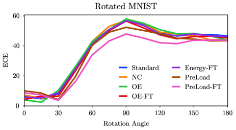
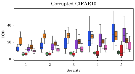
Figure 3: Calibration results, measured on the ECE metric, on Rotated MNIST and CIFAR10-C following  Ovadia et al. (2019).

5.1 Far-Away Data

We present results on two types of far-away data: FarAway (Hein et al., 2019) and FarAway Random Direction (FarAway-RD). A Faraway sample $s$ is defined as $s=tu_{x}$, where $u_{x}$ has the shape of a training sample $x$ and contains values sampled from a uniform distribution on the interval [0, 1) and $t$ is some constant. On the other hand, a FarAway-RD sample $s^{\prime}$ can be defined as $s^{\prime}=u_{x}+tv$, where $u_{x}$ and $t$ are as previously defined and $v$ is a sample from the unit sphere such that $\|v\|=1$. As the name suggests, Faraway-RD can scale the data in a random direction. For all the experiments we have fixed $t=10,000$.

Note that far-away data defined as such is unbounded, i.e. in $\mathbb{R}^{n}.$, whereas realistic images are in $[0,1]^{n}$. In the subsequent section we present results on realistic images.

Table 1 shows the FPR-$95$ metric when we evaluate on the two types of far-away data for models trained on each dataset. We observe that both versions of our method, PreLoad, and PreLoad-FT, achieve perfect FPR-$95$ of $0$ on all the datasets on both types of far-away data. The Standard method is the worst with OE also doing poorly. Energy-FT, which incorporates an energy function into the loss also does not do well in this setting. NC performs better in some scenarios such as on FarAway on MNIST but generally has high variability between different runs. DDU, which trains a Gaussian Mixture Model on top of the neural network embedding, unsurprisingly, achieves perfect results as well.

5.2 OOD Benchmarks

Next, we present our results on standard OOD benchmarks which evaluate a more realistic scenario for the evaluation of an image classifier. Models trained on MNIST and F-MNIST are evaluated on each other and E-MNIST (Cohen et al., 2017), K-MNIST (Clanuwat et al., 2018) and grey-scale CIFAR (CIFAR-Gr). Models trained on SVHN, CIFAR10 and CIFAR100 are evaluated on each other as well as LSUN classroom (LSUN-CR) (Yu et al., 2015) and Fashion MNIST 3D (FMNIST-3D). Additionally, all models are evaluated on uniform noise shaped like the relevant images and smooth noise (Hein et al., 2019), obtained by permuting, blurring and contrast-rescaling the original training data. Further information is provided in the Supplementary Section A.2.

Table 2 presents the FPR-$95$ averaged over all the OOD evaluation sets with error bars, for both the methods trained from scratch and the FT methods. Detailed results are in Section A.3. Note that we take into account the error bars when highlighting the best results. When training from scratch, PreLoad along with NC performs the best on F-MNIST, SHVN, CIFAR10, and CIFAR100. On MNIST, the NC method and OE perform better. Note that DDU which can prevent arbitrarily high confidence on far-away data is always significantly worse than our method on realistic OOD data. In the FT setting, we observe that Energy-FT is better than OE-FT, however, our FT method performs better than Energy-FT and OE-FT.

We note that extra class methods, such as NC and ours, use the confidence of the additional class to detect OOD, unlike other methods such as Standard or OE which use $\max P(y|x)$ amongst all the classes. Since the additional class is trained on OOD data, such methods tend to perform better on OOD detection.

5.3 Dataset Shifts

Once we have established that our method performs well on far-away and realistic OOD data, we evaluate model calibration under data shift. Calibration is an important measure of uncertainty quantification. We evaluate calibration using the ECE (confidence ECE following (Guo et al., 2017)) metric with $15$ bins. We use Rotated MNIST (Ovadia et al., 2019) and Corrupted CIFAR10 (CIFAR10-C) Hendrycks and Dietterich (2018) for evaluating on data shift.

We observe on Figure 3 that on Rotated MNIST, as we increase the rotation angle our two methods, trained from scratch and FT, show a lower calibration error compared to the baselines. PreLoad-FT scores the lowest ECE when the angle moves beyond $30$. On CIFAR10-C we observe that as we increase corruption severity, ECE for the Standard method degrades the most followed by NC and Energy-FT. The OE and OE-FT methods perform the best followed by our method. We observe that the FT methods do better than the methods trained from scratch.

Kristiadi et al. (2022a) suggest that NC, which is an extra class method, may do worse on dataset shift as it uses the confidence of the additional class which is trained on OOD data. Corrupted data may resemble OOD and therefore the calibration would be off. Our method on the other hand demonstrates that carefully designed extra-class methods can be better calibrated under dataset shift.

6 Conclusion

In this work, we have presented PreLoad, an OOD detection method that provably fixes arbitrarily high confidence in neural networks on far-away data. PreLoad works by training an extra class which produces larger logits as test samples move farther from the training data. Unlike all other baselines, PreLoad fulfills each of our three desiderata: a) maintain the simplicity of standard discriminative training b) provably fix arbitrarily high confidence on far-away data and c) perform well on realistic OOD samples. Future work could include training PreLoad with perturbed data such as adversarial examples, and adapting it to OOD detection in language models.

Acknowledgements

Resources used in preparing this research were provided by Huawei Canada, the Natural Sciences Engineering Council of Canada, the Province of Ontario, the Government of Canada through CIFAR, and companies sponsoring the Vector Institute.

Appendix A Supplementary Material

A.1 Training Details

We trained all models on a single 12GB-Tesla P-100 GPU. All results are averaged over 5 random seeds. Models were either trained from scratch or fine-tuned. When trained from scratch, all models were trained for 100 epochs and when fine-tuned, the Standard model was trained for 100 epochs with a further 10 epochs of fine-tuning. Note that OE-FT and Energy-FT do not introduce any new parameters to the Standard network, so all the parameters are sufficiently initialized during the 100 epochs of pre-training. On the contrary, PreLoad-FT introduces additional parameters, $w_{k+1}$ and $b_{k+1}$. In order to initialize them properly and maintain a fair comparison between the algorithms, we pre-train the new weights using the objective $\min_{w_{k+1},b_{k+1}}\mathcal{R}(f_{\psi,W}(x))$ for 10 epochs. All other parameters are frozen. After that, we fine-tune all the parameters $\theta$ using the objective $\min_{\theta}\mathcal{R}(f_{\psi,W}(x))$ where $\theta=\{\psi,W\}$ as in Algorithm 1—note that $W$ here also includes $w_{k+1}$ and $b_{k+1}$.

In all experiments, we used a batch size of 128 and a Cosine Annealing Scheduler for the learning rate. We tuned some of the hyper-parameters for PreLoad, PreLoad-FT and Energy-FT using WandB  sweeps. Each sweep consisted of 50 runs. Optimal hyper-parameter values were selected based on the highest evaluation accuracy. Table 3 lists our tuning strategy for each algorithm. Note that wd stands for weight decay, lr is learning rate, $m_{\text{in}}$ and $m_{\text{ood}}$ are the in-domian and OOD margin parameters for Energy-FT, and $\lambda$ is a constant that is multiplied to the OOD loss. Note the for Energy-FT the OOD loss has both an in-domain and an out-of-domain component

Tables 4 to 8 list the important hyper-parameters for all the methods for all the data sets. The values in bold were obtained after hyper-parameter tuning.

Table 3: Hyper-parameter Tuning Strategies

Method	Tuning Method	Parameter Ranges
Energy-FT	Random Search	$m_{\text{in}}$: -30 to 0
		$m_{\text{ood}}$: -30 to 0
PreLoad	Bayesian Optimization	lr: $1.0\times 10^{-3}$ to $5\times 10^{-1}$
		wd: $1.0\times 10^{-5}$ to $1.0\times 10^{-3}$
PreLoad-FT-Init	Random Search	$\lambda$: $1.0\times 10^{-2}$ to 1.0
		lr: $1.0\times 10^{-4}$ to $1.0\times 10^{-1}$
		wd: $1.0\times 10^{-6}$ to $1.0$
PreLoad-FT	Random Search	$\lambda$: $1.0\times 10^{-2}$ to 1.0
		lr: $1.0\times 10^{-4}$ to $1.0\times 10^{-1}$
		wd: $1.0\times 10^{-6}$ to $1.0\times 10^{-3}$

Table 4: MNIST Hyper-Parameters

Methods	Optimizer	Learning Rate	Weight Decay	$\lambda$	In Margin	Out Margin
Standard	Adam	$1.0\times 10^{-3}$	$5.0\times 10^{-4}$	-	-	-
NC	Adam	$1.0\times 10^{-3}$	$5.0\times 10^{-4}$	-	-	-
OE	Adam	$1.0\times 10^{-3}$	$5.0\times 10^{-4}$	$5.0\times 10^{-1}$	-	-
Pre-Load	Adam	$1.0\times 10^{-3}$	$5.0\times 10^{-4}$	$1.0\times 10^{0}$	-	-
OE-FT	Adam	$1.0\times 10^{-3}$	$5.0\times 10^{-4}$	$5.0\times 10^{-1}$	-	-
Energy-FT	Adam	$1.0\times 10^{-3}$	$5.0\times 10^{-4}$	$1.0\times 10^{-1}$	-3.6	-25.0
PreLoad-FT-Init	Adam	$\mathbf{4.1\times 10^{-3}}$	$\mathbf{3.1\times 10^{-4}}$	$\mathbf{8.0\times 10^{-1}}$	-	-
PreLoad-FT	Adam	$\mathbf{4.1\times 10^{-3}}$	$\mathbf{3.1\times 10^{-4}}$	$\mathbf{8.0\times 10^{-1}}$	-	-

Table 5: F-MNIST Hyper-Parameters

Methods	Optimizer	Learning Rate	Weight Decay	$\lambda$	In Margin	Out Margin
Standard	Adam	$1.0\times 10^{-3}$	$5.0\times 10^{-4}$	-	-	-
NC	Adam	$1.0\times 10^{-3}$	$5.0\times 10^{-4}$	-	-	-
OE	Adam	$1.0\times 10^{-3}$	$5.0\times 10^{-4}$	$5.0\times 10^{-1}$	-	-
Pre-Load	Adam	$1.0\times 10^{-3}$	$5.0\times 10^{-4}$	$1.0\times 10^{0}$	-	-
OE-FT	Adam	$1.0\times 10^{-3}$	$5.0\times 10^{-4}$	$5.0\times 10^{-1}$	-	-
Energy-FT	Adam	$1.0\times 10^{-3}$	$5.0\times 10^{-4}$	$1.0\times 10^{-1}$	$\mathbf{6.4\times 10^{-2}}$	-4.0
PreLoad-FT-Init	Adam	$\mathbf{6.0\times 10^{-3}}$	$\mathbf{2.5\times 10^{-3}}$	$\mathbf{2.6\times 10^{-2}}$	-	-
PreLoad-FT	Adam	$\mathbf{6.0\times 10^{-3}}$	$\mathbf{2.5\times 10^{-3}}$	$\mathbf{2.6\times 10^{-2}}$	-	-

Table 6: SVHN Hyper-Parameters

Methods	Optimizer	Learning Rate	Weight Decay	Momentum	$\lambda$	In Margin	Out Margin
Standard	SGD	$1.0\times 10^{-1}$	$5.0\times 10^{-4}$	$9.0\times 10^{-1}$	-	-	-
NC	SGD	$1.0\times 10^{-1}$	$5.0\times 10^{-4}$	$9.0\times 10^{-1}$	-	-	-
OE	SGD	$1.0\times 10^{-1}$	$5.0\times 10^{-4}$	$9.0\times 10^{-1}$	$5.0\times 10^{-1}$	-	-
Pre-Load	SGD	$1.0\times 10^{-1}$	$5.0\times 10^{-4}$	$9.0\times 10^{-1}$	$1.0\times 10^{0}$	-	-
OE-FT	SGD	$1.0\times 10^{-3}$	$5.0\times 10^{-4}$	$9.0\times 10^{-1}$	$5.0\times 10^{-}1$	-	-
Energy-FT	SGD	$1.0\times 10^{-3}$	$5.0\times 10^{-4}$	$9.0\times 10^{-1}$	$1.0\times 10^{-1}$	-5.7	-12.3
PreLoad-FT-Init	SGD	$\mathbf{2.9\times 10^{-2}}$	$\mathbf{2.8\times 10^{-6}}$	$9.0\times 10^{-1}$	$\mathbf{2.2\times 10^{-1}}$	-	-
PreLoad-FT	SGD	$\mathbf{2.9\times 10^{-2}}$	$\mathbf{2.8\times 10^{-6}}$	$9.0\times 10^{-1}$	$\mathbf{2.2\times 10^{-1}}$	-	-

Table 7: CIFAR-10 Hyper-Parameters

Methods	Optimizer	Learning Rate	Weight Decay	Momentum	$\lambda$	In Margin	Out Margin
Standard	SGD	$1.0\times 10^{-1}$	$5.0\times 10^{-4}$	$9.0\times 10^{-1}$	-	-	-
NC	SGD	$1.0\times 10^{-1}$	$5.0\times 10^{-4}$	$9.0\times 10^{-1}$	-	-	-
OE	SGD	$1.0\times 10^{-1}$	$5.0\times 10^{-4}$	$9.0\times 10^{-1}$	$5.0\times 10^{-1}$	-	-
Pre-Load	SGD	$\mathbf{7.3\times 10^{-2}}$	$\mathbf{7.6\times 10^{-4}}$	$9.0\times 10^{-1}$	$1.0\times 10^{0}$	-	-
OE-FT	SGD	$1.0\times 10^{-3}$	$5.0\times 10^{-4}$	$9.0\times 10^{-1}$	$5.0\times 10^{-1}$	-	-
Energy-FT	SGD	$1.0\times 10^{-3}$	$5.0\times 10^{-4}$	$9.0\times 10^{-1}$	$1.0\times 10^{-1}$	-9.9	-5.7
PreLoad-FT-Init	SGD	$\mathbf{6.1\times 10^{-2}}$	$\mathbf{1.8\times 10^{-6}}$	$9.0\times 10^{-1}$	$\mathbf{2.0\times 10^{-2}}$	-	-
PreLoad-FT	SGD	$\mathbf{6.1\times 10^{-2}}$	$\mathbf{1.8\times 10^{-6}}$	$9.0\times 10^{-1}$	$\mathbf{2.0\times 10^{-2}}$	-	-

Table 8: CIFAR-100 Hyper-Parameters

Methods	Optimizer	Learning Rate	Weight Decay	Momentum	$\lambda$	In Margin	Out Margin
Standard	SGD	$1.0\times 10^{-1}$	$5.0\times 10^{-4}$	$9.0\times 10^{-1}$	-	-	-
NC	SGD	$1.0\times 10^{-1}$	$5.0\times 10^{-4}$	$9.0\times 10^{-1}$	-	-	-
OE	SGD	$1.0\times 10^{-1}$	$5.0\times 10^{-4}$	$9.0\times 10^{-1}$	$5.0\times 10^{-1}$	-	-
Pre-Load	SGD	$\mathbf{4.5\times 10^{-1}}$	$\mathbf{1.2\times 10^{-4}}$	$9.0\times 10^{-1}$	$1.0\times 10^{0}$	-	-
OE-FT	SGD	$1.0\times 10^{-3}$	$5.0\times 10^{-4}$	$9.0\times 10^{-1}$	$5.0\times 10^{-1}$	-	-
Energy-FT	SGD	$1.0\times 10^{-3}$	$5.0\times 10^{-4}$	$9.0\times 10^{-1}$	$1.0\times 10^{-1}$	-14.5	-10.3
PreLoad-FT-Init	SGD	$\mathbf{6.3\times 10^{-3}}$	$\mathbf{1.1\times 10^{-4}}$	$9.0\times 10^{-1}$	$\mathbf{2.3\times 10^{-2}}$	-	-
PreLoad-FT	SGD	$\mathbf{6.3\times 10^{-3}}$	$\mathbf{1.1\times 10^{-4}}$	$9.0\times 10^{-1}$	$\mathbf{2.3\times 10^{-2}}$	-	-

A.2 OOD Test Sets

In addition to MNIST, F-MNIST, SVHN, CIFAR-10 and CIFAR-100, we evaluate on the following OOD test sets.

• E-MNIST consists of handwritten letters and is in the same format as MNIST (Cohen et al., 2017).

• K-MNIST consists of handwritten Japanese (Hiragana script) and is in the same format as MNIST (Clanuwat et al., 2018).

• CIFAR-Gr consists of CIFAR-10 images converted to greyscale.

• LSUN-CR consists of real images of classrooms (Yu et al., 2015).

• FMNIST-$3$D consists of F-MNIST images converted from single channel to three channels with identical values.

A.3 Additional Results

In Table 9, we present the complete FPR-$95$ results for all the methods and datasets that were used to compute the average results reported in Table 2. Note that results for Far-Away and Far-Away-RD are not included in the averages. Additionally, Table 10 presents results with the AUROC metric. AUROC is the area under the receiver operator curve (ROC). The ROC plots the TPR against FPR. AUROC can be interpreted as the probability that a model under test ranks a random positive sample higher than a random negative sample. We report AUROC as a percentage between 0 and 100 where higher the better.

Tables 11 and 12 present the accuracy and calibration scores respectively.

Table 9: FPR-95, Complete Results

Datasets	Standard	DDU	NC	OE	PreLoad	OE-FT	Energy-FT	PreLoad-FT
MNIST
F-MNIST	8.1$\pm$0.9	21.8$\pm$1.1	0.0$\pm$0.0	0.2$\pm$0.0	0.0$\pm$0.0	0.3$\pm$0.1	3.7$\pm$0.7	0.1$\pm$0.0
E-MNIST	32.1$\pm$0.4	18.5$\pm$0.3	17.0$\pm$0.5	27.4$\pm$0.2	29.7$\pm$0.4	24.8$\pm$0.3	36.5$\pm$0.3	33.1$\pm$2.8
K-MNIST	10.9$\pm$0.3	4.6$\pm$0.1	3.1$\pm$0.4	5.4$\pm$0.2	9.8$\pm$0.6	3.4$\pm$0.2	10.1$\pm$0.6	17.2$\pm$3.5
CIFAR-Gr	0.0$\pm$0.0	62.6$\pm$8.2	0.0$\pm$0.0	0.0$\pm$0.0	0.0$\pm$0.0	0.0$\pm$0.0	0.0$\pm$0.0	0.0$\pm$0.0
Uniform	14.1$\pm$7.8	81.3$\pm$13.1	0.0$\pm$0.0	0.0$\pm$0.0	0.0$\pm$0.0	0.0$\pm$0.0	0.0$\pm$0.0	0.0$\pm$0.0
Smooth	0.0$\pm$0.0	97.5$\pm$2.4	0.0$\pm$0.0	0.0$\pm$0.0	0.0$\pm$0.0	0.0$\pm$0.0	0.0$\pm$0.0	0.0$\pm$0.0
FarAway	100.0$\pm$0.0	0.0$\pm$0.0	0.0$\pm$0.0	56.6$\pm$19.6	0.0$\pm$0.0	99.0$\pm$0.4	100.0$\pm$0.0	0.0$\pm$0.0
FarAway-RD	99.9$\pm$0.0	0.0$\pm$0.0	99.9$\pm$0.1	99.8$\pm$0.0	0.0$\pm$0.0	99.5$\pm$0.1	100.0$\pm$0.0	0.0$\pm$0.0
F-MNIST
MNIST	74.8$\pm$1.4	0.6$\pm$0.2	6.8$\pm$0.5	65.4$\pm$1.1	6.7$\pm$2.1	68.4$\pm$1.5	36.9$\pm$3.5	28.8$\pm$3.4
E-MNIST	72.3$\pm$0.7	2.6$\pm$0.6	1.7$\pm$0.2	55.4$\pm$1.6	1.4$\pm$0.3	60.4$\pm$0.8	28.5$\pm$1.7	15.2$\pm$3.2
K-MNIST	73.6$\pm$0.6	0.4$\pm$0.1	4.7$\pm$0.6	58.1$\pm$0.9	5.7$\pm$1.2	60.6$\pm$1.0	21.1$\pm$1.3	22.6$\pm$2.6
CIFAR-Gr	85.4$\pm$1.0	84.3$\pm$3.8	0.0$\pm$0.0	0.0$\pm$0.0	0.0$\pm$0.0	0.1$\pm$0.0	0.1$\pm$0.0	0.0$\pm$0.0
Uniform	91.9$\pm$2.8	33.2$\pm$18.9	0.1$\pm$0.1	11.3$\pm$9.6	0.0$\pm$0.0	0.3$\pm$0.2	0.3$\pm$0.1	2.0$\pm$1.3
Smooth	25.6$\pm$1.4	89.6$\pm$0.6	0.0$\pm$0.0	0.2$\pm$0.0	0.0$\pm$0.0	0.4$\pm$0.1	0.2$\pm$0.1	5.8$\pm$5.8
FarAway	100.0$\pm$0.0	0.0$\pm$0.0	53.5$\pm$22.5	100.0$\pm$0.0	0.0$\pm$0.0	100.0$\pm$0.0	38.4$\pm$8.9	0.0$\pm$0.0
FarAway-RD	100.0$\pm$0.0	0.0$\pm$0.0	100.0$\pm$0.0	100.0$\pm$0.0	0.0$\pm$0.0	100.0$\pm$0.0	81.6$\pm$8.8	0.0$\pm$0.0
SVHN
CIFAR-10	20.2$\pm$0.6	8.3$\pm$0.5	0.0$\pm$0.0	0.0$\pm$0.0	0.0$\pm$0.0	0.1$\pm$0.0	4.7$\pm$0.2	0.0$\pm$0.0
LSUN-CR	24.8$\pm$0.9	2.5$\pm$0.5	0.0$\pm$0.0	0.0$\pm$0.0	0.0$\pm$0.0	0.0$\pm$0.0	3.5$\pm$0.3	0.0$\pm$0.0
CIFAR-100	23.4$\pm$0.6	8.9$\pm$0.4	0.0$\pm$0.0	0.1$\pm$0.0	0.0$\pm$0.0	0.5$\pm$0.0	7.5$\pm$0.2	0.0$\pm$0.0
FMNIST-3D	26.5$\pm$0.4	25.8$\pm$2.2	0.0$\pm$0.0	0.0$\pm$0.0	0.0$\pm$0.0	0.6$\pm$0.3	14.9$\pm$1.1	0.0$\pm$0.0
Uniform	33.5$\pm$3.9	0.0$\pm$0.0	0.0$\pm$0.0	0.0$\pm$0.0	0.0$\pm$0.0	0.0$\pm$0.0	0.9$\pm$0.1	0.0$\pm$0.0
Smooth	14.0$\pm$0.5	2.5$\pm$0.4	12.6$\pm$1.2	10.0$\pm$0.3	6.8$\pm$1.0	8.6$\pm$0.3	11.8$\pm$1.3	4.6$\pm$0.2
FarAway	99.4$\pm$0.2	0.0$\pm$0.0	80.0$\pm$20.0	99.4$\pm$0.4	0.0$\pm$0.0	99.3$\pm$0.3	100.0$\pm$0.0	0.0$\pm$0.0
FarAway-RD	92.8$\pm$2.1	0.0$\pm$0.0	80.0$\pm$20.0	85.4$\pm$7.6	0.0$\pm$0.0	93.1$\pm$2.5	100.0$\pm$0.0	0.0$\pm$0.0
CIFAR-10
SVHN	42.1$\pm$6.5	45.1$\pm$2.4	0.5$\pm$0.1	2.7$\pm$0.6	0.4$\pm$0.1	8.1$\pm$2.2	2.9$\pm$0.6	4.4$\pm$2.1
LSUN-CR	50.1$\pm$1.1	64.1$\pm$1.7	0.6$\pm$0.1	6.1$\pm$0.3	0.7$\pm$0.2	20.7$\pm$1.2	7.9$\pm$0.3	4.3$\pm$0.2
CIFAR-100	58.8$\pm$0.6	71.0$\pm$0.4	26.5$\pm$0.1	33.4$\pm$0.3	27.3$\pm$0.1	44.9$\pm$0.4	34.0$\pm$0.3	35.9$\pm$0.2
FMNIST-3D	38.9$\pm$1.1	35.7$\pm$5.4	3.5$\pm$0.4	11.5$\pm$0.6	3.9$\pm$0.4	15.8$\pm$1.0	8.2$\pm$0.6	7.9$\pm$0.8
Uniform	76.3$\pm$15.5	0.0$\pm$0.0	0.0$\pm$0.0	0.0$\pm$0.0	0.0$\pm$0.0	0.0$\pm$0.0	19.8$\pm$19.6	0.0$\pm$0.0
Smooth	40.4$\pm$5.1	12.4$\pm$1.8	3.4$\pm$0.7	16.3$\pm$3.0	3.6$\pm$0.6	30.2$\pm$1.5	20.6$\pm$2.6	19.4$\pm$6.0
FarAway	100.0$\pm$0.0	0.0$\pm$0.0	20.0$\pm$20.0	100.0$\pm$0.0	0.0$\pm$0.0	100.0$\pm$0.0	100.0$\pm$0.0	0.0$\pm$0.0
FarAway-RD	99.7$\pm$0.2	0.0$\pm$0.0	40.0$\pm$24.5	100.0$\pm$0.0	0.0$\pm$0.0	99.5$\pm$0.3	100.0$\pm$0.0	0.0$\pm$0.0
CIFAR-100
SVHN	71.0$\pm$1.1	82.4$\pm$4.1	21.9$\pm$5.3	60.2$\pm$3.0	19.0$\pm$2.6	68.2$\pm$1.8	50.0$\pm$6.1	46.1$\pm$6.5
LSUN-CR	78.1$\pm$0.7	88.1$\pm$0.6	12.1$\pm$0.8	62.8$\pm$2.1	17.7$\pm$0.6	71.7$\pm$0.8	48.9$\pm$1.1	36.6$\pm$0.7
CIFAR-10	79.2$\pm$0.4	92.8$\pm$0.1	79.4$\pm$0.3	80.7$\pm$0.4	80.5$\pm$0.6	80.1$\pm$0.6	79.7$\pm$0.3	88.9$\pm$0.1
FMNIST-3D	65.6$\pm$2.2	90.2$\pm$0.9	7.2$\pm$0.5	56.0$\pm$3.0	13.9$\pm$1.5	61.3$\pm$1.6	34.4$\pm$3.6	46.4$\pm$2.8
Uniform	96.6$\pm$3.3	0.0$\pm$0.0	0.0$\pm$0.0	41.0$\pm$22.1	0.0$\pm$0.0	75.8$\pm$14.6	22.7$\pm$19.1	0.0$\pm$0.0
Smooth	72.7$\pm$1.3	42.5$\pm$1.2	44.1$\pm$4.9	60.4$\pm$3.4	24.2$\pm$4.1	66.6$\pm$1.2	61.0$\pm$2.7	19.0$\pm$3.7
FarAway	100.0$\pm$0.0	0.0$\pm$0.0	20.0$\pm$20.0	100.0$\pm$0.0	0.0$\pm$0.0	100.0$\pm$0.0	100.0$\pm$0.0	0.0$\pm$0.0
FarAway-RD	100.0$\pm$0.0	0.0$\pm$0.0	20.0$\pm$20.0	100.0$\pm$0.0	0.0$\pm$0.0	100.0$\pm$0.0	100.0$\pm$0.0	0.0$\pm$0.0

Table 10: AUROC, Complete Results

Datasets	Standard	DDU	NC	OE	PreLoad	OE-FT	Energy-FT	PreLoad-FT
MNIST
F-MNIST	98.3$\pm$0.1	96.9$\pm$0.1	100.0$\pm$0.0	99.8$\pm$0.0	100.0$\pm$0.0	99.7$\pm$0.0	99.2$\pm$0.2	100.0$\pm$0.0
E-MNIST	90.2$\pm$0.1	91.6$\pm$0.1	96.4$\pm$0.1	92.8$\pm$0.0	89.0$\pm$0.2	93.7$\pm$0.1	90.2$\pm$0.1	87.7$\pm$1.1
K-MNIST	97.5$\pm$0.1	98.9$\pm$0.0	99.3$\pm$0.1	98.6$\pm$0.1	97.5$\pm$0.2	99.0$\pm$0.1	97.7$\pm$0.1	95.2$\pm$1.1
CIFAR-Gr	99.8$\pm$0.0	94.3$\pm$0.4	100.0$\pm$0.0	100.0$\pm$0.0	100.0$\pm$0.0	100.0$\pm$0.0	100.0$\pm$0.0	100.0$\pm$0.0
Uniform	96.7$\pm$0.5	93.2$\pm$0.8	100.0$\pm$0.0	100.0$\pm$0.0	100.0$\pm$0.0	100.0$\pm$0.0	99.6$\pm$0.1	100.0$\pm$0.0
Smooth	100.0$\pm$0.0	89.4$\pm$2.7	100.0$\pm$0.0	100.0$\pm$0.0	100.0$\pm$0.0	100.0$\pm$0.0	100.0$\pm$0.0	100.0$\pm$0.0
FarAway	1.1$\pm$0.1	100.0$\pm$0.0	100.0$\pm$0.0	59.8$\pm$16.0	100.0$\pm$0.0	7.3$\pm$4.6	0.0$\pm$0.0	100.0$\pm$0.0
FarAway-RD	1.2$\pm$0.1	100.0$\pm$0.0	16.4$\pm$1.0	1.5$\pm$0.1	100.0$\pm$0.0	2.1$\pm$0.3	0.0$\pm$0.0	100.0$\pm$0.0
F-MNIST
MNIST	80.1$\pm$0.6	99.7$\pm$0.1	98.4$\pm$0.1	84.4$\pm$0.7	98.4$\pm$0.5	82.9$\pm$0.4	90.5$\pm$1.0	92.4$\pm$1.2
E-MNIST	82.6$\pm$0.4	99.3$\pm$0.1	99.6$\pm$0.1	88.8$\pm$0.7	99.7$\pm$0.1	87.5$\pm$0.6	93.5$\pm$0.4	96.1$\pm$1.0
K-MNIST	83.1$\pm$0.4	99.7$\pm$0.0	99.0$\pm$0.1	89.9$\pm$0.2	98.9$\pm$0.2	89.1$\pm$0.1	95.7$\pm$0.3	95.1$\pm$0.6
CIFAR-Gr	83.8$\pm$0.6	85.0$\pm$1.2	100.0$\pm$0.0	100.0$\pm$0.0	100.0$\pm$0.0	100.0$\pm$0.0	99.8$\pm$0.0	100.0$\pm$0.0
Uniform	74.3$\pm$3.3	95.7$\pm$1.2	99.9$\pm$0.1	98.6$\pm$1.1	100.0$\pm$0.0	99.9$\pm$0.0	99.8$\pm$0.1	99.6$\pm$0.3
Smooth	95.9$\pm$0.2	59.5$\pm$1.2	100.0$\pm$0.0	100.0$\pm$0.0	100.0$\pm$0.0	99.9$\pm$0.0	99.1$\pm$0.0	98.6$\pm$1.3
FarAway	2.6$\pm$0.2	100.0$\pm$0.0	49.0$\pm$21.5	2.2$\pm$0.3	100.0$\pm$0.0	1.8$\pm$0.2	61.6$\pm$8.9	100.0$\pm$0.0
FarAway-RD	2.8$\pm$0.2	100.0$\pm$0.0	5.3$\pm$0.5	2.3$\pm$0.2	100.0$\pm$0.0	1.7$\pm$0.2	18.5$\pm$8.8	100.0$\pm$0.0
SVHN
CIFAR-10	95.9$\pm$0.1	98.3$\pm$0.1	100.0$\pm$0.0	100.0$\pm$0.0	100.0$\pm$0.0	99.9$\pm$0.0	98.8$\pm$0.0	100.0$\pm$0.0
LSUN-CR	95.6$\pm$0.1	99.1$\pm$0.0	100.0$\pm$0.0	100.0$\pm$0.0	100.0$\pm$0.0	100.0$\pm$0.0	99.1$\pm$0.1	100.0$\pm$0.0
CIFAR-100	95.1$\pm$0.1	98.2$\pm$0.1	100.0$\pm$0.0	100.0$\pm$0.0	100.0$\pm$0.0	99.9$\pm$0.0	98.2$\pm$0.0	100.0$\pm$0.0
FMNIST-3D	94.5$\pm$0.4	96.0$\pm$0.3	100.0$\pm$0.0	100.0$\pm$0.0	100.0$\pm$0.0	99.7$\pm$0.1	96.9$\pm$0.3	100.0$\pm$0.0
Uniform	93.2$\pm$0.9	100.0$\pm$0.0	100.0$\pm$0.0	100.0$\pm$0.0	100.0$\pm$0.0	100.0$\pm$0.0	99.6$\pm$0.0	100.0$\pm$0.0
Smooth	96.9$\pm$0.2	99.2$\pm$0.1	97.1$\pm$0.3	98.0$\pm$0.1	98.4$\pm$0.2	98.3$\pm$0.1	97.4$\pm$0.2	98.9$\pm$0.0
FarAway	1.8$\pm$0.6	100.0$\pm$0.0	20.2$\pm$20.0	2.0$\pm$1.2	100.0$\pm$0.0	3.9$\pm$1.1	0.0$\pm$0.0	100.0$\pm$0.0
FarAway-RD	19.9$\pm$5.9	100.0$\pm$0.0	20.2$\pm$20.0	38.0$\pm$16.5	100.0$\pm$0.0	23.0$\pm$7.2	0.0$\pm$0.0	100.0$\pm$0.0
CIFAR-10
SVHN	94.4$\pm$1.0	91.1$\pm$0.5	99.6$\pm$0.1	99.4$\pm$0.1	99.7$\pm$0.1	98.6$\pm$0.3	98.9$\pm$0.1	99.1$\pm$0.3
LSUN-CR	92.6$\pm$0.2	87.4$\pm$0.3	99.7$\pm$0.0	99.0$\pm$0.0	99.7$\pm$0.0	97.1$\pm$0.1	98.4$\pm$0.0	99.1$\pm$0.0
CIFAR-100	90.0$\pm$0.0	80.7$\pm$0.2	94.9$\pm$0.0	94.1$\pm$0.1	94.3$\pm$0.1	92.3$\pm$0.1	93.4$\pm$0.0	92.9$\pm$0.0
FMNIST-3D	94.7$\pm$0.2	94.5$\pm$0.8	99.3$\pm$0.1	98.3$\pm$0.1	99.1$\pm$0.1	97.7$\pm$0.1	98.4$\pm$0.1	98.5$\pm$0.2
Uniform	88.2$\pm$3.0	100.0$\pm$0.0	99.8$\pm$0.2	100.0$\pm$0.0	99.8$\pm$0.0	100.0$\pm$0.0	97.4$\pm$1.8	100.0$\pm$0.0
Smooth	93.6$\pm$1.1	96.1$\pm$0.7	99.0$\pm$0.1	97.5$\pm$0.4	98.9$\pm$0.1	96.3$\pm$0.4	96.9$\pm$0.4	97.1$\pm$0.7
FarAway	3.4$\pm$0.1	100.0$\pm$0.0	80.1$\pm$19.9	3.6$\pm$0.0	100.0$\pm$0.0	5.1$\pm$0.3	0.0$\pm$0.0	100.0$\pm$0.0
FarAway-RD	5.0$\pm$1.3	100.0$\pm$0.0	60.3$\pm$24.3	3.6$\pm$0.0	100.0$\pm$0.0	10.1$\pm$3.6	0.0$\pm$0.0	100.0$\pm$0.0
CIFAR-100
SVHN	82.9$\pm$0.5	72.0$\pm$2.4	96.1$\pm$0.9	86.7$\pm$0.7	96.6$\pm$0.3	84.0$\pm$0.9	91.7$\pm$1.0	92.1$\pm$1.0
LSUN-CR	80.1$\pm$0.5	73.5$\pm$0.6	97.4$\pm$0.1	86.6$\pm$0.4	96.6$\pm$0.0	83.0$\pm$0.4	92.0$\pm$0.2	93.6$\pm$0.1
CIFAR-10	77.4$\pm$0.2	65.7$\pm$0.3	80.8$\pm$0.1	77.2$\pm$0.2	79.1$\pm$0.5	77.1$\pm$0.2	79.3$\pm$0.1	73.9$\pm$0.2
FMNIST-3D	85.2$\pm$0.9	67.6$\pm$1.1	98.3$\pm$0.1	88.4$\pm$0.7	97.2$\pm$0.2	86.5$\pm$0.6	94.7$\pm$0.5	92.8$\pm$0.4
Uniform	62.3$\pm$7.7	99.9$\pm$0.1	100.0$\pm$0.0	87.1$\pm$8.5	100.0$\pm$0.0	73.8$\pm$10.2	95.9$\pm$2.9	100.0$\pm$0.0
Smooth	75.4$\pm$1.2	84.9$\pm$2.2	89.9$\pm$1.2	81.1$\pm$1.3	95.1$\pm$1.0	78.3$\pm$0.7	82.7$\pm$1.5	96.1$\pm$0.8
FarAway	0.4$\pm$0.0	100.0$\pm$0.0	80.2$\pm$19.8	0.8$\pm$0.0	100.0$\pm$0.0	0.9$\pm$0.1	0.0$\pm$0.0	100.0$\pm$0.0
FarAway-RD	1.1$\pm$0.3	100.0$\pm$0.0	80.2$\pm$19.8	0.9$\pm$0.2	100.0$\pm$0.0	1.0$\pm$0.1	0.0$\pm$0.0	100.0$\pm$0.0

Table 11: Accuracy

	MNIST	F-MNIST	SVHN	CIFAR-10	CIFAR-100
Standard	99.5	92.7	97.4	94.9	77.3
DDU	99.5	92.7	97.4	94.9	77.3
NC	99.4	92.6	97.3	92.8	73.6
OE	99.5	92.7	97.4	95.5	77.1
PreLoad	99.5	92.3	97.3	93.5	71.9
OE-FT	99.5	92.8	97.3	94.8	77.1
Energy-FT	99.5	92.8	97.4	94.9	76.8
PreLoad-FT	99.5	92.4	97.1	94.5	76.8

Table 12: Calibration measured using the ECE score

	MNIST	F-MNIST	SVHN	CIFAR-10	CIFAR-100
Standard	7.1	12.2	8.9	10.6	13.3
DDU	7.1	12.2	8.9	10.6	13.3
NC	7.1	7.4	9.0	15.2	8.6
OE	6.4	11.5	9.1	6.1	13.1
PreLoad	8.9	6.1	7.3	11.9	9.8
OE-FT	7.1	11.6	10.0	5.7	16.0
Energy-FT	6.7	11.8	12.2	10.3	15.5
PreLoad-FT	8.6	3.9	10.3	8.1	11.1

References

- Guo et al. (2017) Chuan Guo, Geoff Pleiss, Yu Sun, and Kilian Q Weinberger. On calibration of modern Neural Networks. In International Conference on Machine Learning. PMLR, 2017.
- Nguyen et al. (2015) Anh Nguyen, Jason Yosinski, and Jeff Clune. Deep Neural Networks are easily fooled: High confidence predictions for unrecognizable images. In Proceedings of the IEEE conference on computer vision and pattern recognition, 2015.
- Hein et al. (2019) Matthias Hein, Maksym Andriushchenko, and Julian Bitterwolf. Why ReLU networks yield high-confidence predictions far away from the training data and how to mitigate the problem. In Proceedings of the IEEE/CVF Conference on Computer Vision and Pattern Recognition, 2019.
- Gupta et al. (2020) Kartik Gupta, Amir Rahimi, Thalaiyasingam Ajanthan, Thomas Mensink, Cristian Sminchisescu, and Richard Hartley. Calibration of Neural Networks using Splines. In International Conference on Learning Representations, 2020.
- Kull et al. (2019) Meelis Kull, Miquel Perello Nieto, Markus Kängsepp, Telmo Silva Filho, Hao Song, and Peter Flach. Beyond temperature scaling: Obtaining well-calibrated multi-class probabilities with Dirichlet calibration. Advances in neural information processing systems, 32, 2019.
- Müller et al. (2019) Rafael Müller, Simon Kornblith, and Geoffrey E Hinton. When does Label Smoothing help? Advances in neural information processing systems, 32, 2019.
- Thulasidasan et al. (2019) Sunil Thulasidasan, Gopinath Chennupati, Jeff A Bilmes, Tanmoy Bhattacharya, and Sarah Michalak. On Mixup training: Improved calibration and predictive uncertainty for deep Neural Networks. Advances in Neural Information Processing Systems, 32, 2019.
- Kumar et al. (2018) Aviral Kumar, Sunita Sarawagi, and Ujjwal Jain. Trainable calibration measures for Neural Networks from kernel mean embeddings. In International Conference on Machine Learning. PMLR, 2018.
- Lin et al. (2017) Tsung-Yi Lin, Priya Goyal, Ross Girshick, Kaiming He, and Piotr Dollár. Focal loss for dense object detection. In Proceedings of the IEEE international conference on computer vision, 2017.
- Minderer et al. (2021) Matthias Minderer, Josip Djolonga, Rob Romijnders, Frances Hubis, Xiaohua Zhai, Neil Houlsby, Dustin Tran, and Mario Lucic. Revisiting the calibration of modern Neural Networks. In M. Ranzato, A. Beygelzimer, Y. Dauphin, P.S. Liang, and J. Wortman Vaughan, editors, Advances in Neural Information Processing Systems, volume 34. Curran Associates, Inc., 2021.
- Blundell et al. (2015) Charles Blundell, Julien Cornebise, Koray Kavukcuoglu, and Daan Wierstra. Weight uncertainty in Neural Network. In International Conference on Machine Learning. PMLR, 2015.
- Gal and Ghahramani (2016) Yarin Gal and Zoubin Ghahramani. Dropout as a Bayesian approximation: Representing model uncertainty in deep learning. In International Conference on Machine Learning. PMLR, 2016.
- Kristiadi et al. (2020) Agustinus Kristiadi, Matthias Hein, and Philipp Hennig. Being Bayesian, even just a bit, fixes overconfidence in ReLU Networks. In International Conference on Machine Learning. PMLR, 2020.
- Lakshminarayanan et al. (2017) Balaji Lakshminarayanan, Alexander Pritzel, and Charles Blundell. Simple and scalable predictive uncertainty estimation using Deep Ensembles. Advances in neural information processing systems, 30, 2017.
- Mukhoti et al. (2023) Jishnu Mukhoti, Andreas Kirsch, Joost van Amersfoort, Philip HS Torr, and Yarin Gal. Deep deterministic uncertainty: A new simple baseline. In Proceedings of the IEEE/CVF Conference on Computer Vision and Pattern Recognition, 2023.
- Zhang and LeCun (2017) Xiang Zhang and Yann LeCun. Universum prescription: Regularization using unlabeled data. In Proceedings of the AAAI Conference on Artificial Intelligence, volume 31, 2017.
- Kristiadi et al. (2022a) Agustinus Kristiadi, Matthias Hein, and Philipp Hennig. Being a bit frequentist improves bayesian Neural Networks. In International Conference on Artificial Intelligence and Statistics. PMLR, 2022a.
- Hendrycks et al. (2018) Dan Hendrycks, Mantas Mazeika, and Thomas Dietterich. Deep anomaly detection with Outlier Exposure. In International Conference on Learning Representations, 2018.
- Lee et al. (2018) Kimin Lee, Kibok Lee, Honglak Lee, and Jinwoo Shin. A simple unified framework for detecting out-of-distribution samples and Adversarial Attacks. Advances in Neural Information Processing Systems, 31, 2018.
- Meinke and Hein (2020) Alexander Meinke and Matthias Hein. Towards Neural Networks that provably know when they don’t know. In International Conference on Learning Representations, 2020.
- (21) Christos Louizos and Max Welling. Multiplicative normalizing flows for variational Bayesian Neural Networks. In International Conference on Machine Learning.
- Kristiadi et al. (2022b) Agustinus Kristiadi, Runa Eschenhagen, and Philipp Hennig. Posterior refinement improves sample efficiency in Bayesian Neural Networks. 2022b.
- Kristiadi et al. (2021) Agustinus Kristiadi, Matthias Hein, and Philipp Hennig. An infinite-feature extension for Bayesian ReLU nets that fixes their asymptotic overconfidence. Advances in Neural Information Processing Systems, 34, 2021.
- Arora et al. (2018) Raman Arora, Amitabh Basu, Poorya Mianjy, and Anirbit Mukherjee. Understanding deep Neural Networks with rectified linear units. In International Conference on Learning Representations, 2018.
- Goodfellow et al. (2014) Ian Goodfellow, Jean Pouget-Abadie, Mehdi Mirza, Bing Xu, David Warde-Farley, Sherjil Ozair, Aaron Courville, and Yoshua Bengio. Generative adversarial nets. Advances in Neural Information Processing Systems, 27, 2014.
- Kingma and Welling (2013) Diederik P Kingma and Max Welling. Auto-encoding variational Bayes. arXiv preprint arXiv:1312.6114, 2013.
- Liu et al. (2020) Weitang Liu, Xiaoyun Wang, John Owens, and Yixuan Li. Energy-based out-of-distribution detection. Advances in Neural Information Processing Systems, 33, 2020.
- LeCun et al. (1998) Yann LeCun, Léon Bottou, Yoshua Bengio, and Patrick Haffner. Gradient-based learning applied to document recognition. Proceedings of the IEEE, 86(11), 1998.
- Xiao et al. (2017) Han Xiao, Kashif Rasul, and Roland Vollgraf. Fashion-mnist: a novel image dataset for benchmarking machine learning algorithms. arXiv preprint arXiv:1708.07747, 2017.
- Netzer et al. (2011) Yuval Netzer, Tao Wang, Adam Coates, Alessandro Bissacco, Bo Wu, and Andrew Y Ng. Reading digits in natural images with unsupervised feature learning. 2011.
- Krizhevsky et al. (2009) Alex Krizhevsky et al. Learning multiple layers of features from tiny images. 2009.
- Zagoruyko and Komodakis (2016) Sergey Zagoruyko and Nikos Komodakis. Wide Residual Networks. arXiv preprint arXiv:1605.07146, 2016.
- Torralba et al. (2008) Antonio Torralba, Rob Fergus, and William T Freeman. 80 million tiny images: A large data set for nonparametric object and scene recognition. IEEE transactions on Pattern Analysis and Machine Intelligence, 30(11), 2008.
- Henriksson et al. (2021) Jens Henriksson, Christian Berger, Markus Borg, Lars Tornberg, Sankar Raman Sathyamoorthy, and Cristofer Englund. Performance analysis of out-of-distribution detection on trained Neural Networks. Information and Software Technology, 130, 2021.
- Ovadia et al. (2019) Yaniv Ovadia, Emily Fertig, Jie Ren, Zachary Nado, David Sculley, Sebastian Nowozin, Joshua Dillon, Balaji Lakshminarayanan, and Jasper Snoek. Can you trust your model’s uncertainty? evaluating predictive uncertainty under dataset shift. Advances in Neural Information Processing Systems, 32, 2019.
- Cohen et al. (2017) Gregory Cohen, Saeed Afshar, Jonathan Tapson, and Andre Van Schaik. Emnist: Extending MNIST to handwritten letters. In 2017 international joint conference on Neural Networks. IEEE, 2017.
- Clanuwat et al. (2018) Tarin Clanuwat, Mikel Bober-Irizar, Asanobu Kitamoto, Alex Lamb, Kazuaki Yamamoto, and David Ha. Deep learning for classical japanese literature. arXiv preprint arXiv:1812.01718, 2018.
- Yu et al. (2015) Fisher Yu, Ari Seff, Yinda Zhang, Shuran Song, Thomas Funkhouser, and Jianxiong Xiao. Lsun: Construction of a large-scale image dataset using deep learning with humans in the loop. arXiv preprint arXiv:1506.03365, 2015.
- Hendrycks and Dietterich (2018) Dan Hendrycks and Thomas Dietterich. Benchmarking Neural Network robustness to common corruptions and perturbations. In International Conference on Learning Representations, 2018.