Deep Bayesian Reinforcement Learning for
Spacecraft Proximity Maneuvers and Docking

Abstract

In the pursuit of autonomous spacecraft proximity maneuvers and docking(PMD), we introduce a novel Bayesian actor-critic reinforcement learning algorithm to learn a control policy with the stability guarantee. The PMD task is formulated as a Markov decision process that reflects the relative dynamic model, the docking cone and the cost function. Drawing from the principles of Lyapunov theory, we frame the temporal difference learning as a constrained Gaussian process regression problem. This innovative approach allows the state-value function to be expressed as a Lyapunov function, leveraging the Gaussian process and deep kernel learning. We develop a novel Bayesian quadrature policy optimization procedure to analytically compute the policy gradient while integrating Lyapunov-based stability constraints. This integration is pivotal in satisfying the rigorous safety demands of spaceflight missions. The proposed algorithm has been experimentally evaluated on a spacecraft air-bearing testbed and shows impressive and promising performance.

1 Introduction

Bayesian reinforcement learning (BRL) is an elegant approach to reinforcement learning (RL) [1] that leverages methods from Bayesian inference to incorporate information into the learning process [2]. In BRL, the prior information can be expressed as a probabilistic distribution, and new information can be incorporated using standard rules of Bayesian inference [2, 3, 4]. For example, the information can be encoded and updated in the value function [3]. In this paper, we integrate the Bayesian actor-critic (BAC) RL algorithm with deep learning and deep kernel learning techniques [5] for high-dimensional continuous robot control tasks. The critic is modeled explicitly through Gaussian process temporal difference (GPTD) and deep kernel learning [3, 5], while the actor is modeled as a standard deep neural network. The policy gradient integral can be efficiently approximated with a significantly low estimate variance using Gaussian process [6] , compared with Monte-Carlo (MC) sampling, using Bayesian Quadrature (BQ) [7] from probabilistic numerics [8] or the recently proposed deep BQ method [9] to high dimensional settings.

Robot control tasks often involve stability requirements where the controller must be guaranteed to drive the system towards a goal state, and it could recover to the goal state even in the presence of parametric uncertainties and disturbances [10]. Lyapunov’s theory [11] provides a principled method for studying the stability of robotic systems, by constructing a scalar “energy” function, known as a Lyapunov function, that decreases over time. Recently, there is a rich list of literature on learning/data-driven control with stability (and safety) guarantee by learning a Lyapunov function using data (either from complete trajectories or random samples), regardless RL is used or not [12, 13, 14, 15, 16]. Thereafter, the policy/controller can be sought after using the conceptual optimisation procedure as follows (or its relaxations [12, 15]):

optimize $$\ \ \ \ \ \text{policy/controller},$$ (1)

subject to $$V$$ is a Lyapunov function (2)

The key problem is that an accurate system model should be given a priori under certain assumptions of the model type and parameter distributions. Moreover, crucially, the dimension of the system is typically low, which prevents the applicability for high-dimensional continuous control tasks, such as MuJoCo [17]. To address this issue, in our previous work [18], a data-based (model-free) approach is proposed by substituting $V$ in $\eqref{opti-problem-2}$ with $\mathbb{E}_{\text{data}}V$ in the policy optimization procedure $\eqref{opti-problem-1}$ based on the soft actor-critic algorithm [19] and has to choose the state-action function to be the Lyapunov function.

This paper proposes a novel framework for BAC RL algorithm with a stability guarantee based on Lyapunov theory. The contribution of this paper has three parts:

• We provide a novel formulation of the Lyapunov function in Bayesian RL as a constrained Gaussian process regression problem and solve it analytically using a truncated Gaussian process.

• We develop a novel Bayesian quadrature policy optimization procedure to analytically compute the policy gradient integral with Lyapunov function constraints.

• Our experiment shows that the policy learned with Lyapunov function constraints can handle parametric uncertainties and unseen disturbances and outperform those without Lyapunov guarantees. The proposed method is evaluated in various simulated robot control tasks and a real-world proximity maneuvers and docking experiment in an air-bearing testbed.

In this paper, we will use the classic RL problem setup similar to [18]. Besides the Bayesian methods, we will explicitly model the state-value function to be the Lyapunov function which is not depending on the action/control input in contrast to [18]. The produced algorithm is built upon BAC [6] and deep Bayesian quadrature policy optimization [9] thus termed as Lyapunov-based deep Bayesian actor-critic (L-DBAC).

2 Preliminaries and Background

2.1 Problem statement

In RL, the dynamical system is modeled by a Markov decision process (MDP) $\langle\mathcal{S},\mathcal{A},\bm{P},c,\rho_{0},\gamma\rangle$, where $\mathcal{S}\subseteq\mathbb{R}^{n}$ is the state-space, $\mathcal{A}\subseteq\mathbb{R}^{m}$ is the action-space, $\bm{P}$ is the transition probability density function, $c:\mathcal{S}\times\mathcal{A}\rightarrow\mathbb{R}$ is the cost function , $\rho$ is the distribution of starting states and $\gamma\in[0,1)$ is the discount factor. The state of a robot and its environment at time $t$ is given by the state $\bm{s}_{t}\in\mathcal{S}$, and the robot then takes an action $\bm{a}_{t}\in\mathcal{A}$ according to a stochastic policy $\bm{\pi}(\bm{a}_{t}|\bm{s}_{t})$, resulting in the next state $\bm{s}_{t+1}$. The closed-loop transition probability is denoted as $\bm{P}_{\bm{\pi}}(\bm{s}_{t+1}|\bm{s}_{t})\triangleq\int_{\mathcal{A}}{\bm{\pi}}(\bm{a}|\bm{s}_{t})\bm{P}(\bm{s}_{t+1}|\bm{s}_{t},\bm{a})\mathrm{d}\bm{a}$, where $\bm{P}(\bm{s}_{t+1}|\bm{s}_{t},\bm{a}_{t})$ is the transition probability of the state. The closed-loop state distribution at time $t$ is denoted as $\bm{P}(\bm{s}|\rho,\bm{\pi},t)$, which could be defined iteratively: $\bm{P}(\bm{s}_{t+1}|\rho,\bm{\pi},t+1)=\int_{\mathcal{S}}\bm{P}_{\bm{\pi}}(\bm{s}_{t+1}|\bm{s})\bm{P}(\bm{s}|\rho,\bm{\pi},t)\mathrm{d}\bm{s},\forall t\in\mathbb{Z}_{+}$ and $\bm{P}(\bm{s}|\rho,\bm{\pi},0)=\rho(\bm{s})$. In this paper, we consider the following control problem:

Definition 1 (Control Problem)

Given a MDP and a goal configuration $\bm{s}^{\text{goal}}$, find a control policy $\bm{a}\sim\bm{\pi}(\bm{s})$ such that all trajectories $\bm{s}_{t}$ and $\bm{s}_{0}\sim\rho$ have the following properties $\lim_{t\rightarrow\infty}\mathbb{E}_{\bm{s}_{t}}\|\bm{s}_{t}-\bm{s}_{\text{goal}}\|=0$ [20].

We wish the robot the reach the goal configuration, such as autonomous spacecraft proximity maneuvers and docking, and define the cost function as $c(\bm{z}_{t})=\|\bm{s}_{t}-\bm{s}^{\text{goal}}\|$.

2.2 Lyapunov theory

We introduce the concept of a stochastic Lyapunov function, which is a key element in stochastic stability theory [20].

Definition 2 (Stochastic Lyapunov function)

A function $V:\mathcal{X}\rightarrow\mathbb{R}$ is a stochastic Lyapunov function on a closed set, if for some $\lambda>0$, such that

$$\begin{split}\displaystyle\ \ \ \ \alpha_{1}v(\bm{s})\leq V(\bm{s})\leq\alpha_{2}v(\bm{s})\end{split}$$ (3)

$$\begin{split}\mathbb{E}[V(\bm{s}_{t+1})]-V(\bm{s}_{t})\leq-\lambda v(\bm{s})\end{split}$$ (4)

The stochastic Lyapunov function remains consistent across literature, despite small variations in the exact nature of $\lambda$ ($\mathcal{PD}$-class, $\mathcal{K}$-class or some other similar forms [21]), and the form of the non-negative $v(\bm{s})$, e.g., $c(\bm{s})$ or $||s||_{2}$, depending various definitions on stability. The left hand of (4) is nearly universal. For the control problem in Definition 1, we can define $V(\bm{s}_{\text{goal}})=0$ to ensure that the goal is reachable.

Typically, in MDP, we have $\bm{s}_{t+1}\sim\bm{P}_{\bm{\pi}}(\bm{s}_{t+1}|\bm{s}_{t})$, which allows us to substitute $\mathbb{E}_{\bm{s}_{t+1}\sim\bm{P}_{\pi}}V(\bm{s}_{t+1})$ with $V(\bm{s}_{t+1})$ in (4). In our previous work [18], a data-based (model-free) method (see Theorem 1 in [18]) is proposed to interpret (4) in Definition 2 as follows:

$$\mathbb{E}_{\bm{s}\sim\bm{U}_{\pi}}(\mathbb{E}_{\bm{s}_{t+1}\sim\bm{P}_{\bm{\pi}}}V(\bm{s}_{t+1})-V(\bm{s}_{t}))\leq\mathbb{E}_{\bm{s}\sim\bm{U}_{\pi}}c_{\pi}(\bm{s})$$ (5)

where $\bm{U}_{\bm{\pi}}(\bm{s})\triangleq\lim_{T\rightarrow\infty}\frac{1}{N}\sum_{t=0}^{T}\bm{P}(\bm{s}_{t}=\bm{s}|\rho,\bm{\pi},t)$ is the (infinite) sampling distribution. Simply speaking, given a policy $\bm{\pi}$, the Lyapunov function $V$ can be found if as much as possible (if not all) of the states can be sampled. In the next Section 3, we will introduce the deep BAC (DBAC) algorithm before showing how the Lyapunov function can be incorporated into the DBAC formulation in Section 4.

3 Deep Bayesian Actor-Critic Algorithm

DBAC algorithm [2] combines the GPTD [3, 4], i.e., learning the critic, with the deep Bayesian quadrature for policy gradient estimate, i.e., learning the actor.

3.1 Gaussian Process Temporal Difference Learning

The posterior moments of the state-action value $Q(\bm{z}_{t})$ can be computed using GPTD [3, 4] based on a statistical generative model relating the observed reward signal $\bm{c}$ to the unobserved state-action function $Q(\bm{z})$ as:

$$c\left(\bm{z}_{t}\right)=Q\left(\bm{z}_{t}\right)-\gamma Q\left(\bm{z}_{t+1}\right)+N\left(\bm{z}_{t},\bm{z}_{t+1}\right),t=0,\ldots,T-1$$ (6)

where $N\left(\bm{z}_{t},\bm{z}_{t+1}\right)$ is a zero-mean noise signal that accounts for the discrepancy between $c_{t}$ and $Q\left(\bm{z}_{t}\right)-\gamma Q\left(\bm{z}_{t+1}\right)$. Define the finite-dimensional processes $\bm{c}$, $\bm{Q}$ and $\bm{N}$ and $\bm{H}$ as follows:

$$\bm{c}= \left[c(\bm{z}_{0}),\ldots,c(\bm{z}_{T-1})\right]\in\mathbb{R}^{T}$$ (7)

$$\bm{Q}= \left[{Q}(\bm{z}_{0}),\ldots,{Q}(\bm{z}_{T-1})\right]\in\mathbb{R}^{T}$$

$$\bm{N}= \left[N\left(\mathbf{z}_{0},\mathbf{z}_{1}\right),\ldots,N\left(\mathbf{z}_{T-1},\mathbf{z}_{T}\right)\right]\in\mathbb{R}^{T}$$

$$\bm{H}= \left[\begin{array}[]{cccccc}1&-\gamma&\ldots&0&0\\ 0&1&\ldots&0&0\\ \vdots&\vdots&\vdots&\vdots&\vdots\\ 0&0&\ldots&1&-\gamma\end{array}\right]\in\mathbb{R}^{T\times(T+1)}$$

Thus, we will have a compact form for (6)

$$\bm{c}=\bm{H}\bm{Q}+\bm{N}$$ (8)

Under certain assumptions on the distribution of the discounted return random process [3, 4], the covariance of the noise vector is given by

$$\bm{\Sigma}_{T}=\sigma^{2}\bm{H}\bm{H}^{\top}= \sigma^{2}\left[\begin{array}[]{cccccc}1+\gamma^{2}&-\gamma&0&\ldots&0\\ -\gamma&1+\gamma^{2}&0&\ldots&0\\ \vdots&\vdots&\vdots&\vdots&\vdots\\ 0&0&\ldots&-\gamma&1+\gamma^{2}\end{array}\right].$$ (9)

In episodic tasks, if $\bm{z}_{T-1}$ is the last state-action pair in the episode (i.e., $\bm{s}_{T}$ is a zero-reward absorbing terminal state), $\bm{H}$ becomes a square $T\times T$ invertible matrix of the form shown in (7) with its last column removed. The effect on the noise covariance matrix $\bm{\Sigma}_{T}$ is that the bottom-right element becomes 1 instead of $1+\gamma^{2}$.

Placing a Gaussian process prior on $\bm{Q}$ and assuming that $\bm{N}$ is normally distributed, we use Bayes’ rule to obtain the posterior moments of $\bm{Q}$:

$$\mathbb{E}(\bm{Q}(\bm{z})|\bm{D})= \bm{k}(\bm{z})^{\top}{\bm{\alpha}}$$ (10)

$$\text{Cov}\left[\bm{Q}(\bm{z}),\bm{Q}(\bm{z}^{\prime})|\bm{D}\right]= k(\bm{z},\bm{z}^{\prime})-\bm{k}(\bm{z})^{\top}\bm{S}\bm{k}(\bm{z}^{\prime})$$

where $\bm{D}$ denotes the observed data up to and including time step $T$. We used here the following definitions: $\bm{k}(\bm{z})=\left[k(\bm{z}_{0},\bm{z}),\dots,k(\bm{z}_{T},\bm{z})\right]^{\top}$, $\bm{K}=\left[\bm{k}(\bm{z}_{0}),\bm{k}(\bm{z}_{1}),\dots,\bm{k}(\bm{z}_{T})\right]$, $\bm{\alpha}=\bm{H}^{\top}\left(\bm{H}\bm{K}\bm{H}^{\top}+\bm{\Sigma}\right)^{-1}\bm{c}$, $\bm{S}=\bm{H}^{\top}\left(\bm{H}\bm{K}\bm{H}^{\top}+\bm{\Sigma}\right)^{-1}\bm{H}$.

3.2 Bayesian Quadrature Policy Optimization

Bayesian quadrature policy optimization [6] is an approach using BQ [7] in probabilistic numerics [8] that converts numerical integration, i.e., the analytical expression of the gradient of the expected return $\nabla_{\bm{\theta}}J(\bm{\theta})=\int_{\mathcal{Z}}d\bm{z}\rho_{\bm{\pi}_{\bm{\theta}}}(\bm{z})\bm{u}(\bm{z})Q_{\bm{\pi}_{\bm{\theta}}}(\bm{z})$, where $\bm{u}(\bm{z})=\nabla_{\theta}\log\pi_{\theta}(\bm{a}|\bm{s})$ is the score function, $\rho_{\bm{\pi}_{\bm{\theta}}}$ is the discounted state-action visitation frequency and $\bm{\theta}$ are the parameters of the $\bm{\pi}_{\bm{\theta}}$ (Theorem 1 in [22]) into a Bayesian inference problem. Note that $\rho_{\bm{\pi}_{\bm{\theta}}}(\bm{z})=\sum_{t=0}^{\infty}\gamma^{t}\bm{\pi}_{\bm{\theta}}(\bm{a}|\bm{s})\bm{P}(\bm{s}|\rho,\bm{\pi}_{\bm{\theta}},t)$.

The first step in BQ is to formulate a prior stochastic model over the integrand. This is done by placing a Gaussian process prior on the $Q_{\bm{\pi}_{\bm{\theta}}}$ function, i.e., a mean zero Gaussian process $\mathbb{E}\left[Q_{\bm{\pi}_{\bm{\theta}}}(\bm{z})\right]=0$, with a covariance function $k(\bm{z}_{p},\bm{z}_{q})=\text{Cov}\left[Q_{\bm{\pi}_{\bm{\theta}}}(\bm{z}_{p}),Q_{\bm{\pi}_{\bm{\theta}}}(\bm{z}_{q})\right]$, and observation noise $\sigma$. Next, the Gaussian process prior on $Q_{\bm{\pi}_{\bm{\theta}}}$ is conditioned (Bayes rule) on the sampled data $\bm{D}=\{\bm{z}_{t}\}_{t=1}^{T}$ to obtain the posterior moments $\mathbb{E}\left[Q_{\bm{\pi}_{\bm{\theta}}}(\bm{z})|\bm{D}\right]$ and $\text{Cov}\left[Q_{\bm{\pi}_{\bm{\theta}}}(\bm{z}_{1}),Q_{\bm{\pi}_{\bm{\theta}}}(\bm{z}_{2})|\bm{D}\right]$.

Since the transformation from $Q_{\bm{\pi}_{\bm{\theta}}}(z)$ to $\nabla_{\bm{\theta}}J(\bm{\theta})$ happens through a linear integral operator (see the analytical expression of $\nabla_{\bm{\theta}}J(\bm{\theta})$ above), $\nabla_{\bm{\theta}}J(\bm{\theta})$ also follows a Gaussian distribution:

$$\bm{L}_{\bm{\theta}}= \mathbb{E}\left[\nabla_{\bm{\theta}}J(\bm{\theta})|\bm{D}\right]=\int_{\mathcal{Z}}d\bm{z}\rho_{\bm{\pi}_{\bm{\theta}}}(\bm{z})\bm{u}(\bm{z})\mathbb{E}\left[Q_{\bm{\pi}_{\bm{\theta}}}(\bm{u})|\bm{D}\right]$$ (11)

$$\mathbf{C}_{\bm{\theta}}= \text{Cov}[\nabla_{\bm{\theta}}J(\bm{\theta})|\bm{D}]=\int_{\mathcal{Z}^{2}}d\bm{z}_{1}d\bm{z}_{2}\rho_{\bm{\pi}_{\bm{\theta}}}(\bm{z}_{1})\rho_{\bm{\pi}_{\bm{\theta}}}(\bm{z}_{2})\bm{u}(\bm{z}_{1})$$

$$\ \ \ \ \ \ \ \ \ \ \ \ \ \ \ \ \ \ \ \ \ \ \ \cdot\text{Cov}\left[Q_{\bm{\pi}_{\bm{\theta}}}(\bm{z}_{1}),Q_{\bm{\pi}_{\bm{\theta}}}(\bm{z}_{2})|\bm{D}\right]\bm{u}(\bm{z}_{2})^{\top}$$

where the mean vector $\bm{L}_{\bm{\theta}}$ is the policy gradient estimate and the covariance $\bm{C}_{\bm{\theta}}$ is its uncertainty estimation. While the integrals in (11) are still intractable for an arbitrary Gaussian process kernel $k$, they have closed-form solutions when $k$ is the additive composition of a state kernel $k_{s}$ (arbitrary) and the Fisher kernel $k_{f}$ (indispensable) [2]:

$$k(\bm{z}_{1},\bm{z}_{2}) =c_{1}k_{s}(\bm{s}_{1},\bm{s}_{2})+c_{2}k_{f}(\bm{z}_{1},\bm{z}_{2}),$$ (12)

$$~{}~{}\textit{with}~{}k_{f}(\bm{z}_{1},\bm{z}_{2}) =\bm{u}(\bm{z}_{1})^{\top}\mathbf{G}^{-1}\bm{u}(\bm{z}_{2}),$$

where $c_{1},c_{2}$ are redundant hyperparameters and $\bm{G}$ is the fisher information matrix of $\bm{\pi}_{\bm{\theta}}$. Using the matrices,

$$\bm{K}_{f}=\bm{U}^{\top}\bm{G}^{-1}\bm{U}, \bm{K}=c_{1}\bm{K}_{s}+c_{2}\bm{K}_{f},$$ (13)

$$\bm{G}=\mathbb{E}_{z\sim\rho_{\bm{\pi}_{\bm{\theta}}}}[\bm{u}(\bm{z}) \bm{u}(\bm{z})^{\top}]\approx\frac{1}{T+1}\bm{U}\bm{U}^{\top}$$

the policy gradient mean $\bm{L}_{\theta}$ and covariance $\bm{C}_{\theta}$ can be computed analytically (proof can be found in [9, 2]),

$$\displaystyle\bm{L}_{\bm{\theta}} =\displaystyle c_{2}\bm{U}{\bm{\alpha}},$$ (14)

$$\displaystyle\bm{C}_{\bm{\theta}} =c_{2}\bm{G}-c_{2}^{2}\bm{U}\left(\bm{K}+\sigma^{2}\mathbf{I}\right)^{-1}\bm{U}^{\top}.$$ (15)

where

$$\bm{\alpha} =\bm{H}^{\top}\left(\bm{H}\bm{K}\bm{H}^{\top}+\bm{\Sigma}\right)^{-1}\bm{c}$$ (16)

$$\bm{U} =\left[\bm{u}(\bm{z}_{0}),\ldots,\bm{u}(\bm{z}_{T})\right]$$ (17)

$$=\left[\nabla_{\bm{\theta}}\log\bm{\pi}_{\bm{\theta}}(\bm{a}_{0}|\bm{s}_{0}),\ldots,\nabla_{\bm{\theta}}\log\bm{\pi}_{\bm{\theta}}(\bm{a}_{T}|\bm{s}_{T})\right]$$

To empower the kernel more expressive for a diverse range of target MDPs, it is suggested that a deep neural network (DNN) is firstly applied to extract the feature [5] before forwarding into the base kernel $k_{s}$ (e.g., RBF) for universal approximation [9]. The kernel parameters $\bm{\phi}$ (DNN parameters + base kernel hyperparameters) are tuned using the gradient of Gaussian process’s log marginal likelihood $J_{\textbf{GP}}$ [23],

$$J_{\textbf{GP}}(\bm{\phi}|\bm{D})\propto\log|\bm{K}_{\bm{\phi}}|-\bm{Q}^{\top}\bm{K}_{\bm{\phi}}^{-1}\bm{Q},$$

$$\nabla_{\bm{\phi}}J_{\textbf{GP}} =\bm{Q}^{\top}\bm{K}_{\bm{\phi}}^{-1}(\nabla_{\bm{\phi}}\bm{K}_{\bm{\phi}})\bm{K}_{\bm{\phi}}^{-1}\bm{Q}+Tr(\bm{K}_{\bm{\phi}}^{-1}\nabla_{\bm{\phi}}\bm{K}_{\bm{\phi}}),$$

where $\mathbf{Q}$ is obtained using (10).

To this end, we combine (LABEL:eq:GPphi) and (11) with (10) to get the policy gradient in terms of natural gradient

$$\Delta{\bm{\theta}}=c_{2}\bm{G}_{\bm{\theta}}^{-1}\bm{U}_{\bm{\theta}}\bm{\alpha}_{\bm{\phi}}$$ (18)

where

$$\bm{\alpha}_{\bm{\phi}}= \bm{H}^{\top}\left(\bm{H}\mathbf{K}_{\bm{\phi}}\bm{H}^{\top}+\bm{\Sigma}\right)^{-1}\bm{c}$$ (19)

$$\bm{U}_{\bm{\theta}}= \left[\nabla_{\bm{\theta}}\log\bm{\pi}_{\bm{\theta}}(\bm{a}_{0}|\bm{s}_{0}),\ldots,\nabla_{\theta}\log\bm{\pi}_{\bm{\theta}}(\bm{a}_{T}|\bm{s}_{T})\right]$$

$$\bm{G}_{\bm{\theta}}= \frac{1}{T+1}\bm{U}_{\bm{\theta}}\bm{U}_{\bm{\theta}}^{\top},$$

Then we have, at the iteration $\tau+1$

$$\bm{\theta}^{(\tau+1)}=\bm{\theta}^{(\tau)}-\beta\Delta\bm{\theta}|_{\bm{\theta}=\bm{\theta}^{(}{\tau}})$$ (20)

According to the choice of kernel function (12), the $\bm{Q}_{\bm{\pi}_{\bm{\theta}}}$ can split into a state-value function $\bm{V}_{\bm{\pi}_{\bm{\theta}}}$ as follow[9]:

$$\bm{Q}_{\bm{\pi}_{\bm{\theta}}}(\bm{z}_{t}) =(c_{1}\mathbf{k}_{s}(\bm{s}_{t})+c_{2}\mathbf{k}_{f}(\bm{z}_{t}))^{\top}\bm{\alpha}$$ (21)

$$=c_{1}\mathbf{k}_{s}(\bm{s}_{t})^{\top}\bm{\alpha}+c_{2}\mathbf{k}_{f}(\bm{z}_{t})^{\top}\bm{\alpha}$$

$$=\bm{V}_{\bm{\pi}_{\bm{\theta}}}(\bm{s}_{t})+\bm{a}_{\bm{\pi}_{\bm{\theta}}}(\bm{z}_{t})$$

where $\bm{V}_{\bm{\pi}_{\bm{\theta}}}\left(\bm{s}_{t}\right)=\mathbb{E}_{\mathbf{a}_{t}\sim\bm{\pi}_{\bm{\theta}}\left(\cdot\mid\bm{s}_{t}\right)}\left[\bm{Q}_{\bm{\pi}_{\bm{\theta}}}\left(\bm{z}_{t}\right)\right]$ is the expected return under $\bm{\pi}_{\bm{\theta}}$ from the initial $\bm{s}_{t}$, and $\bm{a}_{\bm{\pi}_{\bm{\theta}}}\left(\bm{z}_{t}\right)$ denotes the advantage of a specified action $\bm{a}_{t}$ over the policy’s prediction $\bm{a}_{t}\sim\bm{\pi}_{\bm{\theta}}(\bm{s}_{t})$. $\bm{V}_{\bm{\pi}_{\bm{\theta}}}$ and $\bm{a}_{\bm{\pi}_{\bm{\theta}}}$ are also Gaussian process, and the kernel choice for modeling the $\bm{Q}_{\bm{\pi}_{\bm{\theta}}}$ function approximates $\bm{V}_{\bm{\pi}_{\bm{\theta}}}$ as follows:

$$\mathbb{E}(\bm{V}(\bm{z})|\bm{D})= c_{1}\bm{k}_{s}(\bm{s})^{\top}\bm{\alpha}$$ (22)

$$\text{Cov}\left[\bm{V}(\bm{s}),\bm{V}(\bm{s}^{\prime})|\bm{D}\right]= c_{1}k_{s}(\bm{s},\bm{s}^{\prime})-c_{1}^{2}\bm{k}_{s}(\bm{s})^{\top}\bm{S}\bm{k}_{s}(\bm{s}^{\prime})$$

$$\text{Cov}\left[\bm{V}(\bm{s}),\bm{Q}(\bm{z}^{\prime})|\bm{D}\right]= c_{1}k_{s}(\bm{s},\bm{s}^{\prime})-c_{1}^{2}\bm{k}_{s}(\bm{s})^{\top}\bm{S}\bm{k}(\bm{z}^{\prime})$$

where $\bm{k}_{s}(\bm{s})=\left[k_{s}(\bm{s}_{0},\bm{s}),\dots,k_{s}(\bm{s}_{T},\bm{s})\right]^{\top}$.

4 Constrained Gaussian Processes Temporal Difference Learning

In this section, we enforce the Lyapunov function in the BAC formulation. This is not straightforward to put it in the policy gradient process [18], in particular when the state-value function is considered as a Lyapunov function. Instead, we place such a constraint in the process of building the unobserved action-value function $Q$, i.e., the GPTD learning process [3, 4].

To this end, we are essentially interested in solving the constrained Gaussian process regression problem for (8), i.e., GPTD with Lyapunov function constraints. We termed the procedure as L-GPTD:

$$\bm{c} =\bm{H}\bm{Q}_{\bm{\pi}_{\bm{\theta}}}+\bm{N}$$ (23)

s.t. $$\bm{B}\bm{V}_{\bm{\pi}_{\bm{\theta}}}\leq-\lambda\bm{V}$$

in which $\bm{Q}_{\bm{\pi}_{\bm{\theta}}}$ is a Gaussian process as mentioned previously in GPTD in Section 3.1 and state-value function $\bm{V}_{\bm{\pi}_{\bm{\theta}}}\sim\mathcal{GP}(\bm{\mu}_{\bm{s}}(\bm{s}),c_{1}\bm{k}_{\bm{s}}(\bm{s}_{p},\bm{s}_{q}))$ is separated from $\bm{Q}_{\bm{\pi}_{\bm{\theta}}}$ as (21). $\bm{H}$ is defined in (7) and

$$\bm{V} =\bm{V}(\bm{s})=\left[v(\bm{s}_{0}),\dots,v(\bm{s}_{T})\right]^{\top}\in\mathbb{R}^{T}$$ (24)

$$\bm{B} =\left[\begin{array}[]{cccccc}-1&1&0&\ldots&0&0\\ 0&-1&1&\ldots&0&0\\ \vdots&\vdots&\vdots&&\vdots&\vdots\\ 0&0&0&\ldots&-1&1\end{array}\right]\in\mathbb{R}^{T\times(T+1)}$$

The form of $\bm{B}$ is similar to used for approximating first-order derivatives of continuous time series data for trending filtering [24].

Here, $\bm{V}_{\bm{\pi}_{\bm{\theta}}}$ is selected to be the Lyapunov function candidate. $\bm{B}\bm{V}_{\bm{\pi}_{\bm{\theta}}}\leq-\lambda\bm{V}$ translates the energy-decreasing condition in (4) in discrete-time space. To ensure the goal state $\bm{s}_{\text{goal}}$ is reachable, we let $\bm{V}(\bm{s}_{\text{goal}})=0$ and $c_{T}=0$. We will make use of the properties of Gaussian process under linear transformations given below, to get a new policy gradient update $\Delta{\bm{\theta}}$ in (19).

4.1 Linear Operations on Gaussian Processes

Let $\bm{B}$ be a linear operator on realizations of $V_{\bm{\pi}_{\bm{\theta}}}\sim\mathcal{GP}(\bm{\mu}_{s}(s),c_{1}\bm{k}_{s}(\bm{s}_{p},\bm{s}_{q}))$. As Gaussian process are closed under linear operators, $\bm{B}\bm{Q}_{\bm{\pi}_{\bm{\theta}}}$ is still a GP. We will assume that the operator produces functions with range in $\mathbb{R}^{T}$, but where the input domain $\mathbb{R}^{T}$ is unchanged. That is, the operator produces functions from $\mathbb{R}^{T+1}$ to $\mathbb{R}^{T}$. This type of operator for Gaussian processs has also been considered in [25, 26] The mean and covariance of $\bm{B}\bm{Q}_{\bm{\pi}_{\bm{\theta}}}$ are given by applying $\bm{B}$ to the mean and covariance of the argument:

$$\begin{split}\mathbb{E}[\bm{B}\bm{V}_{\bm{\pi}_{\bm{\theta}}}]&=\bm{B}\bm{\mu}_{s}\leq-\lambda\bm{V},\\ \text{Cov}(\bm{B}V_{\bm{\pi}_{\bm{\theta}}},\bm{B}V_{\bm{\pi}_{\bm{\theta}}})&=c_{1}\bm{B}\bm{K}_{\bm{s}}\bm{B}^{\top}\in\mathbb{R}^{T\times T},\end{split}$$ (25)

and the cross-covariance is given as

$$\begin{split}\text{Cov}(\bm{B}\bm{V}_{\bm{\pi}_{\bm{\theta}}},\bm{V}_{\bm{\pi}_{\bm{\theta}}})&=c_{1}\bm{B}\bm{K}_{s}\in\mathbb{R}^{T\times\left(T+1\right)},\\ \text{Cov}(\bm{V}_{\bm{\pi}_{\bm{\theta}}},\bm{B}\bm{V}_{\bm{\pi}_{\bm{\theta}}})&=c_{1}\bm{K}_{\bm{s}}\bm{B}^{\top}\in\mathbb{R}^{\left(T+1\right)\times T}.\end{split}$$ (26)

In the following, we will make use of the predictive distribution (25) where observations correspond to the transformed Gaussian process under $\bm{B}$.

4.2 Gaussian Processes with Linear Inequality Constraints

In the following, we explore the approaches in constrained Gaussian process [25, 26] to tackle the linear inequality constraints. We let $\hat{Q}_{\bm{\pi}_{\bm{\theta}}}=\hat{V}_{\bm{\pi}_{\bm{\theta}}}+\hat{A}_{\bm{\pi}_{\bm{\theta}}}\sim\mathcal{GP}(\hat{\bm{U}}(\bm{z}),\hat{K}(\mathbf{z}_{p},\mathbf{z}_{q}))$ be a Gaussian process with the linear inequality constraints $\hat{\bm{c}}=\bm{B}\hat{\bm{V}}_{\bm{\pi}_{\bm{\theta}}}\leq-\lambda\bm{V}$ whose $t$-th element $\hat{c}(\bm{s}_{t-1},\bm{s}_{t})=\hat{V}_{\bm{\pi}_{\bm{\theta}}}(\bm{s}_{t})-\hat{V}_{\bm{\pi}_{\bm{\theta}}}(\bm{s}_{t-1})+\varepsilon_{t}$ for i.i.d. $\varepsilon_{t}\sim\mathcal{N}(0,\sigma_{v}^{2})$. We would like to model the posterior Gaussian process conditioned on the dataset $\bm{D}$, and on the event that $\bm{B}\hat{\bm{V}}_{\bm{\pi}_{\bm{\theta}}}(\bm{s})\leq-\lambda\bm{V}(\bm{s})$. Let $\hat{C}(\bm{D})$ denote the event $\hat{C}(\bm{D}):=\cap_{t=1}^{T}\{\hat{c}(\bm{s}_{t-1},\bm{s}_{t})\leq-\lambda v(\bm{s}_{t-1})\}$. $\hat{C}(\bm{D})$ thus represents the event that the constraint $\hat{c}(\mathbf{s}_{t-1},\mathbf{s}_{t})+\varepsilon\leq-\lambda v(\bm{s}_{t-1})$ is satisfied for all points in $\bm{D}$, and it is defined through the latent variable $\hat{c}(\bm{s}_{t-1},\bm{s}_{t})$.

In summary, the process we will consider is stated as

$$\bm{\hat{Q}}_{\bm{\pi}_{\bm{\theta}}}|\bm{D},\bm{c},\hat{C}(\bm{D}):=\hat{\bm{Q}}_{\bm{\pi}_{\bm{\theta}}}|\bm{c}=\bm{H}\hat{\bm{Q}}_{\bm{\pi}_{\bm{\theta}}}(\bm{z})+\bm{N},\bm{B}\hat{\bm{V}}_{\bm{\pi}_{\bm{\theta}}}+\bm{\varepsilon}\leq-\lambda\bm{V}),$$ (27)

where $\hat{\bm{Q}}_{\bm{\pi}_{\bm{\theta}}}(\mathbf{z})$ is a Gaussian process vector; the training data consist of the state-action pairs $\mathbf{z}$ and cost $\bm{c}$; the additive noises $\bm{N}$ is given in (7) and $\bm{\varepsilon}$ are multivariate Gaussian with diagonal covariance matrices of elements $\sigma^{2}$, respectively.

4.3 Updated policy gradient evaluation

Since we have a new $\hat{Q}_{\bm{\pi}_{\bm{\theta}}}^{*}$, the expression of $\bm{\alpha}$ in (21) will change. Thereafter, the moment of policy gradient estimate (15) needs to be updated accordingly. So our goal is to obtain new $\hat{\bm{\alpha}}$. To obtain that, wee need to derive the new posterior predictive distribution for $\hat{\bm{Q}}_{\bm{\pi}_{\bm{\theta}}}^{*}|\bm{z}^{*},\bm{D},\bm{c},\hat{C}(\bm{D})$. That is: the distribution of $\bm{Q}_{\bm{\pi}_{\bm{\theta}}}^{*}$ for some new inputs $\mathbf{z}^{*}$, conditioned on the observed data $\mathbf{c}=\bm{B}\hat{\bm{Q}}_{\bm{\pi}_{\bm{\theta}}}+\bm{N}$ and the constraint $\bm{B}\hat{\bm{Q}}_{\bm{\pi}_{\bm{\theta}}}+\bm{\varepsilon}\leq\mathbf{0}$. The posterior predictive distribution $\hat{\bm{Q}}_{\bm{\pi}_{\bm{\theta}}}^{*}|\bm{z},\bm{c},\hat{C}$ is a compound Gaussian with truncated Gaussian mean as follow:

$$\hat{\bm{Q}}_{\bm{\pi}_{\bm{\theta}}}^{*}|\hat{C}(\bm{z}),\bm{z},\bm{c}\sim\mathcal{N}(\hat{\bm{\mu}}^{*}+\bm{\hat{A}}(\textbf{C}-\bm{B}\hat{\bm{\mu}})+\hat{\bm{B}}(\bm{c}-\bm{H}\hat{\bm{\mu}}),\bm{\Sigma}),$$ (28)

$$\textbf{C}=\hat{\bm{c}}|\bm{z},\bm{c},\hat{C}\sim\mathcal{TN}(\bm{B}\hat{\bm{\mu}}+\hat{\bm{A}}_{1}\bm{(}\bm{c}-\bm{H}\hat{\bm{\mu}_{s}}),\hat{\bm{B}}_{1},-\infty,-\lambda\bm{v}),$$ (29)

where $\hat{\bm{c}}=\left[\hat{c}(\bm{s}_{0},\bm{s}_{1}),\hat{c}(\bm{s}_{1},\bm{s}_{2}),\dots,\hat{c}(\bm{s}_{T-1},\bm{s}_{T})\right]^{\top}\in\mathbb{R}^{T}$, $\mathcal{TN}(\cdot,\cdot,-\infty,-\lambda\bm{v})$ is the Gaussian $\mathcal{N}(\cdot,\cdot)$ conditioned on the hyper-rectangle $(-\infty,-\lambda v(\bm{s}_{0})]\times\cdots\times(-\infty,-\lambda v(\bm{s}_{T-1})]$, and

$$\begin{array}[]{l}\hat{\bm{A}}_{1}=c_{1}\bm{B}\bm{K}_{s}\bm{H}^{\top}(\bm{H}\bm{K}\bm{H}^{\top}+\bm{\Sigma}_{T})^{-1},\\ \hat{\bm{A}}_{2}=\mathbf{k}(\bm{z}^{*})^{\top}\bm{H}^{\top}(\bm{H}\bm{K}\bm{H}^{\top}+\bm{\Sigma}_{T})^{-1},\\ \hat{\bm{B}}_{1}=c_{1}\bm{B}\bm{K}_{s}\bm{B}^{\top}+\sigma^{2}_{v}\bm{I}_{N}-c_{1}\hat{\bm{A}}_{1}\bm{H}\bm{K}_{s}\bm{B}^{\top},\\ \hat{\bm{B}}_{2}=\bm{K}_{\bm{z}^{*},\bm{z}^{*}}-\hat{\bm{A}}_{2}\bm{H}\bm{k}(\bm{z}^{*}),\\ \hat{\bm{B}}_{3}=c_{1}\bm{k}_{s}(\bm{s}^{*})^{\top}\bm{B}^{\top}-c_{1}\hat{\bm{A}}_{2}\bm{H}\bm{K}_{s}\bm{B}^{\top},\\ \end{array}$$

$$\begin{array}[]{lll}\hat{\bm{A}}=\hat{\bm{B}}_{3}\hat{\bm{B}}_{1}^{-1},&\hat{\bm{B}}=\hat{\bm{A}}_{2}-\hat{\bm{A}}\hat{\bm{A}}_{1},&\bm{\Sigma}=\hat{\bm{B}}_{2}-\hat{\bm{A}}\hat{\bm{B}}_{3}^{\top}.\end{array}$$

Proof 1

We start by observing that $(\hat{Q}_{\bm{\pi}_{\bm{\theta}}}^{*},\textbf{C},\bm{c})$ is jointly Gaussian with mean and covariance

$$\mathbb{E}( [\hat{Q}_{\bm{\pi}_{\bm{\theta}}}^{*},\textbf{C},\bm{c}]^{\top})=[\hat{\bm{\mu}}^{*},\bm{B}\hat{\bm{\mu}}_{s},\bm{H}\hat{\bm{\mu}}]^{\top},$$ (30)

$$\text{Cov}( [\hat{Q}_{\bm{\pi}_{\bm{\theta}}}^{*},\textbf{C},\bm{c}]^{\top})=$$ (31)

$$\left[\begin{array}[]{ccc}\bm{K}_{\bm{z}^{*},\bm{z}^{*}}&c_{1}\bm{k}_{s}(\bm{s}^{*})^{\top}\bm{B}^{\top}&\bm{k}(\bm{z}^{*})^{\top}\bm{H}^{\top}\\ c_{1}\bm{B}\bm{k}_{s}(\bm{s}^{*})&c_{1}\bm{B}\bm{K}_{s}\bm{B}^{\top}+\sigma^{2}_{v}\bm{I}_{T}&c_{1}\bm{B}\bm{K}_{s}\bm{H}^{\top}\\ \bm{H}\bm{k}(\bm{z}^{*})&c_{1}\bm{H}\bm{K}_{s}\bm{B}^{\top}&\bm{H}\bm{K}\bm{H}^{\top}+\bm{\Sigma}_{T}\end{array}\right].$$

By first conditioning on $\bm{c}$, we obtain

$$\begin{gathered}\hat{Q}_{\bm{\pi}_{\bm{\theta}}}^{*}\\ \textbf{C}\end{gathered}\mid\bm{c}\sim\mathcal{N}\left(\left[\begin{array}[]{c}\hat{\bm{\mu}}^{*}+\hat{\bm{A}}_{2}(\bm{c}-\bm{H}\hat{\bm{\mu}})\\ \bm{B}\hat{\bm{\mu}_{s}}+\hat{\bm{A}}_{1}(\bm{c}-\bm{H}\hat{\bm{\mu}_{s}})\end{array}\right],\left[\begin{array}[]{cc}\hat{\bm{B}}_{2}&\hat{\bm{B}}_{3}\\ \hat{\bm{B}}_{3}^{T}&\hat{\bm{B}}_{1}\end{array}\right]\right)$$ (34)

Conditioning on C then gives

$$\hat{Q}_{\bm{\pi}_{\bm{\theta}}}^{*}|\bm{c},\textbf{C}\sim\mathcal{N}\left(\bm{\mu}^{*}+\hat{\bm{A}}(\textbf{C}-\bm{B}\hat{\bm{\mu}_{s}})+\hat{\bm{B}}(\bm{c}-\bm{H}\hat{\bm{\mu}}),\bm{\Sigma}\right),$$ (35)

for $\hat{\bm{A}}=\hat{\bm{B}}_{3}\hat{\bm{B}}_{1}^{-1}$, $\hat{\bm{B}}=\hat{\bm{A}}_{2}-\hat{\bm{A}}\hat{\bm{A}}_{1}$ and $\bm{\Sigma}=\hat{\bm{B}}_{2}-\hat{\bm{A}}\hat{\bm{B}}_{3}^{T}$.

As mentioned in Section 3.1, the mean function $\hat{\bm{\mu}}$ is set as zero, thus the posterior predictive mean function can be rewritten as:

$$\mathbb{E}(\hat{Q}_{\bm{\pi}_{\bm{\theta}}}|\bm{D},\mathbf{c},\hat{C}(\bm{D}))$$ (36)

$$=\hat{\bm{B}}_{3}\hat{\bm{B}}_{1}^{-1}\textbf{C}+(\hat{\bm{A}}_{2}-\hat{\bm{A}}\hat{\bm{A}}_{1})\bm{c}$$

$$=\bm{k}(\bm{z}^{*})^{\top}\bm{H}^{\top}(\bm{H}\bm{K}\bm{H}^{\top}+\bm{\Sigma}_{T})^{-1}\bm{c}$$

$$\ \ \ +\left(c_{1}\bm{k}_{s}(\bm{s}^{*})^{\top}\bm{B}^{\top}-c_{1}\bm{k}(\bm{z}^{*})^{\top}\bm{H}^{\top}(\bm{H}\bm{K}\bm{H}^{\top}+\bm{\Sigma}_{T})^{-1}\bm{H}\bm{K}_{s}\bm{B}^{\top}\right)$$

$$\hat{\bm{B}}_{1}^{-1}(\textbf{C}-\hat{\bm{B}}_{1}\bm{c})$$

$$=\bm{k}(\bm{z}^{*})^{\top}(\bm{H}^{\top}(\bm{H}\bm{K}\bm{H}^{\top}+\bm{\Sigma}_{T})^{-1}\bm{c}$$

$$\ \ \ -c_{1}\bm{H}^{\top}(\bm{H}\bm{K}\bm{H}^{\top}+\bm{\Sigma}_{T})^{-1}\bm{H}\bm{K}_{s}\bm{B}^{\top}\hat{\bm{B}}_{1}^{-1}(\textbf{C}-\hat{\bm{B}}_{1}\bm{c}))$$

$$\ \ \ +c_{1}\mathbf{k}_{s}(\bm{s}^{*})^{\top}\bm{B}^{\top}\hat{\bm{B}}_{1}^{-1}(\textbf{C}-\hat{\bm{A}}_{1}\bm{r})$$

$$=\mathbf{k}(\bm{z}^{*})^{\top}\bm{\hat{\alpha}}+\mathbf{k}_{s}(\bm{s}^{*})^{\top}{\bm{\beta}}$$

Now we have

$$\bm{\hat{{\alpha}}} =\bm{\alpha}-c_{1}\bm{H}^{\top}(\bm{H}\bm{K}\bm{H}^{\top}+\bm{\Sigma}_{T})^{-1}\bm{H}\bm{K}_{s}\bm{B}^{\top}\hat{\bm{B}}_{1}^{-1}(\textbf{C}-\hat{\bm{A}}_{1}\bm{c})$$ (37)

$$\bm{\beta} =c_{1}\bm{B}^{\top}\hat{\bm{B}}_{1}^{-1}(\textbf{C}-\hat{\bm{A}}_{1}\bm{c})$$

where $\bm{\alpha}=(\bm{H}^{\top}(\bm{H}\bm{K}\bm{H}^{\top}+\bm{\Sigma}_{T})^{-1}\bm{c}$. in (16). Later, we use $\hat{\bm{\alpha}}$ instead of $\bm{\alpha}$ in (16) for policy gradient evaluation.

5 EXPERIMENT

This section evaluates the proposed L-DBAC method in four robotic control tasks. First, we illustrate the algorithm design and implementation of the proposed method. Then, to evaluate the performance in terms of convergence, performance, and robustness, we compare L-DBAC with DBQPG [9] in three simulated robotic tasks (i.e., Cartpole, Hopper, and Walker). We demonstrate our method’s “sim-to-real” capability on an air-bearing testbed for the proximity maneuver and docking task. All the experimental videos are available All the experimental videos are available in Supplementary Materials.

5.1 Algorithm Design and Implementation

The routine in (18) is designed to compute the gradient from samples by taking the advantages of the automatic differentiation and fast kernel computation methods. Our implementation, inspired by the methodology in [9], is instantiated on the GPyTorch [27], harnessing the computational efficiency of GPU-accelerated black-box matrix operations. The policy gradient and the Lyapunov function updates are orchestrated within the L-DBAC framework, the schematic of which is depicted in Figure. 1. In alignment with the on-policy deep policy gradient paradigm [9], we adopt the Trust Region Policy Optimization (TRPO) algorithm [28], augmented with a backtracking line search mechanism to refine the policy updates. This approach has demonstrated superior performance in our experimental evaluations, details of which are expounded in the subsequent sections.

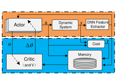
Figure 1: Overview of the L-DBAC framework.

In this paper, the actor network is instantiated as a deep neural network, specifically a three-layer multilayer perceptron. Each layer is equipped with 128 hidden units and employs the hyperbolic tangent (tanh) as the activation function. The feature extractor is another deep neural network with a similar structure of actor network, but is fine-tuned to output a reduced feature dimensionality, consisting of 10 neurons in its output layer for feature dimension reduction before forwarding to the critic. The critic itself is formulated as a Gaussian process, with a state kernel $k_{s}$ (arbitrary, we use deep RBF kernel [5]) and the Fisher kernel $k_{f}$ (indispensable) [2].

Algorithm 1 Lyapunov Deep Bayesian Actor-Critic (L-DBAC)

0:  Initial policy parameters $\bm{\theta}$, episodes for gradient evaluation $M$, termination threshold $\varepsilon$, learning rate $\beta$

1:  for $i=0$ to $M$ do

2:     for $t=0$ to $T$ do

3:        Sample $\bm{a}_{t}$ from $\bm{\pi}_{\theta}(\bm{a}_{t}|\bm{s}_{t})$ and step forward

4:        Observe $\bm{s}_{t+1}$, $c_{t}$ and store as $(\bm{s}_{t},\bm{a}_{t},c_{t},\bm{s}_{t+1},\bm{a}_{t+1})$ in $\bm{D}$

5:     end for

6:     done = false

7:     while not done do

8:        Run L-GPTD, return $\hat{\bm{\alpha}}$, $\bm{U}$ and $\bm{G}^{-1}$ with (37),(17) and (19).

9:        $\Delta{\bm{\theta}}=c_{2}\bm{G}^{-1}\bm{U}\hat{\bm{\alpha}}$

10:        $\bm{\theta}:=\bm{\theta}-\beta\Delta\bm{\theta}$ in (20)

11:        if $\Delta\bm{\theta}<\epsilon$, then done=true

12:     end while

13:  end for

14:  Return $\bm{\theta}^{*}=\bm{\theta}$

5.2 Simulated Experiments in MuJoCo

In this section, we evaluate the proposed method in three simulated robotic control tasks (i.e., Cartpole, Hopper, and Walker) via the MuJoCo physics engine [17]. Our assessment focuses on two critical dimensions:

• Performance: (1) whether the proposed training algorithm converges with random parameter initialization; (2) whether the goal of the task can be achieved, or the cumulative cost can be minimized;

• Robustness: performance of the trained policies perform when faced with uncertainties overlooked during training, such as parametric variation and external disturbances.

5.2.1 Simulation Setup

Our experimental setup adheres to the framework established in [18] except where specific modifications are introduced as described in Section 5.1. We first consider the Cartpole task, which is a classical control task [29]. The controller is expected to maintain the pole vertically at the target position $x=0$ and target angle $\phi=0$, thus the cost function is set as $c=4*(\frac{x}{x_{\text{threshold}}})^{2}+20*(\frac{\phi}{\phi_{\text{threshold}}})^{2}$ where $\phi_{\text{threshold}}$ and $x_{\text{threshold}}$ are the maximum of position and angle as in [18]. Then, we consider more complicated high-dimensional continuous control problems (i.e., Hopper and Walker) in MuJoCo. These tasks are adapted from the OpenAI Gym’s robotics environment [30], withe the goal of directing the robots to achieve a predefined target velocity. For both Hopper and Walker, the cost function is formulated as $c=(v-v_{goal})^{2}$ where $v$ is the forward velocity and $v_{goal}=$1\text{\,}\mathrm{m}\mathrm{/}\mathrm{s}$$ is the target velocity. Each task is conducted over an episode duration of 250 steps. To evaluate the performance of the policy trained by L-DBAC, we compare against DBQPG in the representative problems mentioned above with increasing complexity, where each method is trained over five random seeds with random initialization and optimized hyper-parameters listed in Table.1.

Table 1: Hyperparameter setting in RL

Hyperparameter	Cartpole	Hopper	Walker	Spacecraft
Batch size	15000	20000	15000	20000
Total episode	500	700	700	6000
Discount factor $\gamma$	0.98	0.995	0.98	0.98
$c_{1}$ (for kernel $k_{s}$)	1	1	1	1
$c_{2}$ (for kernel $k_{f}$)	$5\times 10^{-5}$	$5\times 10^{-5}$	$5\times 10^{-5}$	$5\times 10^{-5}$
Gaussian process’s noise $\sigma^{2}$	$10^{-4}$	$10^{-4}$	$10^{-4}$	$10^{-4}$

5.2.2 Performance

The cumulative control performance during training is shown in Figure. 2. In Cartpole, convergence is observed for both algorithms around the $120$ episode. Both algorithms can get a good score after $100$ episodes in Hopper. For the Walker task, convergence is achieved after approximately $500$ episodes,with DBQPG exhibiting a more gradual learning curve. Despite variations in initialization, both L-DBAC and DBQPG methods could converge at roughly the same episodes and achieve a similar result, while the DBQPG method is a bit flatter in terms of the learning curve. Crucially, the incorporation of the Lyapunov function within the L-DBAC framework does not appear to compromise performance, as evidenced by the approximate parity in cumulative costs achieved across each task when compared to DBQPG.

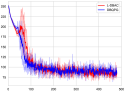
((a))

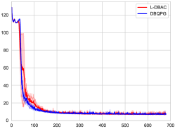
((b))

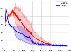
((c))

Figure 2: Cumulative control performance comparison. The Y-axis indicates the total cost during one episode, and the X-axis indicates the total episodes. The shaded region shows the 1-SD confidence interval over three random seeds. Across all trials of training, L-DBAC converges to stabilizing solution with comparable or superior performance compared with DBQPG.

5.2.3 Robustness to parametric uncertainties

To evaluate the robustness of the algorithm, we vary the system parameters in the model/simulator during the inference. In CartPole, we vary the mass of pole $m_{\text{pole}}$, and the episode ends if $|x|>10$ or $|\phi|>20^{\circ}$ and the episodes end in advance. In Hopper, we vary the length of the leg $l_{i}$. The episode ends when the height of the center of mass is greater than $0.7\text{\,}\mathrm{m}$, and the pitch angle is less than $20^{\circ}$. In Walker, we vary the ratio of calf to thigh length $\alpha_{rate}$. The episode ends when the height of the center of mass is greater than $0.8\text{\,}\mathrm{m}$ and not less than $2\text{\,}\mathrm{m}$, and the pitch angle is less than $12^{\circ}$. As shown in Figure. 3, the policies trained by L-DBAC are more robust to the dynamic uncertainties in each case compared with DBQPG. On the other hand, though DBQPG performs well in the environment without any parametric uncertainties, it is highly likely to fail when the uncertainty is great.

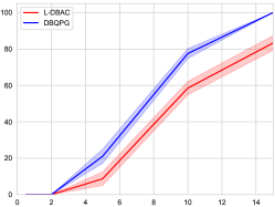
((a))

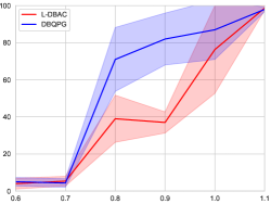
((b))

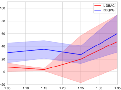
((c))

Figure 3: L-DBAC and DBQPG agents in the presence of dynamic uncertainties. The solid line indicates the average value and shadowed region for the 1-SD confidence interval. , (a) the mass of pole in CartPole, (b) the leg length in Hopper and (c) ratio of calf to thigh length in Walker varied during the inference respectively. Y-axis shows the death rate during the inference.

5.2.4 Robustness to disturbances

An inherent property of a stable system is to recover from perturbations such as those caused by external forces or environmental factors like wind. To evaluate this aspect of stability, we introduce periodic external disturbances with different magnitudes in each environment to observe the performance difference between policies trained by L-DBAC and DBQPG. Specifically, an impulsive disturbance torque is applied to each joint every $20$ step. For Cartpole, the magnitude of the disturbances ranges from $40$ to $100$ units. For Hopper and Walker, the magnitude of the disturbances ranges from $0.2$ to $2$ units. The agent may fall over when interfered with by an external force in each environment, ending the episode in advance. Therefore, we evaluate the robustness of controllers through the death rate, which is the probability of falling over after being disturbed. Under each disturbance magnitude, the policies are tested for $1000$ trials, and the performance is shown in Figure. 4(c). As shown in Figure. 4(c), the controllers trained by L-DBAC outperform DBQPG to a great extent in CartPole and Hopper. In Walker, the L-DBAC and DBQPG both perform reliably and show insensitivity to external disturbances.

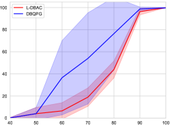
((a))

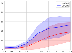
((b))

((c))

Figure 4: Performance of L-DBAC and DBQPG in the presence of persistent disturbances with different magnitudes. The X-axis indicates the mangnitude of the applied disturbance. The Y-axis indicate the death rate in each task. All of the trained policies are evaluated for 100 trials in each setting.

5.3 Real World Experiment on Proximity Maneuvers and Docking

The efficacy of our algorithm was assessed through the execution of autonomous proximity maneuvers and docking task conducted on an air-bearing testbed. Our experimental configuration draws parallels to the setup described in [31], with the notable distinction that our current focus does not encompass obstacle avoidance—a challenge we aim to address in future work. The principal objective of this experimental inquiry was to ascertain the ”sim-to-real” transferability of our method, thereby gauging its practical applicability in real-world scenarios.

5.3.1 Experiment setup

In the conducted experiment, the air-bearing testbed serves as a frictionless planar analog for space dynamics (see Figure. 5(b)). The Chaser spacecraft simulator (see Figure. 5(c)) is a designed autonomous vehicle capable of floating via air bearings and actuated by a set of eight ducted fans instead of thrusters to provide longer-lasting force and torque. The simulator is outfitted with an onboard computer featuring an Intel Core processor N2920 and 4GB of internal storage, operating under a real-time operating system. It is also equipped with fluorescent markers to facilitate the measurement of attitude and position, as well as a compressed air tank to supply the air bearings. The simulator’s physical specifications are as follows: the mass $m=$9.6\text{\,}\mathrm{k}\mathrm{g}$$, the inertia $I_{z}=$0.23\text{\,}\mathrm{k}\mathrm{g}\mathrm{m}^{2}$$, the control force $f_{max}=$1\text{\,}\mathrm{N}$$, the width $0.2\text{\,}\mathrm{m}$, and the sample interval $\Delta t=$0.05\text{\,}\mathrm{s}$$.

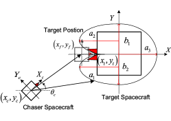
((a))

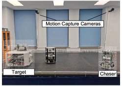
((b))

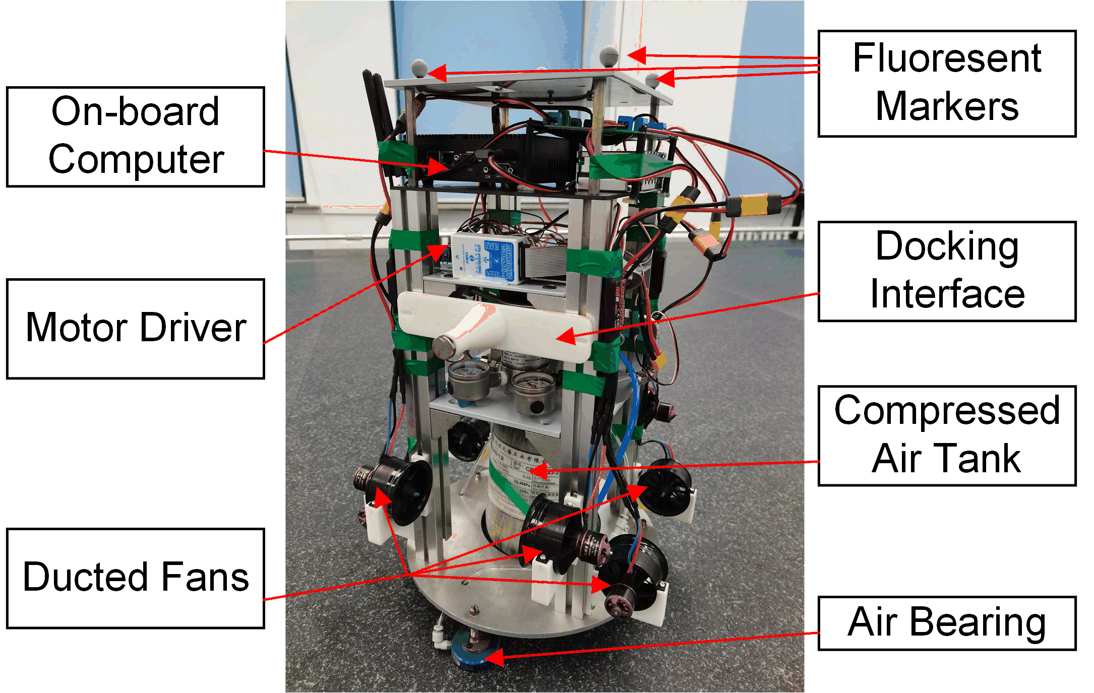
((c))

Figure 5: Proximity maneuver and docking problem setup

5.3.2 Training in simulation

We consider a planar proximity maneuver and docking task involving a Chaser spacecraft and a Target spacecraft, and Figure.5(a) illustrates the conceptual constraints of the keep-out zone. We use the same mathematical model as described in [31]. The state $\bm{s}=\left[x_{f}-x_{c},y_{f}-y_{c},\theta,\dot{x}_{f}-\dot{x}_{c},\dot{y}_{f}-\dot{y}_{c},\dot{\theta}\right]^{\top}\in\mathbb{R}^{6}$ captures the relative position and velocity with respect to the Target, and the action $\bm{a}=\left[f_{x},f_{y},\tau\right]^{\top}\in\mathbb{R}^{3}$ represents the control forces and torque. To ensure a safe final approach for docking, the docking cone boundaries are described as a cardioid-like function consisting of four ellipses, detailed in [31]. The cost function is set as $c=c_{a}+c_{b}$. The attractive function $c_{a}=\bm{x}_{fc}^{T}\bm{Q}_{a}\bm{x}_{fc}$, where $\bm{Q}_{a}>0$ is a positive definite matrix, $\bm{x}_{fc}=\bm{x}_{f}-\bm{x}_{c}$ is the relative position between the Chaser $\bm{x}_{c}$ and the Target position $\bm{x}_{f}$. The repulsive function $c_{b}=\frac{k_{r}}{2}\frac{\mathbf{x}_{fc}^{T}\bm{Q}_{b}\mathbf{x}_{fc}}{\exp\left[\mathbf{x}_{bc}^{T}\bm{P}_{b}\mathbf{x}_{bc}-1\right]}$ models the keep-out zone around the Target, with $k_{r}\in\mathbb{R}_{+}$, and $\bm{Q}_{b}$, $\bm{P}_{b}$ as positive definite matrices, where $\bm{x}_{bc}=\bm{x}_{b}-\bm{x}_{c}$ is the relative position between the Chaser $\bm{x}_{c}$ and the Target boundary constraint position $\bm{x}_{b}$. The training episode concludes when the Chaser attains the requisite proximity for docking, at which the cost $c$ is set to zero.

In the simulation, we utilize both L-DBAC and DBQPG to train the policy under identical physical parameters. Each algorithm underwent 1300 policy updates, with training conducted over five random seeds. The hyper-parameters are set as follows: $k_{r}=1.0$, $\bm{Q}_{a}=\operatorname{diag}([0.025,0.025,0.075])$, $\bm{Q}_{b}=\operatorname{diag}([0.0125,0.0125,0.175])$, $\bm{P}_{b}=\operatorname{diag}([20,20,0])$. Figure.6(a) indicates that both L-DBAC and DBQPG exhibit rapid convergence, typically within 100 episodes, starting from random parameter initializations. The total cost of L-DBAC is slightly lower than that of the DBQPG, while L-DBAC has a larger variance. Figure.6(b) shows that the average success rate for both L-DBAC and DBQPG escalates to 100% after around 100 episodes.

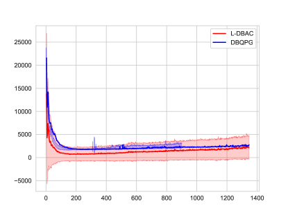
((a))

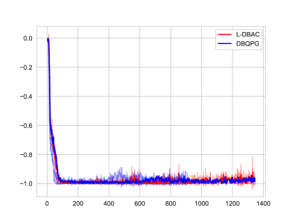
((b))

Figure 6: Performance of L-DBAC and DBQPG during the training process in simulations of proximity maneuvers and docking task

5.3.3 Air-bearing Testbed Evaluation and Analysis

After training, we directly deploy the policy learned from the simulation into the air bearing testbed in Figure.7. We tested the policies generated from 5 random seeds using DBQPG and L-DBAC algorithms, initiating from different initial positions and velocities by manual intervention. The policy formulated via DBQPG algorithm consistently failed accross across all trials. In contrast, the policy developed through L-DBAC approach demonstrated a high success rate (around 50 %), albeit not achieving universal success. Documentation of these trials, including video evidence of both triumphant and unsuccessful attempts with L-DBAC, as well as the unsuccessful endeavors with DBQPG, has been made accessible (see Supplementary Materials Movie S1).

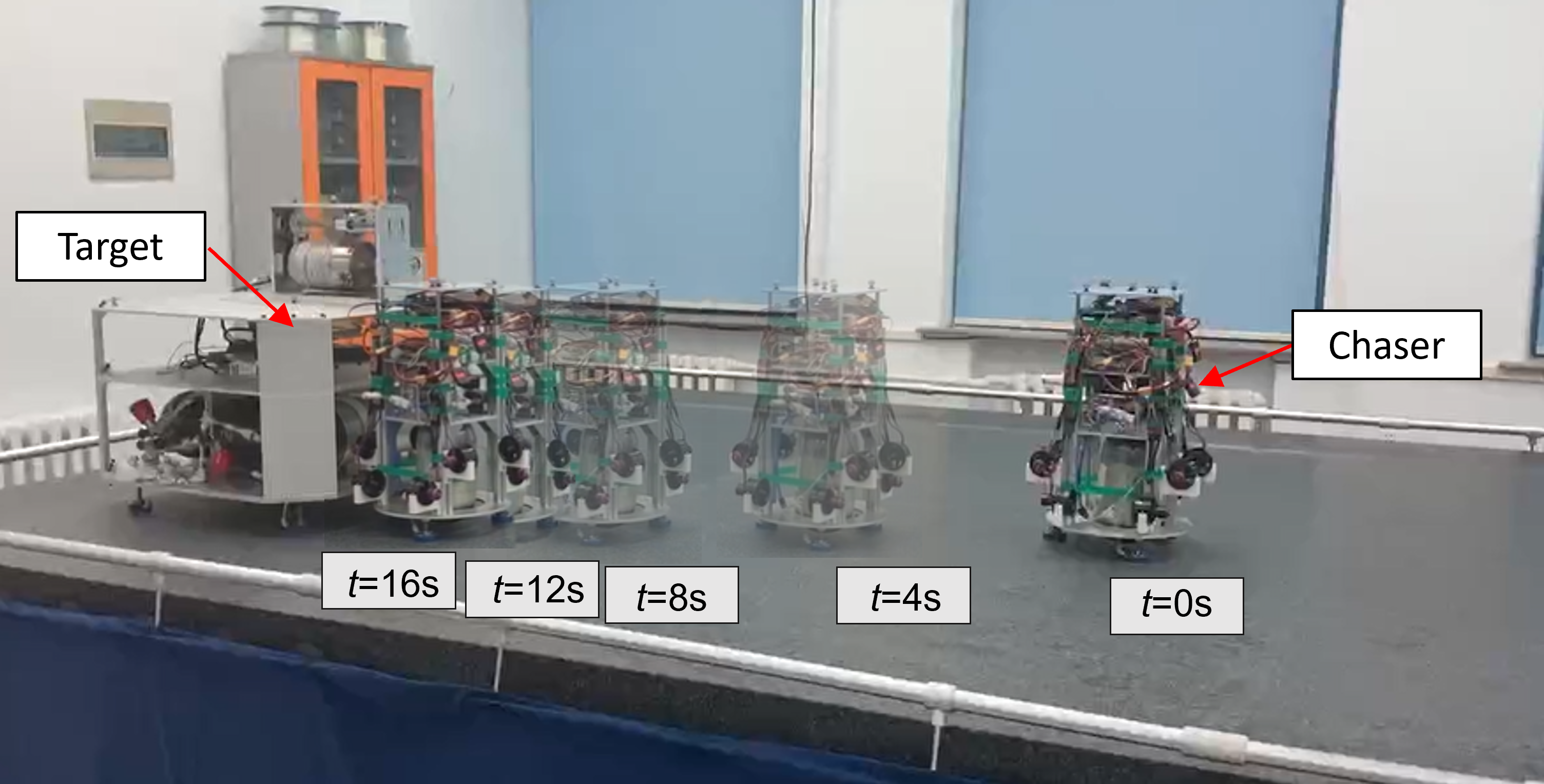
Figure 7: The trajectory of the Chaser in the air bearing testbed.

We also trained the policy using the LAC algorithm in [18], and other popular RL algorithms such as PPO [32], SAC [19] (we use the same hyperparameters as described in [18]). They showed good performance in simulation, like DBQPG and L-DBAC. However, we surprisingly found that these algorithms can not succeed either in the real world. Although we do not fully understand the reasons of failure since there are many impacting factors in the real world, we try to analyze further and draw the following possible reasons. First, the accuracy of the actuator cannot match the control command resolution and range due to the existence of the dead zone of the actuator and the nonlinearity of the actuator model. Second, the state information, especially the speed of the Chaser simulator, is much noisier than expected. There may exist some other factors that we have not found yet or are not critical. A potential future work would be to identify the accurate model of the Chaser spacecraft and combine it with model-based control and RL approaches.

6 CONCLUSIONS and DISCUSSIONS

This paper propose a deep Bayesian actor-critic reinforcement learning method to learn a control policy for robotic systems modeled by Markov decision process. We take inspiration from Lyapunov theory to ensure the closed-loop system with stability guarantee with the learned policy. We evaluate the proposed method in various simulated examples and show that our method achieves comparable performance and outperforms impressively in terms of robustness to uncertainties such as model parameter variations and external disturbances. We also evaluate our method’s sim-to-real capability on a real-world autonomous spacecraft proximity maneuvers and docking experiment on an air-bearing testbed.

Supplementary Materials

Describe any supplementary materials submitted with the manuscript (e.g., audio files, video clips or datasets). Movie S1. Simulation_Cartpole_Hpooer_Wlaker.mp4 shows the L-DBAC’s performance in these simulated robotic control tasks in MuJoCo. Movie S2. BRL with lyapunov functions proors.mp4 shows the performance of the L-DBAC and DBQPG algorithms on proximity maneuver and docking task in an air bearing testbed.

References

• [1] Richard S Sutton and Andrew G Barto “Reinforcement learning: An introduction” MIT press, 2018
• [2] Mohammad Ghavamzadeh, Shie Mannor, Joelle Pineau and Aviv Tamar “Bayesian reinforcement learning: A survey” In Foundations and Trends in Machine Learning, 2015
• [3] Yaakov Engel, Shie Mannor and Ron Meir “Bayes meets Bellman: The Gaussian process approach to temporal difference learning” In Proceedings of the 20th International Conference on Machine Learning, 2003, pp. 154–161
• [4] Yaakov Engel, Shie Mannor and Ron Meir “Reinforcement learning with Gaussian processes” In Proceedings of the 22nd International Conference on Machine Learning, 2005, pp. 201–208
• [5] Andrew Gordon Wilson, Zhiting Hu, Ruslan Salakhutdinov and Eric P Xing “Deep kernel learning” In Artificial intelligence and statistics, 2016, pp. 370–378 PMLR
• [6] Mohammad Ghavamzadeh and Yaakov Engel “Bayesian actor-critic algorithms” In Proceedings of the 24th International Conference on Machine Learning, 2007, pp. 297–304
• [7] Anthony O’Hagan “Bayes–hermite quadrature” In Journal of statistical planning and inference 29.3 Elsevier, 1991, pp. 245–260
• [8] Philipp Hennig, Michael A Osborne and Mark Girolami “Probabilistic numerics and uncertainty in computations” In Proceedings of the Royal Society A: Mathematical, Physical and Engineering Sciences 471.2179 The Royal Society Publishing, 2015, pp. 20150142
• [9] Ravi Tej Akella et al. “Deep Bayesian Quadrature Policy Optimization” In Proceedings of the AAAI conference on artificial intelligence 35.8, 2021, pp. 6600–6608
• [10] Mathukumalli Vidyasagar “Nonlinear systems analysis” SIAM, 2002
• [11] Aleksandr Mikhailovich Lyapunov “The general problem of the stability of motion” In Annals of Mathematics Studies, 1892
• [12] Felix Berkenkamp, Matteo Turchetta, Angela Schoellig and Andreas Krause “Safe model-based reinforcement learning with stability guarantees” In Advances in neural information processing systems 30, 2017
• [13] Ya-Chien Chang, Nima Roohi and Sicun Gao “Neural lyapunov control” In Advances in neural information processing systems 32, 2019
• [14] Spencer M. Richards, Felix Berkenkamp and Andreas Krause “The Lyapunov Neural Network: Adaptive Stability Certification for Safe Learning of Dynamical Systems” In Proceedings of The 2nd Conference on Robot Learning 87, Proceedings of Machine Learning Research PMLR, 2018, pp. 466–476
• [15] Wanxin Jin, Zhaoran Wang, Zhuoran Yang and Shaoshuai Mou “Neural certificates for safe control policies” In arXiv preprint arXiv:2006.08465, 2020
• [16] Charles Dawson, Zengyi Qin, Sicun Gao and Chuchu Fan “Safe nonlinear control using robust neural lyapunov-barrier functions” In Conference on Robot Learning, 2022, pp. 1724–1735 PMLR
• [17] Emanuel Todorov, Tom Erez and Yuval Tassa “Mujoco: A physics engine for model-based control” In 2012 IEEE/RSJ International conference on Intelligent Robots and Systems, 2012, pp. 5026–5033 IEEE
• [18] Minghao Han, Lixian Zhang, Jun Wang and Wei Pan “Actor-critic reinforcement learning for control with stability guarantee” In IEEE Robotics and Automation Letters 5.4 IEEE, 2020, pp. 6217–6224
• [19] Tuomas Haarnoja, Aurick Zhou, Pieter Abbeel and Sergey Levine “Soft actor-critic: Off-policy maximum entropy deep reinforcement learning with a stochastic actor” In Proceedings of the 35th International Conference on Machine Learning, 2018, pp. 1861–1870 PMLR
• [20] Vladimir I Vorotnikov “Partial stability and control: The state-of-the-art and development prospects” In Automation and Remote Control 66.4 Springer, 2005, pp. 511–561
• [21] Hassan K Khalil “Nonlinear Systems” In Patience Hall 115, 2002
• [22] Richard S Sutton, David McAllester, Satinder Singh and Yishay Mansour “Policy gradient methods for reinforcement learning with function approximation” In Advances in neural information processing systems 12, 1999
• [23] Carl Edward Rasmussen “Gaussian processes in machine learning” In Summer school on machine learning, 2003, pp. 63–71 Springer
• [24] Seung-Jean Kim, Kwangmoo Koh, Stephen Boyd and Dimitry Gorinevsky $\backslash$ell_1 trend filtering” In SIAM review 51.2 SIAM, 2009, pp. 339–360
• [25] Christian Agrell “Gaussian processes with linear operator inequality constraints” In Journal of Machine Learning Research, 2019
• [26] Laura P Swiler et al. “A survey of constrained Gaussian process regression: Approaches and implementation challenges” In Journal of Machine Learning for Modeling and Computing 1.2 Begel House Inc., 2020
• [27] Jacob Gardner et al. “Gpytorch: Blackbox matrix-matrix gaussian process inference with gpu acceleration” In Advances in neural information processing systems 31, 2018
• [28] John Schulman et al. “Trust region policy optimization” In Proceedings of the 32nd International Conference on Machine Learning, 2015, pp. 1889–1897 PMLR
• [29] Andrew G Barto, Richard S Sutton and Charles W Anderson “Neuronlike adaptive elements that can solve difficult learning control problems” In IEEE Transactions on Systems, Man, and Cybernetics IEEE, 1983, pp. 834–846
• [30] Greg Brockman et al. “Openai gym” In arXiv preprint arXiv:1606.01540, 2016
• [31] Richard et al. “Real Time Autonomous Spacecraft Proximity Maneuvers and Docking Using an Adaptive Artificial Potential Field Approach” In IEEE Transactions on Control Systems Technology 27.6, 2018, pp. 2598–2605
• [32] John Schulman et al. “Proximal policy optimization algorithms” In arXiv preprint arXiv:1707.06347, 2017