High-Order Harmonic Generation in Helium: A Comparison Study

Abstract

We report a detailed study of high-order harmonic generation (HHG) in helium. When comparing predictions from a single-active-electron model with those from all-electron simulations, such as ATTOMESA and $R$-matrix with time-dependence, which can include different numbers of states in the close-coupling expansion, it seems imperative to generate absolute numbers for the HHG spectrum in a well-defined framework. While qualitative agreement in the overall frequency dependence of the spectrum, including the cut-off frequency predicted by a semi-classical model, can be achieved by many models in arbitrary units, only absolute numbers can be used for benchmark comparisons between different approaches.

I Introduction

High-order harmonic generation (HHG) is an important method to generate coherent soft X-rays by producing odd harmonics of a fundamental frequency from an intense few-pulse laser, often with a frequency in the mid-infrared range Rothhardt et al. (2014); Stein et al. (2016); Li et al. (2017). Over the past four decades, numerous experimental and theoretical papers have been published on the subject – too many to produce a representative and unbiased reference selection of even moderate size. Most studies fall into two categories: the generation of attosecond pulses using HHG Chini et al. (2014), and the use of HHG as a measurement tool Smirnova and Gessner (2013); Corkum (2011). The most common means of understanding the HHG process is based on the semi-classical “three-step model” introduced by Schafer et al. Schafer et al. (1993) and Corkum Corkum (1993), which explains some of the basic characteristics of the process and its observations. In that model, after an electron escapes from the target by tunnel ionization, it is driven further away by the strong electric field, until it is finally accelerated back towards its parent ion upon reversal of the field. During the recollision process, some of the electron’s energy is released as a high-energy photon whose frequency must be an odd multiple of the fundamental frequency of the driving field. The process repeats for various cycles of the driving laser field. Due to the exponential dependence of the tunnel probability on the width of the barrier, which in turn is determined by the field strength, the largest effects occur near the peak amplitude of the field.

From the above model, one can estimate the maximum photon energy, or cutoff energy, that is producible by HHG from a single laser source. This cutoff energy is given by Corkum (1993)

$$E_{\rm c}=I_{p}+3.17\,U_{p},$$ (1)

where $I_{p}$ is the atomic ionization potential and $U_{p}$ is the ponderomotive potential. The latter can be approximated in terms of the laser peak intensity and wavelength as

$$U_{p}=\frac{2\,e^{2}}{c\,\epsilon_{0}\,m}\;\frac{I_{0}\,\lambda^{2}}{16\,\pi^{2}}.$$ (2)

Here $e$ is the electron charge, $c$ the speed of light, $\epsilon_{0}$ the vacuum permittivity, $m$ the electron mass, $I_{0}$ the laser peak intensity, and $\lambda$ the (central) wavelength of the driving laser.

Interestingly, the vast majority of papers on the topic of HHG present the spectrum in “arbitrary units”. While this might be the only option for experimental studies due to the notorious difficulties associated with absolute intensity measurements, all the relevant quantities are well defined. Even though different definitions (see below) are used by individual groups, presenting theoretical HHG spectra with an absolute unit is certainly possible. The quantity generally agreed upon as being the determining factor for the HHG spectrum is the dipole moment that is induced in the system by the external driving field. In particular, we are interested in the Fourier transform of the dipole acceleration, i.e.,

$$\tilde{a}(\omega)=\int_{-\infty}^{+\infty}a(t)\,{\rm e}^{i\omega t}dt,$$ (3)

where $a(t)$ is the second derivative with respect to time of the induced dipole moment $d(t)$.

The present work is a follow-up on our recent study Finger et al. (2022) of HHG in neon, where we looked at the particularly challenging problem of reaching the so-called “water window” of HHG frequencies ranging from the $K$-absorption edge of carbon to the $K$-edge of oxygen. In order to do so, we compared results from a single-active-electron (SAE) model with predictions from the $R$-matrix with time-dependence (RMT) Brown et al. (2020) approach. The latter is implemented in a general all-electron code based on the close-coupling formalism. As such, electron exchange and correlation effects are accounted for in RMT, whereas they are neglected in SAE.

While there was qualitative agreement between the SAE and RMT results, it was difficult to explain the remaining quantitative differences, which were only found due to the fact that we chose to compare absolute numbers using the formula

$$S(\omega)\!=\!\frac{2}{3\pi c^{3}}\,|\tilde{a}(\omega)|^{2}$$ (4)

for the so-called “spectral density” $S(\omega)$ Joachain et al. (2012); Telnov et al. (2013). We will refer to the above equation as the “acceleration form”. We also investigated equivalent formulas using the dipole moment directly (the “length form”) or its first time derivative (the “velocity form”). In addition to the order of the time differentiations, the formulas differ by factors of $\omega^{2}$ and $\omega^{4}$ arising from transforming to the velocity and length forms, respectively. As a numerical check, we verified that the results from the three methods agree well with one another, although the spectra are not exactly equivalent due to additional terms that may be present after the pulse has vanished (see Eq. (22) of Guan et al. (2006)). All of the results in this paper are presented in the acceleration form. We emphasize again that the pre-factor in the above equation, whose numerical value is approximately $8.25\times 10^{-8}$ in atomic units together with the definition in Eq. (3), provides an absolute value for the quantity of interest. Unless indicated otherwise, atomic units ($\hbar\!=\!e=\!m\!=\!1$; $c\!\approx\!137$), are used throughout this manuscript.

As mentioned above, other authors use different definitions. Specifically, we note the papers by Tong and Chu Tong and Chu (2001) and Guan et al. Guan et al. (2006) who defined their spectrum by

$$P(\omega)\!=\!\frac{1}{\omega^{4}\tau^{2}}\,|\tilde{a}(\omega)|^{2},$$ (5)

where $\tau$ is the length of the pulse. The authors used a fixed number of cycles with a $\sin^{2}$ envelope for the electric field. In this case, the pulse length $\tau$ from the very beginning to the very end is well defined, in contrast to somewhat more realistic pulses, e.g., a Gaussian envelope, where one usually defines the length via the full-width at half-maximum of the intensity. Normalizing to the pulse length has the advantage that pulses with a different number of cycles can be better compared with respect to the yield. Note, however, that the frequency dependence is very different in the two definitions, since the factor $1/\omega^{4}$ now appears in the acceleration form of Refs. Tong and Chu (2001) and Guan et al. Guan et al. (2006).

To simplify matters in calculating absolute HHG spectra, we decided to perform a comparison study using helium rather than the much more complex neon target. In this case, one might expect the SAE and RMT results to agree reasonably well, especially if the RMT model only includes a single target state, namely He${}^{+}(1s)$. This corresponds effectively to the “static exchange” approximation for electron scattering from He⁺. In the static exchange model, we also added results from a new multi-electron time-dependent code, ATTOMESA, to give us an additional source of comparison. We emphasize that our calculations, like many other theoretical attempts, are single-atom simulations. While they are important in practical realizations of the HHG process, we are not concerned with macroscopic effects such as phase matching or volume averaging of the intensity in the present work. We note, however, that work in this direction using the RMT code was recently reported Hutcheson et al. (2023).

Furthermore, it is possible to systematically test the effects of extending the close-coupling model by including more states, such as the $n=2$ and $n=3$ states of He⁺. Such models should indicate the importance of channel coupling as well as correlations in the initial state, whose expansion then includes doubly-excited states.

This manuscript is organized as follows. In section II, we briefly describe the SAE, RMT, and ATTOMESA models used in the present work. This is followed by the presentation and discussion of our results for two wavelengths, 248.6 nm and 1,064 nm. Since these are the wavelengths investigated by Tong and Chu Tong and Chu (2001) and Guan et al. Guan et al. (2006), we selected them and the intensities chosen in the latter studies to have a further basis for comparison with other works. As will become clear below, some of these laser parameters appear to be quite challenging from a numerical perspective. Consequently, we judge them to be a good start for benchmark studies, even though their Keldysh parameters are not in the predominantly tunneling regime.

As will be shown below, the quantitative calculation of HHG spectra is by no means trivial, due to the well-known fact that the conversion efficiency of the process is often very low. Most of the emitted radiation may simply come back at the fundamental frequency, although the choice of laser parameters (if available in the setup) can change this. Even though 248.6 nm is not a particularly suitable wavelength for HHG in practice, the calculation in Ref. Guan et al. (2006) was performed with a sophisticated two-electron code specifically designed for the helium target. These benchmark results, fortunately also given as absolute numbers, provide an excellent further source of comparison. In the spirit of the Phys. Rev. A Editorial Editors (2011), such a thorough test is highly desirable to assess the reliability of all the results presented here, as well as those from other approaches, for longer wavelengths and higher intensities.

II Theory

Since the SAE and RMT methods have been described in previous papers, we limit ourselves to a brief summary and the specifics of their applications to the helium target. We also add a short description of the ATTOMESA code, which is currently under development.

II.1 The SAE model

We employed the same SAE model as Birk et al. Birk et al. (2020) and Meister et al. Meister et al. (2020). Specifically, we used the one-electron potential

$$V(r)=-\frac{1}{r}-\left(\frac{1}{r}+1.3313\right)\,\exp(-3.0634\,r),$$ (6)

where $r$ is the distance from the nucleus, to calculate the valence orbitals. We used a variable radial grid with a smallest stepsize of 0.1 near the origin, gradually increasing by 5% per step up to a maximum stepsize of 0.2 to a box size of approximately 200. In this discretization, the difference between the predicted ionization potential and the excitation energies of all (1s$n\ell$) states with singlet spin character (the SAE is, of course, only concerned with the $n\ell$ orbital) up to $n\!=\!6$ and $\ell\!=\!5$ with the recommended values from the NIST database Kramida et al. (2023) is less than 0.2 eV even in the worst-case scenario.

Assuming that the driving radiation is linearly polarized, the initial state can be propagated very efficiently and accurately. We used an updated version of the code described by Douguet et al. Douguet et al. (2016). Based on many previous works using SAE approaches, we expected it to be more suitable for the helium target compared to heavier noble gases, as long as obvious two-electron correlation effects, e.g., autoionizing resonances, are not affecting the process significantly.

We then calculated the induced dipole moment as

$$d(t)=\langle z\rangle(t)=\langle\Psi(\bm{r},t)|z|\Psi(\bm{r},t)\rangle$$ (7)

during the pulse and numerically differentiated the function twice to obtain the dipole acceleration. Since there are two electrons in the $1s$ orbital of helium, the above dipole moment should be multiplied by 2 to account for the occupation number Tong and Chu (2001).

II.2 RMT

As a second method, we employed the general $R$-matrix with time-dependence (RMT) method Brown et al. (2020). RMT has been applied to the study of HHG several times, including HHG from two-color fields Hamilton et al. (2017), XUV-initiated HHG Brown and van der Hart (2016), and HHG from mid-IR lasers Hassouneh et al. (2014); Finger et al. (2022). Most recently, it has been extended to include macroscopic propagation effects in HHG Hutcheson et al. (2023).

To calculate the necessary time-independent basis functions and dipole matrix elements for the present work, we started with the simplest possible model, namely a nonrelativistic 1-state approach. This model, labeled RMT-1st below, is the one most closely related to the SAE approach. It essentially describes electron collisions with He⁺ in the ionic ground state. Nevertheless, there are some subtle differences, for example in the $1s$ orbital used in the two models. In the SAE, the potential given in Eq. (6) supports bound states, and the $1s$ orbital obtained that way is close to the Hartree-Fock orbital of the ground-state configuration. Since the potential used in the SAE calculations, given in Eq. (6), is not ab initio, the resulting ground-state energy of $-2.910$ is slightly lower than obtained in nonrelativistic variational calculations Drake (2023). In RMT, on the other hand, we use the analytically known $1s$ orbital of He⁺. While this is not optimal to obtain the best ground-state energy, it is a suitable orbital to describe essentially all excited states of neutral helium, which are automatically contained (to a very high accuracy) in the close-coupling approach, as long as the state fits into the $R$-matrix box.

In addition to RMT-1st, we set up two more models, one where we added the $n\!=\!2$ states of He⁺ using the $2s$ and $2p$ ionic orbitals and another one where we also included the $n\!=\!3$ states. These two models will be referred to as RMT-3st and RMT-6st, respectively. We used an $R$-matrix radius of 40.0 and 60 $B$-splines to expand the continuum orbitals inside the $R$-matrix box. Partial waves up to a total orbital angular momentum of 49 were used to ensure converged results for all cases reported below. Since we noticed a few surprising results, to be discussed in the next section, we varied the size of the $R$-matrix box, the number of splines, the number of partial waves, as well as the radial grid and the time step. We even altered the numerical accuracy of the real variables in the computer code. The results reported below did not change significantly. They were obtained with 60 splines employed to expand the one-electron orbitals inside the $R$-matrix radius of 40 and an outer-region size of about 8,000. The results did not change significantly whether or not an absorbing boundary condition was applied near the outer edge.

II.3 ATTOMESA

As a third method, we employ ATTOMESA, a new time-dependent multi-electron code for applications in attosecond science, in particular for the treatment of atoms and molecules in intense fields. In this work, we present the first results of ATTOMESA and will limit our discussion to its most salient features. The complete description of the method will be provided in a forthcoming communication.

In ATTOMESA, short-range electron exchange and correlations are described from a set of orbitals constructed from Gaussian-type orbitals (GTOs). The latter space is augmented with finite-element discrete variable (FEDVR) functions Rescigno and McCurdy (2000), which are orthogonalized to all GTOs. They describe a scattering electron and a residual correlated ion in different possible excited electronic states. Electronic integrals involving FEDVRs and GTOs are computed through the Becke integration scheme Becke (1988); Gharibnejad et al. (2021) in the inner region defined by the extension of the GTOs. Beyond this region, the photoelectron dynamics are described only by FEDVRs. Electronic integrals are computed in a single-center grid using the Gauss-Lobatto quadrature Rescigno and McCurdy (2000), taking advantage of the unique properties of the FEDVRs, such as the trivial representation of any local operator. In particular, this method leads to an extremely sparse atom-field interaction Hamiltonian in the length gauge and thereby enables the construction of efficient time-propagation schemes. The exponential time propagator is further split into field-free and atom-field interaction operators, where the action of the field-free Hamiltonian is considered in its diagonal representation, while the atom-field interaction is expressed in the FEDVR representation.

The results of ATTOMESA were benchmarked against SAE predictions for HHG from atomic hydrogen with a hybrid Gaussian-FEDVR basis set in ATTOMESA. Virtually perfect agreement was found between both methods, thereby validating the computation of the electronic integrals and the time-propagation method employed in ATTOMESA. In addition, the energies of excited Rydberg states of hydrogen (up to $n=15$) were reproduced to ten-digit accuracy. On the other hand, ATTOMESA is still under development. The calculation of the integrals can be drastically improved, and parallel-processing capabilities are not yet supported. For this reason, we are still limited in the parameter space where ATTOMESA can be applied. Therefore, calculations were only performed for the shorter wavelength and lower-intensity pulses considered in this study. The principal goal was to assess the consistency between different methods and models.

In our calculations, we use the helium cc-pVQZ basis set Woon and Dunning, Jr (1994) and construct our reference space from the first $s$ and $p$ orbitals obtained from a Hartree-Fock calculation for He. This space is complemented with the $1s$ orbital of He⁺. We obtained the He ground state energy as $-2.900$ and virtually the exact He⁺ ground-state energy of $-2.0$. We use a total box size of 300, with a complex absorbing potential (CAP) placed near the edge, and elements of radial size 10 with ten DVRs per element. For the present work, we only performed static exchange (one-state) calculations with ATTOMESA. The largest angular momentum included in the time propagation was $\ell=15$.

III Results and Discussion

We now discuss our results for two wavelengths. The first one (248.6 nm) was chosen by Guan et al. Guan et al. (2006) using a sophisticated computer code specifically designed for the two-electron helium target. Due to the complexity of the model and the available computational resources at the time, the wavelength and pulse duration were chosen relatively short in order to produce benchmark results.

The second wavelength (1,064 nm) was chosen by Tong and Chu Tong and Chu (2001), but with an SAE potential generated via density-functional theory. Hence, comparing with their results serves as an indicator for the sensitivity of the predictions to the potential employed in the SAE calculation. Most importantly, however, in light of the rapid developments in computational power, we could employ the RMT model also for this more challenging wavelength and longer pulses.

III.1 248.6 nm Driving Field

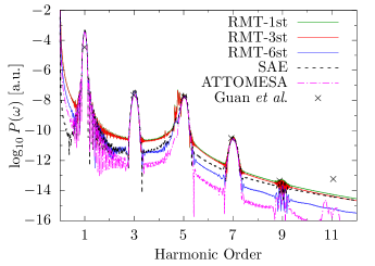
Figure 1: Spectrum for a 15-cycle pulse of central wavelength 248.6 nm with a sin² envelope of the electric field and peak intensity of $1\times\rm 10^{14}\,W/cm^{2}$. The results from our SAE model are compared with predictions from ATTOMESA and three RMT calculations with a different number of coupled states. The predicted cut-off energy from the three-step model is $\approx 26\,$eV, corresponding to the 5${}^{\rm th}\,$harmonic. The crosses are the results for the peak values obtained by Guan et al. Guan et al. (2006) in the acceleration form.

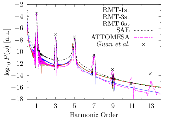
Figure 2: Spectrum for a 30-cycle pulse of central wavelength 248.6 nm with a sin² envelope of the electric field and peak intensity of $1\times\rm 10^{14}\,W/cm^{2}$.

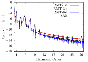
Figure 3: Spectrum for a 30-cycle pulse of central wavelength 248.6 nm with a $\sin^{2}$ envelope of the electric field and peak intensity of $5\times\rm 10^{14}\,W/cm^{2}$. The predicted cut-off energy from the three-step model is $\approx\,34\,$eV, corresponding to the 7${}^{\rm th}\,$harmonic.

Figures 1 – 3 show the HHG spectrum for 248.6 nm, using the style of Guan et al. Guan et al. (2006). Unfortunately, their results are not available in numerical form. We digitized their data, but an additional curve would make the figure practically unreadable. However, a close visual inspection shows good agreement in the main features produced by all numerical methods, i.e., the heights of the fundamental peak and of the first few harmonics. The exception is the height of the fundamental peak of Guan et al. in Fig. 1, where their result in the acceleration form seems to lie significantly below that obtained in the length form. The latter agrees well with our predictions (see their Fig. 5).

Nevertheless, there are several observations worth commenting on. To begin with, the RMT-1st and RMT-3st results are very similar. However mainly at the minima between the peaks, the results from the other models differ, with the SAE numbers close but certainly not identical to those from RMT-1st and RMT-3st, while the RMT-6st results are significantly different. Upon further analysis, we confirmed that the main reason for the change from RMT-3st to RMT-6st is the inclusion of the He${}^{+}(3p)$ state in the close-coupling expansion.

As mentioned above, we performed exhaustive tests to check the numerical accuracy of the results. None of the changes made in the numerical treatment altered the numbers for the dipole moments, and subsequently the resulting harmonic spectra, significantly. Since the dipole moment is the underlying physical quantity that determines the spectrum, and it apparently converges well against changes in the model (see also the discussion in the next section), we do believe that the basic physics is contained in our treatment. The quantitative calculation of the HHG spectrum, on the other hand, presents a surprisingly difficult task.

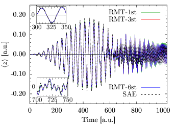
Figure 4: Dipole expectation value as a function of time for a 30-cycle pulse of central wavelength 248.6 nm with a sin² envelope of the electric field and peak intensity of $5\times\rm 10^{14}\,W/cm^{2}$ (same laser parameters as Fig. 3).

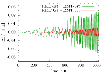
Figure 5: Difference between the dipole expectation values obtained with the RMT-1st and RMT-6st models relative to the results obtained with RMT-3st as a function of time for the laser parameters used to produce Fig. 3 (30-cycle pulse of central wavelength 248.6 nm with a sin² envelope of the electric field and peak intensity of $5\times\rm 10^{14}\,W/cm^{2}$).

Even though RMT also accounts for two-electron correlation effects, we do not see the additional high-order harmonics shown by Guan et al. Guan et al. (2006). These authors suggested correlation as the principal reason for the appearance of these additional high frequencies. Interestingly, ATTOMESA also predicts some additional structures at the high harmonics, although the heights of the predicted peaks differ significantly from those of Ref. Guan et al. (2006). These high frequencies are well suppressed in our SAE results.

As explained above, ATTOMESA cannot yet describe processes for the high-intensity and long pulses used in Fig. 3. The remaining part of this paper is, therefore, devoted to a further analysis of the various RMT predictions.

In the interest of benchmarking and testing computer codes, it is interesting to look at the quantity that actually determines the HHG spectrum, independent of how one might define it. As an example, Fig. 4 shows the induced dipole moment for the spectrum exhibited in Fig. 3. Once again, there are several interesting observations to be made. First of all, it is very difficult to see differences in the dipole expectation value predicted by the various models. This is due to the fact that the fundamental frequency is very dominant, i.e., all the higher harmonics are due to tiny differences from the dipole moment adiabatically following the driving field.

We therefore exhibit the differences between the dipole expectation values calculated within the various models in Fig. 5. As seen there, the maximum deviations in the predicted induced dipole moment by the RMT-1st and RMT-6st from the RMT-3st numbers (which we selected as the reference) are more than an order of magnitude smaller than the values of the dipole moment themselves. This already suggests that the latter must be calculated to very high accuracy in order to obtain reliable absolute values for the HHG spectrum.

A second feature of interest concerns the development of the dipole moment shortly after the maximum amplitude of the driving field. The regular structure seen up to then suddenly becomes very irregular, and the dipole moment certainly does not go back to (near) zero at the end of the pulse. In fact, the oscillations occur with a much higher frequency than that provided by the driver. We analyzed this behavior and noticed that it is due to a remaining small (a few percent) occupation of the He$\,(1s2p)^{1}P^{o}$ state. The excitation energy is between 4 and 5 driving photon energies above the ground state. Nevertheless, at the end of the pulse, the system is essentially in a coherent superposition of the ground state and the He$\,(1s2p)^{1}P^{o}$ state, with small additions from other excited bound states. As a result, we see oscillations with a frequency corresponding to the energy difference between these two states. A close inspection of the spectra exhibited in Figs. 1 – 3 reveals that these oscillations indeed affect the appearance of the spectra near the 5^th harmonic, where some additional structures can be seen.

In our previous paper Finger et al. (2022), we discussed the effect of using windows to numerically force the induced dipole moment to zero at the end of the pulse. The above discussion shows that this will not only affect, once again, the absolute values and the details of the spectrum, but it is in fact unphysical.

III.2 1,064 nm Driving Field

Figures 6 and 7 show the HHG spectrum for a 60-cycle pulse with a central wavelength of 1,064 nm and a sin² envelope of the electric field with a peak intensity of $\rm 5\times 10^{13}\,W/cm^{2}$. This is one of the cases reported by Tong and Chu Tong and Chu (2001). In contrast to the spectra shown in the previous section, the ones exhibited in Fig. 6 no longer diverge at very small frequencies due to the $1/\omega^{4}$ in their definition. Nevertheless, we also show the spectral density in Fig. 7 after evaluating it according to Eq. (4).

Once again, the RMT-6st results are significantly different than those obtained in the other models. In particular, the height of the plateau is significantly different in the RMT-6st calculation compared to the other models. The fraction of the harmonic spectra under the first few odd harmonics and the aforementioned plateau is summarized in Table 1 below.

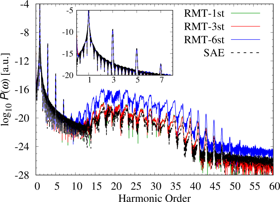
Figure 6: Spectrum for a 60-cycle pulse of central wavelength 1,064 nm with a sin² envelope of the electric field and peak intensity of $\rm 5\times 10^{13}\,W/cm^{2}$. The results from the SAE model are compared with predictions from three RMT calculations with a different number of coupled states. The predicted cut-off energy from the three-step model is $\approx\,41\,$eV, corresponding to the 35${}^{\rm th}\,$harmonic.

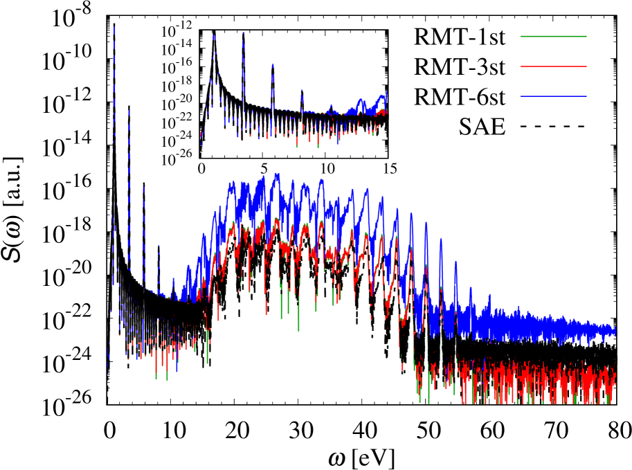
Figure 7: Spectral density as defined in Refs. Joachain et al. (2012); Telnov et al. (2013) for a 60-cycle pulse of central wavelength 1,064 nm with a sin² envelope of the electric field and peak intensity of $\rm 5\times 10^{13}\,W/cm^{2}$ (the parameters of Fig. 6). The $y$-axis is logarithmic.

To further illustrate the numerical challenges associated with an accurate calculation of the spectrum, we show in Fig. 8 the induced dipole moment for this case and in Fig. 9 the differences in the models relative to the RMT-1st result. The situation is similar, but even more pronounced, to what we saw for the 248.6 nm case: a tiny difference in the calculated dipole moment can change the predicted height of the plateau by several orders of magnitude.

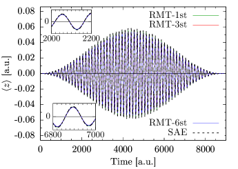
Figure 8: Dipole expectation value as a function of time for a 60-cycle pulse of central wavelength 1,064 nm with a sin² envelope of the electric field and peak intensity of $\rm 5\times 10^{13}\,W/cm^{2}$ (the parameters used to produce Fig. 6).

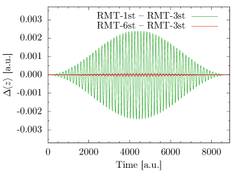
Figure 9: Difference between the dipole expectation values obtained with the RMT-1st and RMT-6st models relative to the results obtained with RMT-3st as a function of time for the laser parameters used to produce Fig. 6 (central wavelength 1,064 nm with a sin² envelope of the electric field and peak intensity of $\rm 5\times 10^{13}\,W/cm^{2}$).

Having seen that the differences in the dipole moment, as small as they are, are still large enough to result in significantly different HHG spectra, we decided to investigate how much of the induced dipole moment with the laser parameters of Fig. 6 is actually associated with the plateau of the spectrum. We did this by applying a Super-Gauss window function

$$W(\omega)\equiv{\rm e}^{-\{(\omega-\omega_{\rm c})/\omega_{\rm w}\}^{6}},$$ (8)

where $\omega_{\rm c}$ is the central frequency and $\omega_{\rm w}$ is the width, to the Fourier transform of the dipole moment and then calculating the inverse transform. We centered the function around 33 eV and chose widths of 22 eV and 14 eV, respectively. These functions are depicted in Fig. 10. We chose a linear scale on purpose to demonstrate how an apparent “zero” can be misleading.

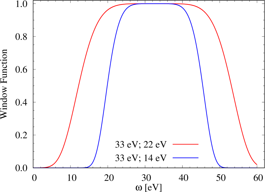
Figure 10: Super-Gauss window function centered on the plateau with different widths to focus on the frequencies of the plateau in Fig. 6.

Figure 11 shows the reconstructed dipole moment with the window function. Using the wider function, the dipole moment is reduced by four orders of magnitude, but it is still dominated by the fundamental frequency. Consequently, even though the contribution of the fundamental is drastically (but still insufficiently) reduced in the HHG spectrum, the RMT-1st and RMT-6st models still reproduce the partial dipole moment in almost the same way.

Figure 11: Reconstructed part of the dipole moment with the wider Super-Gauss window function centered on the plateau of Fig. 6.

Figure 12 shows the reconstructed dipole moment with the narrower function. Now the dipole moment is reduced by five orders of magnitude, the fundamental as well as the low-order harmonics are filtered out, and we see indeed a large difference in the reconstructed part of the dipole moment in the RMT-1st and RMT-6st models. The RMT-3st reconstruction (not shown for clarity) is very similar to that obtained from RMT-1st. While we cannot unambiguously decide that the RMT-6st results are problematic, these figures suggest that the problem is numerically ill-conditioned for this choice of parameters. For this very reason, however, we suggest it as a challenge for benchmark calculations to thoroughly test the many computer codes that have been used to predict relative rather than absolute HHG spectra.

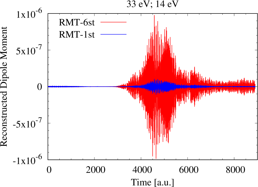
Figure 12: Reconstructed part of the dipole moment with the narrower Super-Gauss window function centered on the plateau of Fig. 6.

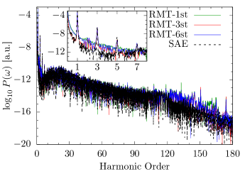
Figure 13: Same as Fig. 6 for a peak intensity of $\rm 4\times 10^{14}\,W/cm^{2}$. The predicted cut-off energy from the three-step model is $\approx\,160\,$eV, corresponding to the 137${}^{\rm th}\,$harmonic.

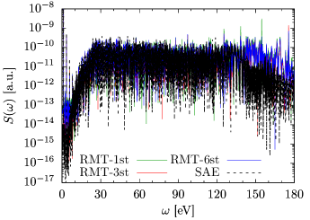
Figure 14: Spectral density as defined in Refs. Joachain et al. (2012); Telnov et al. (2013) for the laser parameters used to produce Fig. 13. The $y$-axis is logarithmic.

Our final comparison with the results of Tong and Chu Tong and Chu (2001) is shown in Fig. 13, and we again also exhibit the results obtained with Eq. (4) in Fig. 14. Even though details are hardly visible, there appears to be quantitative agreement with the results shown in Fig. 5(b) of Ref. Tong and Chu (2001).

Table 1: Fraction (in %) of the integral under various peaks in Fig. 14 for a 60-cycle pulse of central wavelength 1,064 nm with a sin² envelope of the electric field and peak intensities of $\rm Low=5\times 10^{13}\,W/cm^{2}$ and $\rm High=4\times 10^{14}\,W/cm^{2}$, respectively.

Model	SAE		RMT-1st		RMT-3st		RMT-6st
Intensity	Low	High	Low	High	Low	High	Low	High
fundamental	99.97689	9.71731	99.97233	7.61130	99.96863	9.35664	99.96643	7.81866
$3^{\rm rd}$ harmonic	0.02309	0.42943	0.02764	0.25380	0.03134	0.33415	0.03134	0.29346
$5^{\rm th}$ harmonic	0.00001	0.02763	0.00001	0.00681	0.00001	0.00859	0.00001	0.00607
plateau	$2.7\times 10^{-6}$	87.46749	0.00001	90.50232	0.00001	88.75972	0.00014	89.97512

As pointed out in Ref. Finger et al. (2022), a quantity of significant practical interest is the conversion efficiency, i.e., what portion of the incident intensity can actually be converted into a few low-order harmonics and the plateau. In fact, a straightforward indication is a comparison of the integrals under the various peaks and the plateau. Due to the likely singularity for $\omega\to 0$ in the definition of Refs. Tong and Chu (2001); Guan et al. (2006), we only use Eq. (4) to obtain the fractions relative to the integral under the entire curve.

The results are listed in Table 1. We only present them for the 1,064 nm case discussed in this subsection, since there is no real plateau for 248.6 nm. For the relatively low peak intensity of $\rm 5\times 10^{13}\,W/cm^{2}$, the spectra are completely dominated by the contribution from the fundamental frequency, followed by rapid drops for the low-order harmonics that are still distinguishable on the graphs. The relative importance of the plateau is most important according to the RMT-6st model for this low intensity. However, the numbers are extremely small, and such small numbers are usually very difficult to calculate accurately.

For the higher peak intensity of $\rm 4\times 10^{14}\,W/cm^{2}$, on the other hand, the integral under the plateau provides the dominant contribution to the spectrum. As one might expect for this case of larger numbers, the numerical challenges appear to be less significant. Table 1 shows that for the high-intensity results, the plateau integrals all agree to within about 3%, a significant improvement upon the order-of-magnitude disagreement observed in the low-intensity case. We note that the total ionization probability for the laser parameters selected for this case is still only about 0.1%, i.e., this is consistent with the usual HHG condition of almost negligible ionization.

IV Conclusions

We have reported a comparison study for high-order harmonic generation in helium. While many results for this problem have been reported previously, we emphasized the importance of a number of items that seem to have been frequently ignored in other works. Most importantly, we continue to advocate that theorists publish absolute numbers, together with the definition they used to obtain them. Furthermore, we illustrated that the induced dipole moment needs to be calculated with very high accuracy if reliable benchmark results are to be obtained, which can then be used to assess the likely reliability of the predictions.

Finally, we found a surprising effect on the results by adding the $n=3$ states (specifically the $3p$) of He⁺ into the RMT model. We hope that the present work will encourage other groups to perform calculations that, hopefully, will lead to an established benchmark result. The exact time profile of the pulses we used, as well as the numerical results for all parameters plotted in the graphs, are available upon request.

References

- Rothhardt et al. (2014) J. Rothhardt, S. Hädrich, A. Klenke, S. Demmler, A. Hoffmann, T. Gotschall, T. Eidam, M. Krebs, J. Limpert, and A. Tünnermann, Opt. Lett. 39, 5224 (2014).
- Stein et al. (2016) G. J. Stein, P. D. Keathley, P. Krogen, H. Liang, J. P. Siqueira, C.-L. Chang, C.-J. Lai, K.-H. Hong, G. M. Laurent, and F. X. Kärtner, J. Phys. B: At. Mol. Opt. Phys. 49, 155601 (2016).
- Li et al. (2017) J. Li, X. Ren, Y. Yin, K. Zhao, A. Chew, Y. Cheng, E. Cunningham, Y. Wang, S. Hu, Y. Wu, M. Chini, and Z. Chang, Nat. Commun. 8, 186 (2017).
- Chini et al. (2014) M. Chini, Z. K., and Z. Chang, Nat. Photon. 8, 178 (2014).
- Smirnova and Gessner (2013) O. Smirnova and O. Gessner, Chem. Phys. 414, 1 (2013).
- Corkum (2011) P. B. Corkum, Phys. Today 64, 36 (2011).
- Schafer et al. (1993) K. J. Schafer, B. Yang, L. F. DiMauro, and K. C. Kulander, Phys. Rev. Lett. 70, 1599 (1993).
- Corkum (1993) P. B. Corkum, Phys. Rev. Lett. 71, 1994 (1993).
- Finger et al. (2022) K. Finger, D. Atri-Schuller, N. Douguet, K. Bartschat, and K. R. Hamilton, Phys. Rev. A 106, 063113 (2022).
- Brown et al. (2020) A. C. Brown, G. S. Armstrong, J. Benda, D. D. Clarke, J. Wragg, K. R. Hamilton, Z. Mašín, J. D. Gorfinkiel, and H. W. van der Hart, Comp. Phys. Commun. 250, 107062 (2020).
- Joachain et al. (2012) C. J. Joachain, N. Kylstra, and R. M. Potvliege, Atoms in Intense Laser Fields (Cambridge University Press, 2012).
- Telnov et al. (2013) D. A. Telnov, K. E. Sosnova, E. Rozenbaum, and S.-I. Chu, Phys. Rev. A 87, 053406 (2013).
- Guan et al. (2006) X. Guan, X.-M. Tong, and S.-I. Chu, Phys. Rev. A 73, 023403 (2006).
- Tong and Chu (2001) X.-M. Tong and S.-I. Chu, Phys. Rev. A 64, 013417 (2001).
- Hutcheson et al. (2023) L. Hutcheson, H. W. van der Hart, and A. C. Brown, J. Phys. B: At. Mol. Opt. Phys. 56, 135402 (2023).
- Editors (2011) The Editors, Phys. Rev. A 83, 040001 (2011).
- Birk et al. (2020) P. Birk, V. Stooß, M. Hartmann, G. D. Borisova, A. Blättermann, T. Heldt, K. Bartschat, C. Ott, and T. Pfeifer, J. Phys. B: At. Mol. Opt. Phys. 53, 124002 (2020).
- Meister et al. (2020) S. Meister, A. Bondy, K. Schnorr, S. Augustin, H. Lindenblatt, F. Trost, X. Xie, M. Braune, R. Treusch, B. Manschwetus, N. Schirmel, H. Redlin, N. Douguet, T. Pfeifer, K. Bartschat, and R. Moshammer, Phys. Rev. A 102, 062809 (2020).
- Kramida et al. (2023) A. Kramida, Yu. Ralchenko, J. Reader, and and NIST ASD Team, NIST Atomic Spectra Database (ver. 5.10), [Online]. Available: http://physics.nist.gov/asd National Institute of Standards and Technology, Gaithersburg, MD. (2023).
- Douguet et al. (2016) N. Douguet, A. N. Grum-Grzhimailo, E. V. Gryzlova, E. I. Staroselskaya, J. Venzke, and K. Bartschat, Phys. Rev. A 93, 033402 (2016).
- Hamilton et al. (2017) K. R. Hamilton, H. W. van der Hart, and A. C. Brown, Phys. Rev. A 95, 013408 (2017).
- Brown and van der Hart (2016) A. C. Brown and H. W. van der Hart, Phys. Rev. Lett. 117, 093201 (2016).
- Hassouneh et al. (2014) O. Hassouneh, A. C. Brown, and H. W. van der Hart, Phys. Rev. A 90, 043418 (2014).
- Drake (2023) G. W. F. Drake, Springer Handbook of Atomic, Molecular, and Optical Physics, 2nd ed., edited by G. W. F. Drake (Springer Nature, New York, NY, 2023) pp. 199–216.
- Rescigno and McCurdy (2000) T. N. Rescigno and C. W. McCurdy, Phys. Rev. A 62, 032706 (2000).
- Becke (1988) A. D. Becke, J. Chem. Phys. 88, 2547 (1988).
- Gharibnejad et al. (2021) H. Gharibnejad, N. Douguet, B. Schneider, J. Olsen, and L. Argenti, Comp. Phys. Commun. 263, 107889 (2021).
- Woon and Dunning, Jr (1994) D. E. Woon and T. H. Dunning, Jr, J. Chem. Phys. 100, 2975 (1994).