The Linear Representation Hypothesis and
the Geometry of Large Language Models

Abstract

Informally, the ‘linear representation hypothesis’ is the idea that high-level concepts are represented linearly as directions in some representation space. In this paper, we address two closely related questions: What does “linear representation” actually mean? And, how do we make sense of geometric notions (e.g., cosine similarity or projection) in the representation space? To answer these, we use the language of counterfactuals to give two formalizations of “linear representation”, one in the output (word) representation space, and one in the input (sentence) space. We then prove these connect to linear probing and model steering, respectively. To make sense of geometric notions, we use the formalization to identify a particular (non-Euclidean) inner product that respects language structure in a sense we make precise. Using this causal inner product, we show how to unify all notions of linear representation. In particular, this allows the construction of probes and steering vectors using counterfactual pairs. Experiments with LLaMA-2 demonstrate the existence of linear representations of concepts, the connection to interpretation and control, and the fundamental role of the choice of inner product. Code is available at github.com/KihoPark/linear_rep_geometry.

1 Introduction

In the context of language models, the “Linear Representation Hypothesis” is the idea that high-level concepts are represented linearly in the representation space of a model [MYZ13, Aro+16, Elh+22, Wan+23, NLW23, e.g.]. In the context of language, a high-level concept might include: is the text in French or English? Is it in the present tense or past tense? If the text is about a person, are they male or female? The appeal of the linear representation hypothesis is that—were it true—the tasks of interpreting and controlling model behavior could exploit linear algebraic operations on the representation space. The goal of this paper is to formalize the linear representation hypothesis, and clarify how it relates to interpretation and control.

The first challenge is that it is not clear what “linear representation” actually means. There are (at least) three natural ways to interpret the idea:

1. Subspace: [e.g.,][]mikolov2013distributed,pennington2014glove The first idea is that each concept is represented as a subspace. For example, in the context of word embeddings, it has been argued empirically that $\operatorname{Rep}(\text{``woman''})-\operatorname{Rep}(\text{``man''})$, $\operatorname{Rep}(\text{``queen''})-\operatorname{Rep}(\text{``king''})$, and all similar pairs belong to a common subspace [Mik+13]. Then, it is natural to take this subspace to be a representation of the concept of $\mathtt{Male/Female}$.

2. Measurement: [e.g.,][]nanda2023emergent,LMSpaceTime:2023 Next is the idea that the probability of a concept value can be measured with a linear probe. For example, the probability that the output language is French is logit-linear in the representation of the input. In this case, we can take the linear map to be a representation of the concept of $\mathtt{English/French}$.

3. Intervention: [e.g.,][]wang2023concept,ActivationAddition:2023 The final idea is that the value a concept takes on can be changed (without changing other concepts) by adding a suitable steering vector—e.g., we change the output to French by adding a $\mathtt{English/French}$ vector. In this case, we take this added vector to be the representation of the concept.

It is not clear a priori how these ideas relate to each other, nor which is the “right” notion of linear representation.

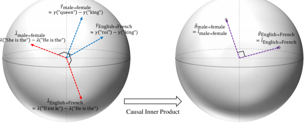
Figure 1: The geometry of linear representations can be understood in terms of a causal inner product that respects the semantic structure of concepts. We show that this inner product induces a unified linear representation of concepts. Generally, each concept has a representation $\bar{\lambda}$ in the embedding (input phrase) space and $\bar{\gamma}$ in the unembedding (output word) space. The left figure shows representations of concepts $W$ and $Z$ induced by a non-causal inner product (e.g., Euclidean). The right figure shows the representation induced by a causal inner product (a linear transformation of the representation space such that the causal inner product becomes Euclidean). In this space, the embedding and unembedding representations are unified, and causally separable concepts are represented by orthogonal vectors.

Next, suppose we have somehow found the linear representations of various concepts. The appeal of linearity is that we can now hope to use linear algebraic operations on the representation space for interpretation and control. For example, we might compute the similarity between a representation and known concept directions, or edit representations projected onto target directions. However, similarity and projection are geometric notions: they require an inner product on the representation space. The second challenge is that it is not clear what inner product is appropriate for understanding model representations.

To address these two challenges, we make the following contributions:

1. First, we formalize the subspace notion of linear representation in terms of counterfactual pairs, in both “embedding” (input phrase) and “unembedding” (output word) space. Using this, we prove that the unembedding notion connects to measurement, and the embedding notion to intervention.

2. Next, we introduce the notion of a causal inner product: an inner product with the property that concepts that can vary freely of each other are represented as orthogonal vectors. We show that such an inner product has the special property that it unifies the embedding and unembedding representations; illustrated in fig. 1. Additionally, we show how to estimate the inner product using the LLM unembedding matrix.

3. Finally, we study the linear representation hypothesis empirically using LLaMA-2 [Tou+23]. Using the subspace notion, we are able to find linear representations of a variety of concepts. Using these, we give evidence that the causal inner product respects semantic structure, and that subspace representations can be used to construct measurement and intervention representations.

Background on Language Models

We will require some minimal background on (large) language models. Formally, a language model takes in context text $x$ and samples output text. This sampling is done word by word (or token by token). Accordingly, we’ll view the outputs as single words. To define a probability distribution over outputs, the language model first maps each context $x$ to a vector $\lambda(x)$ in a representation space $\Lambda\simeq\mathbb{R}^{d}$. We will call these embedding vectors. The model also represents each word $y$ as an unembedding vector $\gamma(y)$ in a separate representation space $\Gamma\simeq\mathbb{R}^{d}$. The probability distribution over the next words is then given by the softmax distribution:

$$\mathbb{P}(y\leavevmode\nobreak\ |\leavevmode\nobreak\ x)\propto\exp(\lambda(x)^{\top}\gamma(y)).$$ (1.1)

2 The Linear Representation Hypothesis

We begin by formalizing the subspace notion of linear representation, one in each of the unembedding and embedding spaces of language models, and then tie the subspace notions to the measurement and intervention notions.

2.1 Concepts

The first step is to formalize the notion of a concept. Intuitively, a concept is any factor of variation that can be changed in isolation. For example, we can change the output from French to English without changing its meaning, or change the output from being about a man to about a woman without changing the language it is written in.

Following [Wan+23], we formalize this idea by taking a concept variable $W$ to be a latent variable that is caused by the context $X$, and that acts as a cause of the output $Y$. For simplicity of exposition, we will restrict attention to binary concepts. Anticipating the representation of concepts by vectors, we introduce an ordering on each binary concept—e.g., male$\Rightarrow$female. This ordering will make the sign of a representation meaningful (so, e.g., the representation of female$\Rightarrow$male will have the opposite sign.)

Each concept variable $W$ defines a set of counterfactual outputs $\{Y(W=w)\}$ that differ only in the value of $W$. For example, for the male$\Rightarrow$female concept, we might have

$$(Y(W=0),Y(W=1))\in_{R}\{(\text{``man''},\text{``woman''}),(\text{``king''},\text{``queen''}),\dots\}$$ (2.1)

In this paper, we’ll assume that the value of concepts can be read off deterministically from the sampled output (so, e.g., the output “king” implies $W=0$). Then, can specify concepts by specifying their corresponding counterfactual outputs.

We will eventually need to reason about the relationships between multiple concepts. We say that two concepts $W$ and $Z$ are causally separable if $Y(W=w,Z=z)$ is well-defined for each $w,z$. That is, causally separable concepts are those that can be varied freely and in isolation. For example, English$\Rightarrow$French and male$\Rightarrow$female are causally separable—consider $\{\text{``king''},\text{``queen''},\text{``roi''},\text{``reine''}\}$. However, English$\Rightarrow$French and English$\Rightarrow$Russian are not because they cannot vary freely. Also, PresentTense$\Rightarrow$PastTense—verb tense—and SingularNoun$\Rightarrow$PluralNoun—noun plurality—are not because they do not apply to the same type of outputs.

We’ll write $Y(W=w,Z=z)$ as $Y(w,z)$ when the concepts are clear from context.

2.2 Unembedding Representations and Measurement

We now turn to formalizing the idea of linear representation of a concept. The first observation is that there are two distinct representation spaces in play—the model representation space $\Lambda$, and the unembedding representation space $\Gamma$. A concept could be linearly represented in either space. We begin with the unembedding space. Defining the cone of vector $v$ as $\operatorname{Cone}(v)=\{\alpha v:\alpha>0\}$,

Definition 1 (Unembedding Representation).

We say that $\bar{\gamma}_{W}$ is an unembedding representation of concept $W$ if $\gamma(Y(1))-\gamma(Y(0))\in\operatorname{Cone}(\bar{\gamma}_{W})$ almost surely.

This definition captures the idea of linear representation that relies on $\gamma(\text{``king''})-\gamma(\text{``queen''})$ is parallel to $\gamma(\text{``man''})-\gamma(\text{``woman''})$ and so forth. We use a cone instead of subspace because the sign of the difference is significant—i.e., the difference between “king” and “queen” is in the opposite direction as the difference between “woman” and “man”. The unembedding representation (if it exists) is unique up to positive scaling, consistent with the linear subspace hypothesis that concepts are represented as directions. In other words, the unembedding representation is the unique direction that the counterfactual pairs point to in the unembedding space.

Connection to Measurement

The first result is that the unembedding representation is closely tied to the measurement notion of linear representation:

Theorem 2 (Measurement Representation).

Let $W$ be a concept, and let $\bar{\gamma}_{W}$ be an unembedding representation of $W$. Then, given any context embedding $\lambda\in\Lambda$,

$$\operatorname*{logit}\mathbb{P}(Y=Y(1)\leavevmode\nobreak\ |\leavevmode\nobreak\ Y\in\{Y(1),Y(0)\},\lambda)=\alpha\lambda^{\top}\bar{\gamma}_{W},$$ (2.2)

where $\alpha>0$ a.s. is a function of $\{Y(1),Y(0)\}$.

All proofs are given in Appendix A.

In words: if we know the output token is either “king” or “queen” (say, the context was about a monarch), then the probability that the output is “king” is logit-linear in the language model representation with regression coefficients $\bar{\gamma}_{W}$. The random scalar $\alpha$ is a function of the particular counterfactual pair $\{Y(1),Y(0)\}$—e.g., it may be different for $\{\text{``king''},\text{``queen''}\}$ and $\{\text{``roi''},\text{``riene''}\}$. However, the direction used for prediction is the same for all counterfactual pairs demonstrating the concept.

Theorem 2 shows a connection between the subspace representation and the linear representation learned by fitting a linear probe to predict the concept. Namely, in both cases, we get a predictor that is linear on the logit scale. However, the unembedding representation differs from a probe-based representation in that it does not incorporate any information about correlated but off-target concepts. For example, if French text were disproportionately about men, a probe could learn this information (and include it in the representation), but the unembedding representation would not. In this sense, the unembedding representation might be viewed as an ideal probing representation.

2.3 Embedding Representations and Intervention

The next step is to define a linear subspace representation in the embedding space $\Lambda$. We’ll again go with a notion anchored in demonstrative pairs. In the embedding space, each $\lambda(x)$ defines a distribution over concepts. We consider pairs of sentences such as $\lambda_{0}=\lambda[\text{``He is the monarch of England,''}]$ and $\lambda_{1}=\lambda[\text{``She is the monarch of England,''}]$ that induce different distributions on the target concept, but the same distribution on all off-target concepts. A concept is embedding-represented if the difference in all such pairs belongs to a common subspace. Formally,

Definition 3 (Embedding Representation).

We say that $\bar{\lambda}_{W}$ is an embedding representation of concept $W$ if for any context embeddings $\lambda_{0},\lambda_{1}\in\Lambda$ that satisfy

$$\frac{\mathbb{P}(W=1\leavevmode\nobreak\ |\leavevmode\nobreak\ \lambda_{1})}{\mathbb{P}(W=1\leavevmode\nobreak\ |\leavevmode\nobreak\ \lambda_{0})}>1\quad\text{and}\quad\frac{\mathbb{P}(W,Z\leavevmode\nobreak\ |\leavevmode\nobreak\ \lambda_{1})}{\mathbb{P}(W,Z\leavevmode\nobreak\ |\leavevmode\nobreak\ \lambda_{0})}=\frac{\mathbb{P}(W\leavevmode\nobreak\ |\leavevmode\nobreak\ \lambda_{1})}{\mathbb{P}(W\leavevmode\nobreak\ |\leavevmode\nobreak\ \lambda_{0})},$$ (2.3)

for each concept $Z$ that is causally separable with $W$, we have $\lambda_{1}-\lambda_{0}\in\operatorname{Cone}(\bar{\lambda}_{W})$.

The first condition ensures that the direction is relevant to the target concept, and the second condition ensures that the direction is not relevant to off-target concepts.

Connection to Intervention

It turns out that the embedding representation is closely tied to the intervention notion of linear representation. To get there, we’ll need the following lemma relating embedding representations to unembedding representations.

Lemma 4 (Unembedding-Embedding Relationship).

Let $\bar{\lambda}_{W}$ be the embedding representation of a concept $W$, and let $\bar{\gamma}_{W}$ and $\bar{\gamma}_{Z}$ be the unembedding representations for $W$ and any concept $Z$ that is causally separable with $W$. Then, we have

$$\bar{\lambda}_{W}^{\top}\bar{\gamma}_{W}>0\quad\text{and}\quad\bar{\lambda}_{W}^{\top}\bar{\gamma}_{Z}=0.$$ (2.4)

Conversely, if a representation $\bar{\lambda}_{W}$ satisfies (2.4) and there exist concepts $\{Z_{i}\}_{i=1}^{d-1}$ such that each concept is causally separable with $W$ and $\{\bar{\gamma}_{W}\}\cup\{\bar{\gamma}_{Z_{i}}\}_{i=1}^{d-1}$ is the basis of $\mathbb{R}^{d}$, then $\bar{\lambda}_{W}$ is the embedding representation for the concept $W$.

We can now give the connection to the intervention notion of linear representation.

Theorem 5 (Intervention Representation).

Let $\bar{\lambda}_{W}$ be the embedding representation of a concept $W$. Then, for any concept $Z$ that is causally separable with $W$,

$$\mathbb{P}(Y=Y(W,1)\leavevmode\nobreak\ |\leavevmode\nobreak\ Y\in\{Y(W,0),Y(W,1)\},\lambda+c\bar{\lambda}_{W})\text{ is constant in }c\in\mathbb{R},$$ (2.5)

and

$$\mathbb{P}(Y=Y(1,Z)\leavevmode\nobreak\ |\leavevmode\nobreak\ Y\in\{Y(0,Z),Y(1,Z)\},\lambda+c\bar{\lambda}_{W})\text{ is increasing in }c\in\mathbb{R}.$$ (2.6)

In words: adding $\bar{\lambda}_{W}$ to the language model representation of the context changes the probability of the target concept, but not the probability of off-target concepts.

3 Inner Product for Language Model Representations

Given linear representations, we would like to make use of them by doing things like measuring the similarity between different representations, or editing concepts by projecting onto a target direction. Similarity and projection are both notions that require an inner product. We now consider the question of which inner product is appropriate for understanding language model representations.

Preliminaries

We define $\bar{\Gamma}$ to be the space of differences between elements of $\Gamma$. Then, $\bar{\Gamma}$ is a $d$-dimensional real vector space. We consider defining inner products on $\bar{\Gamma}$. Unembedding representations are naturally directions (unique only up to scale). Once we have an inner product, we define the canonical unembedding representation $\bar{\gamma}_{W}$ to be the element of the unembedding cone with $\langle\bar{\gamma}_{W},\bar{\gamma}_{W}\rangle=1$. This lets us define inner products between unembedding representations.

Unidentifiability of the inner product

We might hope that there is some natural inner product that is picked out (identified) by the model training. It turns out that this is not the case. To understand the challenge, consider transforming the embedding and unembedding spaces according to

$$g(y)\leftarrow A\gamma(y)+\beta,\quad l(x)\leftarrow A^{-\top}\lambda(x),$$ (3.1)

where $A\in\mathbb{R}^{d\times d}$ is some invertible linear transformation and $\beta\in\mathbb{R}^{d}$ is a constant. It’s easy to see that this transformation preserves the softmax distribution $\mathbb{P}(y\leavevmode\nobreak\ |\leavevmode\nobreak\ x)$:

$$\frac{\exp(\lambda(x)^{\top}\gamma(y))}{\sum_{y^{\prime}}\exp(\lambda(x)^{\top}\gamma(y^{\prime}))}=\frac{\exp(l(x)^{\top}g(y))}{\sum_{y^{\prime}}\exp(l(x)^{\top}g(y^{\prime}))}\quad\forall x,y.$$ (3.2)

However, the objective function used to train the model depends on the representations only through the softmax probabilities. Thus, the representation $\gamma$ is identified (at best) only up to some invertible affine transformation.

This also means that the concept representations $\bar{\gamma}_{W}$ are identified only up to some invertible linear transformation $A$. The problem is that, given any fixed inner product,

$$\langle\bar{\gamma}_{W},\bar{\gamma}_{Z}\rangle\neq\langle A\bar{\gamma}_{W},A\bar{\gamma}_{Z}\rangle,$$ (3.3)

in general. Accordingly, there is no obvious reason to expect that algebraic manipulations based on, e.g., the Euclidean inner product, should be preferred to manipulations using any other inner product.

3.1 Causal Inner Products

We require some additional principles for choosing an inner product on the representation space. The intuition we follow here is that causally separable concepts should be represented as orthogonal vectors. For example, French$\Rightarrow$English and Male$\Rightarrow$Female, should be orthogonal. We define an inner product with this property:

Definition 6 (Causal Inner Product).

A causal inner product $\langle\cdot,\cdot\rangle_{\mathrm{C}}$ on $\bar{\Gamma}\simeq\mathbb{R}^{d}$ is an inner product such that

$$\langle\bar{\gamma}_{W},\bar{\gamma}_{Z}\rangle_{\mathrm{C}}=0,$$ (3.4)

for any pair of causally separable concepts $W$ and $Z$.

This choice turns out to have the critical property that it gives a natural unification of the unembedding and embedding representations:

Theorem 7 (Unification of Representations).

Suppose that, for any concept $W$, there exist concepts $\{Z_{i}\}_{i=1}^{d-1}$ such that each concept is causally separable with $W$ and $\{\bar{\gamma}_{W}\}\cup\{\bar{\gamma}_{Z_{i}}\}_{i=1}^{d-1}$ is a basis of $\mathbb{R}^{d}$. If $\langle\cdot,\cdot\rangle_{\mathrm{C}}$ is a causal inner product, then the Riesz isomorphism $\bar{\gamma}\mapsto\langle\bar{\gamma},\cdot\rangle_{\mathrm{C}}$ maps the unembedding representation $\bar{\gamma}_{W}$ of each concept $W$ to its embedding representation $\bar{\lambda}_{W}$:

$$\langle\bar{\gamma}_{W},\cdot\rangle_{\mathrm{C}}=\bar{\lambda}_{W}^{\top}.$$ (3.5)

To understand this result intuitively, notice we can represent embeddings as row vectors and unembeddings as column vectors. If the causal inner product was the Euclidean inner product, the isomorphism would simply be the transpose operation. The theorem is the (Riesz isomorphism) generalization of this idea: Each linear map on $\bar{\Gamma}$ corresponds to some $\lambda\in\Lambda$ according to $\lambda^{\top}:\bar{\gamma}\mapsto\lambda^{\top}\bar{\gamma}$. So, we can map $\Gamma$ to $\Lambda$ by mapping each $\bar{\gamma}_{W}$ to a linear function according to $\bar{\gamma}_{W}\to\langle\bar{\gamma}_{W},\cdot\rangle_{\mathrm{C}}$. The theorem says this map sends each unembedding representation of a concept to the embedding representation of the same concept.

In the experiments, we will make use of this result to construct embedding representations from unembedding representations. In particular, this allows us to find interventional representations of concepts. This is important because it is difficult in practice to find pairs of prompts that directly satisfy Definition 3.

3.2 An Explicit Form for Causal Inner Product

The next problem is: if a causal inner product exists, how can we find it? In principle, this could be done by finding the unembedding representations of a large number of concepts, and then finding an inner product that maps each pair of causally separable directions to zero. In practice, this is infeasible because of the number of concepts required to find the inner product, and the difficulty of estimating the representations of each concept.

We now turn to developing a more tractable approach. Our technique is based on the following insight: knowing the value of concept $W$ expressed by a randomly chosen word tells us little about the value of that word on a causally separable concept $Z$. For example, if we learn that a randomly sampled word is French (not English), this does not give us significant information about whether it refers to a man or woman. Following Theorem 5, we formalize this idea as follows:

Assumption 1.

Suppose $W,Z$ are causally separable concepts and that $\gamma$ is an unembedding vector sampled uniformly from the vocabulary. Then, $\bar{\lambda}_{W}^{\top}\gamma\mathchoice{\mathrel{\hbox to0.0pt{$\displaystyle\perp$\hss}\mkern 2.0mu{\displaystyle\perp}}}{\mathrel{\hbox to0.0pt{$\textstyle\perp$\hss}\mkern 2.0mu{\textstyle\perp}}}{\mathrel{\hbox to0.0pt{$\scriptstyle\perp$\hss}\mkern 2.0mu{\scriptstyle\perp}}}{\mathrel{\hbox to0.0pt{$\scriptscriptstyle\perp$\hss}\mkern 2.0mu{\scriptscriptstyle\perp}}}\bar{\lambda}_{Z}^{\top}\gamma$ for any embedding representations $\bar{\lambda}_{W}$ and $\bar{\lambda}_{Z}$ for $W$ and $Z$, respectively.

This assumption lets us connect causal separability with something we can actually measure: the statistical dependency between words. The next result makes this precise.

Theorem 8 (Explicit Form of Causal Inner Product).

Suppose a causal inner product, represented as $\langle\bar{\gamma},\bar{\gamma}^{\prime}\rangle_{\mathrm{C}}=\bar{\gamma}^{\top}M\bar{\gamma}^{\prime}$ for some symmetric positive definite matrix $M$, exists. If there are mutually causally separable concepts $\{W_{k}\}_{k=1}^{d}$, such that their canonical representations $G=[\bar{\gamma}_{W_{1}},\cdots,\bar{\gamma}_{W_{d}}]$ form a basis for $\bar{\Gamma}\simeq\mathbb{R}^{d}$, then under Assumption 1,

$$M^{-1}=GG^{\top}\text{ and }G^{\top}\mathrm{Cov}(\gamma)^{-1}G=D,$$ (3.6)

for some diagonal matrix $D$ with positive entries, where $\gamma$ is the unembedding vector of a word sampled uniformly at random from the vocabulary.

Notice that causal orthogonality only imposes $d(d-1)/2$ constraints on the inner product, but there are $d(d-1)/2+d$ degrees of freedom in defining a positive definite matrix (hence, an inner product)—thus, we expect $d$ degrees of freedom in choosing a causal inner product. Theorem 8 gives a characterization of this class of inner products, in the form of (3.6). Here, $D$ is a free parameter with $d$ degrees of freedom. Each $D$ defines the inner product. We do not have a principle for picking out a unique choice of $D$ (and thus, a unique inner product). In our experiments, we will work with the choice $D=I_{d}$. Then, we have a simple closed form for the corresponding inner product:

$$\langle\bar{\gamma},\bar{\gamma}^{\prime}\rangle_{\mathrm{C}}:=\bar{\gamma}^{\top}\mathrm{Cov}(\gamma)^{-1}\bar{\gamma}^{\prime},\quad\forall\bar{\gamma},\bar{\gamma}^{\prime}\in\bar{\Gamma}.$$ (3.7)

Notice that although we don’t have a unique inner product, we can rule out most inner products. E.g., the Euclidean inner product is not a causal inner product if $M=I_{d}$ does not satisfy (3.6) for any $D$.

Canonical representation

The choice of inner product also be viewed as defining a canonical choice of representations $g,l$ in eq. 3.1. Namely, we define

$$g(y)=\mathrm{Cov}(\gamma)^{-1/2}\gamma(y)\quad\text{and}\quad l(x)=\mathrm{Cov}(\gamma)^{1/2}\lambda(x),$$ (3.8)

for some square root of the inverse covariance matrix. It is easy to see that this choice makes the embedding and unembedding representations of concepts the same, $\bar{g}_{W}=\bar{l}_{W}$, and that $\langle\bar{\gamma},\bar{\gamma}^{\prime}\rangle_{\mathrm{C}}=\bar{g}^{\top}\bar{g}^{\prime}$. That is, $g$ is a representation where the Euclidean inner product is a causal inner product. So, we can view a choice of inner product as instead being a choice of representation. This is illustrated in fig. 1. This is convenient for experiments, because it allows the use of standard Euclidean tools on the transformed space.

4 Experiments

We now turn to empirically validating the existence of linear representations, the technique for finding the causal inner product, and the predicted relationships between the subspace, measurement, and intervention notions of linear representation. Code available at github.com/KihoPark/linear_rep_geometry.

We use the LLaMA-2 model with 7 billion parameters [Tou+23] as our testbed. This is a decoder-only Transformer LLM [Vas+17, Rad+18], trained using the forward LM objective and a 32K token vocabulary.

4.1 Concepts are represented as directions in the unembedding space

We start with the hypothesis that concepts are represented as directions in the unembedding representation space (Definition 1). This notion relies on counterfactual pairs of words that vary only in the value of the concept of interest. We consider 22 concepts defined in the Big Analogy Test Set (BATS 3.0) [GDM16], which provides such counterfactual pairs. We also consider 4 additional language concepts: English$\Rightarrow$French, French$\Rightarrow$German, French$\Rightarrow$Spanish, and German$\Rightarrow$Spanish, where we use words and their translations as counterfactual pairs. Additionally, we consider the concept frequent$\Rightarrow$infrequent capturing how common a word is—we use pairs of common/uncommon synonyms (e.g., “bad” and “terrible”) as counterfactual pairs. In Appendix B, we list all 27 concepts we consider and example pairs.

If the subspace notion of the linear representation hypothesis holds then all counterfactual token pairs should point to a common direction in the unembedding space. In practice, this will only hold approximately for real pairs because each word can have multiple meanings (e.g., “Queen” is a female monarch, a chess piece, and a rock band). However, if the linear representation hypothesis holds, we still expect that $\gamma(\text{``King''})-\gamma(\text{``Queen''})$ will significantly align with a male$\Rightarrow$female direction. So, for each concept $W$, we look at how the direction defined by each counterfactual pair $\gamma(y_{i}(1))-\gamma(y_{i}(0))$ is geometrically aligned with a common direction $\bar{\gamma}_{W}$ (the unembedding representation). We estimate $\bar{\gamma}_{W}$ as the mean among all counterfactual pairs:

$$\bar{\gamma}_{W}:=\frac{\tilde{\gamma}_{W}}{\sqrt{\langle\tilde{\gamma}_{W},\tilde{\gamma}_{W}\rangle_{\mathrm{C}}}},\quad\text{with}\quad\tilde{\gamma}_{W}=\frac{1}{n_{W}}\sum_{i=1}^{n_{W}}\gamma(y_{i}(1))-\gamma(y_{i}(0)),$$ (4.1)

where $\langle\cdot,\cdot\rangle_{\mathrm{C}}$ denotes the causal inner product defined in (3.7).

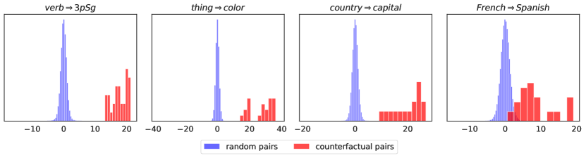
Figure 2: Projecting counterfactual pairs onto their corresponding concept direction shows a clear strong right skew, as we expect if the linear representation hypothesis holds. The projections of the counterfactual pairs, $\langle\bar{\gamma}_{W,(-i)},\gamma(y_{i}(1))-\gamma(y_{i}(0))\rangle_{\mathrm{C}}$, are shown in red. For reference, we also project 100K randomly sampled word differences $\gamma(Y_{i_{1}})-\gamma(Y_{i_{0}})$ onto the estimated concept direction, shown in blue. Each concept $W$ (the title of each plot) is explained in Table 2.

Figure 2 presents histograms of each $\gamma(y_{i}(1))-\gamma(y_{i}(0)))$ projected onto $\bar{\gamma}_{W}$ with respect to the causal inner product. Because $\bar{\gamma}_{W}$ is computed using $\gamma(y_{i}(1))-\gamma(y_{i}(0))$, we compute each projection using a leave-one-out (LOO) estimate $\bar{\gamma}_{W,(-i)}$ of the concept direction that excludes $(y_{i}(0),y_{i}(1))$. Across the four concepts shown (and 22 others shown in Appendix C), the differences between counterfactual pairs are substantially more aligned with $\bar{\gamma}_{W}$ than those between random pairs. The sole exception is thing$\Rightarrow$part, which does not appear to have a linear representation.

The results are consistent with the linear representation hypothesis: the directions computed by each counterfactual pair point (up to some noise) to a common direction representing a linear subspace. Further, $\bar{\gamma}_{W}$ is a reasonable estimator for that direction.

4.2 Concept directions act as linear probes

Next, we check the connection to the measurement notion of linear representation. We consider the concept French$\Rightarrow$Spanish. To construct a dataset of French/Spanish contexts, we sample contexts of random lengths from Wikipedia pages in each language. (Note: these are not counterfactual pairs.) Following Theorem 2 we expect $\bar{\gamma}_{W}^{\top}\lambda(x_{j}^{\texttt{fr}})<0$ and $\bar{\gamma}_{W}^{\top}\lambda(x_{j}^{\texttt{es}})>0$. Figure 3 confirms this expectation, showing that $\bar{\gamma}_{W}$ is a linear probe for the concept $W$ in $\Lambda$. We also see that the representation of an off-target concept $Z$ does not have any predictive power for this task.

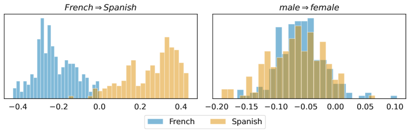
Figure 3: The subspace representation $\bar{\gamma}_{W}$ acts as a linear probe for $W$. The histograms show $\bar{\gamma}_{W}^{\top}\lambda(x_{j}^{\texttt{fr}})$ vs. $\bar{\gamma}_{W}^{\top}\lambda(x_{j}^{\texttt{es}})$ (left) and $\bar{\gamma}_{Z}^{\top}\lambda(x_{j}^{\texttt{fr}})$ vs. $\bar{\gamma}_{Z}^{\top}\lambda(x_{j}^{\texttt{es}})$ (right) for $W=$ French$\Rightarrow$Spanish and $Z=$ male$\Rightarrow$female, where $\{x_{j}^{\texttt{fr}}\}$ are random contexts from French Wikipedia, and $\{x_{j}^{\texttt{es}}\}$ are random contexts from Spanish Wikipedia. We also see that $\bar{\gamma}_{Z}$ does not act as a linear probe for $W$, as expected.

4.3 Concept directions map to intervention representations

Theorem 5 says that we can construct an intervention representation by constructing an embedding embedding representation. Doing this directly requires finding pairs of prompt that vary only on the distribution they induce on the target concept. In preliminary experiments, we found it was difficult to construct such pairs in practice.

Here, we will instead use the isomorphism between embedding and unembedding representations (Theorem 7) to construct intervention representations from unembedding representations. We take

$$\bar{\lambda}_{W}:=\mathrm{Cov}(\gamma)^{-1}\bar{\gamma}_{W}.$$ (4.2)

Theorem 5 predicts that adding $\bar{\lambda}_{W}$ to a context representation should increase the probability of $W$, while leaving the probability of all causally separable concepts unaltered.

To test this for a given pair of causally separable concepts $W$ and $Z$, we first choose a quadruple $\{Y(w,z)\}_{w,z\in\{0,1\}}$, and then generate contexts $\{x_{j}\}$ such that the next word should be $Y(0,0)$. For example, if $W=$ male$\Rightarrow$female and $Z=$ lower$\Rightarrow$upper, then we choose the quadruple (“king”, “queen”, “King”, “Queen”), and generate contexts using ChatGPT-4 (e.g., “Long live the”). We then intervene on $\lambda(x_{j})$ using $\bar{\lambda}_{C}$ via

$$\lambda_{C,\alpha}(x_{j})=\lambda(x_{j})+\alpha\bar{\lambda}_{C},$$ (4.3)

where $\alpha>0$ and $C$ can be $W$, $Z$, or some other causally separable concept (e.g., French$\Rightarrow$Spanish). For different choices of $C$, we plot the changes in $\operatorname*{logit}\mathbb{P}(W=1\leavevmode\nobreak\ |\leavevmode\nobreak\ Z,\lambda)$ and $\operatorname*{logit}\mathbb{P}(Z=1\leavevmode\nobreak\ |\leavevmode\nobreak\ W,\lambda)$, as we increase $\alpha$. We expect to see that, if we intervene in the $W$ direction ($C=W$), then the intervention should linearly increase $\operatorname*{logit}\mathbb{P}(W=1\leavevmode\nobreak\ |\leavevmode\nobreak\ Z,\lambda)$, while the other logit should stay constant; if we intervene in a direction $C$ that is causally separable with both $W$ and $Z$, then we expect both logits to stay constant.

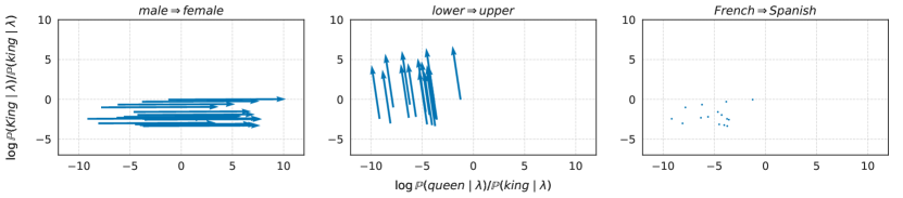
Figure 4: Adding $\alpha\bar{\lambda}_{C}$ to $\lambda$ changes the target concept $C$ without changing off-target concepts. The plots illustrate change in $\log(\mathbb{P}(\mathrm{``queen"}\leavevmode\nobreak\ |\leavevmode\nobreak\ x)/\mathbb{P}(\mathrm{``king"}\leavevmode\nobreak\ |\leavevmode\nobreak\ x))$ and $\log(\mathbb{P}(\mathrm{``King"}\leavevmode\nobreak\ |\leavevmode\nobreak\ x)/\mathbb{P}(\mathrm{``king"}\leavevmode\nobreak\ |\leavevmode\nobreak\ x))$, after changing $\lambda(x_{j})$ to $\lambda_{C,\alpha}(x_{j})$ ($\alpha\in[0,0.4]$) and $C=$ male$\Rightarrow$female (left), lower$\Rightarrow$upper (center), French$\Rightarrow$Spanish (right). The two ends of the arrow are $\lambda(x_{j})$ and $\lambda_{C,0.4}(x_{j})$, respectively. Each context $x_{j}$ is presented in Table 4.

Figure 4 shows the results of one such experiment, confirming our expectations. We see, for example, that intervening in the male$\Rightarrow$female direction raises the logit for choosing “queen” over “king” as the next word, but does not change the logit for “King” over “king”.

(a) Context: “Long live the ”

Rank	$\alpha=$ 0	0.1	0.2	0.3	0.4
1	king	Queen	queen	queen	queen
2	King	queen	Queen	Queen	Queen
3	Queen	king	_	lady	lady
4	queen	King	lady	woman	woman
5	_	_	king	women	women

(b) Context: “In a monarchy, the ruler is usually a ”

Rank	$\alpha=$ 0	0.1	0.2	0.3	0.4
1	king	king	her	woman	woman
2	monarch	monarch	monarch	queen	queen
3	member	her	member	her	female
4	her	member	woman	monarch	her
5	person	person	queen	member	member

Table 1: Adding the intervention representation $\alpha\bar{\lambda}_{W}$ changes the probability over completions in the expected way. As the scale of intervention increases, the probability of seeing $Y(W=1)$ (“queen”) increases while the probability of seeing $Y(W=0)$ (“king”) decreases. We show the top-5 most probable words after the intervention (4.3) in the $W=$ male$\Rightarrow$female direction, i.e., $\lambda_{W,\alpha}(x)=\lambda(x)+\alpha\bar{\lambda}_{W}$, for $\alpha\in\{0,0.1,0.2,0.3,0.4\}$. The original context $x$ is a sentence fragment that ends with the word $Y(W=0)$ (“king”). The most likely words reflect the concept, with “queen” being (close to) top-1.

A natural follow-up question is to see if, e.g., the intervention in the male$\Rightarrow$female direction pushes the probability of “queen” being the next word to the largest among all tokens. We expect to see that, as we increase the value of $\alpha$, the target concept (female) should eventually be reflected in the most likely output words according to the LM. In Table 1, we show two illustrative examples in which $W$ is the concept male$\Rightarrow$female and the context $x$ is a sentence fragment that can end with the word $Y(W=0)$ (“king”). In the first example ($x=$ “Long live the ”), as we increase the scale $\alpha$ on the intervention, we see that the target word $Y(W=1)$ (“queen”) becomes the most likely next word, while the original word $Y(W=0)$ drops below the top-5 list. This illustrates how the intervention can push the probability of the target word high enough to make it the most likely word while decreasing the probability of the original word. The second example ($x=$ “In a monarchy, the ruler usually is a ”) further shows that, even when the target word does not become the most likely one, the most likely words reflect the concept direction (“woman”, “queen”, “her”, “female”).

4.4 The estimated inner product respects causal separability

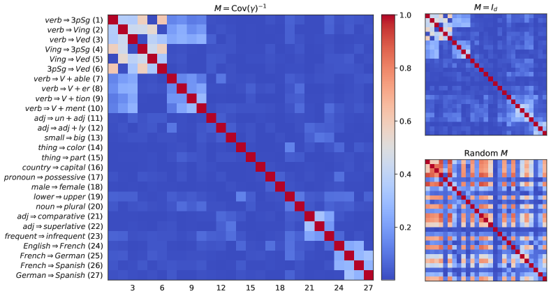
Figure 5: Causally separable concepts are approximately orthogonal under the estimated causal inner product. The heatmaps show $|\langle\bar{\gamma}_{W},\bar{\gamma}_{Z}\rangle|$ for the estimated unembedding representations of each concept pair $(W,Z)$. The plot on the left shows the estimated inner product based on (3.7). We also consider two reference inner products by varying the choice of the symmetric positive definite matrix $M$. The upper-right plot represents Euclidean inner product ($M=I_{d}$); the lower-right plot represents an arbitrary inner product ($M=A^{\top}A$, where $A_{i,j}=\left\lvert a_{i,j}\right\rvert$ and $a_{i,j}\overset{\mathrm{iid}}{\ \sim\ }N(0,1)$). The detail for the concepts is given in Table 2. See main text for a discussion of the interpretation.

Finally, we turn to directly examining whether the estimated inner product chosen from Theorem 8,

$$\langle\bar{\gamma},\bar{\gamma}^{\prime}\rangle_{\mathrm{C}}:=\bar{\gamma}^{\top}\mathrm{Cov}(\gamma)^{-1}\bar{\gamma}^{\prime},\quad\forall\bar{\gamma},\bar{\gamma}^{\prime}\in\bar{\Gamma},$$ (4.4)

is indeed approximately a causal inner product. In fig. 5, we plot a heatmap of the inner products between all pairs of the 27 estimated concepts. If the estimated inner product is a causal inner product, then we expect values near 0 between causally separable concepts (and large values between causally related concepts).

The first observation is that most pairs of concepts are nearly orthogonal with respect to this inner product. Interestingly, there is also a clear block diagonal structure. This arises because the concepts are grouped by semantic similarity. For example, the first 10 concepts relate to verbs, and the last 4 concepts are language pairs. The additional non-zero structure also generally makes sense. For example, lower$\Rightarrow$upper (capitalization, concept 19) has non-trivial inner product with the language pairs other than French$\Rightarrow$Spanish. This may be because French and Spanish obey similar capitalization rules, while English and German each have different conventions (e.g., German capitalizes all nouns, but English only capitalizes proper nouns).

In fig. 5, we also plot the similarities induced by the Euclidean inner product ($M=I_{d}$) and an arbitrarily chosen inner product ($M=A^{\top}A$, where $A_{i,j}=\left\lvert a_{i,j}\right\rvert$ and $a_{i,j}\overset{\mathrm{iid}}{\ \sim\ }N(0,1)$). We see that the arbitrary inner product does not respect the semantic structure at all. Surprisingly, the Euclidean inner product somewhat does! This may due to some initialization or implicit regularizing effect that favors learning unembeddings with approximately isotropic covariance. Nevertheless, the estimated causal inner product clearly improves on the Euclidean inner product. For example, frequent$\Rightarrow$infrequent (concept 23) has high Euclidean inner product with many separable concepts, and these are much smaller for the causal inner product. Conversely, English$\Rightarrow$French (24) has low Euclidean inner product with the other language concepts (25-27), but high causal inner product with French$\Rightarrow$German and French$\Rightarrow$Spanish (while being nearly orthogonal to German$\Rightarrow$Spanish, which does not share French.).

5 Discussion and Related Work

The idea that high-level concepts are encoded linearly is appealing because—if it is true—it may open up simple methods for interpretability and controllability of LLMs. In this paper, we have formalized ‘linear representation’, and shown that all natural variants of this notion can be unified. This equivalence already suggests some approaches for interpretation and control—e.g., we show how to use collections of pairs of words to define concept directions (Section 4.1), and then use these directions to predict what the model’s output will be (Section 4.2), and to change the output in a controlled fashion (Section 4.3). A major theme is the role played by the choice of inner product.

Linear subspaces in language representations

The linear subspace hypotheses was originally observed empirically in the context of word embeddings [Mik+13, LG14, GL14, Vyl+16, GDM16, CCCP20, FDD20, e.g.,]. Similar structure has been observed in cross-lingual word embeddings [MLS13, Lam+18, RVS19, Pen+22], sentence embeddings [Bow+16, ZM20, Li+20, Ush+21], representation spaces of Transformer LLMs [Men+22, MEP23, Her+23], and vision-language models [Wan+23, Tra+23, Per+23]. These observations motivate Definition 1. The key idea in the present paper is providing formalization in terms of counterfactual pairs—this is what allows us to connect to other notions of linear representation, and to identify the inner product structure.

Measurement, intervention, and mechanistic interpretability

There is a significant body of work on linear representations for interpreting (probing) [AB17, Kim+18, nos20, RKR21, Bel22, Li+22, Gev+22, NLW23, e.g.,] and controlling (steering) [Wan+23, Tur+23, MEP23, Tra+23, e.g.,] models. This is particularly prominent in mechanistic interpretability [Elh+21, Men+22, Her+23, Tur+23, Zou+23, Tod+23, HGG23]. With respect to this body of work, the main contribution of the present paper is to clarify the linear representation hypothesis, and the critical role of the inner product. However, we do not address interpretability of either model parameters, nor the activations of intermediate layers. These are main focuses of existing work. It is an exciting direction for future work to understand how ideas here—particularly, the causal inner product—translate to these settings.

Geometry of representations

There is a line of work that studies the geometry of word and sentence representations [Aro+16, MT17, Eth19, Rei+19, Li+20, HM19, Che+21, CTB22, JAV23, e.g.,]. This work considers, e.g., visualizing and modeling how the learned embeddings are distributed, or how hierarchical structure is encoded. Our work is largely orthogonal to these, since we are attempting to define a suitable inner product (and thus, notion of distance) that respects the semantic structure of language.

Causal representation learning

Finally, the ideas here connect to causal representation learning [Hig+16, HM16, Hig+18, Khe+20, Zim+21, Sch+21, Mor+21, Wan+23, e.g.,]. Most obviously, our causal formalization of concepts is inspired by [Wan+23], who establish a characterization of latent concepts and vector algebra in diffusion models. Separately, a major theme in this literature is the identifiability of learned representations—i.e., to what extent they capture underlying real-world structure. Our causal inner product results may be viewed in this theme, showing that an inner product respecting semantic closeness is not identified by the usual training procedure, but that it can be picked out with a suitable assumption.

Appendix A Proofs

A.1 Proof of Theorem 2

See 2

Proof.

The proof involves writing out the softmax sampling distribution and invoking Definition 1.

$$\operatorname*{logit}\mathbb{P}(Y=Y(1)\leavevmode\nobreak\ |\leavevmode\nobreak\ Y\in\{Y(1),Y(0)\},\lambda)$$ (A.1)

$$=\log\frac{\mathbb{P}(Y=Y(1)\leavevmode\nobreak\ |\leavevmode\nobreak\ Y\in\{Y(1),Y(0)\},\lambda)}{\mathbb{P}(Y=Y(0)\leavevmode\nobreak\ |\leavevmode\nobreak\ Y\in\{Y(1),Y(0)\},\lambda)}$$ (A.2)

$$=\lambda^{\top}\left\{\gamma(Y(1))-\gamma(Y(0))\right\}$$ (A.3)

$$=\alpha\cdot\lambda^{\top}\bar{\gamma}_{W}.$$ (A.4)

In (A.3), we simply write out the softmax distribution, allowing us to cancel out the normalizing constants for the two probabilities. Equation (A.4) follows directly from Definition 1; note that the randomness of $\alpha$ comes from the randomness of $(Y(1),Y(0))$. ∎

A.2 Proof of Lemma 4

See 4

Proof.

Let $\lambda_{0},\lambda_{1}$ be a pair of embeddings such that

$$\frac{\mathbb{P}(W=1\leavevmode\nobreak\ |\leavevmode\nobreak\ \lambda_{1})}{\mathbb{P}(W=1\leavevmode\nobreak\ |\leavevmode\nobreak\ \lambda_{0})}>1\quad\text{and}\quad\frac{\mathbb{P}(W,Z\leavevmode\nobreak\ |\leavevmode\nobreak\ \lambda_{1})}{\mathbb{P}(W,Z\leavevmode\nobreak\ |\leavevmode\nobreak\ \lambda_{0})}=\frac{\mathbb{P}(W\leavevmode\nobreak\ |\leavevmode\nobreak\ \lambda_{1})}{\mathbb{P}(W\leavevmode\nobreak\ |\leavevmode\nobreak\ \lambda_{0})},$$ (A.5)

for any concept $Z$ that is causally separable with $W$. Then, by Definition 3,

$$\lambda_{1}-\lambda_{0}\in\operatorname{Cone}(\bar{\lambda}_{W}).$$ (A.6)

The condition (A.5) is equivalent to

$$\frac{\mathbb{P}(W=1\leavevmode\nobreak\ |\leavevmode\nobreak\ \lambda_{1})}{\mathbb{P}(W=1\leavevmode\nobreak\ |\leavevmode\nobreak\ \lambda_{0})}>1\quad\text{and}\quad\frac{\mathbb{P}(Z=1\leavevmode\nobreak\ |\leavevmode\nobreak\ W,\lambda_{1})}{\mathbb{P}(Z=1\leavevmode\nobreak\ |\leavevmode\nobreak\ W,\lambda_{0})}=1.$$ (A.7)

These two conditions are also equivalent to the following pair of conditions, respectively:

$$\frac{\mathbb{P}(Y=Y(1)\leavevmode\nobreak\ |\leavevmode\nobreak\ Y\in\{Y(1),Y(0)\},\lambda_{1})}{\mathbb{P}(Y=Y(1)\leavevmode\nobreak\ |\leavevmode\nobreak\ Y\in\{Y(1),Y(0)\},\lambda_{0})}>1$$ (A.8)

and

$$\frac{\mathbb{P}(Y=Y(W,1)\leavevmode\nobreak\ |\leavevmode\nobreak\ Y\in\{Y(W,0),Y(W,1)\},\lambda_{1})}{\mathbb{P}(Y=Y(W,1)\leavevmode\nobreak\ |\leavevmode\nobreak\ Y\in\{Y(W,0),Y(W,1)\},\lambda_{0})}=1$$ (A.9)

The reason is that, conditional on $Y\in\{Y(0,0),Y(0,1),Y(1,0),Y(1,1)\}$, conditioning on $W$ is equivalent to conditioning on $Y\in\{Y(W,0),Y(W,1)\}$. And, the event $Z=1$ is equivalent to the event $Y=Y(W,1)$. (In words: if we know the output is one of “king”, “queen”, “roi”, “reine” then conditioning on $W=1$ is equivalent to conditioning on the output being “king” or “roi”. Then, predicting whether the word is in English is equivalent to predicting whether the word is “king”.)

By Theorem 2, the two conditions (A.8) and (A.9) are respectively equivalent to

$$\alpha(Y(0),Y(1))(\lambda_{1}-\lambda_{0})^{\top}\bar{\gamma}_{W}>0\quad\text{and}\quad\alpha(Y(W,0),Y(W,1))(\lambda_{1}-\lambda_{0})^{\top}\bar{\gamma}_{Z}=0,$$ (A.10)

where $\alpha$’s are positive a.s. These are in turn respectively equivalent to

$$\bar{\lambda}_{W}^{\top}\bar{\gamma}_{W}>0\quad\text{and}\quad\bar{\lambda}_{W}^{\top}\bar{\gamma}_{Z}=0.$$ (A.11)

Conversely, if a representation $\bar{\lambda}_{W}$ satisfies (A.11) and there exist concepts $\{Z_{i}\}_{i=1}^{d-1}$ such that each concept is causally separable with $W$ and $\{\bar{\gamma}_{W}\}\cup\{\bar{\gamma}_{Z_{i}}\}_{i=1}^{d-1}$ is the basis of $\mathbb{R}^{d}$, then $\bar{\lambda}_{W}$ is unique up to positive scaling. If there exists $\lambda_{0}$ and $\lambda_{1}$ satisfying (A.5), then the equivalence between (A.5) and (A.10) says that

$$(\lambda_{1}-\lambda_{0})^{\top}\bar{\gamma}_{W}>0\quad\text{and}\quad(\lambda_{1}-\lambda_{0})^{\top}\bar{\gamma}_{Z}=0.$$ (A.12)

In other words, $\lambda_{1}-\lambda_{0}$ also satisfies (A.11), implying that it must be the same as $\bar{\lambda}_{W}$ up to positive scaling. Therefore, for any $\lambda_{0}$ and $\lambda_{1}$ satisfying (A.5), $\lambda_{1}-\lambda_{0}\in\operatorname{Cone}(\bar{\lambda}_{W})$. ∎

A.3 Proof of Theorem 5

See 5

Proof.

By Theorem 2,

$$\operatorname*{logit}\mathbb{P}(Y=Y(W,1)\leavevmode\nobreak\ |\leavevmode\nobreak\ Y\in\{Y(W,0),Y(W,1)\},\lambda+c\bar{\lambda}_{W})$$ (A.13)

$$=\alpha\cdot(\lambda+c\bar{\lambda}_{W})^{\top}\bar{\gamma}_{Z}$$ (A.14)

$$=\alpha\cdot\lambda^{\top}\bar{\gamma}_{Z}+\alpha c\cdot\bar{\lambda}_{W}^{\top}\bar{\gamma}_{Z}$$ (A.15)

Therefore, we have (2.5) since $\bar{\lambda}_{W}^{\top}\bar{\gamma}_{Z}=0$ by Lemma 4.

Also, by Theorem 2,

$$\operatorname*{logit}\mathbb{P}(Y=Y(1,Z)\leavevmode\nobreak\ |\leavevmode\nobreak\ Y\in\{Y(0,Z),Y(1,Z)\},\lambda+c\bar{\lambda}_{W})$$ (A.16)

$$=\alpha\cdot(\lambda+c\bar{\lambda}_{W})^{\top}\bar{\gamma}_{W}$$ (A.17)

$$=\alpha\cdot\lambda^{\top}\bar{\gamma}_{Z}+\alpha c\cdot\bar{\lambda}_{W}^{\top}\bar{\gamma}_{W}$$ (A.18)

Therefore, we have (2.6) since $\bar{\lambda}_{W}^{\top}\bar{\gamma}_{W}>0$ by Lemma 4. ∎

A.4 Proof of Theorem 7

See 7

Proof.

The causal inner product defines the Riesz isomorphism $\phi$ such that $\phi(\bar{\gamma})=\langle\bar{\gamma},\cdot\rangle_{\mathrm{C}}$. Then, we have

$$\phi(\bar{\gamma}_{W})(\bar{\gamma}_{W})=\langle\bar{\gamma}_{W},\bar{\gamma}_{W}\rangle_{\mathrm{C}}>0\quad\text{and}\quad\phi(\bar{\gamma}_{W})(\bar{\gamma}_{Z})=\langle\bar{\gamma}_{W},\bar{\gamma}_{Z}\rangle_{\mathrm{C}}=0,$$ (A.19)

where the second equality follows from Definition 6. By Lemma 4, $\phi(\bar{\gamma}_{W})$ expresses the unique unembedding representation $\bar{\lambda}_{W}$ (up to positive scaling); specifically, $\phi(\bar{\gamma}_{W})=\bar{\lambda}_{W}^{\top}$ where $\bar{\lambda}_{W}^{\top}:\bar{\gamma}\mapsto\bar{\lambda}_{W}^{\top}\bar{\gamma}$. ∎

A.5 Proof of Theorem 8

See 8

Proof.

Since $\langle\cdot,\cdot\rangle_{\mathrm{C}}$ is a causal inner product,

$$0=\bar{\gamma}_{W}^{\top}M\bar{\gamma}_{Z}$$ (A.20)

for any causally separable concepts $W$ and $Z$. Also, $M\bar{\gamma}_{W_{i}}$ is an embedding representation for each concept $W_{i}$ for $i=1,\cdots,d$ by the proof of Lemma 4 and Theorem 7. Thus, by Assumption 1,

$$0 =\mathrm{Cov}(\bar{\gamma}_{W_{i}}^{\top}M\gamma,\bar{\gamma}_{W_{j}}^{\top}M\gamma)$$ (A.21)

$$=\bar{\gamma}_{W_{i}}^{\top}M\mathrm{Cov}(\gamma)M\bar{\gamma}_{W_{j}}.$$ (A.22)

for $i\neq j$. By applying (A.20) to the basis $G=[\bar{\gamma}_{W_{1}},\cdots,\bar{\gamma}_{W_{d}}]$, we have

$$I=G^{\top}MG$$ (A.23)

as well as

$$D^{-1}=G^{\top}M\mathrm{Cov}(\gamma)MG,$$ (A.24)

for some diagonal matrix $D$ with positive entries. Then, $M=G^{-\top}G^{-1}$ and

$$\mathrm{Cov}(\gamma)=GD^{-1}G^{\top}.$$ (A.25)

Therefore, we have (3.6). ∎

Appendix B Experiment Details

The LLaMA-2 model

We utilize the llama-2-7b variant of the LLaMA-2 model [Tou+23], which is accessible online (with permission) via the huggingface library. Its seven billion parameters are pre-trained on two trillion sentencepiece [KR18] tokens, 90% of which is in English. This model uses 32,000 tokens and 4,096 dimensions for its token embeddings.

Table 2: Concept names, one example of the counterfactual pairs, and the number of the used pairs

#	Concept	Example	Count
1	verb $\Rightarrow$ 3pSg	(accept, accepts)	32
2	verb $\Rightarrow$ Ving	(add, adding)	31
3	verb $\Rightarrow$ Ved	(accept, accepted)	47
4	Ving $\Rightarrow$ 3pSg	(adding, adds)	27
5	Ving $\Rightarrow$ Ved	(adding, added)	34
6	3pSg $\Rightarrow$ Ved	(adds, added)	29
7	verb $\Rightarrow$ V + able	(accept, acceptable)	6
8	verb $\Rightarrow$ V + er	(begin, beginner)	14
9	verb $\Rightarrow$ V + tion	(compile, compilation)	8
10	verb $\Rightarrow$ V + ment	(agree, agreement)	11
11	adj $\Rightarrow$ un + adj	(able, unable)	5
12	adj $\Rightarrow$ adj + ly	(according, accordingly)	18
13	small $\Rightarrow$ big	(brief, long)	20
14	thing $\Rightarrow$ color	(ant, black)	21
15	thing $\Rightarrow$ part	(bus, seats)	13
16	country $\Rightarrow$ capital	(Austria, Vienna)	15
17	pronoun $\Rightarrow$ possessive	(he, his)	4
18	male $\Rightarrow$ female	(actor, actress)	11
19	lower $\Rightarrow$ upper	(always, Always)	34
20	noun $\Rightarrow$ plural	(album, albums)	63
21	adj $\Rightarrow$ comparative	(bad, worse)	19
22	adj $\Rightarrow$ superlative	(bad, worst)	9
23	frequent $\Rightarrow$ infrequent	(bad, terrible)	32
24	English $\Rightarrow$ French	(April, avril)	46
25	French $\Rightarrow$ German	(ami, Freund)	35
26	French $\Rightarrow$ Spanish	(année, año)	35
27	German $\Rightarrow$ Spanish	(Arbeit, trabajo)	22

Counterfactual pairs

Tokenization impedes using the meaning of an exact word. First, a word can be tokenized to more than one token. For example, a word “princess” is tokenized to “prin” + “cess”, and $\gamma(\text{``princess''})$ does not exist. Thus, we cannot obtain the meaning of the exact word “princess". Second, a word can be used as one of the tokens for another word. For example, the French words “bas” and “est” (“down” and “east” in English) are in the tokens for the words “basalt”, “baseline”, “basil”, “basilica”, “basin”, “estuary”, “estrange”, “estoppel”, “estival”, “esthetics”, and “estrogen”. Therefore, a word can have another meaning other than the meaning of the exact word.

When we collect the counterfactual pairs to identify $\bar{\gamma}_{W}$, the first issue in the pair can be handled by not using it. However, the second issue cannot be handled, and it gives a lot of noise to our results. Table 2 presents the number of the counterfactual pairs for each concept and one example of the pairs. The pairs for 13, 17, 19, 23-27th concepts are generated by ChatGPT-4 [Ope23], and those for 16th concept are based on the csv file). The other concepts are based on The Bigger Analogy Test Set (BATS) [GDM16], version 3.0, which is used for evaluation of the word analogy task.

Context samples

In Section 4.2, for a concept $W$ (e.g., English$\Rightarrow$French), we choose several counterfactual pairs $(Y(0),Y(1))$ (e.g., (house, maison)), then sample context $\{x_{j}^{0}\}$ and $\{x_{j}^{1}\}$ that the next token is $Y(0)$ and $Y(1)$, respectively, from Wikipedia. These next token pairs are collected from the word2word bilingual lexicon [CPK20], which is a publicly available word translation dictionary. We take all word pairs between languages that are the top-1 correspondences to each other in the bilingual lexicon and filter out pairs that are single tokens in the LLaMA-2 model’s vocabulary.

Table 3 presents the number of the contexts $\{x_{j}^{0}\}$ and $\{x_{j}^{1}\}$ for each concept and one example of the pairs $(Y(0),Y(1))$.

Table 3: Concepts used to investigate measurement notion

Concept	Example	Count
English $\Rightarrow$ French	(house, maison)	(209, 231)
French $\Rightarrow$ German	(déjà, bereits)	(278, 205)
French $\Rightarrow$ Spanish	(musique, música)	(218, 214)
German $\Rightarrow$ Spanish	(guerra, Krieg)	(214, 213)

In the experiment for intervention notion, for a concept $W,Z$, we sample texts which $Y(0,0)$ (e.g., “king”) should follow, via ChatGPT-4. We discard the contexts such that $Y(0,0)$ is not the top 1 next word. Table 4 present the contexts we use.

Table 4: Contexts used to investigate intervention notion

$j$	$x_{j}$
1	Long live the
2	The lion is the
3	In the hierarchy of medieval society, the highest rank was the
4	Arthur was a legendary
5	He was known as the warrior
6	In a monarchy, the ruler is usually a
7	He sat on the throne, the
8	A sovereign ruler in a monarchy is often a
9	His domain was vast, for he was a
10	The lion, in many cultures, is considered the
11	He wore a crown, signifying he was the
12	A male sovereign who reigns over a kingdom is a
13	Every kingdom has its ruler, typically a
14	The prince matured and eventually became the
15	In the deck of cards, alongside the queen is the

Validation for Assumption 1

In Figure 6, we check that $\bar{\lambda}_{W}^{\top}\gamma$ and $\bar{\lambda}_{Z}^{\top}\gamma$ are independent for the causally separable concepts where $\bar{\lambda}_{W}$ is estimated by (4.2). On the other hand, Figure 7 shows that $\bar{\lambda}_{W}^{\top}\gamma$ and $\bar{\lambda}_{Z}^{\top}\gamma$ are not independent for the non-causally separable concepts.

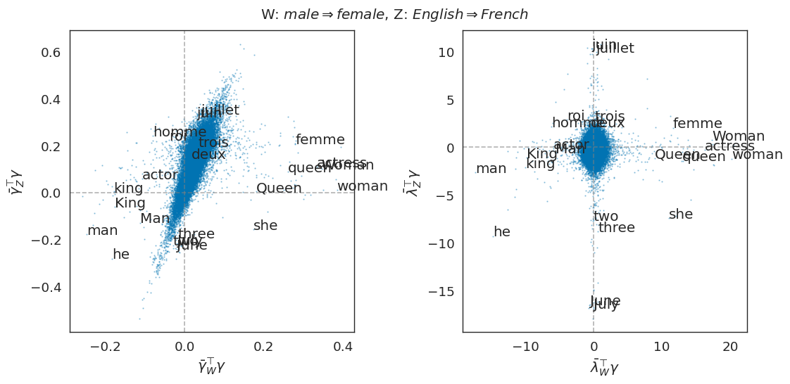
Figure 6: $\bar{\lambda}_{W}^{\top}\gamma$ and $\bar{\lambda}_{Z}^{\top}\gamma$ are independent for the causally separable concepts $W=$male$\Rightarrow$female and $Z=$English$\Rightarrow$French. The plot of $\bar{\gamma}_{W}^{\top}\gamma$ and $\bar{\gamma}_{Z}^{\top}\gamma$ shows that the independence is not common.

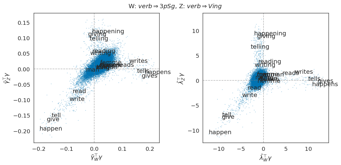
Figure 7: $\bar{\lambda}_{W}^{\top}\gamma$ and $\bar{\lambda}_{Z}^{\top}\gamma$ are not independent for the non-causally separable concepts $W=$verb$\Rightarrow$3pSg and $Z=$verb$\Rightarrow$Ving.

Appendix C Additional Results

C.1 Histograms of random and counterfactual pairs for all concepts

In Figure 8, we include the analog of Figure 2, where we check the causal inner product of the differences between the counterfactual pairs and an LOO estimated unembedding representation for each of the 27 concepts. While the most of the concepts are encoded in the unembedding representation, some concepts, such as thing$\Rightarrow$part, are not encoded in the unembedding space $\Gamma$.

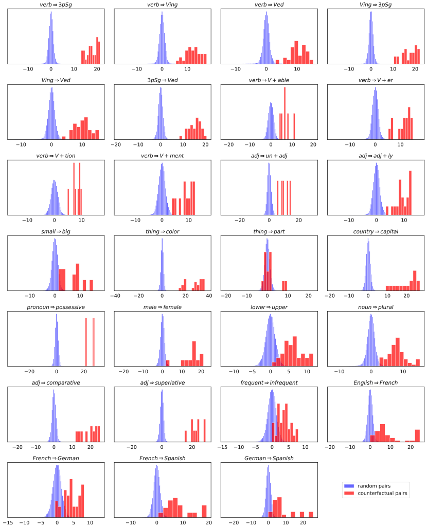
Figure 8: Histograms of the projections of the counterfactual pairs $\langle\bar{\gamma}_{W,(-i)},\gamma(y_{i}(1))-\gamma(y_{i}(0))\rangle_{\mathrm{C}}$ (red), and the projections of 100K randomly sampled word differences $\gamma(Y_{i_{1}})-\gamma(Y_{i_{0}})$ onto the estimated concept direction (blue). Each concept $W$ (the title of each plot) is explained in Table 2.

C.2 Additional results from the measurement experiment

We include the analog of Figure 3, where we use each of the 27 concepts as a linear probe on either French$\Rightarrow$Spanish (Figure 9) or English$\Rightarrow$French (Figure 10) contexts.

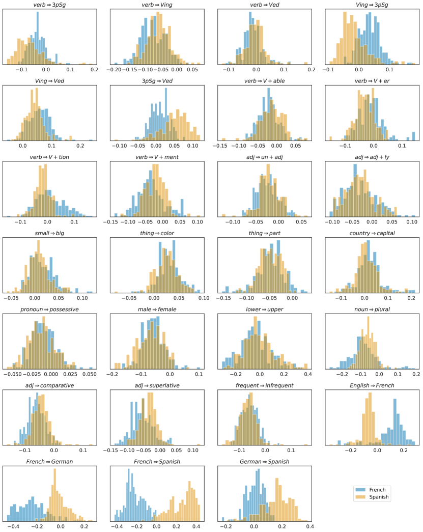
Figure 9: Histogram of $\bar{\gamma}_{C}^{\top}\lambda(x_{j}^{\texttt{fr}})$ vs $\bar{\gamma}_{C}^{\top}\lambda(x_{j}^{\texttt{es}})$ for all concepts $C$, where $\{x_{j}^{\texttt{fr}}\}$ are random contexts from French Wikipedia, and $\{x_{j}^{\texttt{es}}\}$ are random contexts from Spanish Wikipedia.

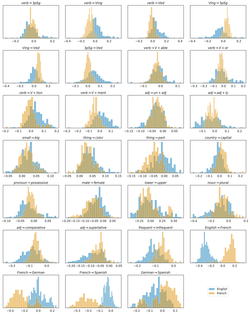
Figure 10: Histogram of $\bar{\gamma}_{C}^{\top}\lambda(x_{j}^{\texttt{en}})$ vs $\bar{\gamma}_{C}^{\top}\lambda(x_{j}^{\texttt{fr}})$ for all concepts $C$, where $\{x_{j}^{\texttt{en}}\}$ are random contexts from English Wikipedia, and $\{x_{j}^{\texttt{fr}}\}$ are random contexts from French Wikipedia.

C.3 Additional results from the intervention experiment

In Figure 11, we include the analog of Figure 4, where we add the embedding representation $\alpha\bar{\lambda}_{C}$ (4.2) for each of the 27 concepts to $\lambda(x_{j})$ and see the change in logits.

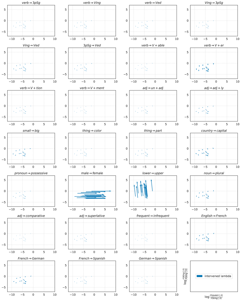
Figure 11: Change in $\log(\mathbb{P}(\text{``queen''}\leavevmode\nobreak\ |\leavevmode\nobreak\ x)/\mathbb{P}(\text{``king''}\leavevmode\nobreak\ |\leavevmode\nobreak\ x))$ and $\log(\mathbb{P}(\text{``King''}\leavevmode\nobreak\ |\leavevmode\nobreak\ x)/\mathbb{P}(\text{``king''}\leavevmode\nobreak\ |\leavevmode\nobreak\ x))$, after changing $\lambda(x_{j})$ to $\lambda_{C,\alpha}(x_{j})$ for $\alpha\in[0,0.4]$ and any concept $C$. The starting point and ending point of each arrow correspond to the $\lambda(x_{j})$ and $\lambda_{C,0.4}(x_{j})$, respectively.

References

- [AB17] Guillaume Alain and Yoshua Bengio “Understanding intermediate layers using linear classifier probes” In International Conference on Learning Representations, 2017 URL: https://openreview.net/forum?id=ryF7rTqgl
- [Aro+16] Sanjeev Arora et al. “A latent variable model approach to PMI-based word embeddings” In Transactions of the Association for Computational Linguistics 4, 2016, pp. 385–399
- [Bel22] Yonatan Belinkov “Probing classifiers: Promises, shortcomings, and advances” In Computational Linguistics 48.1 MIT Press, 2022, pp. 207–219
- [Bow+16] Samuel R. Bowman et al. “Generating Sentences from a Continuous Space” In Proceedings of the 20th SIGNLL Conference on Computational Natural Language Learning Berlin, Germany: Association for Computational Linguistics, 2016, pp. 10–21 DOI: 10.18653/v1/K16-1002
- [CTB22] Tyler Chang, Zhuowen Tu and Benjamin Bergen “The Geometry of Multilingual Language Model Representations” In Proceedings of the 2022 Conference on Empirical Methods in Natural Language Processing, 2022, pp. 119–136
- [Che+21] Boli Chen et al. “Probing BERT in Hyperbolic Spaces” In International Conference on Learning Representations, 2021
- [CCCP20] Hsiao-Yu Chiang, Jose Camacho-Collados and Zachary Pardos “Understanding the source of semantic regularities in word embeddings” In Proceedings of the 24th Conference on Computational Natural Language Learning, 2020, pp. 119–131
- [CPK20] Yo Joong Choe, Kyubyong Park and Dongwoo Kim “word2word: A Collection of Bilingual Lexicons for 3,564 Language Pairs” In Proceedings of the Twelfth Language Resources and Evaluation Conference, 2020, pp. 3036–3045
- [DGM16] Aleksandr Drozd, Anna Gladkova and Satoshi Matsuoka “Word embeddings, analogies, and machine learning: Beyond king - man + woman = queen” In Proceedings of COLING 2016, the 26th International Conference on Computational Linguistics: Technical papers, 2016, pp. 3519–3530
- [Elh+22] Nelson Elhage et al. “Toy Models of Superposition” In arXiv preprint arXiv:2209.10652, 2022
- [Elh+21] Nelson Elhage et al. “A mathematical framework for transformer circuits” In Transformer Circuits Thread 1, 2021
- [Eth19] Kawin Ethayarajh “How Contextual are Contextualized Word Representations? Comparing the Geometry of BERT, ELMo, and GPT-2 Embeddings” In Proceedings of the 2019 Conference on Empirical Methods in Natural Language Processing and the 9th International Joint Conference on Natural Language Processing (EMNLP-IJCNLP), 2019, pp. 55–65
- [FDD20] Louis Fournier, Emmanuel Dupoux and Ewan Dunbar “Analogies minus analogy test: measuring regularities in word embeddings” In Proceedings of the 24th Conference on Computational Natural Language Learning Online: Association for Computational Linguistics, 2020, pp. 365–375 DOI: 10.18653/v1/2020.conll-1.29
- [Gev+22] Mor Geva, Avi Caciularu, Kevin Wang and Yoav Goldberg “Transformer Feed-Forward Layers Build Predictions by Promoting Concepts in the Vocabulary Space” In Proceedings of the Conference on Empirical Methods in Natural Language Processing, 2022, pp. 30–45
- [GDM16] Anna Gladkova, Aleksandr Drozd and Satoshi Matsuoka “Analogy-based detection of morphological and semantic relations with word embeddings: what works and what doesn’t.” In Proceedings of the NAACL Student Research Workshop, 2016, pp. 8–15
- [GL14] Yoav Goldberg and Omer Levy “word2vec Explained: deriving Mikolov et al.’s negative-sampling word-embedding method” In arXiv preprint arXiv:1402.3722, 2014
- [GT23] Wes Gurnee and Max Tegmark “Language Models Represent Space and Time” In arXiv preprint arXiv:2310.02207, 2023, pp. arXiv:2310.02207 DOI: 10.48550/arXiv.2310.02207
- [HGG23] Roee Hendel, Mor Geva and Amir Globerson “In-Context Learning Creates Task Vectors” In arXiv preprint arXiv:2310.15916, 2023
- [Her+23] Evan Hernandez et al. “Linearity of relation decoding in transformer language models” In arXiv preprint arXiv:2308.09124, 2023
- [HM19] John Hewitt and Christopher D Manning “A structural probe for finding syntax in word representations” In Proceedings of the 2019 Conference of the North American Chapter of the Association for Computational Linguistics: Human Language Technologies, Volume 1 (Long and Short Papers), 2019, pp. 4129–4138
- [Hig+18] Irina Higgins et al. “Towards a definition of disentangled representations” In arXiv preprint arXiv:1812.02230, 2018
- [Hig+16] Irina Higgins et al. “beta-VAE: Learning basic visual concepts with a constrained variational framework” In International Conference on Learning Representations, 2016
- [HM16] Aapo Hyvarinen and Hiroshi Morioka “Unsupervised feature extraction by time-contrastive learning and nonlinear ICA” In Advances in Neural Information Processing Systems 29, 2016
- [JAV23] Yibo Jiang, Bryon Aragam and Victor Veitch “Uncovering Meanings of Embeddings via Partial Orthogonality” In arXiv preprint arXiv:2310.17611, 2023
- [Khe+20] Ilyes Khemakhem, Diederik Kingma, Ricardo Monti and Aapo Hyvarinen “Variational autoencoders and nonlinear ICA: A unifying framework” In International Conference on Artificial Intelligence and Statistics, 2020, pp. 2207–2217 PMLR
- [Kim+18] Been Kim et al. “Interpretability beyond feature attribution: Quantitative testing with concept activation vectors (TCAV)” In International Conference on Machine Learning, 2018, pp. 2668–2677 PMLR
- [KR18] Taku Kudo and John Richardson “SentencePiece: A simple and language independent subword tokenizer and detokenizer for Neural Text Processing” In Proceedings of the 2018 Conference on Empirical Methods in Natural Language Processing: System Demonstrations, 2018, pp. 66–71
- [Lam+18] Guillaume Lample et al. “Word translation without parallel data” In International Conference on Learning Representations, 2018
- [LG14] Omer Levy and Yoav Goldberg “Linguistic regularities in sparse and explicit word representations” In Proceedings of the Eighteenth Conference on Computational Natural Language Learning, 2014, pp. 171–180
- [Li+20] Bohan Li et al. “On the Sentence Embeddings from Pre-trained Language Models” In Proceedings of the 2020 Conference on Empirical Methods in Natural Language Processing (EMNLP), 2020, pp. 9119–9130
- [Li+22] Kenneth Li et al. “Emergent World Representations: Exploring a Sequence Model Trained on a Synthetic Task” In International Conference on Learning Representations, 2022
- [Men+22] Kevin Meng, David Bau, Alex Andonian and Yonatan Belinkov “Locating and editing factual associations in GPT” In Advances in Neural Information Processing Systems 35, 2022, pp. 17359–17372
- [MEP23] Jack Merullo, Carsten Eickhoff and Ellie Pavlick “Language Models Implement Simple Word2Vec-style Vector Arithmetic” In arXiv preprint arXiv:2305.16130, 2023
- [MLS13] Tomas Mikolov, Quoc V Le and Ilya Sutskever “Exploiting similarities among languages for machine translation” In arXiv preprint arXiv:1309.4168, 2013
- [Mik+13] Tomas Mikolov et al. “Distributed representations of words and phrases and their compositionality” In Advances in Neural Information Processing Systems 26, 2013
- [MYZ13] Tomáš Mikolov, Wen-Tau Yih and Geoffrey Zweig “Linguistic regularities in continuous space word representations” In Proceedings of the 2013 Conference of the North American Chapter of the Association for Computational Linguistics: Human Language Technologies, 2013, pp. 746–751
- [MT17] David Mimno and Laure Thompson “The strange geometry of skip-gram with negative sampling” In Proceedings of the 2017 Conference on Empirical Methods in Natural Language Processing Copenhagen, Denmark: Association for Computational Linguistics, 2017, pp. 2873–2878 DOI: 10.18653/v1/D17-1308
- [Mor+21] Gemma E. Moran, Dhanya Sridhar, Yixin Wang and David M. Blei “Identifiable Deep Generative Models via Sparse Decoding” In arXiv preprint arXiv:2110.10804, 2021, pp. arXiv:2110.10804 DOI: 10.48550/arXiv.2110.10804
- [NLW23] Neel Nanda, Andrew Lee and Martin Wattenberg “Emergent linear representations in world models of self-supervised sequence models” In arXiv preprint arXiv:2309.00941, 2023
- [nos20] nostalgebraist “Interpreting GPT: the logit lens”, 2020 URL: https://www.alignmentforum.org/posts/AcKRB8wDpdaN6v6ru/interpreting-gpt-the-logit-lens
- [Ope23] OpenAI “GPT-4 Technical Report” In arXiv preprint arXiv:2303.08774, 2023
- [Pen+22] Xutan Peng, Mark Stevenson, Chenghua Lin and Chen Li “Understanding Linearity of Cross-Lingual Word Embedding Mappings” In Transactions on Machine Learning Research, 2022 URL: https://openreview.net/forum?id=8HuyXvbvqX
- [PSM14] Jeffrey Pennington, Richard Socher and Christopher D Manning “GloVe: Global vectors for word representation” In Proceedings of the 2014 Conference on Empirical Methods in Natural Language Processing (EMNLP), 2014, pp. 1532–1543
- [Per+23] Pramuditha Perera et al. “Prompt Algebra for Task Composition” In arXiv preprint arXiv:2306.00310, 2023
- [Rad+18] Alec Radford, Karthik Narasimhan, Tim Salimans and Ilya Sutskever “Improving language understanding by generative pre-training” OpenAI, 2018
- [Rei+19] Emily Reif et al. “Visualizing and measuring the geometry of BERT” In Advances in Neural Information Processing Systems 32, 2019
- [RKR21] Anna Rogers, Olga Kovaleva and Anna Rumshisky “A primer in BERTology: What we know about how BERT works” In Transactions of the Association for Computational Linguistics 8 MIT Press, 2021, pp. 842–866
- [RVS19] Sebastian Ruder, Ivan Vulić and Anders Søgaard “A survey of cross-lingual word embedding models” In Journal of Artificial Intelligence Research 65, 2019, pp. 569–631
- [Sch+21] Bernhard Schölkopf et al. “Toward causal representation learning” In Proceedings of the IEEE 109.5 IEEE, 2021, pp. 612–634
- [Tod+23] Eric Todd et al. “Function Vectors in Large Language Models” In arXiv preprint arXiv:2310.15213, 2023
- [Tou+23] Hugo Touvron et al. “Llama 2: Open foundation and fine-tuned chat models” In arXiv preprint arXiv:2307.09288, 2023
- [Tra+23] Matthew Trager et al. “Linear spaces of meanings: Compositional structures in vision-language models” In Proceedings of the IEEE/CVF International Conference on Computer Vision, 2023, pp. 15395–15404
- [Tur+23] Alexander Matt Turner et al. “Activation Addition: Steering Language Models Without Optimization” In arXiv preprint arXiv:2308.10248, 2023, pp. arXiv:2308.10248 DOI: 10.48550/arXiv.2308.10248
- [Ush+21] Asahi Ushio, Luis Espinosa Anke, Steven Schockaert and Jose Camacho-Collados “BERT is to NLP what AlexNet is to CV: Can Pre-Trained Language Models Identify Analogies?” In Proceedings of the 59th Annual Meeting of the Association for Computational Linguistics and the 11th International Joint Conference on Natural Language Processing (Volume 1: Long Papers), 2021, pp. 3609–3624
- [Vas+17] Ashish Vaswani et al. “Attention is all you need” In Advances in Neural Information Processing Systems 30, 2017
- [Vyl+16] Ekaterina Vylomova, Laura Rimell, Trevor Cohn and Timothy Baldwin “Take and Took, Gaggle and Goose, Book and Read: Evaluating the Utility of Vector Differences for Lexical Relation Learning” In Proceedings of the 54th Annual Meeting of the Association for Computational Linguistics (Volume 1: Long Papers), 2016, pp. 1671–1682
- [Wan+23] Zihao Wang, Lin Gui, Jeffrey Negrea and Victor Veitch “Concept Algebra for Score-Based Conditional Models” In arXiv preprint arXiv:2302.03693, 2023
- [ZM20] Xunjie Zhu and Gerard Melo “Sentence analogies: Linguistic regularities in sentence embeddings” In Proceedings of the 28th International Conference on Computational Linguistics, 2020, pp. 3389–3400
- [Zim+21] Roland S Zimmermann et al. “Contrastive learning inverts the data generating process” In International Conference on Machine Learning, 2021, pp. 12979–12990 PMLR
- [Zou+23] Andy Zou et al. “Representation Engineering: A Top-Down Approach to AI Transparency” In arXiv preprint arXiv:2310.01405, 2023