The detection of polarized x-ray emission from the magnetar 1E 2259+586

Abstract

We report on IXPE, NICER and XMM-Newton observations of the magnetar 1E 2259+586. We find that the source is significantly polarized at about or above 20% for all phases except for the secondary peak where it is more weakly polarized. The polarization degree is strongest during the primary minimum which is also the phase where an absorption feature has been identified previously (Pizzocaro et al., 2019). The polarization angle of the photons are consistent with a rotating vector model with a mode switch between the primary minimum and the rest of the rotation of the neutron star. We propose a scenario in which the emission at the source is weakly polarized (as in a condensed surface) and, as the radiation passes through a plasma arch, resonant cyclotron scattering off of protons produces the observed polarized radiation. This confirms the magnetar nature of the source with a surface field greater than about $10^{15}$ G.

1 Introduction

Gregory & Fahlman (1980) discovered the X-ray source 1E 2259+586 in observations of the supernova remnant G109.l$-$1.0 using the Einstein telescope on 17 December 1979. Later identified as one of the Anomalous X-ray Pulsars (AXPs; Mereghetti & Stella, 1995), 1E 2259+586 was the first member of this class to be discovered (and the third magnetar after SGR 1806$-$20 and SGR 0525$-$66 earlier in 1979). Fahlman & Gregory (1981) identified a periodicity in the X-ray emission from the source of 3.4890 s. Subsequent observations revealed that the pulse profile exhibits two similar peaks over each rotation period. Similar to the other anomalous X-ray pulsars the spin period of 1E 2259+586 is gradually increasing ($\dot{P}\approx 5\times 10^{-13}$ s s^-1, Dib & Kaspi, 2014), and this is associated with the presence of a strong magnetic field ($\approx 6\times 10^{13}$ G) and the braking of the pulsar through magnetic dipole radiation. Although the dipole magnetic field inferred from the spin down lies at the low end of the magnetar range (in fact several radio pulsars have larger spin-down fields, Manchester et al., 2005), 1E 2259+586 exhibits bursts, glitches and even an anti-glitch similar to other magnetars (Kaspi & Beloborodov, 2017), suggesting that a much stronger field of $10^{14}$–$10^{15}$ G, confined in small scale structures close to the surface, is present in 1E 2259+586, similarly to the other “low-field” magnetar SGR 0418+5729 (Tiengo et al., 2013).

Pizzocaro et al. (2019) found evidence of phase-dependent spectral features in XMM-Newton observations of 1E 2259+586 that have been consistent in phase and energy over more than a decade while the source has been in quiescence. On the other hand, during an active epoch in 2002, although the spectral feature was still present, its position in energy as a function of phase had changed. Pizzocaro et al. (2019) proposed that this feature could be a signature of resonant cyclotron scattering similar to what has been proposed for a similar feature found in the phase-resolved spectrum of SGR 0418+5729 (Tiengo et al., 2013). If this association is correct in the case of 1E 2259+586, the magnetic field for a proton cyclotron resonance is $(3-16)\times 10^{14}$ G (and below $10^{12}$ G for an electron cyclotron resonance). Here we present polarimetric observations that provide evidence that this spectral feature results from photons scattering off of non-relativistic particles (most likely protons) at the cyclotron resonance.

2 Observations

IXPE observed 1E 2259+5586 in June–July 2023 and a simultaneous XMM-Newton pointing was carried out on June 30 2023. NICER archival data, partially overlapping the IXPE time window, were also available. Tab. 1 summarizes the observations used for this analysis.

Table 1: Observation Log.

Obs ID	MJD${}_{\textrm{Start}}$	Exposure [s]
IXPE
02007899	60098	1202835
NICER
6533040201	60022	358
6533040301	60036	834
6533040401	60050	1271
6533040402	60064	1790
6533040601	60078	698
6533040701	60107	565
6533040901	60120	541
6533041001	60134	776
6533041101	60149	564
XMM-Newton
0744800101	56868	112000
0931790401	60126	20500

2.1 IXPE

IXPE, a NASA mission in partnership with the Italian space agency (ASI; Weisskopf et al., 2022, and references therein) observed 1E 2259+5861 on 2023 June 2–19 and June 30–July 6 for 1.2 Ms in total. The gas-pixel detectors on IXPE register the arrival time, sky position, and energy for each X-ray photon and use the photoelectric effect to provide an estimate of the position angle of each photon (Soffitta et al., 2021). During each observation, photon arrival events registered between energies of $2$ and $8$ keV, within $48$ arcseconds of the position of source (R.A. $=345^{\circ}.3$, DEC $=58^{\circ}.9$), were extracted for analysis. The background was estimated from an annular region centered on the source of inner and outer radii of $78$ arcseconds and $240$ arcseconds, respectively. Background subtraction was applied to the extracted Stokes parameters. Anyway, we observe that the background level for each IXPE detector unit (DU, i.e. telescope) in the $2$–$8$ keV band was less than $2\%$ of the source one. We could, hence, conclude that the energy-integrated analysis we performed is not much affected by background effects. The times of the photon arrivals were finally corrected for the motion of IXPE around the barycenter of the Solar System.

2.2 NICER

We used the Neutron star Interior Composition Explorer (NICER; Gendreau et al., 2012; LaMarr et al., 2016; Prigozhin et al., 2016) data collected over 2023 March 19 to 2023 July 24. The data were processed with HEASoft version 6.31 and NICER Data Analysis Software (NICER-DAS) version 10 (2022-12-16_V010a) using the nicerl2 tool with standard filtering criteria, resulting in 6.1 ks of filtered exposure. We performed barycenter corrections in the ICRS reference frame using the JPL DE421 Solar System ephemeris with the barycorr tool in FTOOLS with coordinates ${\rm R.A.}=345\aas@@fstack{\circ}2845$, ${\rm DEC}=58\aas@@fstack{\circ}879$.

2.3 XMM-Newton

A DDT pointing of 1E 2259+586 with XMM-Newton was activated on 2023, June 30, starting at 23:47:46 UTC for an exposure time of $\approx 20$ ks. The EPIC-pn (Strüder et al., 2001) as well as the two MOS cameras (Turner et al., 2001) were set in the Small Window mode, with a time resolution of $0.3$ s. Row data were processed by means of the SAS version 20.0 and the most updated calibration files. After the subtraction of the intervals in which the background events were dominant, the data were extracted and processed applying standard procedures, for a net exposure of $\approx 19.1$ ks for the MOSs and $\approx 18.8$ ks for the EPIC-pn. We extracted the source counts from a circular region of radius about 65". Those of the background were extracted from a similar region, within the same CCD where the source lies and $\sim$2.5’ away for the pn, while for the MOSs, due to the use of the small window mode, from another CCD (at a distance of about 9’ from the source). The times of the extracted photons were corrected for the barycenter of the Solar System in the ICRS reference frame with barycen tool in the SAS. The background subtracted source count rates were 10.71(3) ct s^-1 in the pn and 3.31(1) in the MOSs (1$\sigma$ confidence levels are reported).

3 Results

3.1 Timing analysis

We first started analysing the datasets from each missions. In order to estimate the most reliable timing solution for the $1.2$ Ms exposure IXPE dataset, we used a phase-fitting approach (see, for example, Dall’Osso et al., 2003) which gave a period of $6.979281(1)$ s, or $\nu=0.14328124(3)$ Hz, at the reference epoch of 60097.0 MJD (a further $\dot{P}$ component did not significantly improve the fit). The peak-to-peak semi-amplitude of the background subtracted light curves folded to the above period resulted to be $(33\pm 3)\%$. For NICER, the same phase-fitting algorithm revealed that a quadratic component was significantly present in the spin period phases as a function of time, resulting in the following timing solution: $P=6.9792783(1)$s and $\dot{P}=5.0(2)\times 10^{-13}$ s s^-1, reference epoch 60022.0 MJD (1$\sigma$ confidence levels are reported), corresponding to $\nu=0.143281290(3)$ Hz and $\dot{\nu}=-1.03(4)\times 10^{-14}$ Hz s^-1. Similarly, for XMM-Newton the best timing solution was inferred to be $P=6.97931(2)$ s or $\nu=0.1432806(4)$ Hz at reference epoch 60126.0 MJD. The inclusion of a first period derivative $\dot{P}$ did not significantly improve the fit. The peak-to-peak semi-amplitude of the background subtracted light curves folded to the above period resulted to be (35$\pm$3)%. Note that the three timing solutions are in agreement with each other within their uncertainties. Finally, the whole sample of IXPE, NICER and XMM-Newton datasets was used simultaneously to provide the best possible timing solution. A phase-fitting analysis (see Figure 1) gave the following result, $P=6.9792785(1)$s and $\dot{P}=4.7(1)\times 10^{-13}$ s s^-1, reference epoch 60022.0 MJD, corresponding to $\nu=0.143281286(2)$ Hz and $\dot{\nu}=-9.7(3)\times 10^{-15}$ Hz s^-1 (1$\sigma$ c.l.; reduced $\chi^{2}$$\sim$2 for 14 d.o.f. and rms of 0.007 cycles). In Figure 2 we show the light curves of each mission folded to the best solution discussed above. The pulse shape is double peaked and does not change, within uncertainties, considering different energy bands. Figure 3 shows the IXPE pulse profile with the different phase ranges used in the subsequent analysis: Big Dip, Rise, Big Peak, Little Dip and Little Peak (see Section 4 for further details); phase zero was chosen to coincide with that of Pizzocaro et al. (2019).

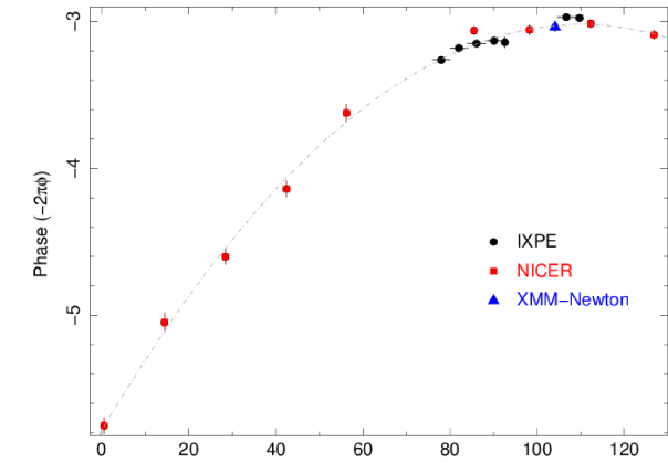
MMMTime [days since MJD 60022.0]

Figure 1: 1E 2259+586 phase evolution (in radian units) as a function of time fitted with a linear plus a quadratic component for the whole data sample used in the analysis, that includes IXPE (black filled circles), NICER (red filled squares) and XMM-Newton (blue filled triangles). The dash-dotted line marks the best fit.

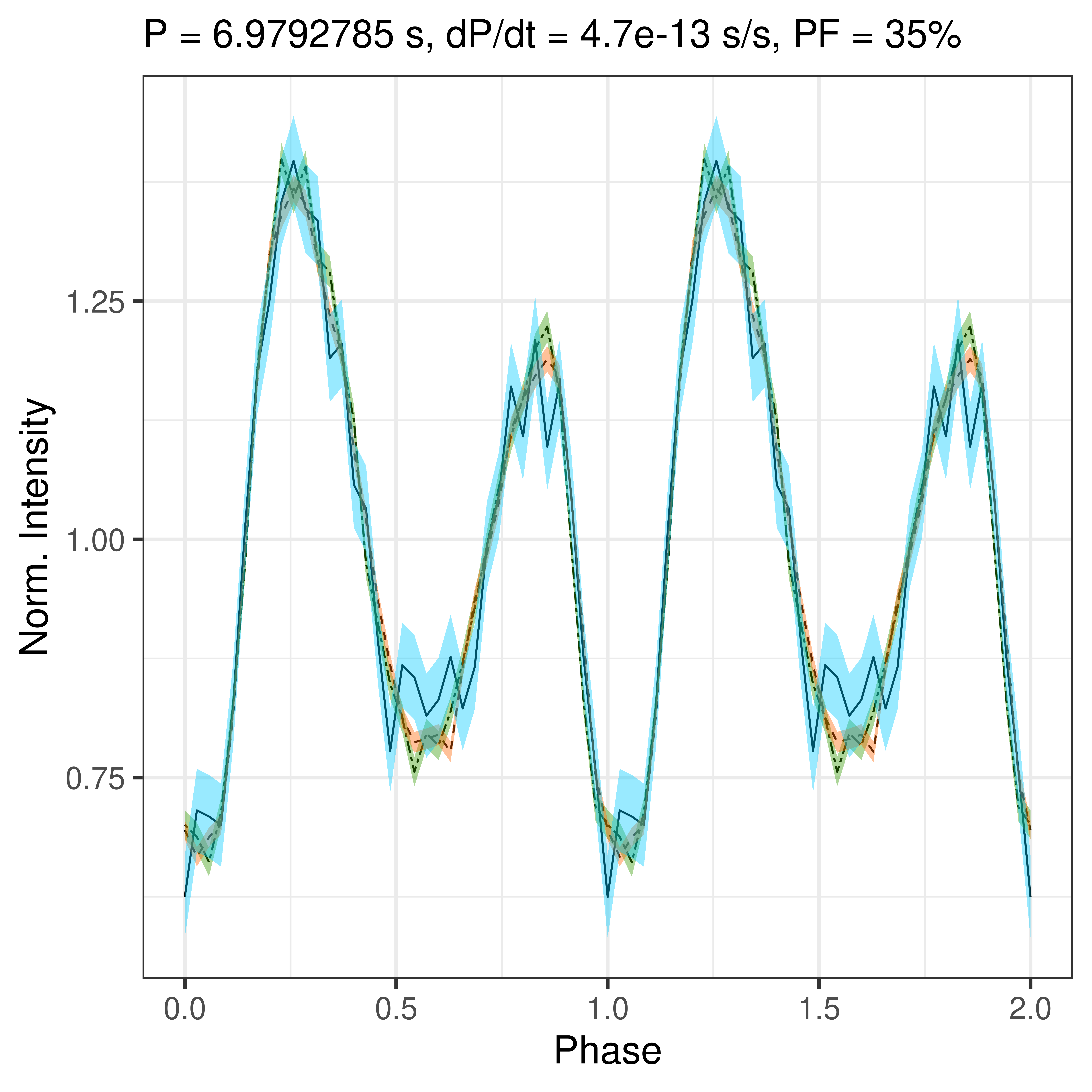
Figure 2: $1$–$10$ keV NICER (cyan), $1$–$10$ keV XMM-Newton (green) and $2$–$8$ keV IXPE (orange) light curves folded to the best timing solution inferred from the whole sample of datasets and discussed in section 3.1 (see also Figure 1).

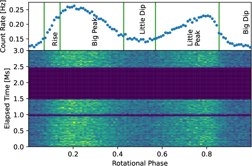
Figure 3: IXPE Counts as a function of rotational phase and elapsed time for the inferred values of spin frequency and frequency derivative (see text for details). The zero phase and reference time are at MJD 60097.966874079. The spectral analysis phase regions are delineated and named in the upper panel (the Big Dip region spans across phase zero).

3.2 Spectral analysis

We first performed a phase-integrated spectral analysis of the XMM-Newton observation by fitting simultaneously the EPIC-pn and MOS data in the $0.5$–$8$ keV energy range using XSPEC (Arnaud, 1996). Fits with (absorbed) single-component models (either a blackbody, BB, or a power-law, PL) turned out to be rather unsatisfactory, with a reduced $\chi^{2}$ exceeding $6$ for $250$ degrees of freedom (dof). A substantial improvement was obtained adding a second component. A purely thermal model (BB+BB), however, still resulted in a poor fit, with $\chi^{2}=462.2$ for 248 dof and a temperature for the hotter blackbody of $\sim 300$ keV, difficult to reconcile with the known properties of magnetars (see e.g. Turolla et al., 2015; Kaspi & Beloborodov, 2017, for reviews). By adopting a BB+PL decomposition the fit improved, although it was still far from being statistically acceptable, and the best-fitting parameters are compatible with those presented in previous works Zhu et al. (2008); Pizzocaro et al. (2019). The addition of a Gaussian absorption line, (gabs in XSPEC, as in Pizzocaro et al., 2019), resulted in a further improvement in the quality of the fit ($\chi^{2}=341.0$ for $245$ dof). By performing an f-test, the probability that the additional absorption line is unnecessary turns out to be $4.3\times 10^{-7}$ (i.e. the feature is significant at $\sim 5\sigma$ confidence level). The corresponding BB temperature, PL photon index, line energy and width are in agreement with those reported in Pizzocaro et al. (2019) within $1\sigma$ confidence level (see Table 2 for the fit parameters). The large $\chi^{2}$ for the pn+MOS fit indicates that fitting the merged dataset to the phase-average spectrum may be inadequate. Indeed, by restricting to the EPIC-pn data only resulted in a much better fit ($\chi^{2}=94.1$ for $93$ dof for the same spectral model, see Figure 4), although the line centroid shifted to slightly higher energies. Results of the phase-resolved spectroscopic analysis are presented in Section 5.

We finally attempted a fit of the IXPE $2$–$8$ keV data using the same spectral decomposition and freezing the column density and line parameters to those obtained from the fit of the EPIC-pn data. The fit is statistically acceptable ($\chi^{2}=138.0$ for 147 dof) with values of the free parameters in agreement (within statistical uncertainties) with those already obtained in the previous analyses (see again Table 2 and Figure 4).

Table 2: Results of the phase-integrated spectral fits with the model phabs$\times$(bbodyrad+powerlaw)$\times$gabs.

Data	$N_{\mathrm{H}}$	$kT_{{\rm BB}}$	$R_{{\rm BB}}\,^{a}$	$\Gamma_{\rm PL}$	NormPL at $1$ keV	$E_{\rm abs}$	$\sigma_{\rm abs}$	Depthabs	$\chi^{2}$/dof
	[$10^{22}\,\mathrm{cm}^{-2}$]	[keV]	[km]		[$10^{-3}$/s/keV/cm2]	[keV]	[keV]	[keV]
PN+MOS	$0.91^{+0.08}_{-0.13}$	$0.446^{+0.008}_{-0.009}$	2.24${}^{+0.13}_{-0.13}$	$3.93^{+0.08}_{-0.11}$	$50.72^{+6.87}_{-9.14}$	$0.71\pm^{+0.17}_{-0.22}$	$0.30^{+0.09}_{-0.08}$	$0.30^{+0.63}_{-0.20}$	$341.0/245$
PN	$1.02^{+0.03}_{-0.07}$	$0.437^{+0.012}_{-0.011}$	$2.33^{+0.22}_{-0.21}$	$4.09^{+0.08}_{-0.08}$	$62.09^{+6.81}_{-6.41}$	$0.96^{+0.07}_{-0.18}$	$0.23^{+0.10}_{-0.06}$	$0.11^{+0.20}_{-0.05}$	$94.1/93$
IXPE$\,{}^{b}$	$1.02\,^{c}$	$0.429^{+0.011}_{-0.010}$	$2.45^{+0.24}_{-0.20}$	$4.36^{+0.09}_{-0.09}$	$75.95^{+7.79}_{-7.80}$	$0.96\,^{c}$	$0.23\,^{c}$	$0.11\,^{c}$	$138.0/147$

• Errors are at $1\sigma$ confidence level.

• Derived by adopting a $3.2$ kpc distance (Kothes & Foster, 2012; Pizzocaro et al., 2019).

• For fitting IXPE data the spectral decomposition was convolved with a constant factor to take into account the different calibration of the 3 DUs (the relative calibration factors obtained from the fit are compatible with those found in previous magnetar analyses, see Taverna et al., 2022; Zane et al., 2023; Turolla et al., 2023).

• Frozen to the value obtained from the PN fit.

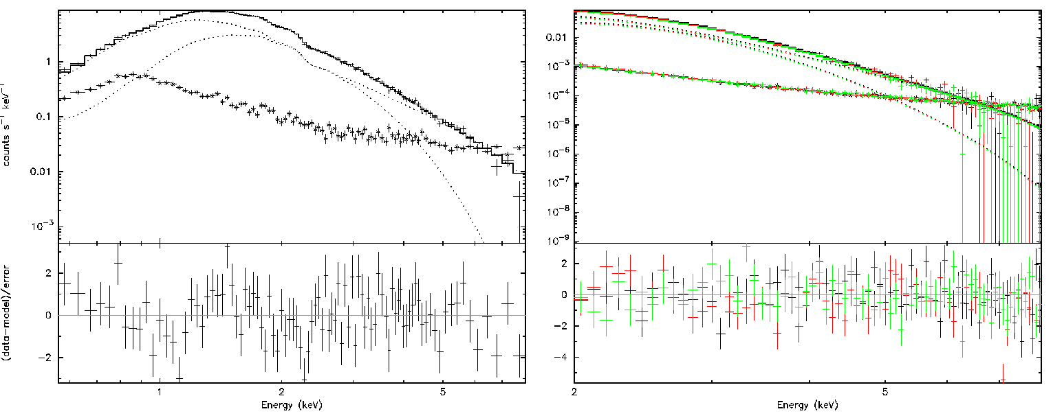
Figure 4: Left: spectral fit of the EPIC-pn XMM-Newton data with the phabs$\times$(bbodyrad+powerlaw)$\times$gabs model in the $0.5$–$8$ keV range. Right: same for the IXPE DU1 (black), DU2 (red) and DU3 (green) data in the $2$–$8$ keV range. The single spectral components are marked by dotted lines (see also Table 2) and the background counts by crosses with error bars.

3.3 Polarization analysis

A phase- and energy-integrated study (in the $2$–$8$ keV band) of the polarization properties of the source was performed using the PCUBE algorithm of the ixpeobssim suite Baldini et al. (2022). The results for the normalized Stokes parameters $Q/I$ and $U/I$ are reported in Figure 5 for the single IXPE DUs and for the sum of them. In the figure the loci of constant polarization degree (PD $=\sqrt{(Q/I)^{2}+(U/I)^{2}}$) and polarization angle (PA $=\arctan(U/Q)/2$) are also shown, together with the value of the minimum detectable polarization at $99\%$ confidence level (MDP₉₉; Weisskopf et al., 2010). We obtained a highly probable detection (significance $>99.9\%$), with PD $=5.6\pm 1.4\%$ (above the MDP${}_{99}=4.5\%$) and PA $=-75^{\circ}.2\pm 7^{\circ}.4$ measured East of North (errors at $1\sigma$).

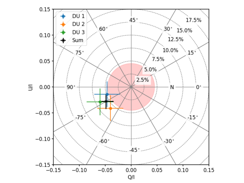
Figure 5: Normalized Stokes parameters $Q/I$ and $U/I$ (filled circles with $1\sigma$ error bars) averaged over the rotational phase and integrated in the $2$–$8$ keV energy band for the single IXPE DUs (cyan, orange and green, respectively) for the sum (black). The gray-dotted circles represents the levels of constant PD, while the gray-solid lines those of constant PA (measured East of North). The red shaded region represents the MDP at $99\%$ confidence level for the combined measurement.

We performed a phase-integrated, energy-dependent polarimetric analysis as well, by dividing the $2$–$8$ keV band into 3 bins. The only bin with a polarization degree in excess of the MDP₉₉ is that at low energies ($2.0$–$3.2$ keV), with PD $=6.1\pm 1.5\%$ (MDP${}_{99}=4.6\%$) and PA $=-66^{\circ}.4\pm 7^{\circ}.1$ (errors at $1\sigma$). In the rest of the energy range we can derive only upper limits: PD $<14.6\%$ in the $3.2$–$5.0$ keV range and PD $<70.0\%$ in the $5.0$–$8.0$ keV one, at $3\sigma$ confidence level. However, the null hypothesis probability that no polarization is detected is below $3\times 10^{-4}$.

In order to study the evolution of the polarization with the rotational phase, we divided the counts into 14 equally spaced phase bins taking as phase zero the one reported in Pizzocaro et al. (2019). In each bin we calculate the normalized Stokes parameters $Q/I$ and $U/I$ using the likelihood method outlined in González-Caniulef et al. (2023); similar results can be achieved using the standard tools (e.g. ixpeobssim). The results are given in Table 3. There (as well as in the central panel of Figure 7) we listed the values of polarization degree and polarization angle even for the bins where the PD lies below the $\textrm{MDP}_{99}$. This is justified because we measured an overall polarization with high significance (see above), so that the null hypothesis relevant here is not that of unpolarized radiation, but rather of constant polarization. This allows us to probe the agreement between the binned results and the polarization models which are fit directly to the data for individual photons (González-Caniulef et al., 2023).

The Stokes parameters for the bins reported in Table 3 are also shown in Fig. 6. There, three distinct regimes in phase can be recognized. The polarized flux is maximized during the Big Dip (the cluster at the top of Figure 6) and the Big Peak (the cluster at the bottom left). The polarized flux during the Little Dip is modest, and the polarized flux in the Little Peak and the Rise is very low.

Table 3: The normalized Stokes parameters, polarization degree and angle (2$-$8 keV) for the IXPE observation of 1E 2259+5861 in the different phase bins. The uncertainties correspond to $\Delta\log L=1/2$ contours of the likelihood (González-Caniulef et al., 2023).

N	Phase Range	$Q/I$	$U/I$	$\textrm{MDP}_{99}$	PD	PA [deg]	Counts	Region
1	$0.000-0.071$	$0.002\pm 0.054$	$0.225\pm 0.052$	0.163	$0.225\pm 0.051$	$44.7\pm~{}~{}6.9$	11443	Big Dip
2	$0.071-0.143$	$0.040\pm 0.045$	$0.021\pm 0.045$	0.135	$0.045\pm 0.041$	$13.9\pm 27.7$	16962	Rise
3	$0.143-0.214$	$-0.119\pm 0.039$	$-0.064\pm 0.039$	0.118	$0.136\pm 0.036$	$-75.8\pm~{}~{}8.1$	21788	Big Peak
4	$0.214-0.286$	$-0.140\pm 0.039$	$-0.105\pm 0.039$	0.118	$0.175\pm 0.037$	$-71.6\pm~{}~{}6.3$	21445	Big Peak
5	$0.286-0.357$	$-0.151\pm 0.041$	$-0.167\pm 0.042$	0.126	$0.225\pm 0.039$	$-66.1\pm~{}~{}4.9$	18739	Big Peak
6	$0.357-0.429$	$-0.086\pm 0.047$	$-0.099\pm 0.046$	0.141	$0.131\pm 0.044$	$-65.4\pm~{}~{}9.8$	15111	Big Peak
7	$0.429-0.500$	$-0.146\pm 0.049$	$-0.167\pm 0.050$	0.150	$0.222\pm 0.050$	$-65.6\pm~{}~{}6.1$	12988	Little Dip
8	$0.500-0.571$	$-0.013\pm 0.050$	$-0.127\pm 0.051$	0.153	$0.128\pm 0.049$	$-47.9\pm 10.5$	12589	Little Dip
9	$0.571-0.643$	$0.020\pm 0.049$	$0.011\pm 0.048$	0.145	$0.023\pm 0.050$	$14.2\pm 57.0$	14039	Little Peak
10	$0.643-0.714$	$-0.025\pm 0.045$	$0.013\pm 0.046$	0.136	$0.029\pm 0.045$	$76.3\pm 32.5$	16426	Little Peak
11	$0.714-0.786$	$0.098\pm 0.042$	$-0.022\pm 0.042$	0.126	$0.100\pm 0.041$	$-6.4\pm 11.4$	18709	Little Peak
12	$0.786-0.857$	$0.018\pm 0.043$	$-0.042\pm 0.043$	0.130	$0.045\pm 0.042$	$-33.1\pm 26.5$	18389	Little Peak
13	$0.857-0.929$	$0.036\pm 0.052$	$0.194\pm 0.051$	0.156	$0.197\pm 0.050$	$39.7\pm~{}~{}7.2$	12495	Big Dip
14	$0.929-1.000$	$-0.072\pm 0.055$	$0.247\pm 0.054$	0.165	$0.257\pm 0.053$	$53.1\pm~{}~{}5.8$	10920	Big Dip

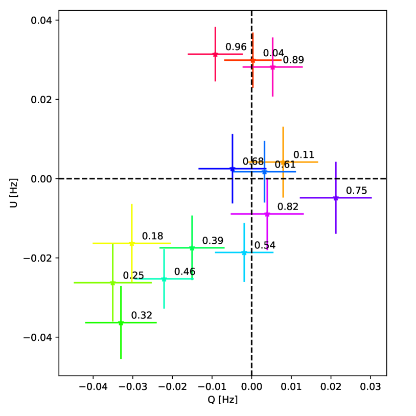
Figure 6: The Stokes Parameters $Q$ and $U$ as a function of phase in units of the mean number of counts per second observed with IXPE in the $2$–$8$ keV range. The uncertainties correspond to $\Delta\log L=1/2$ contours of the likelihood. Each cross is labeled by the central value of the corresponding phase bin and coloured according to phase starting with red at phase zero and proceeding along the colour wheel through green then blue.

4 Polarization Modeling

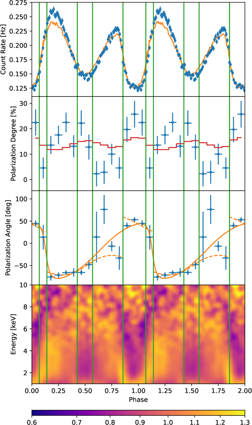
Figure 7: IXPE and XMM-Newton energy-integrated ($2$–$8$ keV range) counts (upper), PD (upper-center) and PA (lower and lower-center, blue points with error bars). The uncertainties in the lower panels correspond to $\Delta\log L=1/2$ contours of the likelihood. The orange curve in the upper panel is the XMM-Newton ($0.3$–$12$ keV) pulse profile from Pizzocaro et al. (2019) scaled to the mean count rate of IXPE. The red curve in the second panel depicts the value of MDP₉₉ for each bin. The orange curves in the third panel show the best-fitting RVM model without (solid) or with (dashed) mode switching The lowermost panel shows the phase-resolved spectrum observed in 2014 with XMM-Newton EPIC-pn (as in Fig. 2 of Pizzocaro et al., 2019), normalized to the phase-averaged energy spectrum and energy-integrated pulse profile. The vertical green lines mark the five phase intervals used in our analysis.

In the highly magnetized environment surrounding a magnetar radiation propagates into two (normal) modes, the ordinary (O) and extraordinary (X) ones. In the former case, the electric field of the wave oscillates in the plane of the (local) magnetic field and of the photon momentum, while in the latter the oscillations are perpendicular to this plane (Gnedin et al., 1978; Pavlov & Shibanov, 1979). Even in the absence of matter, vacuum birefringence will force the polarization vector of photons to follow the direction of the (local) magnetic field until the so-called polarization-limiting radius (Heyl & Shaviv, 2000, 2002). For typical magnetars, this radius is estimated to be about $200$–$300$ stellar radii for keV photons (see, e.g., Figure 1 of Taverna et al., 2015, and also Heyl & Caiazzo 2018), where the field is dominated by the dipole component. The polarization measured at the telescope is, then, expected to be either parallel or perpendicular to the instantaneous projection of the magnetic dipole axis of the star onto the plane of the sky. For this reason, the modulation of the polarization angle with phase is decoupled from the evolution of the polarization degree and intensity (that carry the imprint of the conditions at emission) and most likely should follow the rotating vector model (RVM; Radhakrishnan & Cooke, 1969; Poutanen, 2020, see also Taverna et al. 2022; González-Caniulef et al. 2023),

$$\tan(\textrm{PA}-\chi_{\rm p})=\frac{\sin\theta\sin(\phi-\phi_{0})}{\cos i_{\rm p}\sin\theta\cos(\phi-\phi_{0})-\sin i_{\rm p}\cos\theta},$$ (1)

where $i_{\rm p}$ is the inclination of the spin axis with respect to the line-of-sight, $\chi_{\rm p}$ the position angle of the spin axis in the plane of the sky (measured East of North), $\theta$ the inclination of the magnetic axis to the spin axis and $\phi$ is the spin phase ($\phi_{0}$ is the initial phase). The angle between the dipole axis and the line-of-sight varies between $i_{\rm p}-\theta$ at $\phi=\phi_{0}$ and $i_{\rm p}+\theta$ at $\phi=\phi_{0}+\pi$. Without loss of generality we restrict the parameters as follows:

$$0\leq i_{\rm p}\leq 180^{\circ},0\leq\theta\leq 90^{\circ},0\leq\chi_{\rm p}<180^{\circ},0\leq\phi_{0}<360^{\circ}.$$

The two best-fitting RVMs for the polarization angle are depicted in Figure 7. The solid curve traces a model where the polarization mode is constant with phase, and the dashed curve shows a model where the polarization mode switches at a phase where the polarization degree is low. This is accomplished by replacing the Stokes parameters ($Q$ and $U$) of the model by their additive inverse over a range of phases $\phi_{1}<\phi<\phi_{2}$ where $\phi_{1}$ and $\phi_{2}$ are two additional parameters. The log-likelihood of the first model (with $\textrm{PD}=11.6\%$) is 49.6 and that of the second one ($\textrm{PD}=12.7\%$) is 57.8. The log-likelihoods for 222,043 events, drawn from two models with the observed values of PDs, are distributed approximately normally, with means of $48$ and $56$ and standard deviations of $10$; this indicates that both models are good fits to the data; about 60% of the time random events drawn from these models will yield likelihoods smaller than those measured for the data. Figure 8 depicts posterior distributions of the parameters for these two models.

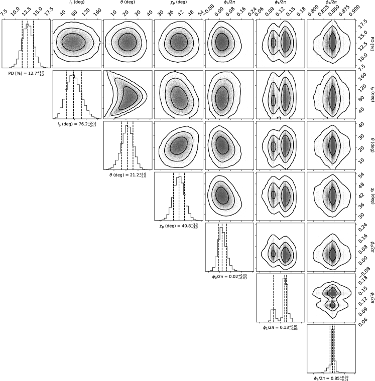
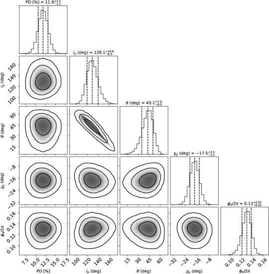
Figure 8: Posteriors of the RVM for the IXPE observations of 1E 2259+5586 The two-dimensional contours correspond to $68\%$, $95\%$ and $99\%$ confidence levels. The histograms show the normalized one-dimensional distributions for a given parameter derived from the posterior samples. The upper grid depicts constraints on the RVM with a mode switch between phases $\phi_{1}$ and $\phi_{2}$. The lower grid depicts the constraints on the RVM without a mode switch.

Table 4: Best-fitting RVM parameters. When the data are consistent with the model, the log-likelihood ($\log L$) is normally distributed. The fit quality in the last column is given in terms of the best-fitting log-likelihood compared with the expected value, where positive values indicate better-than-expected values.

	Mean PD	$\chi_{\rm p}$	$\theta$	$i_{\rm p}$	$\phi_{0}/2\pi$	$\phi_{1}/2\pi$	$\phi_{2}/2\pi$	$\Delta\log L$
	[%]	[deg]	[deg]	[deg]				[$\sigma$]
Mode-Switching Model	$12.7\pm 1.2$	$\!~{}~{}~{}76.2^{+27.2}_{-24.7}$	$21.2^{+4.6}_{-5.0}$	$~{}~{}~{}40.8\pm 3.3$	$0.02\pm 0.02$	$0.13^{+0.01}_{-0.03}$	$0.85\pm 0.01$	$+0.18$
Single-Mode Model	$11.9\pm 1.2$	$129.1^{+10.6}_{-9.3}$	$43.1^{+7.0}_{-8.5}$	$-17.5\pm 3.1$	$0.13\pm 0.01$	—	—-	$\!+0.16$

As the model without mode switching is nested within the mode-switching model, we can calculate the probability to achieve the measured likelihood ratio even if there is no mode switch (the null hypothesis). Twice the difference in likelihoods is distributed as a $\chi^{2}$ distribution with two degrees of freedom (for the two additional parameters), yielding a probabilty that the null hypothesis is true of less than $3\times 10^{-4}$. Furthermore, one of the mode switches can account for the low polarization at phase 0.11 that lies between two high polarization regimes. Figure 9 examines the single-mode RVM in more detail by removing the effect of the motion of the magnetic axis on the plane of the sky from the measured photon polarization angles. To this aim, the $Q$ and $U$ Stokes parameters for each photon are rotated into the frame of the best-fitting RVM before measuring the polarization angle and degree. If the low polarization at phase 0.11 results from the smearing of a large intrinsic polarization as the star rotates, the polarization measured after this procedure would be large. However, as Figure 9 shows, the polarization at this phase remains low, so it is indeed a natural time for a mode switch as found in the mode-switching model indicated by dashed lines in Figure 7. Both the single-mode and the mode-switching models allow for solutions with $i_{\rm p}>90^{\circ}$ such that the dipole axis points closest toward the line-of-sight (and so the emission is expected to be brighter, Heyl & Hernquist, 1998) at phase 0.13 and 0.02, respectively, landing just before the Big Peak of the light curve. For $i_{\rm p}<90^{\circ}$, a secondary peak lies at about phase zero. However, it is obvious from Figure 7 that phase zero is the deepest minimum in the light curve. Beyond the mode switching itself, a key difference between the models is that the model without mode switching requires the angle between the magnetic axis and the spin axis ($\theta$) to be larger ($43^{\circ}$) than what is expected for the mode-switching model ($21^{\circ}$), in order to account for the observed swing in polarization angle between the Big Dip and the Big Peak. In the mode switching model, this is accomplished with a smaller magnetic obliquity plus a mode switch at phases 0.1 and 0.85, so during the Big Dip the emission is dominated by a different polarization mode than the rest of the time.

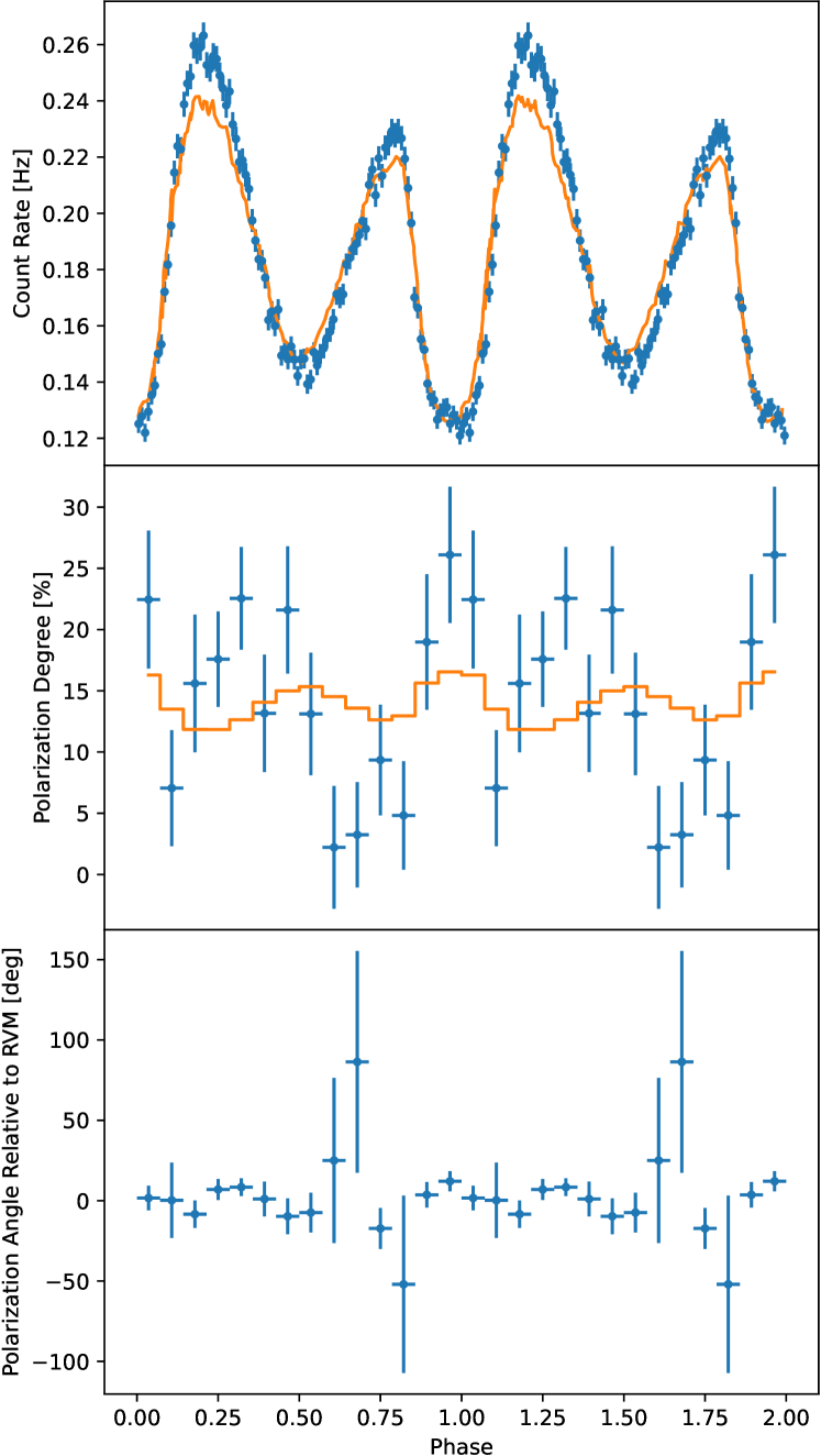
Figure 9: Same as in the upper, upper-center and lower-center panels of Figure 7, but with Stokes parameters referred to the frame of the best-fitting RVM without mode switching. The polarization angles are generally consistent with zero within the uncertainties, while the polarization degree is similar to that shown in Figure 7, except for phase 0.1, during the rapid swing in the RVM, where the polarization is somewhat washed out in Figure 7. However, even when correcting for the rotation, the polarization degree at this phase lies below MDP₉₉.

In the mode-switching model the emission should peak right in the middle of the Big Dip, if it is associated with the orientation of the dipole field. If one ignores the phase region of the Big Dip, the rest of the pulse profile can result from a single hot spot about $10^{\circ}$ in radius located about $20^{\circ}$ from the spin axis, and with the spin axis pointing about $100^{\circ}$ from the line-of-sight (as in Figure 8). These considerations, along with the unique polarization signature of the Big Dip, point toward the hypothesis that the basic emission geometry of the pulsar is straightforward with some sort of obscuration that operates during the Big Dip.

Pizzocaro et al. (2019) found evidence for a spectral feature around phase zero (the Big Dip) that appears consistently in XMM-Newton observations of 1E 2259+586 in quiescence in 2002 and again in 2014. When the source was in outburst in 2002, a feature appears but with a different phase dependence. The pulse profile that we have observed with IXPE is consistent with that observed with XMM-Newton in 2014, as shown in the upper panel of Figure 7. The lowermost panel of Figure 7 depicts the phase-resolved spectrum of 1E 2259+586 in 2014, indicating the presence of the spectral feature coincident with the large dip in the pulse profile of the source. This is further highlighted in Figure 10, where the $2$–$8$ keV, phase-resolved spectra for the XMM-Newton 2014 and 2023 observations are shown together with the IXPE one. Although the signal-to-noise ratio of the shorter 2023 observations is lower than that of the 2014 ones, the absorption feature is discernible both in the IXPE and the latest XMM-Newton observations as well.

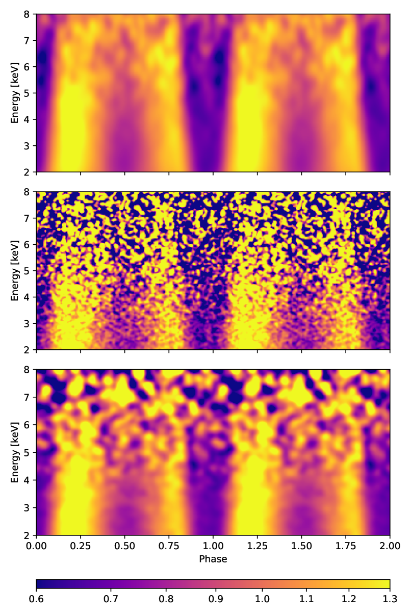
Figure 10: Phase-resolved spectra of 1E 2259+586 in the $2$–$8$ keV range as observed by XMM-Newton EPIC-pn in 2014 (upper panel, as in Fig. 3 of Pizzocaro et al., 2019), by XMM-Newton EPIC-pn and MOS in 2023 (middle panel), and by IXPE in 2023 (lower panel). These are normalized to the phase-averaged energy spectrum but not normalized to the energy-integrated pulse profile.

Pizzocaro et al. (2019) argue that this feature may be due to resonant cyclotron scattering of X-rays off of protons in the magnetosphere. In analogy to the results of Tiengo et al. (2013), the scattering plasma should be confined along a magnetic loop above the surface, with proton cyclotron energy ranging from about $2$ to $10$ keV, corresponding to a magnetic field strength along the loop from $3\times 10^{14}$ G to $2\times 10^{15}$ G, neglecting gravitational redshift.

To examine the implications of this scenario on the polarized flux from the surface of the neutron star, we adapt the expressions for electron resonant cyclotron scattering cross sections in the non-relativistic limit Nobili et al. (2008) to the case of scattering off protons,

$$\begin{array}[]{lll}\dfrac{\textrm{d}\sigma}{\textrm{d}\Omega}_{\textrm{O}\rightarrow\textrm{O}}&=&\dfrac{3\pi r_{0}c}{8}\delta(\omega-\omega_{B})\cos^{2}\beta\cos^{2}\beta^{\prime}\\ &&\\ \dfrac{\textrm{d}\sigma}{\textrm{d}\Omega}_{\textrm{O}\rightarrow\textrm{X}}&=&\dfrac{3\pi r_{0}c}{8}\delta(\omega-\omega_{B})\cos^{2}\beta\\ &&\\ \dfrac{\textrm{d}\sigma}{\textrm{d}\Omega}_{\textrm{X}\rightarrow\textrm{X}}&=&\dfrac{3\pi r_{0}c}{8}\delta(\omega-\omega_{B})\\ &&\\ \dfrac{\textrm{d}\sigma}{\textrm{d}\Omega}_{\textrm{X}\rightarrow\textrm{O}}&=&\dfrac{3\pi r_{0}c}{8}\delta(\omega-\omega_{B})\cos^{2}\beta^{\prime}\,,\end{array}$$ (2)

where $\beta$ ($\beta^{\prime}$) is the photon angle with respect to the magnetic field before (after) scattering, $\omega$ is the photon frequency, $\omega_{B}$ is the proton cyclotron frequency and $r_{0}$ is the classical proton radius (a factor of 1,836 smaller than that of the electron). On the left-hand sides, the first (second) subscript indicates the polarization mode of the incoming (scattered) photon. A key feature of this scattering process is that the ordinary mode photons are less likely to scatter (by a factor of three for an isotropic radiation field), and the photon after scattering is three times more likely to be in the extraordinary mode, regardless of the polarization of the incoming photon. Consequently, if the absorption feature evident in the XMM-Newton observations is due to resonant cyclotron scattering, the radiation that passes through the plasma without scattering will be dominated by O-mode photons.

To illustrate this, let us assume that the count rate at phase zero in the absence of scattering is 0.275 Hz, and the radiation before scattering is unpolarized. The rate of scattered photons is 0.150 Hz (from the decrease in flux during the Big Dip as observed by IXPE); so, if the rate of scattering of extraordinary and ordinary photons is 0.090 Hz and 0.060 Hz, respectively (to total 0.150 Hz), the unscattered radiation that we observe at phase zero would have $U=0.030$ Hz (dominated by the ordinary mode) and a polarization degree of about $25\%$, as observed. A modest difference in the scattering probability of $50\%$ in this example is sufficient to account for the observed polarization in the minimum. Two thirds of the scattered photons emerge in the extraordinary mode and one third in the ordinary mode, so over the three phase bins, where the scattering occurs, a net of 0.05 photons per second are scattered into the extraordinary mode (i.e $\textrm{O}\rightarrow\textrm{X}$). If we assume that these are visible over the five phase bins from 0.18 to 0.46, the average rate is 0.03 Hz, as observed in these phases at the corresponding polarization angle, if the dominant mode does indeed switch from ordinary to extraordinary at about phase 0.1. The presence of scattered photons in the Big Peak can account for the observed polarization at this phase of the star’s rotation. On the other hand, the Little Peak is not appreciably polarized and is somewhat smaller in amplitude; both these features are expected if the scattered photons do not contribute at this phase. In principle the plasma loop is simply hidden behind the star during the Little Peak until its footprints appear over the horizon at the beginning of the Big Dip and the loop begins to block our line-of-sight to the emission region. Clearly, this scenario requires a complicated geometry for the magnetic field near the surface that does not correspond to the large-scale dipole field of the neutron star. This should in principle rule out an explanation of the observed polarization angle in terms of a simple RVM. The fact that the RVM does indeed provide a reliable explanation to the data is further evidence that the polarization direction is determined at a distance far away from the surface (i.e. the polarization-limited radius), where the field and therefore the polarization vectors are aligned with the global dipole direction.

5 Spectropolarimetric Modelling

We next examine the extent of polarization averaged over the rotational phase as a function of energy. In order to get a better sense of the polarization properties at the emission, the polarization angles of the photons at each phase are measured relative to the best-fitting RVM (with mode switching, the dashed curve in the third panel of Figure 7). The results are reported in Figure 11. In particular the values of $U/I$ are consistent with zero which reflects the fact that the polarization states of the photons are conserved as the photons travel out to the polarization-limiting radius (Heyl & Shaviv, 2000). If there were a substantial source of polarized emission outside the polarization-limiting radius, the value of $U/I$ would not necessarily vanish. The component of polarization along and across the dipole axis ($Q/I$) ranges from near $20\%$ at $2$ keV and drops to be essentially consistent with zero above $4$ keV. This dovetails with the hypothesis that the observed polarization is generated by resonant cyclotron scattering off of protons, as the proton cyclotron line lies at lower energies in the middle of the Big Dip where the polarization is strongest.

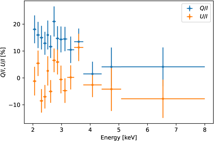
Figure 11: Normalized Stokes parameters $Q/I$ and $U/I$ plotted as functions of energy, referred to the frame of the best-fitting RVM with mode switching (dashed curve in Figure 7).

We further examine the energy dependence of the polarization as a function of phase. We focus on just the two regions with large polarized fractions, the Big Dip and the Big Peak and on a relatively narrow range in energy, because the number of photons turns out to be insufficient to reliably determine the polarization above $2.6$ keV in these phase intervals. The results are shown in Figure 12. In both the regions considered, we find that the values of $U/I$ are consistent with zero, as expected. The polarization degree in the Big Dip (upper panel) is essentially constant across the band, indicating that an equal fraction of photons are scattered as a function of energy. Since the spectral feature is broad (see the bottom panel of Figure 7 and Section 5.1), this is not surprising. On the other hand, the lower panel of Figure 12 shows that the polarization degree decreases with energy and is consistent with zero above $2.3$ keV. This feature can also be explained in the scattering picture after we better understand the spectral components as a function of phase (see Section 3.2).

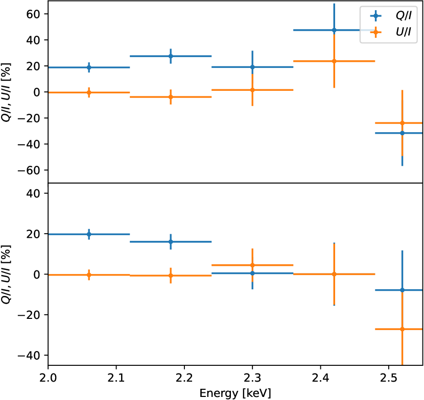
Figure 12: Same as in Figure 11 but for the Big Dip (upper panel) and the Big Peak (lower panel) phase intervals, restricted to the $2$–$2.6$ keV range. Both $Q$ and $U$ are measured relative to the best-fitting RVM.

To gain further understanding of the spectral behaviour of the source, we performed the same spectral fitting within each of the phase bins defined in Figure 3 and Table 3. We also fit the 2023 XMM-Newton EPIC-pn spectra within these bins with and without an absorption feature (the results are reported in Table 5). The fits with and without the feature yield acceptable $\chi^{2}$ values for the Big Dip and Little Dip, with fits with the spectral feature being preferred. However, for the Big Peak and Little Peak, the fits without the spectral feature are unacceptable. Interestingly, during the Rise, where, according to Figure 7, the line is quickly changing in energy, neither fit is acceptable. In all of the fits, the energy of the spectral line is about $1$ keV, with a width about $0.2$ keV and a depth $\approx 0.15$ keV. The emission during the Big Peak is typically harder than in the Big Dip. We found that the fraction of scattered photons during the Big Dip was approximately constant with energy (upper panel of Figure 12). If these photons are preferentially scattered into the extraordinary mode, the contribution of the scattered photons at another phase will be largest where the spectrum of incoming photons is largest. Because the Big Dip is relatively softer than the Big Peak, the relative contribution of the scattered photons to the observed flux will be larger at lower energies, resulting in a decrease of the polarization degree with energy (lower panel of Figure 12).

Table 5: Results of phase-dependent spectral modelling of the XMM-Newton EPIC-pn data using the phabs$\times$(bbodyrad+powerlaw) and phabs$\times$(bbodyrad+powerlaw)$\times$gabs decompositions$\,{}^{a}$.

Region	$kT_{\textrm{BB}}$	$R_{\textrm{BB}}$b	$\Gamma_{\textrm{PL}}$	$\textrm{Norm}_{\textrm{PL}}$ at 1 keV	$E_{\textrm{abs}}$	$\sigma_{\textrm{abs}}$	Depth${}_{\textrm{abs}}$	$\chi^{2}/\textrm{dof}$
	[keV]	[km]		[$10^{-3}$/s/keV/cm2]	[keV]	[keV]	[keV]
Big Dip	$0.431_{-0.014}^{+0.014}$	$1.87_{-0.18}^{+0.18}$	$4.15_{-0.07}^{+0.08}$	$39.0_{-2.1}^{+3.0}$	$1.07_{-0.06}^{+0.08}$	$0.15_{-0.07}^{+0.08}$	$0.05_{-0.03}^{+0.05}$	75.8 / 78
	$0.411_{-0.010}^{+0.010}$	$2.30_{-0.13}^{+0.15}$	$3.95_{-0.06}^{+0.06}$	$29.2_{-0.8}^{+0.8}$	—	—	—	80.9 / 81
Rise	$0.401_{-0.026}^{+0.034}$	$2.49_{-0.62}^{+0.59}$	$4.28_{-0.15}^{+0.19}$	$64.7_{-8.5}^{+2.1}$	$0.96_{-0.13}^{+0.08}$	$0.25_{-0.10}^{+0.16}$	$0.16_{-0.10}^{+0.36}$	73.4 / 63
	$0.373_{-0.013}^{+0.013}$	$3.55_{-0.29}^{+0.35}$	$3.98_{-0.07}^{+0.08}$	$40.8_{-1.7}^{+1.6}$	—	—	—	77.3 / 66
Big Peak	$0.423_{-0.011}^{+0.011}$	$2.26_{-0.16}^{+0.17}$	$3.90_{-0.04}^{+0.04}$	$54.0_{-2.0}^{+2.4}$	$1.06_{-0.03}^{+0.03}$	$0.14_{-0.04}^{+0.04}$	$0.05_{-0.02}^{+0.02}$	106.1 / 103
	$0.402_{-0.007}^{+0.007}$	$2.89_{-0.13}^{+0.14}$	$3.71_{-0.03}^{+0.03}$	$39.7_{-0.8}^{+0.8}$	—	—	—	122.9 / 106
Little Dip	$0.476_{-0.037}^{+0.048}$	$1.00_{-0.25}^{+0.29}$	$3.94_{-0.08}^{+0.11}$	$38.1_{-3.3}^{+6.2}$	$1.10_{-0.10}^{+0.08}$	$0.25_{-0.09}^{+0.13}$	$0.11_{-0.06}^{+0.17}$	71.2 / 78
	$0.435_{-0.018}^{+0.018}$	$1.55_{-0.14}^{+0.18}$	$3.74_{-0.05}^{+0.06}$	$27.0_{-0.7}^{+0.7}$	—	—	—	74.3 / 81
Little Peak	$0.407_{-0.014}^{+0.015}$	$2.23_{-0.26}^{+0.26}$	$3.91_{-0.04}^{+0.06}$	$56.0_{-3.1}^{+5.1}$	$1.09_{-0.05}^{+0.04}$	$0.19_{-0.05}^{+0.07}$	$0.08_{-0.03}^{+0.06}$	103.5 / 100
	$0.393_{-0.008}^{+0.008}$	$2.90_{-0.15}^{+0.16}$	$3.70_{-0.03}^{+0.03}$	$39.1_{-0.8}^{+0.8}$	—	—	—	122.3 / 103

• Errors are at $1\sigma$ confidence level.

• The column density parameter is frozen to that returned by the correspondent best fitting model of the phase-integrated EPIC-pn data (see section 3.2), i.e. $N_{\rm H}=0.96\times 10^{22}\,{\rm cm}^{-2}$ and $1.02\times 10^{22}\,{\rm cm}^{-2}$, respectively.

• Derived by adopting a $3.2$ kpc distance (Kothes & Foster, 2012; Pizzocaro et al., 2019).

5.1 The spectral feature

We define the region in energy and phase containing the spectral feature as centred on

$$E=12.3~{}\textrm{keV}-\frac{11.9~{}\textrm{keV}}{1+78.4x^{2}}\,,$$ (3)

where

$$x=\left\{\frac{\phi}{2\pi}-0.971+\frac{1}{2}\right\}-\frac{1}{2}$$ (4)

and $\{\}$ denotes the fractional part and $\phi$ is the rotational phase in radians. We take the width of the feature to be $2$ keV. The particular numerical values in equations (3) and (4) were determined by finding the region of width $2$ keV with the smallest mean value of the phase-resolved spectrum normalized by the phase-averaged energy spectrum and then by the energy-integrated pulse profile (the upper middle panel of Figure 13). By design, the mean at each phase is unity. For the XMM-Newton observation, the standard deviation of the mean over a region with the area delineated in the upper panel is 0.01, whereas the value obtained in the XMM-Newton energy-phase region is 0.86 (fourteen standard deviations below the expected value). For IXPE in the similarly sized region the standard deviation is 0.005 and the value obtained is 0.88 (twenty-four standard deviations below the expected value), indicating with high confidence that the spectral feature is also present in the recent IXPE observations. The upper most panel of Figure 13 depicts the response of a filter with the shape of the feature against the three datasets. In all three the feature is detected with the matched filter.

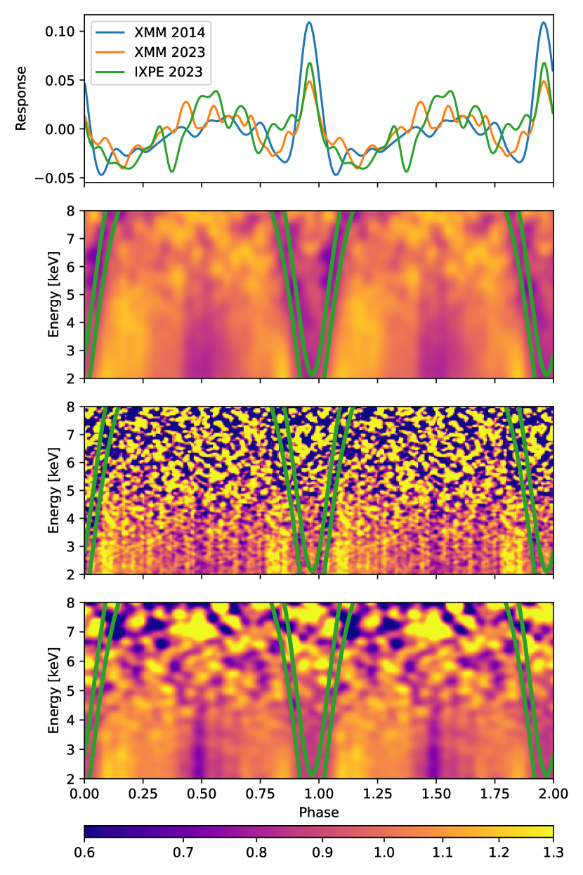
Figure 13: Dynamic Phase- and Energy-Normalized Spectra. Upper: Response using a matched filter defined by the line detected in the XMM-Newton 2014 EPIC-pn data when applied to the XMM-Newton EPIC-pn data from 2014, EPIC-pn and MOS data from 2023, and the IXPE data in 2023. The response finds the line feature in all three datasets centered at about the phase 0.97. Upper-Middle: the dynamic spectrum from XMM-Newton EPiC-pn in 2014 with the defined feature region from Eq. 3 superimposed. Lower-Middle: the dynamic spectrum from XMM-Newton EPIC-pn and MOS in 2023. Lower: the dynamic spectrum from IXPE in 2023. Both are normalized by the phase-averaged energy spectrum and then the energy-integrated pulse profile (as Fig. 2 of Pizzocaro et al., 2019, and Fig. 7 above).

We can exploit the time and energy-resolution of IXPE to calculate the polarization degree for only the events within the phase and energy domain delineated by equation (3) within the Big Dip phase interval, $(0.86,0.07)$. We obtain $Q/I=0.05\pm 0.06$ and $U/I=0.28\pm 0.06$ (measured relative to North, with $\textrm{MDP}_{99}=0.18$). If we examine the same phase range and exclude the energy range of the feature, we obtain $Q/I=-0.03\pm 0.04$ and $U/I=0.20\pm 0.04$ (with $\textrm{MDP}_{99}=0.11$), demonstrating that the spectral region defined by the feature in the XMM-Newton observation may be significantly more polarized than the emission at other energies during this phase of the star’s rotation.

6 Conclusions

Observations of 1E 2259+5586 with IXPE and XMM-Newton support a consistent scenario for the emission from this source. According to our interpretation, the emission is initially only weakly polarized as expected for a condensed surface layer as in 4U 0142+61 (Taverna et al., 2022) and 1RXS J170849.0–400910 (Zane et al., 2023), but during particular phases of the star’s rotation the radiation that reaches us passes through a loop of plasma, and protons scatter the radiation in the cyclotron resonance (as in SGR 0418+5729, Tiengo et al., 2013). As the scattering is preferentially from the ordinary mode into the extraordinary mode, this results in a net polarization in the ordinary mode during the phase where the radiation passes through the loop towards us (the Big Dip), and in the extraordinary mode during the phases where the loop is visible but does not intersect the line-of-sight to the emission region (the Big Peak and Little Dip), leaving us to observe scattered photons. During the Little Peak, the polarization is weak, presumably because an emission region with its inherently weak polarization is visible, but the plasma loop is hidden from view, so scattered photons do not contribute during this phase. Further observations of 1E 2259+586 with IXPE could confirm the hint that the polarized flux correlates both in energy and phase with the spectral absorption feature found by Pizzocaro et al. (2019).

Data Availability

The data used for this analysis are available through HEASARC under IXPE Observation ID 02007899.

List of Affiliations

¹ University of British Columbia, Vancouver, BC V6T 1Z4, Canada
² Dipartimento di Fisica e Astronomia, Università degli Studi di Padova, Via Marzolo 8, 35131 Padova, Italy
³ Mullard Space Science Laboratory, University College London, Holmbury St Mary, Dorking, Surrey RH5 6NT, UK
⁴ INAF Osservatorio Astronomico di Roma, Via Frascati 33, 00078 Monte Porzio Catone (RM), Italy
⁵ MIT Kavli Institute for Astrophysics and Space Research, Massachusetts Institute of Technology, 77 Massachusetts Avenue, Cambridge, MA 02139, USA
⁶ Institut de Recherche en Astrophysique et Planétologie, UPS-OMP, CNRS, CNES, 9 avenue du Colonel Roche, BP 44346 31028, Toulouse CEDEX 4, France
⁷ California Institute of Technology, Pasadena, CA 91125, USA
⁸ NASA Marshall Space Flight Center, Huntsville, AL 35812, USA
⁹ Department of Physics and Astronomy, Louisiana State University, Baton Rouge, LA 70803, USA
¹⁰ Instituto de Astrofísica de Andalucía, CSIC, Glorieta de la Astronomía s/n, 18008 Granada, Spain
¹¹ Space Science Data Center, Agenzia Spaziale Italiana, Via del Politecnico snc, 00133 Roma, Italy
¹² INAF Osservatorio Astronomico di Cagliari, Via della Scienza 5, 09047 Selargius (CA), Italy
¹³ Istituto Nazionale di Fisica Nucleare, Sezione di Pisa, Largo B. Pontecorvo 3, 56127 Pisa, Italy
¹⁴ Dipartimento di Fisica, Università di Pisa, Largo B. Pontecorvo 3, 56127 Pisa, Italy
¹⁵ Dipartimento di Matematica e Fisica, Università degli Studi Roma Tre, Via della Vasca Navale 84, 00146 Roma, Italy
¹⁶ Istituto Nazionale di Fisica Nucleare, Sezione di Torino, Via Pietro Giuria 1, 10125 Torino, Italy
¹⁷ Dipartimento di Fisica, Università degli Studi di Torino, Via Pietro Giuria 1, 10125 Torino, Italy
¹⁸ INAF Osservatorio Astrofisico di Arcetri, Largo Enrico Fermi 5, 50125 Firenze, Italy
¹⁹ Dipartimento di Fisica e Astronomia, Università degli Studi di Firenze, Via Sansone 1, 50019 Sesto Fiorentino (FI), Italy
²⁰ Istituto Nazionale di Fisica Nucleare, Sezione di Firenze, Via Sansone 1, 50019 Sesto Fiorentino (FI), Italy
²¹ INAF Istituto di Astrofisica e Planetologia Spaziali, Via del Fosso del Cavaliere 100, 00133 Roma, Italy
²² ASI - Agenzia Spaziale Italiana, Via del Politecnico snc, 00133 Roma, Italy
²³ Science and Technology Institute, Universities Space Research Association, Huntsville, AL 35805, USA
²⁴ Istituto Nazionale di Fisica Nucleare, Sezione di Roma "Tor Vergata", Via della Ricerca Scientifica 1, 00133 Roma, Italy
²⁵ Department of Physics and Kavli Institute for Particle Astrophysics and Cosmology, Stanford University, Stanford, California 94305, USA
²⁶ Institut für Astronomie und Astrophysik, Universität Tübingen, Sand 1, 72076 Tübingen, Germany
²⁷ Astronomical Institute of the Czech Academy of Sciences, Boční II 1401/1, 14100 Praha 4, Czech Republic
²⁸ RIKEN Cluster for Pioneering Research, 2-1 Hirosawa, Wako, Saitama 351-0198, Japan
²⁹ NASA Goddard Space Flight Center, Greenbelt, MD 20771, USA
³⁰ Yamagata University,1-4-12 Kojirakawa-machi, Yamagata-shi 990-8560, Japan
³¹ Osaka University, 1-1 Yamadaoka, Suita, Osaka 565-0871, Japan
³² International Center for Hadron Astrophysics, Chiba University, Chiba 263-8522, Japan
³³ Institute for Astrophysical Research, Boston University, 725 Commonwealth Avenue, Boston, MA 02215, USA
³⁴ Department of Astrophysics, St. Petersburg State University, Universitetsky pr. 28, Petrodvoretz, 198504 St. Petersburg, Russia
³⁵ Department of Physics and Astronomy and Space Science Center, University of New Hampshire, Durham, NH 03824, USA
³⁶ Physics Department and McDonnell Center for the Space Sciences, Washington University in St. Louis, St. Louis, MO 63130, USA
³⁷ Istituto Nazionale di Fisica Nucleare, Sezione di Napoli, Strada Comunale Cinthia, 80126 Napoli, Italy
³⁸ Université de Strasbourg, CNRS, Observatoire Astronomique de Strasbourg, UMR 7550, 67000 Strasbourg, France
³⁹ Graduate School of Science, Division of Particle and Astrophysical Science, Nagoya University, Furo-cho, Chikusa-ku, Nagoya, Aichi 464-8602, Japan
⁴⁰ Hiroshima Astrophysical Science Center, Hiroshima University, 1-3-1 Kagamiyama, Higashi-Hiroshima, Hiroshima 739-8526, Japan
⁴¹ Department of Physics, The University of Hong Kong, Pokfulam, Hong Kong
⁴² Department of Astronomy and Astrophysics, Pennsylvania State University, University Park, PA 16802, USA
⁴³ Université Grenoble Alpes, CNRS, IPAG, 38000 Grenoble, France
⁴⁴ Department of Physics and Astronomy, 20014 University of Turku, Finland
⁴⁵ Center for Astrophysics | Harvard & Smithsonian, 60 Garden St, Cambridge, MA 02138, USA
⁴⁶ INAF Osservatorio Astronomico di Brera, Via E. Bianchi 46, 23807 Merate (LC), Italy
⁴⁷ Dipartimento di Fisica, Università degli Studi di Roma "Tor Vergata", Via della Ricerca Scientifica 1, 00133 Roma, Italy
⁴⁸ Department of Astronomy, University of Maryland, College Park, Maryland 20742, USA
⁴⁹ Anton Pannekoek Institute for Astronomy & GRAPPA, University of Amsterdam, Science Park 904, 1098 XH Amsterdam, The Netherlands
⁵⁰ Guangxi Key Laboratory for Relativistic Astrophysics, School of Physical Science and Technology, Guangxi University, Nanning 530004, China

References

- Arnaud (1996) Arnaud K. A., 1996, in Jacoby G. H., Barnes J., eds, Astronomical Society of the Pacific Conference Series Vol. 101, Astronomical Data Analysis Software and Systems V. p. 17
- Astropy Collaboration et al. (2013) Astropy Collaboration et al., 2013, A&A, 558, A33
- Astropy Collaboration et al. (2018) Astropy Collaboration et al., 2018, AJ, 156, 123
- Astropy Collaboration et al. (2022) Astropy Collaboration et al., 2022, ApJ, 935, 167
- Baldini et al. (2022) Baldini L., et al., 2022, SoftwareX, 19, 101194
- Dall’Osso et al. (2003) Dall’Osso S., Israel G. L., Stella L., Possenti A., Perozzi E., 2003, ApJ, 599, 485
- Dib & Kaspi (2014) Dib R., Kaspi V. M., 2014, ApJ, 784, 37
- Fahlman & Gregory (1981) Fahlman G. G., Gregory P. C., 1981, Nature, 293, 202
- Gendreau et al. (2012) Gendreau K. C., Arzoumanian Z., Okajima T., 2012, in Takahashi T., Murray S. S., den Herder J.-W. A., eds, Society of Photo-Optical Instrumentation Engineers (SPIE) Conference Series Vol. 8443, Space Telescopes and Instrumentation 2012: Ultraviolet to Gamma Ray. p. 844313, doi:10.1117/12.926396
- Gnedin et al. (1978) Gnedin Y. N., Pavlov G. G., Shibanov Y. A., 1978, Soviet Astronomy Letters, 4, 117
- González-Caniulef et al. (2023) González-Caniulef D., Caiazzo I., Heyl J., 2023, MNRAS, 519, 5902
- Gregory & Fahlman (1980) Gregory P. C., Fahlman G. G., 1980, Nature, 287, 805
- Harris et al. (2020) Harris C. R., et al., 2020, Nature, 585, 357
- Heyl & Caiazzo (2018) Heyl J., Caiazzo I., 2018, Galaxies, 6, 76
- Heyl & Hernquist (1998) Heyl J. S., Hernquist L., 1998, MNRAS, 300, 599
- Heyl & Shaviv (2000) Heyl J. S., Shaviv N. J., 2000, MNRAS, 311, 555
- Heyl & Shaviv (2002) Heyl J. S., Shaviv N. J., 2002, Phys. Rev. D, 66, 023002
- Hunter (2007) Hunter J. D., 2007, Computing in Science & Engineering, 9, 90
- Kaspi & Beloborodov (2017) Kaspi V. M., Beloborodov A. M., 2017, ARA&A, 55, 261
- Kothes & Foster (2012) Kothes R., Foster T., 2012, ApJ, 746, L4
- LaMarr et al. (2016) LaMarr B., Prigozhin G., Remillard R., Malonis A., Gendreau K. C., Arzoumanian Z., Markwardt C. B., Baumgartner W. H., 2016, in den Herder J.-W. A., Takahashi T., Bautz M., eds, Society of Photo-Optical Instrumentation Engineers (SPIE) Conference Series Vol. 9905, Space Telescopes and Instrumentation 2016: Ultraviolet to Gamma Ray. p. 99054W, doi:10.1117/12.2232784
- Manchester et al. (2005) Manchester R. N., Hobbs G. B., Teoh A., Hobbs M., 2005, AJ, 129, 1993
- Mereghetti & Stella (1995) Mereghetti S., Stella L., 1995, ApJ, 442, L17
- Nobili et al. (2008) Nobili L., Turolla R., Zane S., 2008, MNRAS, 386, 1527
- Pavlov & Shibanov (1979) Pavlov G. G., Shibanov Y. A., 1979, Soviet Journal of Experimental and Theoretical Physics, 49, 741
- Pizzocaro et al. (2019) Pizzocaro D., et al., 2019, A&A, 626, A39
- Poutanen (2020) Poutanen J., 2020, A&A, 641, A166
- Prigozhin et al. (2016) Prigozhin G., et al., 2016, in den Herder J.-W. A., Takahashi T., Bautz M., eds, Society of Photo-Optical Instrumentation Engineers (SPIE) Conference Series Vol. 9905, Space Telescopes and Instrumentation 2016: Ultraviolet to Gamma Ray. p. 99051I, doi:10.1117/12.2231718
- Radhakrishnan & Cooke (1969) Radhakrishnan V., Cooke D. J., 1969, Astrophys. Lett., 3, 225
- Soffitta et al. (2021) Soffitta P., et al., 2021, AJ, 162, 208
- Strüder et al. (2001) Strüder L., et al., 2001, A&A, 365, L18
- Taverna et al. (2015) Taverna R., Turolla R., Gonzalez Caniulef D., Zane S., Muleri F., Soffitta P., 2015, MNRAS, 454, 3254
- Taverna et al. (2022) Taverna R., et al., 2022, Science, 378, 646
- Tiengo et al. (2013) Tiengo A., et al., 2013, Nature, 500, 312
- Turner et al. (2001) Turner M. J. L., et al., 2001, A&A, 365, L27
- Turolla et al. (2015) Turolla R., Zane S., Watts A. L., 2015, Reports on Progress in Physics, 78, 116901
- Turolla et al. (2023) Turolla R., et al., 2023, arXiv e-prints, p. arXiv:2308.01238
- Weisskopf et al. (2010) Weisskopf M. C., Elsner R. F., O’Dell S. L., 2010, in Arnaud M., Murray S. S., Takahashi T., eds, Society of Photo-Optical Instrumentation Engineers (SPIE) Conference Series Vol. 7732, Space Telescopes and Instrumentation 2010: Ultraviolet to Gamma Ray. p. 77320E (arXiv:1006.3711), doi:10.1117/12.857357
- Weisskopf et al. (2022) Weisskopf M. C., et al., 2022, Journal of Astronomical Telescopes, Instruments, and Systems, 8, 026002
- Zane et al. (2023) Zane S., et al., 2023, ApJ, 944, L27
- Zhu et al. (2008) Zhu W., Kaspi V. M., Dib R., Woods P. M., Gavriil F. P., Archibald A. M., 2008, ApJ, 686, 520