Reinforcement Twinning: from digital twins to
model-based reinforcement learning
Abstract
We propose a novel framework for simultaneously training the digital twin of an engineering system and an associated control agent. The training of the twin combines methods from data assimilation and system identification, while the training of the control agent combines model-based optimal control and model-free reinforcement learning. The combined training of the control agent is achieved by letting it evolve independently along two paths: one driven by a model-based optimal control and another driven by reinforcement learning. The virtual environment offered by the digital twin is used as a playground for confrontation and indirect interaction. This interaction occurs as an “expert demonstrator”, where the best policy is selected for the interaction with the real environment and “cloned” to the other if the independent training stagnates.
We refer to this framework as Reinforcement Twinning (RT).
The framework is tested on three vastly different engineering systems and control tasks, namely (1) the control of a wind turbine subject to time-varying wind speed, (2) the trajectory control of flapping-wing micro air vehicles (FWMAVs) subject to wind gusts, and (3) the mitigation of thermal loads in the management of cryogenic storage tanks. The test cases are implemented using simplified models for which the ground truth on the closure law is available. The results show that the adjoint-based training of the digital twin is remarkably sample-efficient and completed within a few iterations. Concerning the control agent training, the results show that the model-based and the model-free control training benefit from the learning experience and the complementary learning approach of each other. The encouraging results open the path towards implementing the RT framework on real systems.
keywords:
Digital Twins , System Identification , Reinforcement Learning , Adjoint-based Assimilation[label1]organization=von Karman Institute,city=Rhode-St-Genése, postcode=1640, country=Belgium
[label2]organization=Vrije Universiteit Brussel (VUB), Department of Mechanical Engineering,city=Elsene, Brussels, postcode=1050, country=Belgium
[label3]organization=Université Libre de Bruxelles,addressline=Av. Franklin Roosevelt 50, city=Brussels, postcode=1050, country=Belgium
[label4]organization=University of Ghent,addressline=Sint-Pietersnieuwstraat 41, city=Ghent, postcode=9000, country=Belgium
[label5]organization=Institute of Mechanics, Materials, and Civil Engineering (iMMC), Université Catholique de Louvain,addressline=, city=Louvain-la-Neuve, postcode=1348, country=Belgium
1 Introduction
Mathematical models of engineering systems have always been fundamental for their design, simulation and control. Recent advances in the Internet of Things (IoT), data analytics and machine learning are promoting the notion of ‘dynamic’ and ‘interactive’ models, i.e. architectures that integrate and enrich the mathematical representation of a system with real-time data, evolve through the system’s life-cycle, and allow for real-time interaction. Such kinds of models are currently referred to as digital twins.
Although the specific definition can vary considerably in different fields [Wagner et al., 2019, Barricelli et al., 2019, Chinesta et al., 2020, Rasheed et al., 2019, Ammar et al., 2022, Wright and Davidson, 2020, Tekinerdogan, 2022, van Beek et al., 2023, Haghshenas et al., 2023], a digital twin is generally seen as a virtual replica of a physical object (or system) capable of simulating its characteristic, functionalities and behaviour in real-time.
Besides the obvious need for domain-specific knowledge and engineering, constructing such a replica involves various disciplines, from sensor technology and instrumentation for real-time monitoring to virtual/augmented reality and computer graphics for interfacing and visualization, and data-driven modelling, assimilation and machine learning for model updating and control. This work focuses on the last aspects and the required intersection of disciplines, with a particular emphasis on the need for real-time interaction. Real-time predictions are essential to deploying digital twins for control or monitoring purposes and require fast models. Fast models can be built from (1) macroscopic/lumped formulations, eventually enriched by data-driven ‘closure’ laws, (2) surrogate/template models, or (3) reduced-order models derived from high-fidelity simulations. In the context of system identifications for control purposes, the first would be referred to as ‘white’ models; the second would be referred to as ‘black box models’ while the third falls somewhere in between (see Schoukens and Ljung [2019] for the palette of grey shades in data-driven models). Regardless of the approach, the main conceptual difference between digital twinning and traditional engineering modelling is the continuous model update to synchronize the twin with the physical system and to provide a live representation of its state from noisy and partial observations.
It is thus evident that the notion of digital twin lies at the intersection between established disciplines such as system identification (see Nelles [2001], Ljung [2008], Nicolao [2003]) and data assimilation (see Asch et al. [2016], Bocquet and Farchi [2023]). Both are significantly enhanced (and perhaps more intertwined) by the rapid growth and popularization of machine learning, as reviewed in the following section of this article. Both seek to combine observational data with a numerical model, and both involve an observation phase (known as training or calibration, depending on the field) in which the model is confronted with online data and a ‘prediction’ phase in which the model is interrogated. However, these disciplines are built around different problems and use different methods.
Data assimilation is mostly concerned with the state estimation problem. It is assumed that the model is known (at least within quantifiable uncertainties), but observations are limited and uncertain. These uncertainties are particularly relevant because the system is chaotic and extremely high dimensional (e.g. atmospheric/oceanic models) and thus highly sensitive to the initial conditions from which predictions are requested. The traditional context is weather prediction and climate modelling [Lorenc, 1986, Wang et al., 2000, Pu and Kalnay, 2018, Lahoz et al., 2010], where the goal is to forecast the future evolution of a system from limited observations. The most common techniques are 4D variational assimilation [Talagrand and Courtier, 1987, Dimet et al., 2016, Ahmed et al., 2020] and, more recently, Ensemble Kalman methods [Evensen, 2009, Bocquet, 2011, Routray et al., 2016]. Much effort is currently ongoing towards methods that combine these techniques (e.g. Kalnay et al. 2007, Lorenc et al. 2015.
Nonlinear system identification is mostly concerned with the model identification problem. The system is subject to external inputs and observed through noisy measurements but is deterministic. The model can be fit into structures that are derived either from first principles or from general templates such as NRAX or Volterra models [Schoukens and Ljung, 2019], and the main goal is to predict how the system responds to actuation. The traditional context is control engineering, i.e. driving the system towards a desired trajectory. Besides the stronger focus on input-output relation (and thus the focus on actuated systems), the main difference with respect to traditional data assimilation is in the deterministic nature of the system to be inferred: errors in the initial conditions are not amplified as dramatically as, for example, in weather forecasting. Therefore, the resulting uncertainties remain within the bounds of model uncertainties. Moreover, in many actuated systems, the forced response dominates over the natural one and the initial conditions are quickly forgotten. Tools for system identification are reviewed by Nelles [2001] and Suykens et al. [1996].
Machine learning is progressively entering both communities with a wealth of general-purpose function approximations such as Artificial Neural Networks (ANNs, see Goodfellow et al. 2016) or Gaussian Processes (GPr, see Rasmussen and Williams 2005). More specifically, the fusion between these disciplines materializes through a combination of variational or ensemble tools from data assimilation to train dynamic models with model structures from machine learning to solve identification, forecasting or control problems. In this regard, the literature in control engineering has significantly anticipated the current developments (see neural controllers in Suykens et al. 1996, Norgaard et al. 2000), although their extension to broader literature has been limited by the mathematical challenges of nonlinear identification and the success of much simpler strategies based on piece-wise linearization or adaptive controllers [Astrom and Wittenmark, 1994, Sastry and Isidori, 1989].
While machine learning enters the literature of data assimilation and system identification, cross-fertilization proceeds bilaterally. The need for identifying dynamic models from data is also growing in the literature on reinforcement learning, which is significantly drawing ideas from system identification and optimal control theory. Reinforcement learning is a subset of machine learning concerned with the training of an agent via trial and error to achieve a goal while acting on an environment [Sutton and Barto, 2018, Bertsekas, 2019]. The framework differs from classic control theory because of its roots in sequential decision making: the environment to be controlled and the agent constitute a Markov Decision Process (MDP, Puterman [1994]) rather than a dynamical system. Model-free approaches solely rely on input-output information and function approximations of the agent’s performance measures, while model-based approaches combine these with a model of the environment [Moerland et al., 2022a, Luo et al., 2022a]. The model can be used as a forecasting tool, thus playing the same role as in model predictive control, or as a playground to accelerate the learning [Schwenzer et al., 2021]. Model-free approaches have gained burgeoning popularity thanks to their success in video games [Szita, 2012, Mnih et al., 2013a] or natural language processing [Uc-Cetina et al., 2022], for which the definition of a system model is cumbersome. However, these algorithms have shown significant and somewhat surprising limitations for engineering problems governed by simple PDEs [Werner and Peitz, 2023, Pino et al., 2023].
This article proposes a framework combining ideas from data assimilation, system identification and reinforcement learning with the goal of: (1) training a digital twin on real-time data and (2) solving a control problem. We refer to this framework as Reinforcement Twinning (RT). The rest of the article is structured as follows. Section 2 provides a concise literature review of related works across the intersected disciplines and identifies the main novelties of the proposed framework. Section 3 presents the general framework and the key definitions, while Section 4 goes into the mathematical details of its implementation. Section 5 introduces three test cases selected for their relevance in the engineering literature and stemming from largely different fields. These are(1) the control of a wind turbine subject to time-varying wind speed, (2) the trajectory control of flapping-wing micro air vehicles (FWMAVs) subject to wind gusts, and (3) the mitigation of thermal loads in the management of cryogenic storage tanks. Although all test cases are analyzed using synthetic data and are thus somewhat contrived, the main focus is here to show that the model-based and the model-free training can benefit from each other. Section 6 presents the main results; section 7 closes with conclusions and perspectives.
2 Related Work
We briefly review recent developments in methods combining techniques from data assimilation (Section 2.1), system identification (Section 2.2) and model-based reinforcement learning (Section 2.3). We then briefly report on the main novelties of the proposed approach in Section 2.4.
2.1 Machine learning for Data Assimilation
An extensive overview of the state of the art of data assimilation (DA) is provided by Carrassi et al. [2017] while Cheng et al. [2023] give an overview of how machine learning (ML) is entering DA. Geer [2021] discuss the formal links between DA and ML in a Bayesian framework while Abarbanel et al. [2017] analyzes the link by building parallelism between time steps in a DA problem and layer labels in a deep ANN. As explored in Bocquet [2011], the formulation of hybrid DA-ML algorithms consists in introducing ML architectures either (1) to complement/correct the forecasting or the observation model or (2) to replace at least one of them. An early attempt at DA-ML hybridization within the first class was proposed by Tang and Hsieh [2001], who used a variational approach to train an ANN that replaces missing dynamical equations. More recent approaches within the first category are proposed by Arcucci et al. [2021] while Buizza et al. [2022] presents several approaches in both categories. In particular, Arcucci et al. [2021] implements a Recurrent Neural Network (RNN,Madhavan 1993) to correct the forecasting model, while Buizza et al. [2022] use convolutional neural networks (CNNs) to improve the observations passed to a Kalman filter. Within the second class of hybrid DA-ML methods, Brajard et al. [2020] and Buizza et al. [2022] use a Kalman filter to train the parameters of an ANN that acts as a forecasting model. Outside geophysical sciences, the use of ANNs as a forecasting tool in assimilation frameworks is spreading in economics [Khandelwal et al., 2021] and epidemiology [Nadler et al., 2020]. Finally, within the literature on data assimilation, several works have combined ML and DA strategies for model identification [Bocquet et al., 2019, Ayed et al., 2019].
2.2 Machine learning for System Identification and Control
Recent reviews on deep learning for system identifications are proposed by Ljung et al. [2020] and Pillonetto et al. [2023] while earlier reviews are provided by Ljung [2008], Nicolao [2003]. System identification has been historically influenced by developments in machine learning and adopted the use of ANNs for system modelling already in the 90’s [Chen et al., 1990, Zhang and Moore, 1991, Sjöberg et al., 1994]. Early works (see also Suykens et al. 1996 and Norgaard et al. 2000) focused on the use of feedforward neural networks (FNNs) or recurrent neural networks (RNNs); these can be seen as special variants of nonlinear autoregressive and nonlinear state-space models. The popularization of ML has significantly enlarged the zoology of ANNs architectures used as model structures. The most popular examples include variants of the RNN, such as long-short-term memory (LSTM) networks [Hochreiter and Schmidhuber, 1997] and Echo State Networks (ESN, Jaeger and Haas [2004]), as well as convolutional neural networks (CNNs,LeCun et al. [1989]) and the latest developments in neural ODEs (also known as ODE-net,Chen et al. [2018]).
Important contributions within the first class of approaches are the works by Ljung et al. [2020] and Gonzalez and Yu [2018], who use LSTM networks [Hochreiter and Schmidhuber, 1997]. These are variants of RNNs, which are very popular in natural language processing and use three gates (forget/input/output) to preserve information over longer time steps, thus allowing for better handling of long-term dependencies. Canaday et al. [2020] used ESNs, which gained popularity for forecasting in stochastic systems. These are variants of RNNs implementing the reservoir computing formalism, i.e. ANNs in which weights and biases are selected randomly. Andersson et al. [2019] used CNNs, which gained popularity in image recognition and allow for identifying patterns at different scales, while Ayed et al. [2019], Rahman et al. [2022] use ODE-nets, recently proposed as a new paradigm for neural state-space modelling. ODE-nets treat the layers of an ANN as intermediate time steps of a multistep ODE solver and are commonly trained using the adjoint method, a ubiquitous tool in data assimilation.
2.3 Model Based Reinforcement Learning and Optimal Control
Recent reviews of model-based reinforcement learning (MBRL) are proposed by Chatzilygeroudis et al. [2019], Luo et al. [2022b] and Moerland et al. [2022b]. MBRL uses a model of the environment to guide the agent, with the goal of increasing its sample efficiency (i.e. reducing the number of trials required to learn a task). A model allows the agent to sample the environment with arbitrary state-action values. In contrast, a model-free approach can only sample visited states, eventually stored in a replay buffer to allow multiple re-uses [Haarnoja et al., 2018, Lillicrap et al., 2019]. In the reinforcement learning terminology, a model allows the agent to plan, giving the possibility to imagine the consequences of actions and, more generally, update policy and/or state-action value predictors without interacting with the environment.
MBRL methods can be classified based on how the model is built and how it is used. Concerning the approaches for model constructions, a large arsenal of function approximations has been deployed in the literature. ANNs [Hunt et al., 1992, Kurutach et al., 2018, Nagabandi et al., 2017], Gaussian Processes (GPr [Deisenroth and Rasmussen, 2011, Boedecker et al., 2014a]) and time-varying linear models [Boedecker et al., 2014b] are some examples. Concerning model usage, the simplest approach consists of using it solely to sample the state-action space, while more advanced approaches use the model in the training steps. One of the seminal MBRL approaches is the Dyna algorithm proposed by Sutton [1991]. This uses experience (i.e. trajectories in the state-action space and associated rewards) collected from both environment and model. More sophisticated approaches use the model to “look ahead”, i.e. predicting the future evolution of the system under a given policy. A notable example is the Monte Carlo Tree Search in the AlphaGO [Silver et al., 2016, 2018] algorithm that reached superhuman performances in the game of Go. Moving from Markov Decision Processes to dynamical systems, the boundaries between MBRL and Model Predictive Control (MPC) become blurred, particularly when the latter uses black-box models (see Hedengren et al. 2014, Raw 2000 and Nagabandi et al. 2017 or Weber et al. 2017).
Several authors have proposed methods to leverage physical insights in the models for MBRL, using physics-informed neural networks [Raissi et al., 2019] as Liu and Wang [2021] or Deep Lagrangian Networks (DeLaN Lutter et al. 2019) as Ramesh and Ravindran [2023]. A more extreme approach is proposed by Lutter et al. [2020], who uses ‘white-box’ models (eventually enhanced as proposed by Lutter et al. 2020) in MBRL. This work shows a traditional physics-based model trained via machine learning methods. The opposite case is provided by Liu and MacArt [2023], who uses an ANN agent trained with adjoint-based optimization. An overview of methods to integrate physics-based models and machine learning is provided by Baker et al. [2019] and Willard et al. [2020]. Regardless of its structure, a differentiable model of the environment can be trained using optimal control theory [Stengel, 1994].
2.4 Novelties of the proposed approach
The RT framework proposed in this work is, in essence, MBRL with a white box (physics-based) model trained with methods from data assimilation. This model allows for real-time interaction and can be seen as a digital twin because it is trained, in real-time, to reproduce the performance of a specific system. Concerning the training, we use an ensemble adjoint-based approach to compute the gradient of the cost function driving the model derivation. This gives remarkable robustness to noise. Variants of the algorithm using Ensemble Kalman filtering are currently being explored.
However, contrary to traditional data assimilation, we assume that all states are observable and the underlying dynamic is deterministic. Moreover, since the main role of the model is to provide input-output relations in an actuated system, the approach is closer to system identification than traditional data assimilation. Finally, contrary to MPC, we assume that not all inputs to the system can be predicted; hence, the model cannot ‘look ahead’. However, the ensemble approach to handle the unpredictable inputs allows for online planning. Extensions to an MPC formalism are left to future work.
3 Definitions and General Formulation
The main components of the RT approach implemented in this work are illustrated with the aid of the schematic in Figure 1. All components are numbered following the presentation below.
We consider a dynamical system (component 1) with states evolving according to unknown dynamics. We treat this system as a black box and consider it the real environment. We assume that these states can be sampled (measured) at uniform time intervals over an observation time to collect the sequence with . All variables are sampled in the same way, and we use subscripts to identify the sample at specific time steps.
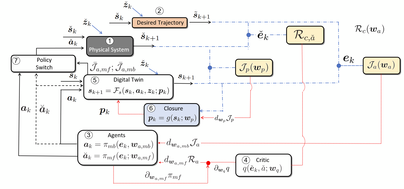
The real system evolves under the influence of control actions , provided by an agent, and exogenous (uncontrollable) inputs . We assume that these consist of a ‘large’ scale () and a ‘small scale’ () contribution, but neither of the two can be forecasted. These are treated as random processes with different integral time scales. With no loss of generality, we assume that observations and actions occur simultaneously. Therefore, in the reinforcement learning terminology, the collection of observations/action pairs within the observation time defines an episode.
The actions seek to keep the system along a desired trajectory (component 2) and we introduce the real error to measure the discrepancy between the current and the target states. The control agent (component 3) acts according to a policy which takes the form of a parametric function in the weights . The control problem involves identifying the weights through an iterative “learning process” while the agent interacts with the system. This process is carried out by evolving two policies in parallel: the best one is promoted to “live” policy and interacts with the real system while the other becomes “idle” and continues to be trained in the background.
One of these policies evolves according to model-free strategy. It is denoted as and is defined by the set of parameters . The other evolves according to a model-based strategy. It is denoted as and is defined by the set of parameters . The decision of which of these becomes “live” or “idle ” is taken by policy switch (element 7 in Figure 1) that selects either or depending on which of the two is producing the best results on the virtual environment and the digital twin (component 5).
The working principle of this policy switch is described in section 4.3. What follows is a description of the model-free and the model-based training, treated as independent strategies.
-
•
The model-free policy () training relies on classic model-free reinforcement learning. The optimal weights are defined according to a reward function, which measures how well the system is kept close to the desired trajectory. This evaluation is made online, updating the policy after each episode. The optimal weights maximize this function, which is written as the summation of instantaneous rewards , discounted by a factor :
(1) The definition of the instantaneous reward function is problem-dependent and discussed in the following sections. As described in section 4.1, the model-free loop implemented in this work is an actor-critic algorithm, which relies on a parametric approximation of the state-action value function in the parameters . This estimates the expected reward for an action-state pair and is essential in computing the update of the policy parameters . This parametric function is referred to as ‘critic’ (component 4) and is essential in computing the gradient driving the training of the agent from the model-free side (see connections in dashed red in Figure 1). We highlight that the use of the error state rather than the state in the reward and functions is here justified by our focus on tracking problems.
-
•
The model-based policy () optimization loop combines system identification and optimal control. System identification seeks to continuously adapt and improve the digital twin (component 5). This is a model of the system which evolves the ‘virtual states’ to , subject to the same exogenous inputs as the physical system and under the ‘virtual actions’ . This solver advances the digital twin in real time and restarts at the end of each episode.
The model relies on unknown parameters , provided by a closure parametric function (component 6) in the weights . This closure function embeds unknown physics or terms that would render the prediction overly expensive. As we shall see in Section 5, these parameters can be classic empirical coefficients (e.g. aerodynamic coefficients or heat/mass transfer coefficients) of a carefully crafted physics-based model of the system. The forward step of the system is driven by an ODE solver, which defines the function .
The system identification consists in finding the optimal weights according to a cost function which measures how close the virtual trajectory resembles the real one. The optimal weights minimize this function, defined as
(2) with the Lagrangian function for the identification problem and the expectation over possible virtual trajectories accounting for the stochastic exogenous inputs. More specifically, starting from one sample signal , with , we build a set of realizations of exogenous inputs as described in section 4.2 and we denote as the set of trajectories generated for a given sample of the exogenous input and a given set of weights . Two reasons motivate the choice for the integral formulation in (2) even if only a discrete set of samples is available. First, the integral is particularly handy in deriving the adjoint problem driving the computation of the gradient , as presented in section 4.2. Second, the choice keeps the approach independent from the specific numerical solver to advance the virtual states . We return to both points in section 4.3. We here stress that the closure model makes the digital twin predictive only for a given sample of the exogenous disturbance signal and within , i.e. no forecasting is considered.
The model-based control seeks to find the optimal policy to keep the digital twin along the desired trajectory. We introduce the virtual error to measure the distance between the current virtual state and the target state and the virtual actions taken on the digital twin. The performances of the controller are measured by the cost function . For convenience, we define this cost function similarly to the one in (2), i.e.:
(3) with the Lagrangian function for the model-based control problem. The same notation as in (2) applies. The optimal control weights for the model-based approach are those that minimize this function. The process of computing a policy update using the virtual environment (model-based loop) without interacting with the real system is here referred to as offline (policy) planning.
It is worth stressing that the weights minimizing in (3) do not necessarily maximize in (1). These problems will not have the same solution unless the virtual environment closely follows the real one. The way these loops interact in the agent’s training is described in the following section, along with more details on the computation of the gradient driving the identification and the gradient driving the agent’s training from the model-based side (see connections in dashed red in Figure 1).
4 Mathematical Tools and Algorithms
We here detail the building blocks of the proposed approach. Only the general architecture is discussed, leaving customizations to specific environments to Section 5. The model-free paradigm (connection of components 1-2-3-4) is illustrated in section 4.1. This leverages standard Deep Reinforcement Learning (DRL) methodologies. The model-based paradigm (connections of components 1-2-3-5-6) is illustrated in section 4.2. This combines adjoint-based nonlinear system identification and adjoint-based optimal control. The model-free and model-based loops could be used independently, and we first introduce their working principle independently. Then, section 4.3 details how these are connected and presents the proposed algorithm.
4.1 The Model-Free loop: (1)-(2)-(3)-(4)
We consider a classic actor-critic reinforcement learning formalism (Sutton and Barto 2018, Bhatnagar et al. 2009). Although more recent variants exist, we here focus on the classic Deep Deterministic Policy Gradient (DDPG) algorithm proposed by Lillicrap et al. [2019] with the prioritized experience replay strategy by Schaul et al. [2015]. This algorithm was extensively benchmarked by Pino et al. [2023] in flow control problems and offers a good compromise between performance and simplicity.
The DDPG trains two ANNs while interacting with the system. The first, referred to as actor, aims to approximate the policy function , which provides the action to be taken at a certain state. This policy is deterministic, but we add noise generated by a random process to explore action space.
The second, referred to as critic, aims to approximate the state action value function ; this provides the expected reward for taking action while the system is in the error state and then following a certain policy. We use to denote the (unknown) true Q value and to denote the approximation from the network. Referring to the previous section and Figure 1, the parameters denote the weights and biases of the actor-network while denotes the weights and biases for the critic network.
These are identified through an online optimization process, which is based on stochastic, momentum-accelerated gradient-based optimization as in classic deep learning (see Goodfellow et al. [2016]). The gradient driving the optimization of the policy reads (see Silver et al. [2014]).
| (4) |
where is the reward function in (1).
The expectation is evaluated on an ensemble of trajectories or transitions and is readily available using back-propagation on the actor and the critic networks. Its accuracy strongly relies on the accuracy of the critic network. The recursive nature of the state value action function allows for measuring the performances of the critic from the Bellman equation [Sutton and Barto, 2018]. For the true Q function this reads:
| (5) |
where . The expectation over possible future states accounts for the stochastic nature of the exogenous inputs, and denote actions according to the current policy (i.e. ). The same recursive form should then exist for the q network. Therefore, defining
| (6) |
the expected state-action value at step , and as the Temporal Difference (TD) error, a cost function for training the critic network can be written as
| (7) |
where the expectation is computed over a set of transitions from one state to the following (regardless of their position in the system trajectory).
The gradient of (7) with respect to can be easily computed using back-propagation on the critic network. However, the training of the critic network is notoriously unstable [Mnih et al., 2013b, 2015]. The two classic approaches to stabilize the learning consist in (1) using an under-relaxation in the update of the weights and (2) keeping track of a large number of transitions by using a replay buffer. The use of both methods is discussed in Section 4.3.
Finally, the sampling from the buffer is carried out in the form of batches to evaluate the gradient . The sampling prioritizes transitions with the largest TD-error, , [Schaul et al., 2016] building a non-zero probability distribution for each sample proportional to it , yielding to the sampling probability of the th transition, equal to:
| (8) |
in which sets the prioritization influence, with implying uniform sampling.
4.2 The Model-Based Loop (1)- (2)- (3)-(5)-(6)
The assimilation and model-based control problem in the loop (1)-(2)-(3)-(5)-(6) share the same mathematical framework. The dynamical system describing the evolution of the digital twin is written as
| (9) |
where is the flow map of the dynamical system and is here assumed to be known.
This function could be derived from first principles, as described in section 5 for the selected test cases, or using a general-purpose function approximator such as ANNs. The distinction is irrelevant to the method presented in this section, and we note in passing that using an ANN to approximate in combination with the training techniques described in this section leads to neural ODEs [Chen et al., 2018].
The problem of training the agent and the closure law is finding the optimal parameters and , respectively, using continuously provided data. The training data consists of a target trajectory for the control problem and measurements of the states for the identification problem. The performances of the assimilating agent are measured according to (2) and (3), respectively (see Figure 1).
These functions are interconnected because they depend on the states, which depend on both the closure variables and the actions (thus both on and ). However, we here consider these independently: should be identified to minimize regardless of the performance of the controlling agent, and should be identified to minimize regardless of the performances of the assimilating agent. This is why only the relevant functional dependency is considered in equations (2) and (3).
To maximize the sample-efficiency training strategy, the optimization of these functions is carried out using gradient-based optimization along with efficient computation of the gradients and using the adjoint method [Errico, 1997, Bradley, 2019, Cao et al., 2003]. This method bypasses the need for computing the sensitivities and . Moreover, because of the similarity in the cost functions (2) and (3), the adjoint problems share key terms. Concerning the gradient driving the system identification, the adjoint-based evaluation gives
| (10) |
where the expectation operator is the same used for the cost function definition in (3), the gradient is readily available from the closure definition and is the vector of Lagrange multipliers (co-states) computed from the terminal value problem:
| (11) |
Similarly, the computation of the gradient driving the training of the controlling agent is:
| (12) |
where the gradient is available from the policy definition (e.g. via backpropagation if this is an ANN) and the evolution of the Lagrange multiplier is determined by the terminal problem:
| (13) |
In both problems, one has one adjoint state evolution and for each of the trajectories used to evaluate the expectation in (10). The methodology to compute the population of trajectories is described in the remainder of this section.
Given a sample of the temporal evolution of the exogenous inputs , with , we build an analytic approximation of its large-scale component using support vector regression [Smola and Schölkopf, 2004]. Let denote the j-th component of the exogenous input sampled at time step . We seek to derive a continuous function such that . This is a regression problem that we tackle with support vector regression. Hence, the continuous function is written as
| (14) |
with , a Gaussian kernel and a user defined scale parameter. We stress that since no forecasting attempt is made. The vector of coefficients is computed by minimizing the cost function (see Chang and Lin 2011)
| (15) |
subject to , and for all in . The coefficients and are user-defined parameters controlling the regularization of the regression.
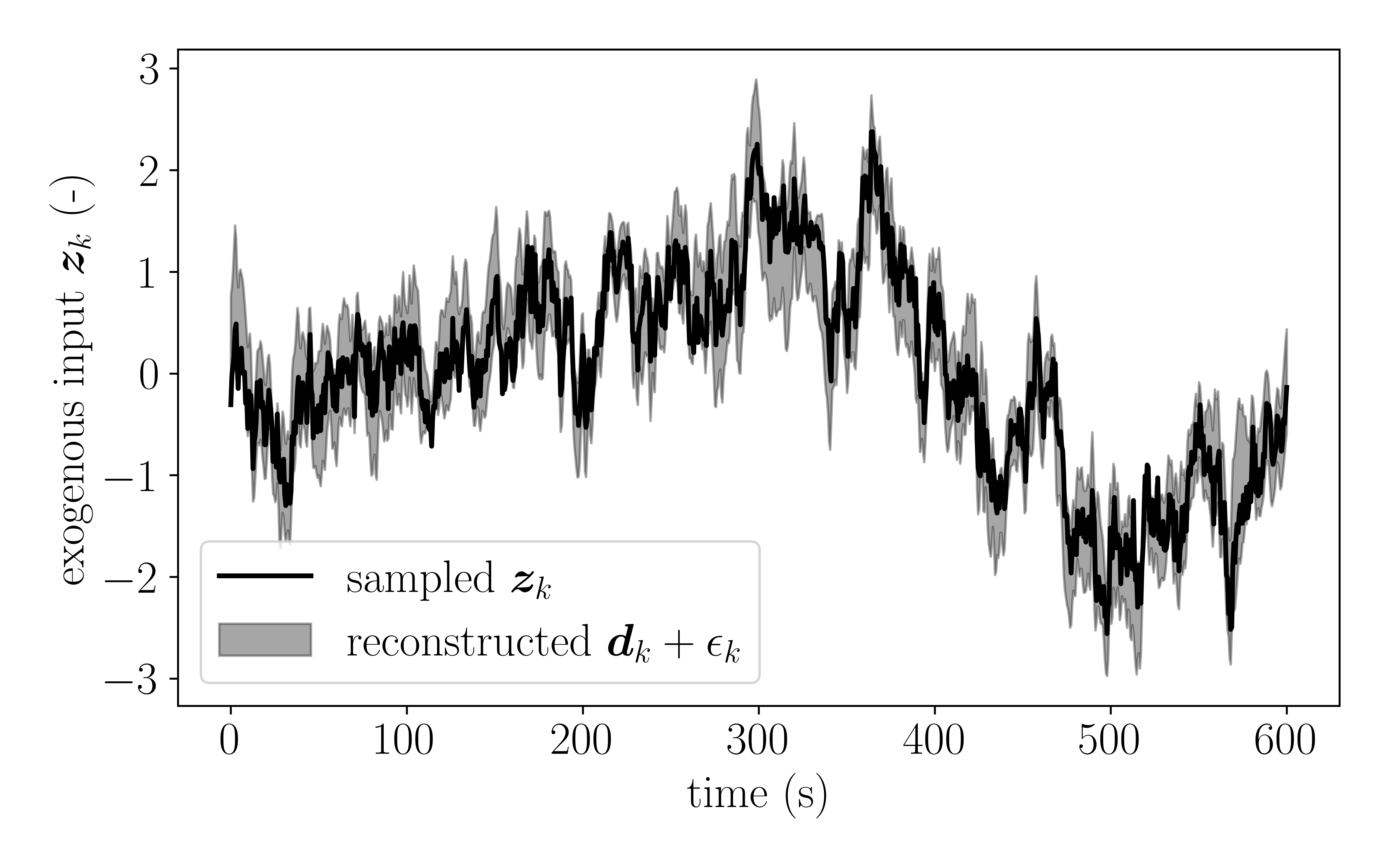
The regression model generates samples of possible exogenous disturbances. These are modelled as a set of Gaussian processes with mean and covariance matrices . We sample these processes times to obtain the exogenous disturbances in the virtual trajectories. This procedure is shown in Fig. 2, for a simulated exogenous disturbance with .
4.3 The proposed RT algorithm
The proposed algorithm is illustrated in 1. It consists of six steps, repeated over episodes. These are described in the following.
-
•
Step 1: Interaction with the real environment (lines 7-13). A sequence of interactions with the real system takes place within an observation time . These episodes are denoted as real as opposed to the virtual ones carried out on the digital twin. These interactions may have an exploratory phase, carried out by adding a random component () sampled from a random process. We here use a Gaussian process with mean and covariance matrix (line 6). The balance between exploration and exploitation is controlled by the sequence , which tends to zero as exploration ends. This sequence could be linked to the performance of the digital twin assimilation, but we leave it as a user-defined sequence for the purposes of this work. During this phase, transitions are stored in the long-term memory buffer and the short-term memory buffer . The first is used to update the critic network and the model-free policy and contains transitions ranked by their TD error (see eq. 7), which is updated as the training of the critic progresses. The second is used for training the digital twin and contains transitions ordered in time and arranged in trajectories. Therefore, contains (random) transitions while collects trajectories. The TD error defines both the sampling and the cleaning of the buffer. The triangular distribution in (8) is used both for sampling and cleaning: the transitions with the lowest probability of being sampled are also the ones continuously replaced by the new ones. On the other hand, no specific criteria are considered for the sampling/cleaning of the buffer , which are simply sampled and stored in chronological order.
-
•
Step 2: Critic Update and model-free policy update (lines 14-24). An optimization with iterations is carried out on the critic network, followed by an optimization with iterations for the policy. Both use batches of transitions sampled from . Concerning the training of the critic network (lines 14-19), this loss function and its gradient are computed from (7). This step is essentially a training of the critic network in a supervised learning formalism. Similarly to what was proposed by Lillicrap et al. [2019] for the original DDPG, the update of the critic is modulated by an under-relaxation using a target network (line 17). At every iteration, the optimized critic re-evaluates the TD errors of the sampled transitions in (line 18). Limiting the TD updates for the current batch of trajectories allows for a pseudo-random update of the most critical transitions, according to the critic. In addition, this approach is also computationally cheaper than re-evaluating all the stored transitions in the buffer, usually in the order of magnitude of . Successively, the critic is then used to train the policy in lines 20-24. In this second stage, the gradient with respect to the cost function is computed using eq (4). Note that we use the notation to denote the optimization update for the weights , such that the updating reads . Therefore, the update in a simple gradient descent over a cost function , for example, reads . This makes the notation independent of the choice of the optimizer. We note that differently from the original DDPG algorithm in Lillicrap et al. [2019], the updates of the critic and the policy networks are carried out via two separate loops rather than in a single one. In our experiments, we found this approach to lead to more stable model-free policy updates.
-
•
Step 3: Fit random processes for exogenous inputs (line 26). In principle, both the forward and backward integration of the ODEs driving the digital twin could be carried out using time steps that differ from the ones controlling the interactions with the real system. This would require some interpolation on the exogenous disturbances as well as on the states and the actions. The data storage between forward/backward evaluations could leverage modern checkpointing techniques (see Zhang and Constantinescu 2023). However, keeping the focus on the first proof of concept of the reinforcement twinning idea, we here assume that the numerical integration (both forward and backward) is carried out using the same time stepping from the interaction with the environment (step 1).
Nevertheless, we use the SVR regression on the exogenous input (see 14) to construct the set of random processes (here treated as Gaussian processes) from which the ensemble of possible realizations of the (stochastic) exogenous input will be sampled. These are used for ensemble averaging of the gradient over possible trajectories. For each of the trajectory available in the short-term memory buffer , we denote as a sample of the Gaussian processes generating the evolution of possible exogenous inputs.
-
•
Step 4: Optimize digital twin on the real actions (lines 27-36). The goal of this step is to find the closure parameters such that the digital twin’s prediction matches with the trajectories of the real system, stored in . Consequently, the loss function in (2) is minimized using a gradient-based optimization loop. This consists of iterations and computes the updates from the gradient evaluated along the trajectories available in . Again, fixing the numerical time stepping to the one of the real interaction avoids the need for action interpolation, but might become problematic for stiff problems. For each trajectory (loop in lines 27-33), a total of possible realizations of the exogenous input are considered (sampled from the processes from the previous step), and the gradient is computed using the adjoint method (see eq. 10). The associated updates are then averaged (line 32), and the optimization step is carried out (line 34). Each optimization step requires a total of forward and backward virtual episodes.
-
•
Step 5: Model-based policy update. (lines 37-43). This step is structurally similar to the previous: it computes the ensemble-averaged adjoint-based gradient (line 41) of a cost function () and performs a number () of gradient-based optimization steps (line 43). In this case, however, the interactions with the digital twin follow the model-based policy instead of the actions stored in . This allows to evaluate the current set of model-based policy weights . The response of the digital twin is governed by the closure law defined by the current best set of weights, i.e. .
-
•
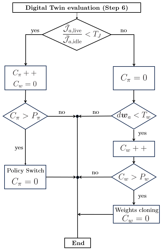
Step 6: Policy switching and parametrization cloning. (lines 44-47). This step decides which of the policies or becomes “live” and which one becomes “idle”. The first is deployed in the next interaction with the real system, while the second continues to be trained with different mechanisms. The decision in this step is based on the policy performances in the virtual environment, evaluated and averaged over episodes with randomized initial conditions and disturbances. Defining as and the averaged cost functions for the “live” and “idle” policies, we introduce a tolerance factor , a threshold , and a counter to avoid overly impulsive decisions. If the live policy performs worse than the idle one more than the tolerance factor (), the counter gets incremented. If exceeds the threshold , the idle policy takes over and becomes the live one. On the other hand, if the opposite is true, then we check that the idle policy did not happen to be stuck in a local minima, analyzing its weight variation:
(16) where indicates the current number of the episode (). To this end, we introduce a tolerance , a counter and a threshold and repeat the previous decision process: if falls below , increases. If goes beyond , it is reasonable to assume that the policy optimization step is trapped in a local minimum, and we replace the “idle” parametrization by cloning the “live” one. The decision tree of this step is recalled in Figure 3.
We close with a few general remarks on the algorithms.
Remark 1
In Steps 4 and 5, the hyperparameters define how much the digital twin should consider past experiences. In this work, we set =1, thus focusing on the last trajectory solely, while having a variable to promote robustness against randomness on the exogenous inputs and take into account possible sampling errors which may occur in real-world scenarios.
Remark 2
The idle policy continues its training through different mechanisms. No special considerations are needed if the idle policy is the model-based policy: this continues to be trained on the digital twin regardless of whether it is active on the real system or not. On the other hand, if the idle policy is model-free, the learning occurs indirectly through two mechanisms that establish a “demonstration” from the model-based to the model-free: (1) the storage of transitions in the memory buffer and (2) the continuous training of the value function Q. The off-policy nature of the reinforcement learning algorithm here implemented allows the agent to learn from policies that are exploratory or simply not ”optimal”, according to the current Q function. In this case, when the model-free policy is idle, and the Q function continues to be updated by observing the model-based policy in action on the real system, a sort of “demonstration” mechanism is established. The fact that the model-free could learn by the demonstration and eventually overtake the lead as a live policy is arguably the most significant contribution of this work.
Remark 3
The model-free update (Step 2), the model-based update (Steps 3,4,5), and the individual evaluations occurring in (Step 6) are independent processes and can be parallelized, greatly reducing computational time.
5 Selected Test Cases
We present the three selected test cases: (1) the control of a wind turbine subject to time-varying wind speed (Section 5.1), (2) the trajectory control of flapping-wing micro air vehicles (FWMAVs) subject to wind gusts (Section 5.2) and (3) the mitigation of thermal loads in the management of cryogenic storage tanks (Section 5.3). These are very simplified versions of the real problems, and the reader is referred to the specialized literature for more details.
5.1 Wind Turbine Control
Test case description and control problem
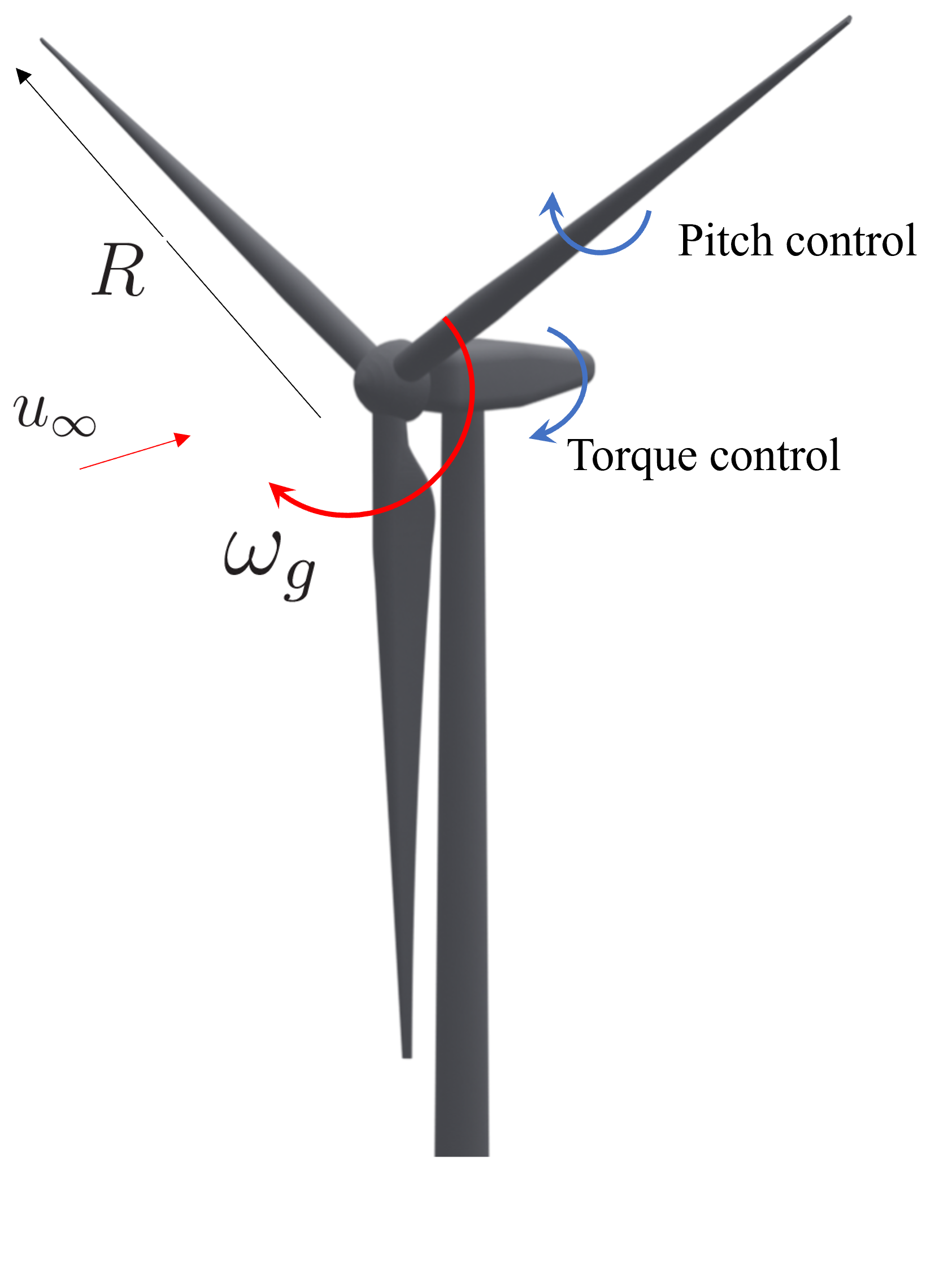
We consider the problem of regulating the rotor’s angular speed and the extracted power of a variable speed variable pitch horizontal turbine of radius , subject to time-varying wind velocity (see Laks et al. 2009, Pao and Johnson 2009).
The operation (and thus the control objectives) of a wind turbine depends on the wind speed in relation to three regions, identified by three velocities: cut-in (), rated () and cut-out () wind speeds. These are shown in Figure 4 for the NREL 5-MW turbine considered in this test case (details in the following subsection). In region 1 (), the wind speed is too low to justify the turbine operation and no power is produced. In region 2 (), the goal is to maximize the energy production. This is usually achieved by pitching the blades at the optimal value and acting on the generator torque to keep the optimal rotational speed. In region 3 (), the turbine is in above-rated conditions, and the goal is to keep the power extraction at its nominal value , thus reducing the aerodynamic load acting on the rotor. This is usually achieved by keeping the nominal generator torque and acting on . Finally, the wind turbine is shut down if , preventing mechanical and electrical overloading.
Particularly critical is the transition between regions 2 and 3 (region 2.5 in Fig.4,) where gusts or lulls could result in shifting of operating conditions, leading to conflicting requirements between torque and pitch controllers. This region is typically handled via set point smoothing, mitigating transients when switching from one control logic to another [Bianchi et al., 2007, Abbas et al., 2020].
In this test case, we combine a Maximum Power Point Tracking (MPPT) controller in below-rated conditions [Bhowmik and Spee, 1999, Howlader et al., 2010] with a regulation control in above-rated conditions. The controller can act on both the generator torque and the pitch angle, receiving as sole input the generator speed , as typically done in multi-megawatt wind turbines [Jonkman et al., 2009]. The current wind speed acts as exogenous input, which we assume can be provided by real-time measurements. We thus collect a sequence with . To avoid high-frequency excitation of the system, we filter the generator speed signal using an exponential smoothing [Zheng and Jin, 2022] with the recursive relations:
| (17) |
with being the low-pass filter coefficient computed as , with the minimum cut-off frequency, the generic raw signal and its low-pass filtered version.
We employ this filter for the generator rotational speed, and the measured wind speed, . From the latter, it is possible to define the target rotational speed and extracted power from the reference curves in Figure 4. In Region 2, these two variables are linked by the operating conditions, while in Region 3, these are defined by mechanical constraints. In below-rated conditions, the power is theoretically maximized if the rotor operates at its optimal tip-speed-ratio . Thus, one can define the reference generator speed relying on the measured wind speed as
| (18) |
where is the gearbox ratio. This variable is constrained in the range , taking into account the machine specifications. Therefore, given the target rotational velocity, we define the tracking errors as , and its integral over the past rotor revolution, , where ensure that both inputs lie in [-1, 1], and consider these as the inputs of the control logic. We then define the actuation vector as
| (19) |
where is a smooth step returning if , if and if . In this work, we define it as
| (20) |
though any differentiable smooth step fits the purposes of bounding the action space while ensuring differentiability. This allows to limit the actuations rate of change according to the actuators’ specifications, and . We further assume that the controller can be informed by measurements of the turbine’s rotational velocity and the generator torque . It is thus possible to define a tracking error on the power as and use this signal to measure the controller’s performance. The reference power follows the -law [Bossanyi, 2000] in under-rated conditions, setting
| (21) |
with
| (22) |
The target power production, also accounting for Region 3, is this . Combining these two references, the cost function driving the model-based optimal control law is
| (23) |
while the for model-free counterpart, we define the reward as
| (24) |
where and ensure that the two components of the cost function have comparable orders of magnitude. The choice of including both the velocity and the power extraction is justified by the fact that these parameters are independent, in the sense that one could extract the same amount of power with different generator velocities by acting on the torque, possibly violating mechanical constraints.
Selected conditions and environment simulator
Disregarding aeroelastic effects on both the blades and the tower, the simplest model of the rotor dynamics is provided by the angular momentum balance, which leads to a first-order system for the turbine’s generator angular speed :
| (25) |
where is the rotor’s moment of inertia, is the aerodynamic torque, is the opposing torque due to the generator and the gear train, and the gearbox ratio. The gearbox efficiency is assumed to be unitary. The aerodynamic torque is linked to the wind velocity as
| (26) |
where is the air density, the turbine’s swept area, and is the power coefficient, that is the ratio between the extracted power and the available one. For a given turbine design, this coefficient is a function of the tip-speed ratio and the blade pitching angle . A predictive model can thus be obtained by combining (25) and (26) and a pre-computed map. This map is usually obtained via Blade Elementum Momentum Theory (BEMT, Moriarty and Hansen 2005), and we do the same for simulating the real environment in this test case. The resulting map for the selected turbine is shown in Figure 5(b).
We consider the NREL 5-MW reference offshore wind turbine [Jonkman et al., 2009]. This turbine has m, kg m2 and rad s-1 for m s-1. The gearbox ratio is . The actuation bounds of the pitch angle and torque actuators are respectively deg and Nm. Their maximum rate of change are deg s-1 and N m s-1, respectively. From these, we define the cut-off frequency as the harmonic associated with the highest rate of change, obtaining Hz and Hz. We set the filter smoothing coefficient according to the slowest pitch actuator, finding .
We take s for the observation time and assume a sampling of Hz for all the simulated instrumentation. We simulate the incoming wind speed time series using the stochastic, turbulent wind simulator TurbSim [Jonkman, 2006] considering a wind velocity with average m s-1 and turbulence intensity TI, thus oscillating between below and above rated. An example of velocity time series is shown in Figure 5(b) together with its filtered signal.
Digital Twin definition
The wind energy community has put significant effort into the development of digital twins of onshore and offshore wind turbines, with applications ranging from load estimations [Pimenta et al., 2020, Branlard et al., 2023] to real-time condition monitoring [Olatunji et al., 2021, Fahim et al., 2022]. In this work, we solely focus on the rotor’s aerodynamic performance and the twinning process seeks to identify a closure law for the power coefficient from data, starting from (25) and (26). In fact, the BEMT, commonly used to obtain the curve, assumes that the flow is steady, and this is questionable in the presence of large fluctuations in the wind speed [Leishman, 2002]. Moreover, the coefficient can change over time as a result of turbine wear (e.g. due to blade erosion) or in the presence of extreme conditions (e.g. ice, dirt or bug buildup) Staffell and Green [2014]. This is why any strategy based on a pre-computed curve is likely sub-optimal [Johnson, 2004, 2006] and the idea of continuous updates of this closure law from operational data has merit. Although this exercise is purely illustrative, the approach can be readily extended to more complex and multi-disciplinary model formulations.
The digital twin employs the power coefficient parametrization formulated by Saint-Drenan et al. [2020]
| (27) |
with the parameters to be identified. This model is known to be valid up to a maximum pitch excursion of deg. Therefore, we limit the maximum allowable pitch command to this value in our experiments.
The assimilation optimizes for , aiming to minimize the error between the predicted dynamics and the real system behaviour . This translates into minimizing the cost function
| (28) |
5.2 Trajectory control of flapping wings micro air vehicles
Test case description and control problem
This test case considers the control of a Flapping-Wing Micro Air Vehicle (FWMAV) which aims to move from one position to another in the shortest possible time. FWMAVs are sometimes considered better alternatives to fixed-wing and rotary-wing micro aerial vehicles because of their higher agility and manoeuvrability [Haider et al., 2020]. The design and control of these drones seek to mimic the remarkable flight performances of hummingbirds, which can undertake complex manoeuvres with an impressive response time (see, for example, Cheng et al. 2016 and Ortega-Jiménez and Dudley 2018).
Reproducing these performances requires advanced knowledge of the flapping wing’s aerodynamics in the low Reynolds number regime, as well as the fluid-structure interaction resulting from the wing’s flexibility. These remain significant challenges for advanced numerical simulations [Fei et al., 2019, Xue et al., 2023]. The proposed test case shows how simplified models of the wing’s aerodynamics could be derived in real-time while an FWAVs seeks to achieve its control target. The considered problem is illustrated in Figure 6(a). A drone initially at m and m/s is requested to move to m as fast as possible, and then hover in that position, i.e. , by continuously adapting its flapping wing motion. We challenge the controller by introducing gusty wind disturbances ,
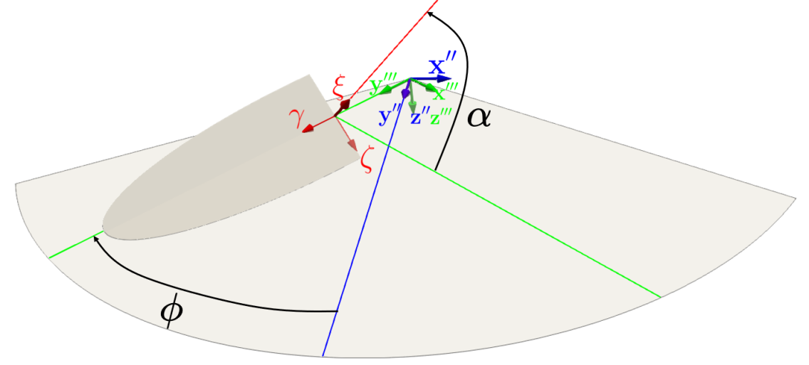
To simplify the body’s kinematics, we consider only 2D trajectories characterized by the position vector defined in the ground frame (). We also attach a moving frame () to the body with no rotational freedom. Starting from the body frame, three Euler angles () and three reference frames characterize the wing kinematics (Figure 6(b)). The wings always flap symmetrically so that the position of one wing defines the other one.
The body frame is first pitched by a stroke plane angle along to define the stroke plane frame (). The wing tips are constrained to flap in the stroke plane () as it flaps along the normal . The flapping frame () follows this rotational motion and defines the flapping angle between the wing symmetry axis and the lateral direction (Figure 6(b)). The last frame is the wing-fixed frame that results from the pitching rotation along the wing symmetry axis. The pitching angle is then defined between the chord-normal direction and the stroke plane axis . The reader is referred to Whitney and Wood [2010] and Cai et al. [2021] for a complete treatment of the flapping wing kinematics. We select an harmonic parametrization for and :
| (29) |
where the beginning of the stroke () is when the flapping amplitude is maximal () and the chord plane is perpendicular to the stroke plane ().
We assume that the flapping frequency and the pitching amplitude are fixed and set the flapping amplitude as a control parameter together with the stroke plane angle , i.e. . We link the action vector to the state error using a Proportional–Derivative (PD) controller with an offset and capped outputs:
| (30) |
where , with , and dots denoting differentiation in time. The control action parameters are and the function is the smoothing operation introduced in (20). The bias terms helps stabilize the drone in hovering conditions once the target position is reached since this operation requires a continuous effort even when the state error is zero.
The reward function driving the model-free controller is written as
| (31) |
where denotes the Hadamard (entry by entry) product and is a vector of two Gaussian functions with mean and standard deviation :
| (32) |
This function is zero far from the target position and unitary once the drone reaches it, so the role of the second term in (31) is to penalize large velocities once the drone approaches the goal. The term in (31) weights the importance of the penalty. The cost function driving the model-based controller reproduces the same approach in a continuous domain and reads:
| (33) |
Selected conditions and environment simulator
We consider a drone with mass g and a constant flapping frequency of Hz. Given the initial position m, we set the target position at m. We assume that the manoeuvre should take less than flapping cycles, hence we consider an observation time of s. This defines the observation time for the twinning. We fix the pitching amplitude to deg and let the flapping amplitude vary in the range (deg). These values are comparable to what is observed in hummingbird’s flight, although the harmonic parameterization in (29) oversimplifies their actual wing dynamics [Kruyt et al., 2014]. The stroke plane angle is bounded in the range (deg).
We assume that the drone’s wings are semi-elliptical and rigid with a span m and a mean chord m. The wing roots are offset of m from the body barycenter, which is also the centre of rotation of the wings. We decouple their motion from the body such that the wing inertia does not influence the body motion [Taha et al., 2012]. This hypothesis simplifies the body dynamics, which becomes only a function of the aerodynamic forces produced by the wings and the gravitational force. These are assumed to apply on the barycenter of the body, which is treated as a material point. Therefore, restricting the dynamics to the plane, the force balance gives
| (34) | ||||
| (35) |
where the subscript refers to forces produced by the wing and the subscript identifies body quantities. Hence the aerodynamic forces produced by the flapping wings are , is the magnitude of the drag force exerted on the body and is the angle between the drag force and the axis. Considering the velocity of the drone and the incoming horizontal wind disturbance (both in the ground frame), this angle is defined as . The magnitude of the drag force is computed as
| (36) |
where is the air density, m2 is the body’s cross-sectional area, is the body’s drag coefficient, here taken as unitary, and is the modulus of the relative velocity between the drone body and the wind, i.e. . The wind disturbance results from a stationary Gaussian process with mean value m/s, in opposite direction to the versor, and covariance matrix defined by a Gaussian kernel with .
To compute the wing forces in (34) and (35) we follow the semi-empirical quasi-steady approach of Lee et al. [2016], based on the work by Dickinson et al. [1999]. This is a common approach in control-oriented investigations (see e.g Cai et al. [2021], Fei et al. [2019]) because it provides a reasonable compromise between accuracy and computational cost, at least for the case of smooth flapping kinematics and near hovering conditions (see Lee et al. [2016]).
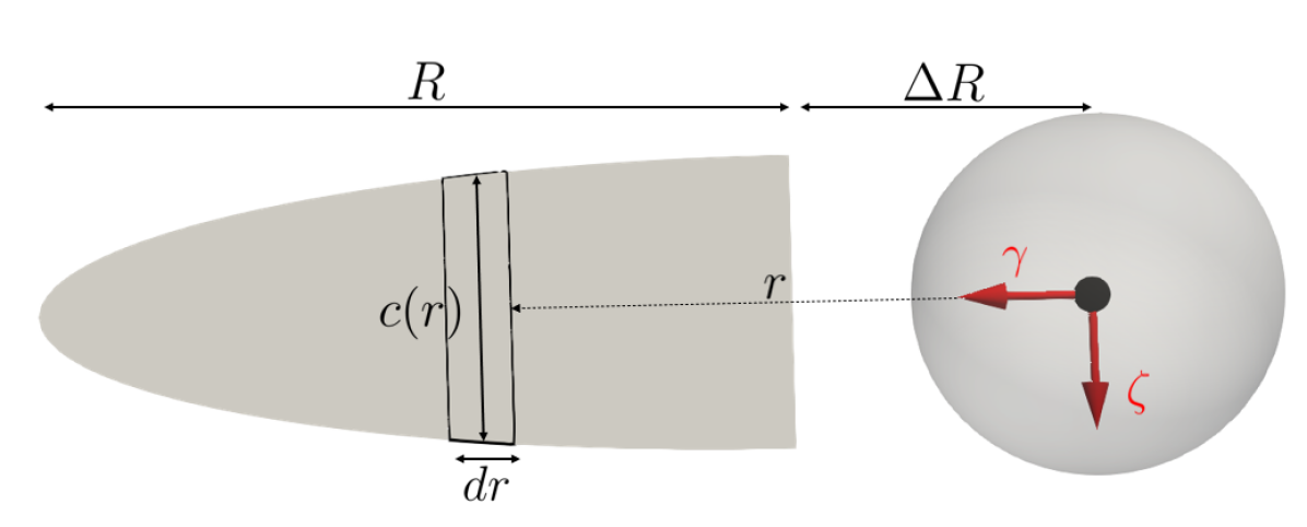
The approach is based on Blade Element Momentum Theory (BEMT), which partitions the wing into infinitesimal elements (see Figure 7(a)). Each element produces an infinitesimal aerodynamic force that must be integrated along the span to get the total lift and drag. In the case of the smooth flapping motion (29), the forces due to the flapping motion dominate all the other physical phenomena (Lee et al. [2016]) so that the lift and drag expressions are
| (37) |
| (38) |
where and are the lift and drag coefficient of the wing and is the modulus of the relative velocity between the wing displacement, the body displacement and the wind. This velocity depends on the span-wise coordinate of the wing section (see Figure 7(b)) and is computed as
| (39) |
The first term is the (linear) flapping velocity of the wing, while the second term gathers the velocity of the body and the wind. Both terms are projected in the wing frame thanks to three rotation matrices:
| (40a) |
| (40b) |
where transform velocities from the frame to the frame, from to and from to .
The force coefficients and in equations 37 and 38 are modeled similarly to Lee et al. [2016] and Sane and Dickinson [2001]:
| (41) | ||||
| (42) |
where are the closure parameters for this problem.
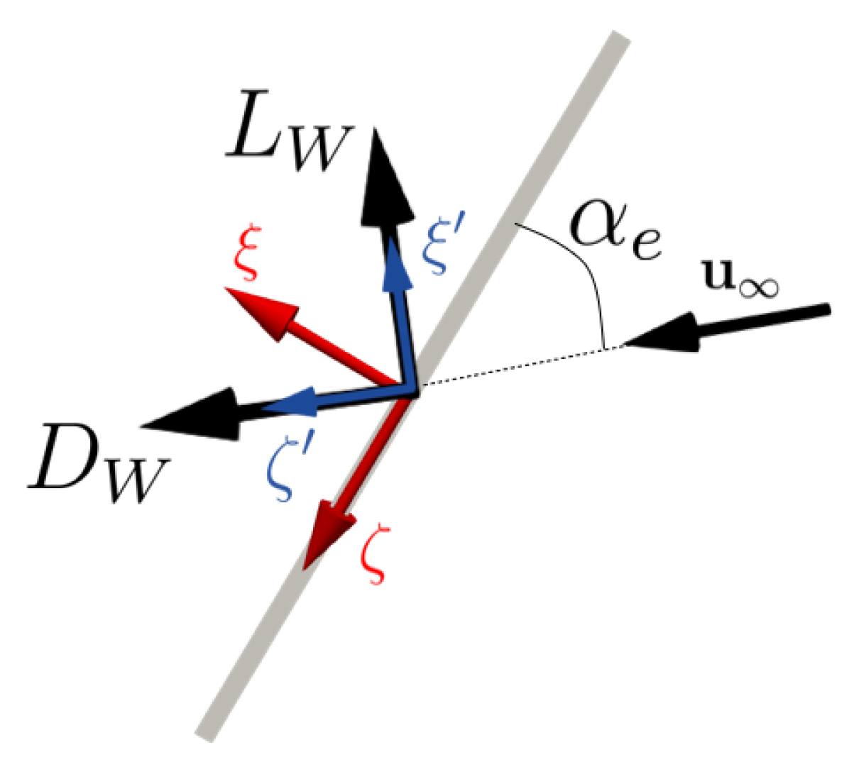
This parametrization approximates the influence of the Leading Edge Vortex (LEV), generated at a high pitching angle due to flow separation and stably attached on the suction side (see Sane [2003]). The corresponding force coefficients depend on the effective angle of attack /, defined between the chord direction and the relative velocity of the wing .
Finally, the forces in equations (37) and (38) were computed in the reference wind frame , which rotates the wing frame by along . The drag is then aligned with while the lift is perpendicular to the drag (Figure 7(b)). These forces are successively transformed into the wing frame and then into the body frame to retrieve and in the dynamic equations (34) and (35).
In this test case, the real environment is simulated using in (37) and (38), as approximated from [Lee et al., 2016] for semi-elliptical wings. For the digital twin, these are the parameters to be identified while interacting with the environment to minimize the cost function:
| (43) |
with the drone position at time .
5.3 Thermal Management of Cryogenic Storage
Test case description and control problem
We consider the thermal management of a cryogenic tank. This is a fundamental challenge in long-duration space missions, which require storing large amounts of cryogenic propellant for long periods. These fluids must be stored in the liquid phase to maximize the volumetric energy density. However, their storage temperatures are extremely low (e.g., -250 ∘C for liquid hydrogen), and their latent heat of evaporation is much smaller than that of non-cryogenic propellants. These combined factors challenge the storage because evaporation due to thermal loads produces a continuous pressure rise over time [Salzman, 1996, Motil et al., 2007, Chai and Wilhite, 2014].
The efficient management of this problem requires a combination of advanced insulation strategies (see Mer et al. 2016b, Jiang et al. 2021) and venting control strategies [Lin et al., 1991]. In this test case, we consider a classic active Thermodynamic Venting System (TVS), similar to the one presented in Lin et al. [1991] and recently characterized in Imai et al. [2020], Qin et al. [2021]. Figure 8(a) shows the schematics of the TVS configuration.
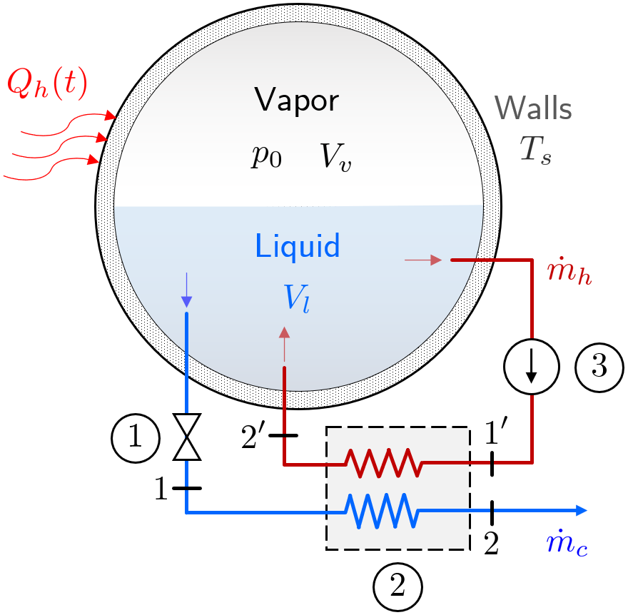
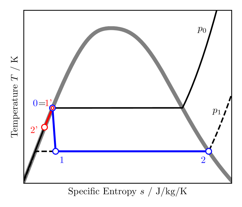
We consider a tank of volume filled with a volume of liquid , operating at a nominal pressure while subject to a time-varying heat load . The TVS is composed of a vented branch and an injection loop. In the vented branch (blue line in Fig.8(a)), a mass flow rate is extracted from the tank, expanded through a Joule-Thomson valve (1) and used as a cold source in a heat exchanger (2) before being expelled. In the injection loop, a mass flow rate is circulated by a pump (3) into the hot side of the heat exchanger and reinjected into the tank as a subcooled liquid. This injection can be carried out via a submerged jet or a spray bar [Hastings et al., 2005, Wang et al., 2017, Hastings et al., 2003], but this distinction is unnecessary for the illustrative purposes of this work. An extensive literature review of TVS approaches is presented by Barsi [2011], who also introduced and tested two simplified approaches for the thermodynamic modelling of the problem (see Barsi and Kassemi 2013a and Barsi and Kassemi 2013b). Figure 8(b) maps the (ideal) key state of the fluids at the inlet and outlet of each component in the (temperature vs. specific entropy) diagram. The state of the liquid and the vapour in the tank are denoted with subscripts () and (), the states () and () are the inlet and outlet of the heat exchanger on the vented line, while states () and () are their counterparts on the injection side.
The control task is to keep the tank pressure below the maximum admissible one while venting the least amount of liquid. The simplest control problem, and also the one implemented in this work, consists of employing the pressure difference as the sole control parameter. The is linked to the mass flow rates in the J-T valve (1) and the pump (3) by limiting the operating range of the heat exchanger and by imposing that only latent heat is to be recovered from the venting line. Therefore, defining as the temperature drop produced by the J-T device and the specific latent heat remaining on the vented line, one has
| (44) |
Furthermore, to limit the control action exclusively to , we assume that the pump (3) is equipped with flow regulation to follow (44) and we link the vented flow rate to and the J-T valve’s characteristic through
| (45) |
with the valve’s pressure drop constant. Considering the maximum pressure drop along the JT-valve , the desired operational pressure and defining the tracking error, we consider a simple policy parametrization of the form
| (46) |
We treat as a pre-defined constant and use as policy parameters. acts as an offset in the policy, controlling the threshold pressure above which the valve opens, while controls the slope of the hyperbolic tangent, i.e. the sensitivity of the policy to the tracking error. The cost function driving the model-based controller and the model-free agent are
| (47) |
with the used to non-dimensionalize the inputs and weight the penalty on the mass consumption versus the primary objective of keeping the pressure constant.
To set up the data-driven identification to this control law, we assume that the tank is instrumented with a pressure sensor sampling and a flow rate sensor on the vented line to measure .
Selected conditions and environment simulator
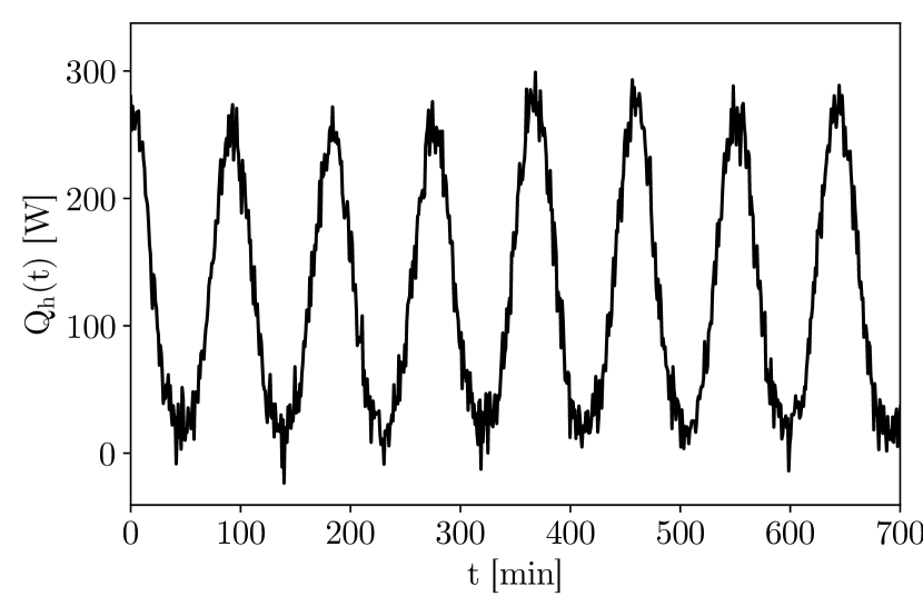
We consider a cryogenic tank with volume m3 with a desired operational pressure kPa filled with liquid hydrogen. At the start of each episode, the tank is full and pressurized to an initial value sampled from a normal distribution with mean kPa and standard deviation kPa. The thermal load applied to the tank fluctuates from a minimum of roughly W to a maximum of W with a period of h. This cyclic load mimics the large thermal fluctuations a tank could face in orbit as it is periodically exposed to direct sun radiation. The chosen period is approximately the time it takes the International Space Station (ISS) to complete an orbit around Earth. The load profile is shown in Figure 9(a). This load is constructed as a pseudo-random signal made of Gaussian-like peaks randomly varying within times the nominal peak, lifted by the minimal load and polluted by uniform noise with a standard deviation equal to the nominal peak.
The simulation of the real environment and the digital twin are carried out using the same simplified model. In particular, we employ the homogeneous model presented in Barsi [2011], adapted to account for the venting line similarly to Mer et al. [2016a]. This approach assumes that the liquid and the vapour are in saturation conditions. This is an oversimplification because usually the liquid is subcooled, and the vapour is superheated. We consider two control volumes: the saturated mixture and the solid wall. We refer to Marques et al. [2023] and Barsi and Kassemi [2013b] for more advanced models and to Panzarella and Kassemi [2003] and Panzarella et al. [2004] for an in-depth discussion on the limits of thermodynamic models. Focusing only on the storage problem (no out-flow except venting), the conservation of internal energy of the solid, and the mass and enthalpy of the saturated mixture read
| (48a) | |||
| (48b) | |||
| (48c) |
where is the density, is the specific enthalpy, and is the variation of specific enthalpy on the injection loop provided by the heat exchanger. All properties are at saturation conditions, and the subscripts and refer to the liquid and the vapour phases, respectively. We consider the mass and specific heat capacity of the wall to be constant. Denoting as the (volumetric) enthalpies and using the chain rule to have , these can be written as
| (49a) | |||
| (49b) | |||
| (49c) |
The heat transferred from the wall to the fluid mixture is modelled using Newton’s cooling law , where is the overall heat transfer coefficient. Taking all liquid and vapour properties from thermophysical property libraries, this is a closed set of implicit differential equations for . The fluid properties are retrieved through the open-source library CoolProp [Lemmon et al., 2018], which is based on multiparameter Helmholtz-energy-explicit-type formulations and also provides accurate derivatives.
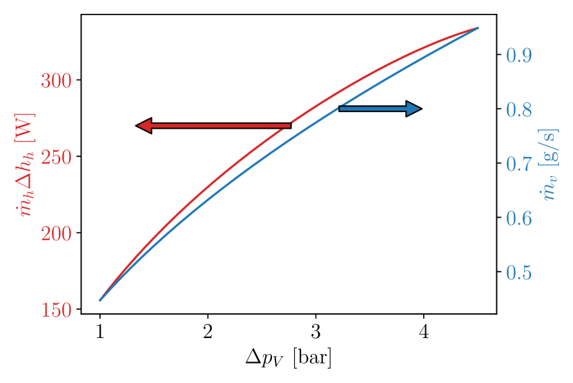
For a given design of the evaporator, one can link the subcooling in the injection line (term in (48c)) to using standard methods for heat exchanger design (see Cengel and Ghajar 2019). This can be written as , with the efficiency of the heat exchanger, the number of transfer units and the overall heat transfer coefficient. For the sake of this problem, we assume that the heat exchanger is a shell-and-tube design with 200 tubes of mm diameter and m length, for a total exchange area of m2. Taking a wall/fluid heat transfer coefficient of W/(m2K), a global heat transfer coefficient of W/(m2K) and a valve with GPaskg2 gives the thermal power exchange and the vented flow rate in Figure 9(b).
Model predictions are thus possible once these three parameters are provided. We consider these the model closure for the digital twin, hence . These are to be inferred from real-time data by minimizing the following cost function.
| (50) |
where the parameters are used to give comparable weight to these terms despite the largely different numerical values. To simplify the calibration of this digital twin model, in addition to the pressure sensor, we assume that a liquid level indicator is available, allowing for monitoring the liquid level , as well as temperature sensors to acquire .
6 Results
This section presents the performances of the RT algorithm in controlling and assimilating a wind turbine subject to time-varying wind speed (T1, 5.1), a flapping wing micro air vehicle (FWMAV) against head wind (T2, 5.2) and a cryogenic tank exposed to fluctuating thermal load (T3, 5.3). The hyper-parameters selected for each test case and the respective simulation configurations are listed in Table 1. We use five different random seeds for our simulations to extract performance statistics across different initial states of the optimizers. For both T1 and T2 we take the gradients ensemble over 5 realizations, whereas in T3 we considered 1, for the overall limited level of noise in the exogenous disturbance. In all studies, the first policy to be deployed onto the real system is the model-free one. Finally, for all test cases, we set 1, as detailed in Section 4.3.
| (s) | dt (s) | |||||||||||
|---|---|---|---|---|---|---|---|---|---|---|---|---|
| T1 (Sec. 5.1) | 600 | 5 | 20 | 5 | 500 | 1000 | 15 | 10 | 2 | 3 | 1 | 0.5 |
| T2 (Sec. 5.2) | 5 | 5.0 | 20 | 5 | 1000 | 1000 | 15 | 5 | 4 | 4 | 1 | 0.5 |
| T3 (Sec. 5.3) | 4.32 | 30 | 20 | 1 | 1000 | 1000 | 30 | 5 | 4 | 20 | 1 | 0.5 |
6.1 Learning Performances
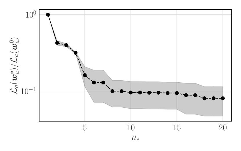
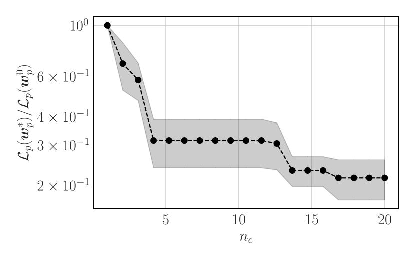
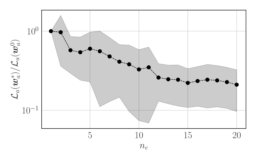
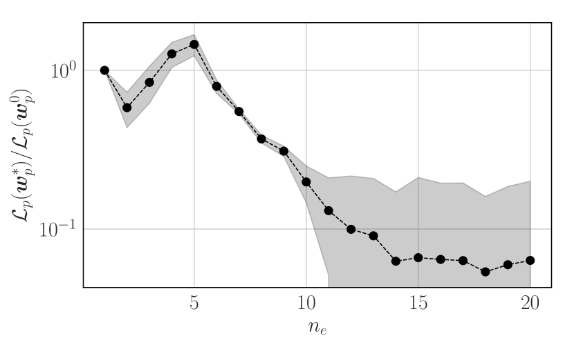
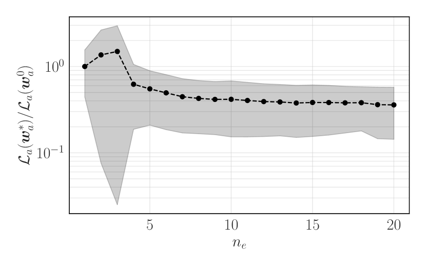
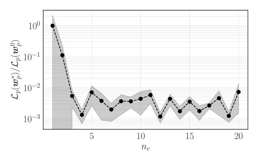
The learning performances for all the three cases are reported in Figure 10 and their numerical values tabulated in Table 2. The Figure shows the mean control or assimilation performances (first or second column, respectively) as a dashed line, and their relative standard deviation as a shaded area. The joined model-based and model-free control paradigm learns how to control effectively the system in a limited number of iterations for all test cases, showing good sample complexity. Indeed, the average control performance () is in the order of with respect to the initial condition, performing thus up to ten times better the initial policy. The high standard deviation at the beginning of the training is associated with the initial exploration phase of the model-free side, and it consistently decreases with the iterations, as it converges to a specific region of the search space, as shown in Figures 10(c) and 10(d) whereas in Figure 10(a) it is roughly constant. Analysing the adjoint-based assimilation performances, Figures 10(b), 10(d) and 10(f) show that the methodology is able to tailor the digital twin on the current system specifics in five to ten iterations. At the end of the training process, it obtains an of , and , normalized with the performances of the initial guesses of , for T1, T2 and T3, respectively. This, in turn, reflects on the model-based policy optimization (Step 5). In fact, as the digital twin predicts with greater precision the dynamics of the system for different actuations also the quality of the policy optimized “offline” increases. This also affects the policy switch (Step 6), as it becomes more accurate in choosing the best policy to be deployed on the real system. The effect of Step 6 is illustrated in Fig. 11.
| T1 (Sec. 5.1) | (2.1 0.8) | (0.8 0.5) | (1.3 1.2) |
|---|---|---|---|
| T2 (Sec. 5.2) | (3.2 4.9) | (4.18 0.01) | (2.01 0.45) |
| T3 (Sec. 5.3) | (3.15 0.9) | (4.47 2.68) | (4.80 3.15) |
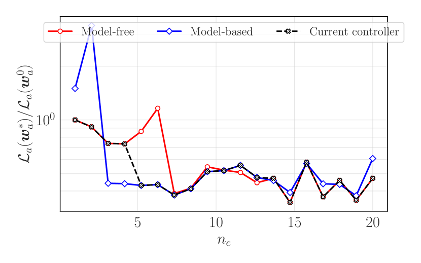
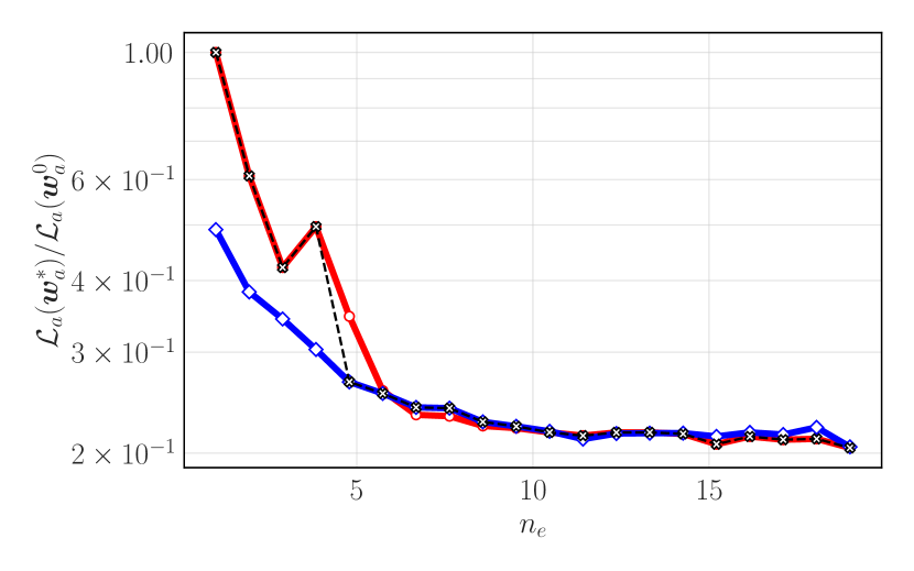
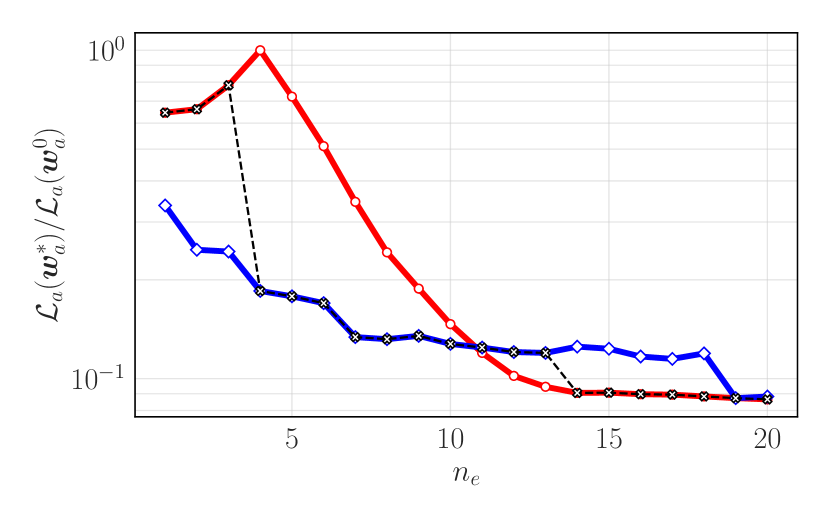
All experiments begin with the model-free policy driving the interactions with the real environment, i.e. as “live policy”, while the model-based is initially set as “idle”. Then, if the model-based performs better for iterations, it takes over as “live” policy following the decision tree of Step 6, illustrated in Figure 3. This is what happens at in T1, and for both T2 and T3. When this happens, the two paradigms, model-based and model-free, start to interact, as shown in Figure 11 especially appreciable in Figures 11(a) and 11(c). We observed that as soon as the model-based takes the lead of the interactions with the real system the model-free control performance registers a steeper improvement. Arguably, this has two causes: (1) the model-based acts as an “expert” for the model-free, providing high quality samples recorded in from which the model-free loop can learn; and (2) the critic gets better at predicting the value associated to the recorded transitions. Interestingly, in both T1 and T3 (Figure 11(a), 11(c)), the model-free learns a better policy imitating the model-based counterpart, effectively “surpassing the master” and being selected to be the “live” policy again. Comparing the performances of the model-based and model-free loops, In T1 the model based performs slightly better, in T2 the model-free performs roughly 50% better than the model-based and in T3 they converge to the same policy, thus we could not conclude about the general performance of the model-based and model-free policy optimization loops.
6.2 Wind turbine Control
The digital twin performances, parametrized by the best set of weights , are shown in Figure 12. Figure 12(a) shows the average prediction versus the average system evolution as a function of time, while Figre 12(b) in the middle plots one versus the other. We conclude that the digital twin successfully tracks the dynamics of the real system. However, it shows a a systematic under-estimation of roughly (rad / s) or 9.55 (RPM), especially localized at low rotational speeds. Whether this bias is inherently linked with the chosen parametrization or an insufficient number of samples requires further investigation. It is worth of notice that, while in T2 and T3 the coefficients to be identified represent the “ground truth”, in this test case there is not such a baseline, as the initial coefficients , derived in the work of Saint-Drenan et al. [2020], describe a power curve in steady wind conditions. As a consequence, the RT algorithm optimizes them to adapt to the dynamic a time-varying wind field as the system progresses. Therefore, the average assimilator loss highlights the capability of the algorithm to adapt online, possibly taking into consideration changes in the operative conditions of the system itself, i.e. blade erosion and relative decrease in aerodynamic performances.
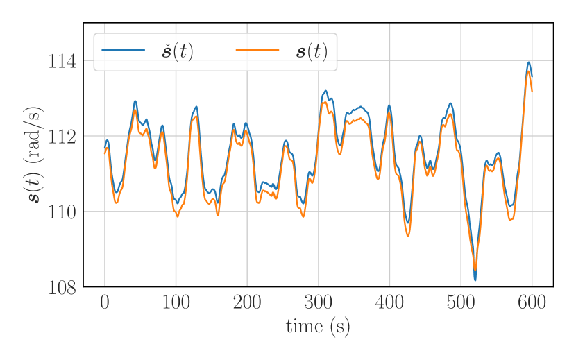
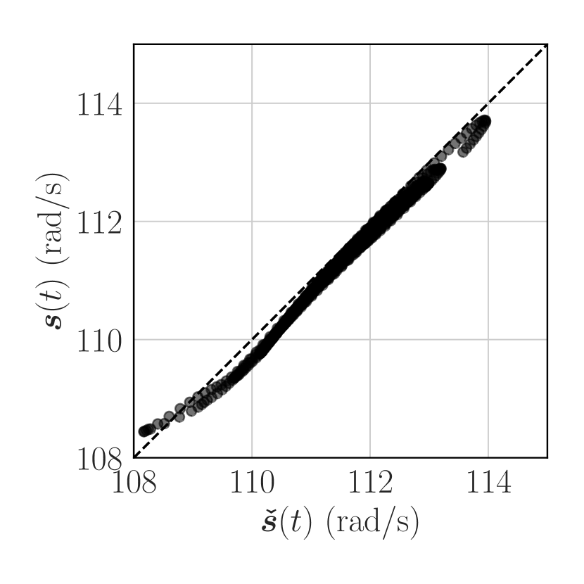
The control performances are summarized in Figure 13. The controller is able to keep the system close to the desired set-points, Figures 13(a) and 13(b). This is especially true for what concerns the power, always kept very close to , even in noticeably varying wind speeds (Figure 13(b)). On the other hand, it consistently keeps the generator speed, , below-rated conditions, of approximately rad/s. This lower-than-rated rotational speed reflects on the actuated torque, Figure 13(d), which is always in the middle between the allowed action space. In addition, the very fast actuation rate on the torque, = 15 kN, allows the controller to rapidly adapt in case of abrupt change in the wind speed, while fine tuning the actuation with the pitch angle, . The latter follows consistently the wind speed, which is desirable. At higher wind speeds than rated, i.e. m/s, it consistently plays on the blades’ angle to reduce the aerodynamic torque to keep the system close to desired conditions. We note that this lower-than-rated strategy be mitigated, if desired, tuning the normalization coefficients and , possibly increasing the penalty commonly done in multi-objective optimization problems.
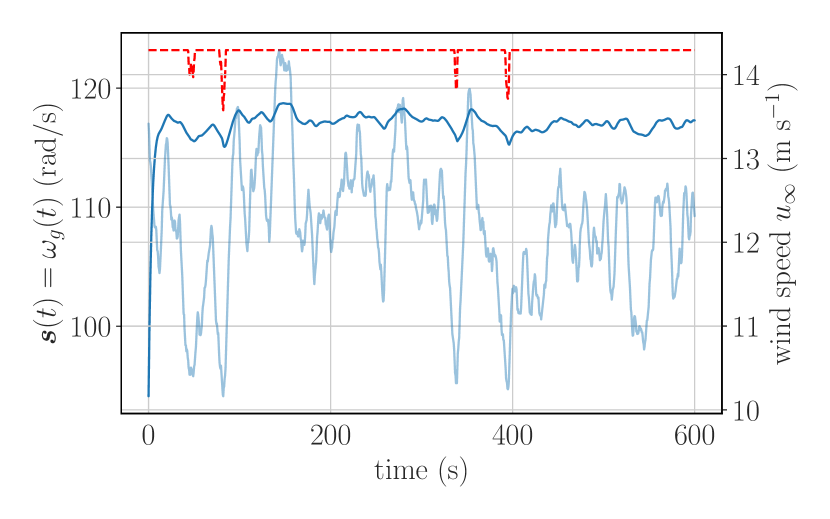
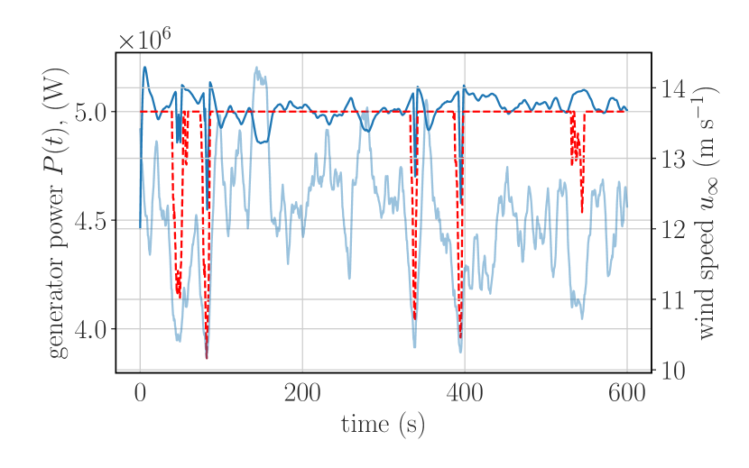
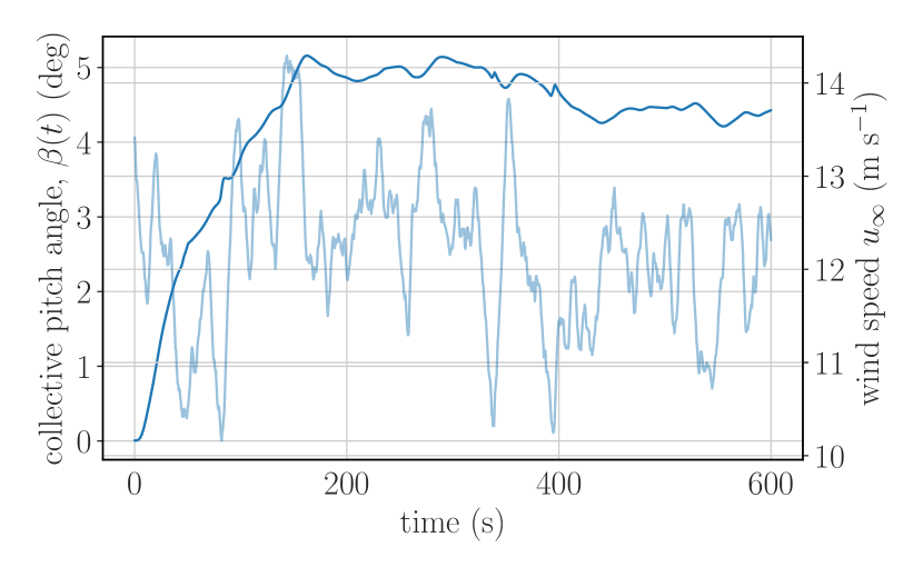
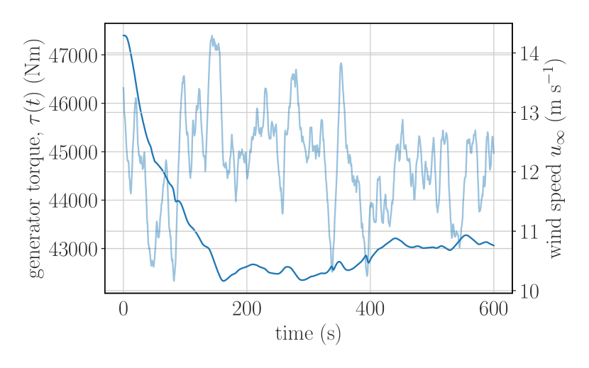
This decrease in is better appreciated in Figure 15(b), which shows the power coefficient trend against wind speed. This shows a peak, at rated conditions (m/s) with a , steadily decreasing for higher winds, as expected in common wind turbine control strategies.
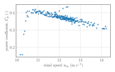
The model-based and model-free policies are compared in Figure 15. The two optimization loops converge to essentially the same parametrizations, leading to the same policy functions, as also supported by the very similar mean cost functional listed in Table 2. The only (minor) difference appearing to be the threshold in the actuation of the torque. In both cases, when the error goes on the rotational speed goes negative, i.e. , the controllers reduce the pitch angle (Figures 15(a),15(c)) to increase the aerodynamic efficiency and, consequently, the harvested aerodynamic torque, with the goal of increase the rotational speed to get closer to the set point. The opposite is true when the generator is spinning too fast: the controller increases the angle of attack of the blades to slow the generator down. The integral of the error over the past revolution, , essentially decides on the slopes of the control surface. Interestingly, looking at the torque actuation shown in Figures 15(b), 15(d), it seems that this control actuation is almost insensitive to this control input, relying on the scalar error solely. This control surface is directly connected with the objective of keeping the power around the rated value of . In fact, as the error becomes negative, the controller increases the torque, to keep the power at the end of the generator constant (). On the other hand, when the error increases, it reduces the resistive torque, relying on the pitch actuator to reduce the speed while keeping the power constant.
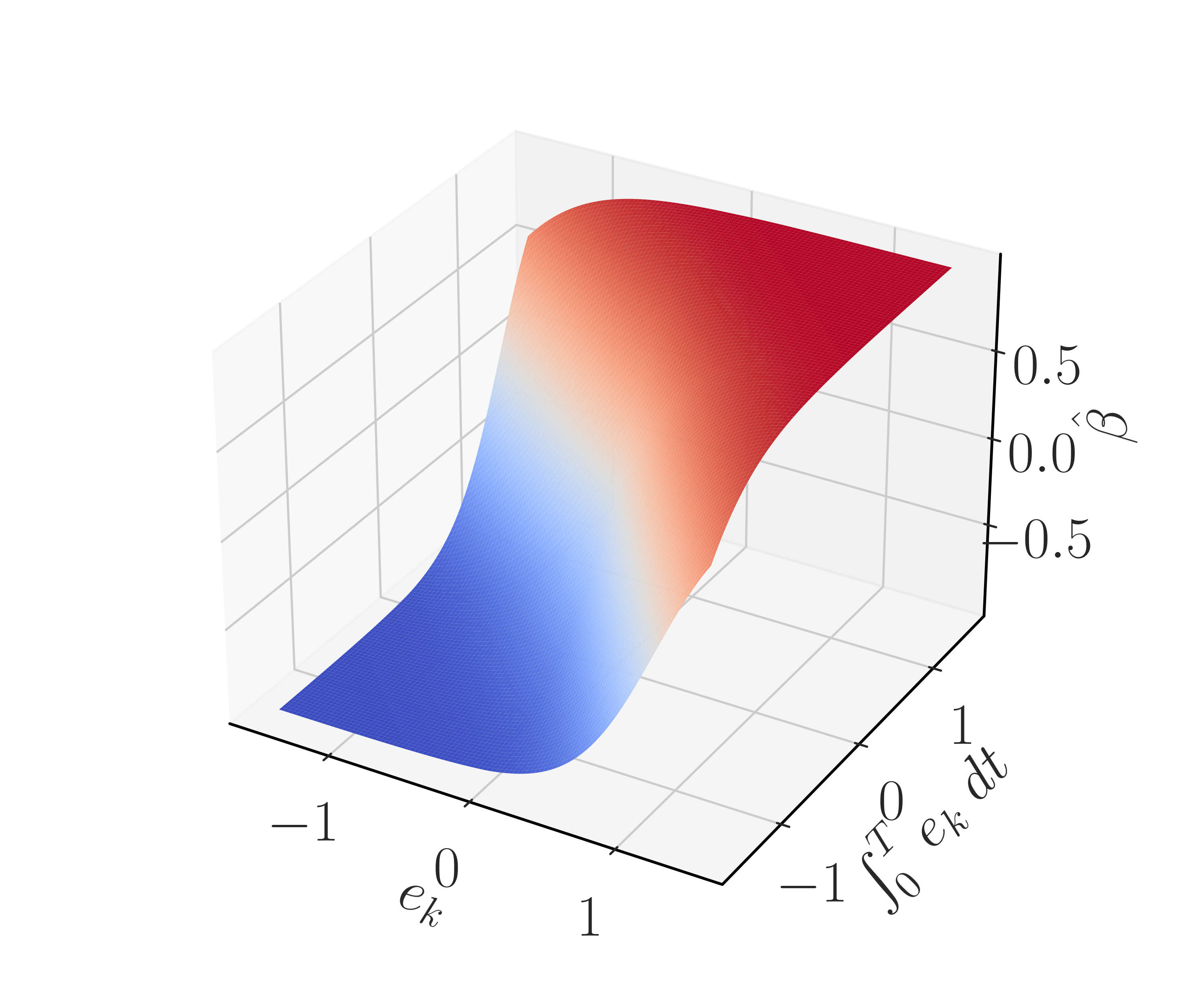


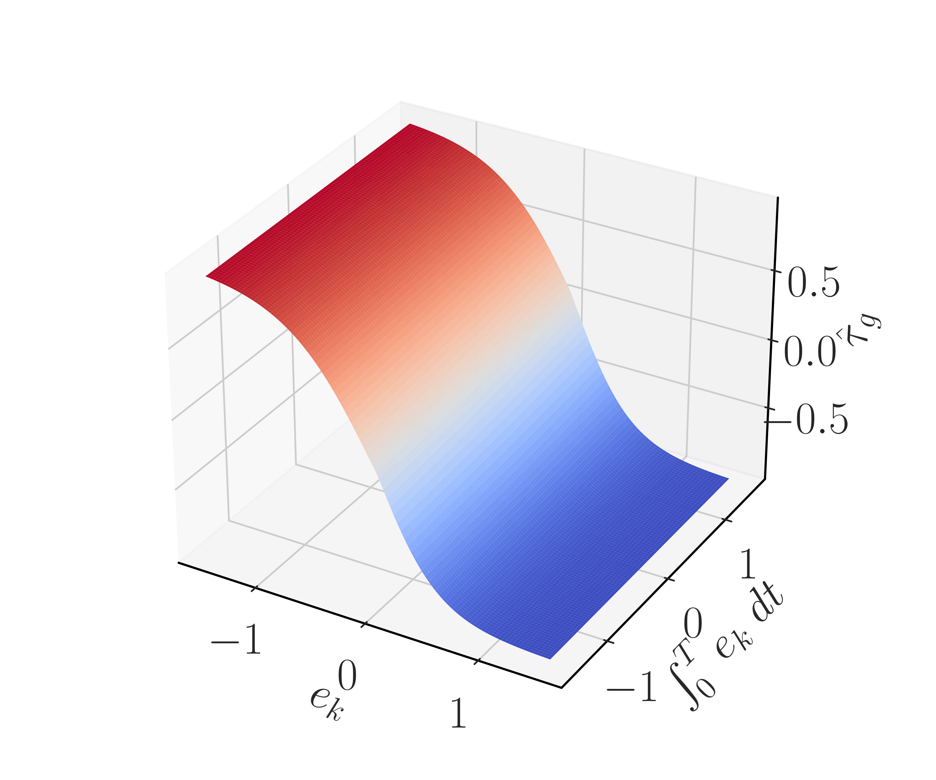
Lastly, we conclude this analysis investigating the robustness of the found models, shown in Figure 16(b). Specifically, we run one-hundred simulations, on randomized initial conditions and sampled disturbances, possibly unseen during the training phase, using the found policies parametrizations , and assimilation parameters . The control performances, Figure 16(a) show a multi-modal distribution. The stronger peak is located in a good performance region, close to . This supports the good performances shown above. However, it appears that the model is not able to extrapolate the control strategies in unseen conditions outside of a given “confidence” region. This may be due to several factors. A first hypothesis is that it could be beneficial to use more wind fields time series (and relative realizations) to get a broader picture of the possible operative conditions, possibly increasing their diversity, or considering an higher number of realizations . Another way of possible improvement may lie in the function approximators used for the policy function, currently just a linear combination of the inputs, which could possibly increase the descriptive capabilities of the model. Nevertheless, we considering the control task successfully achieved for the nominal operative conditions and leave these investigations for future works more centred on wind turbines control. The assimilations performances, on the other hand, are reliably on-track with respect what experienced during the learning phase. The digital twin tracks the real system with very small deviation, for most situations. However, this model may also be improved to take into account both the minor bias presented in Figure 12 and to be more flexible in adapting to new conditions.
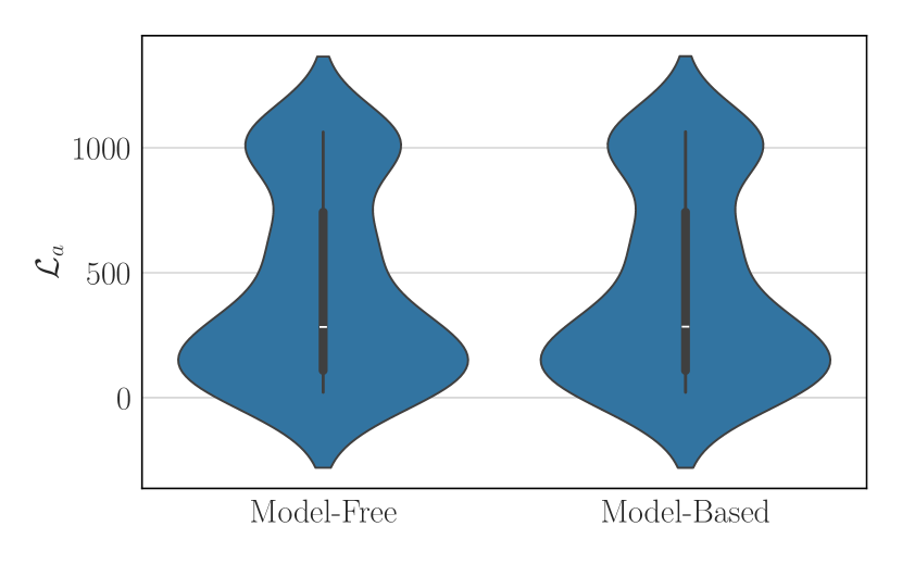
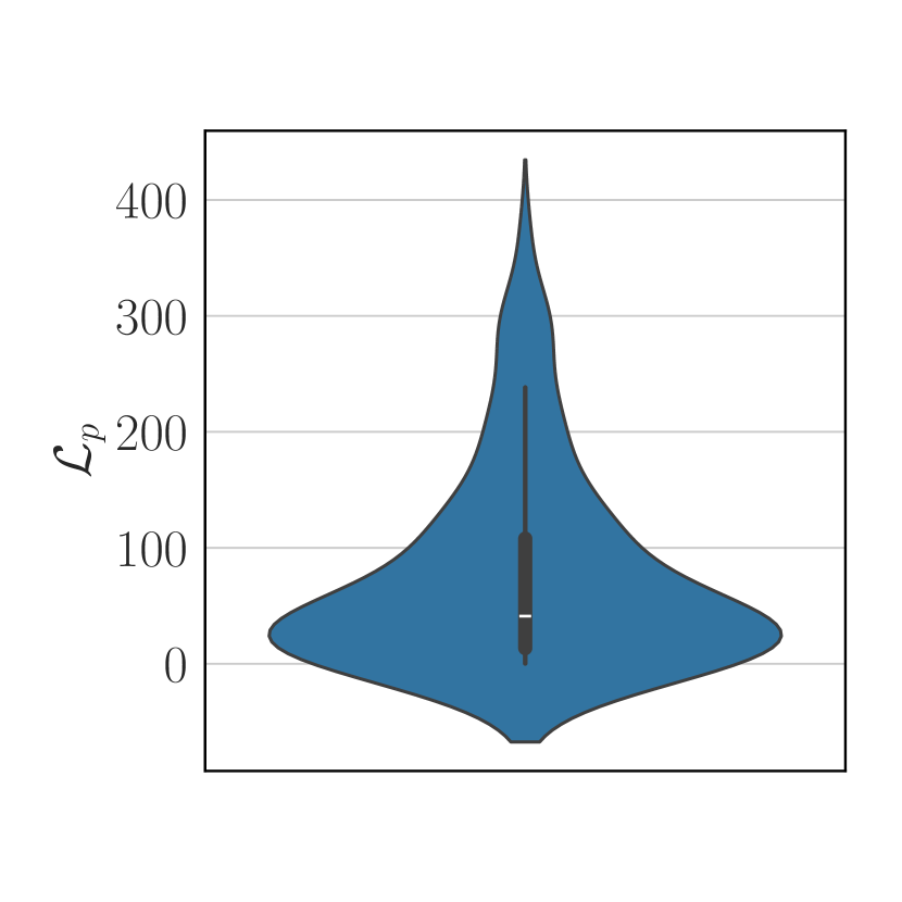
.
6.3 Trajectory control of flapping wings micro air vehicles
In this test case, the initial weights , pertaining the lift and drag closure (equation (41) and (42)), are drawn from three random distributions, and a stopping criterion was defined to interrupt the iterations if the cost falls below a given threshold (). Figure 17(a) shows the assimilation performance of the digital twin in predicting the real-system behavior. The two show a small deviation. This can be better appreciated in Figure 17(b), which shows that the states predicted by the digital twin (y-coordinates) corresponds with good agreement with the true states (x-coordinate) experienced by the real environment, thus lying on the diagonal of the plot.
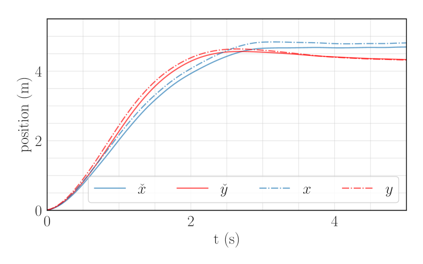
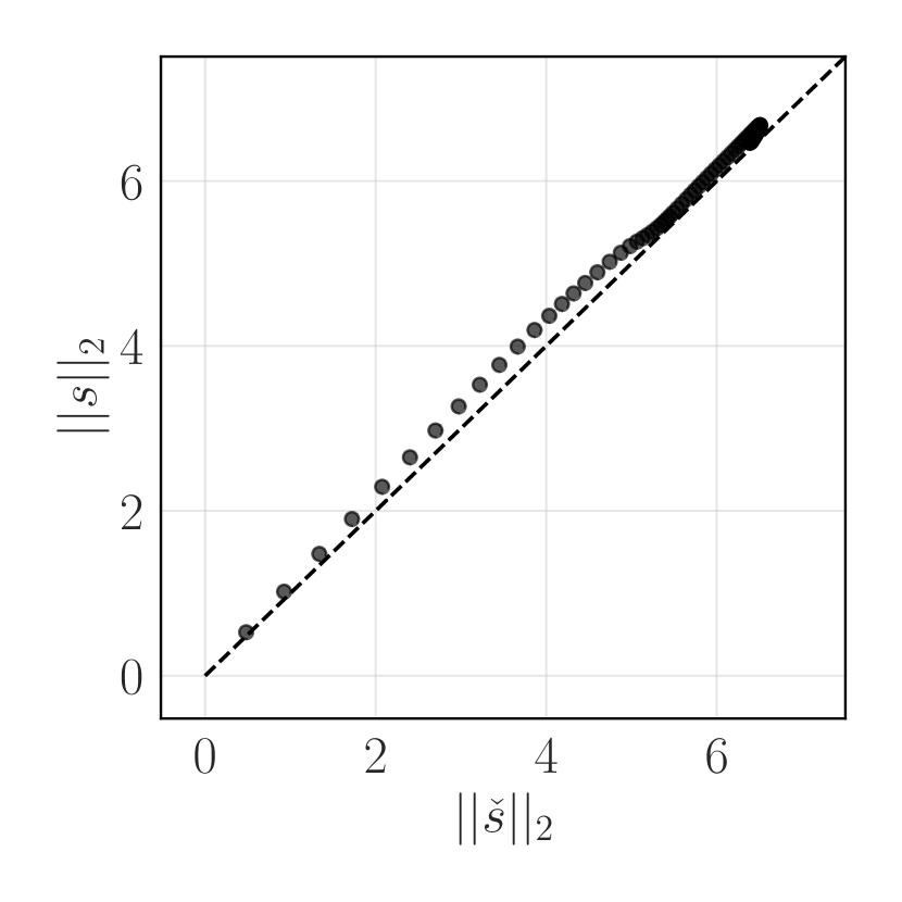
The training detailed in Section 6.1 converges to one optimal policy that the drone applies to control its flight in the real environment. Figure 18 characterizes one such flight depicting the state variables (18(a) and 18(b)) and the control actions (18(c)). The figures evidence that the drone managed to closely reach its target ( m and , as fast as possible) thanks to the control of the stroke plane angle and the flapping amplitude . The control of the latter is mainly formed of three phases in a kind of bang-bang fashion. First, the drone flaps its wings at their maximum angle of attack ( deg) to reach the target position as fast as possible. Then, the drone picks a flapping angle close to the minimal one ( deg) to decelerate and stabilize at the target height with minimal overshoot. Finally, the wings flap at a slightly bigger angle so that they generate enough lift to balance the body weight. The lift is also slightly modulated by the other control variable () which mainly drives the horizontal motion of the drone. At the start of the episode, the drone pitches the stroke plane up to the maximum angle ( deg) and then stabilizes it around an angle that allows it to stay close to the desired position, , despite the headwind. The influence of the gust is visible on even though the wind effect is still very limited, due to the selected mass and surface of the body.
Figure 19 analyses the policies found by the model-free (Figures 19(a) - 19(d)) and model-based (Figures 19(e) - 19(h)) loops. To this end, we fix two of the four inputs to zero and span on the other two dimensions, recording the corresponding action. The two policies are remarkably similar, converging to essentially the same parametrization with their differences lying in the concavity of the hyperbolic tangent, as dictated by the biases. This affects the localization of the switching between the two bounds of the actuation space, possibly explaining the differences in their associated costs presented in Table 2. In both cases, for what concerns , the demarcation zone between the two bounds lies on the diagonal that goes from to , see Figure 19(a). The same trend is observed in Figure 19(b), which analyses the dependencies from and its time derivative. In this case, however, the upper point of the diagonal lies around , thus increasing as the rate of change of goes negative, and decreasing it otherwise. Interestingly, the model-based policy here shows a broader decision zone, as depicted in Figure 10(f). Now, analysing the actuation on , the threshold appears to be positioned in the diagonals to . The sensitivity to the errors instead show it to lie in and . Therefore, it seems that the time variation of the rate of change is the most important input on the dimension, whereas in the coordinate, it is the scalar . Arguably this may be caused by the headwind, oriented as opposite of the versor. Overall, there appears to be two main mechanisms at play: (1) the errors and their rate of change seems to have the same importance when deciding how to control on being slightly more sensitive to the scalar instantaneous errors; and (2) when deciding on how to actuate , the controller balances the scalar instantaneous error in one dimension and its rate of change in the other. In fact, when increases, it actuates on to get back to nominal conditions, and the same is observed on analysing the reactivity to the instantaneous error and .
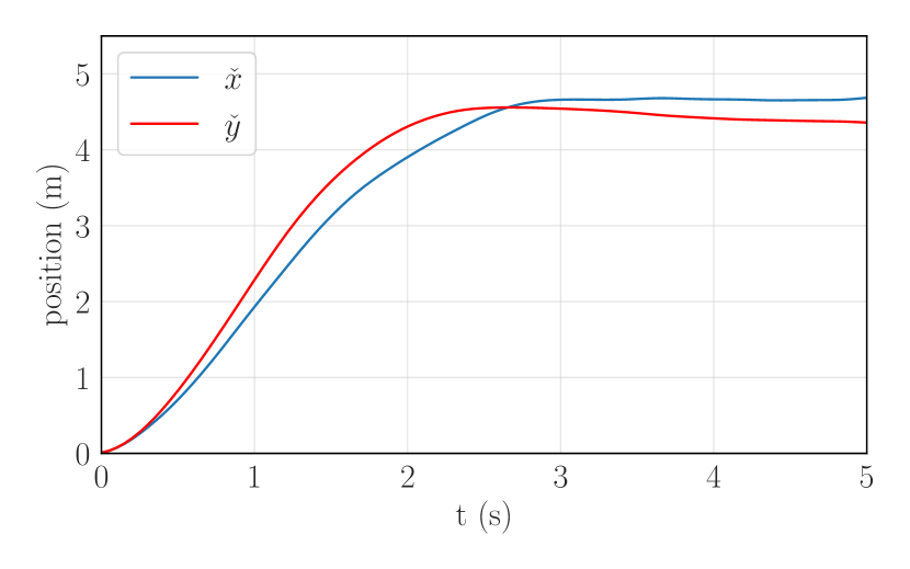
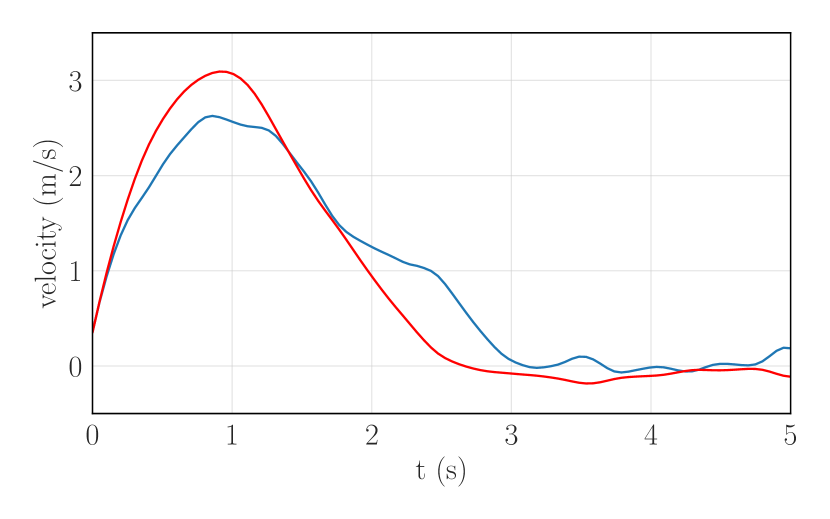
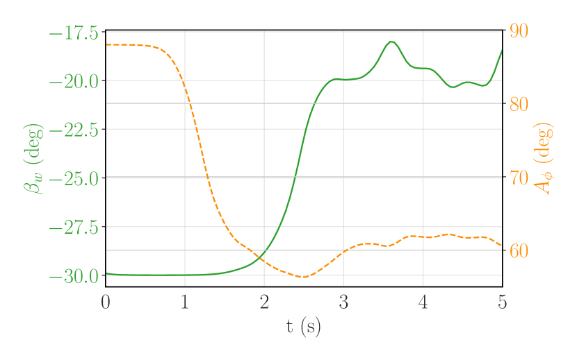
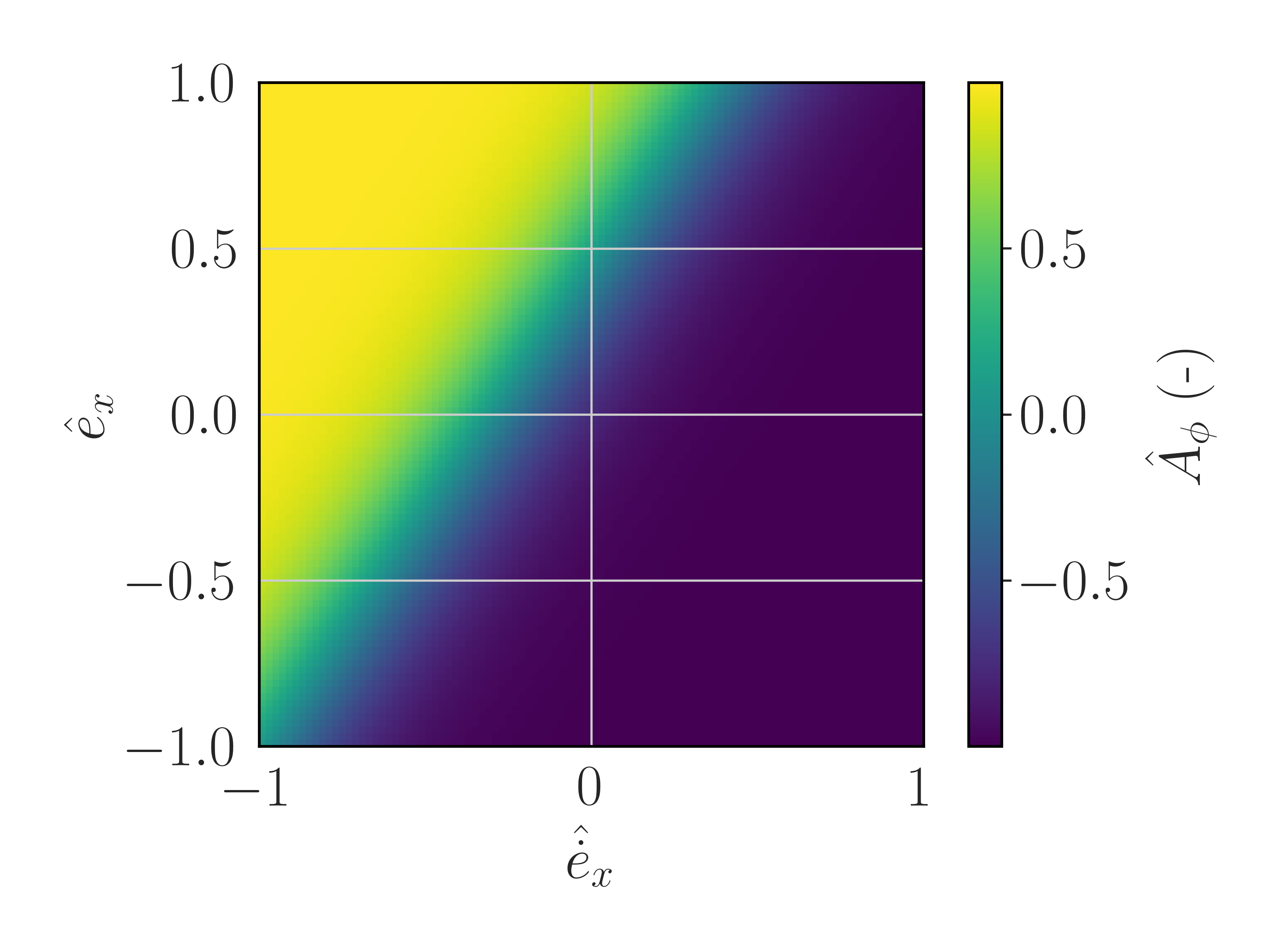
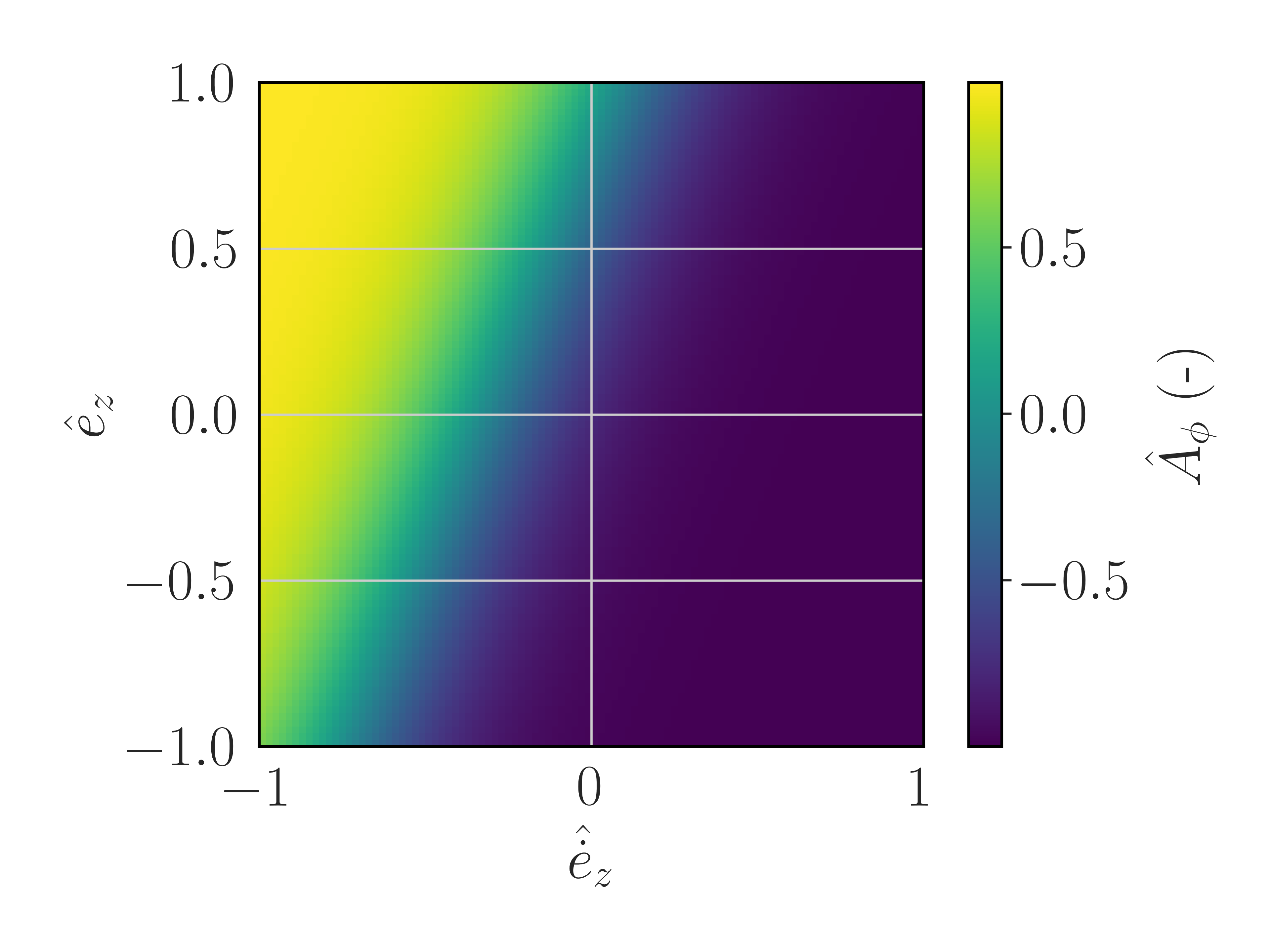

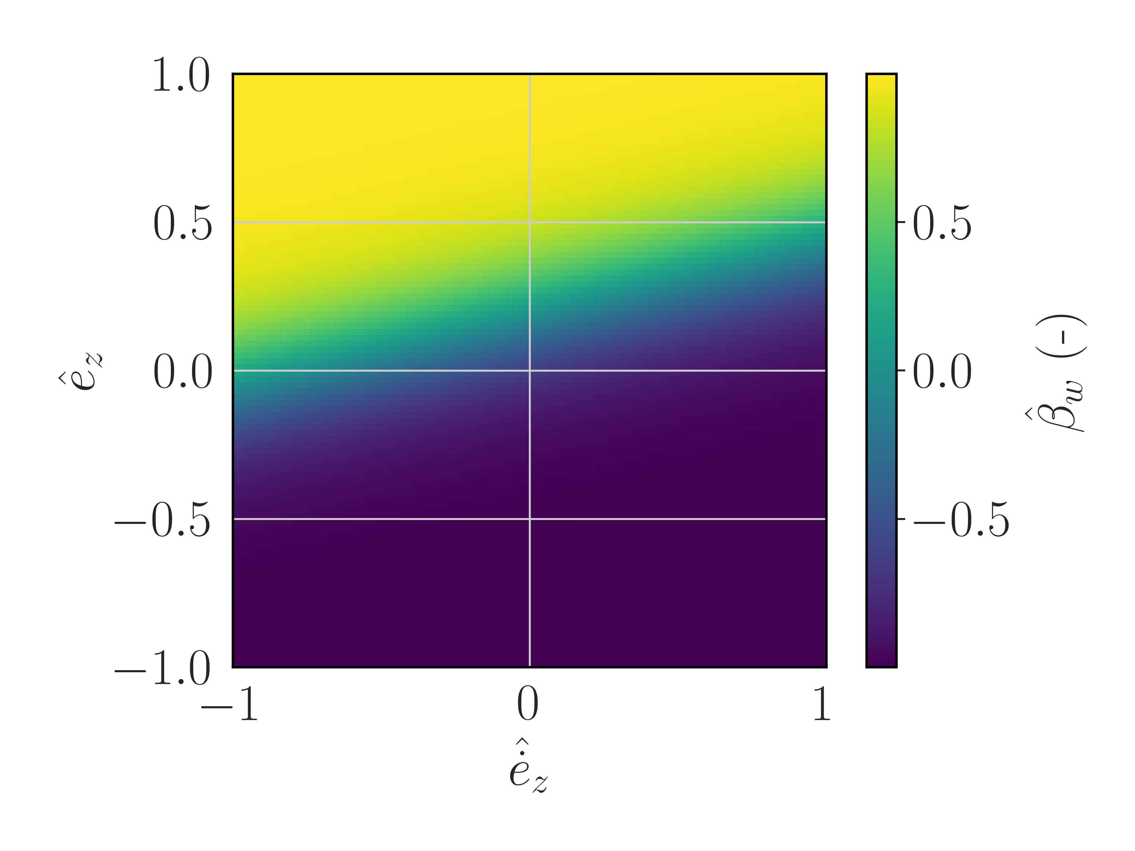

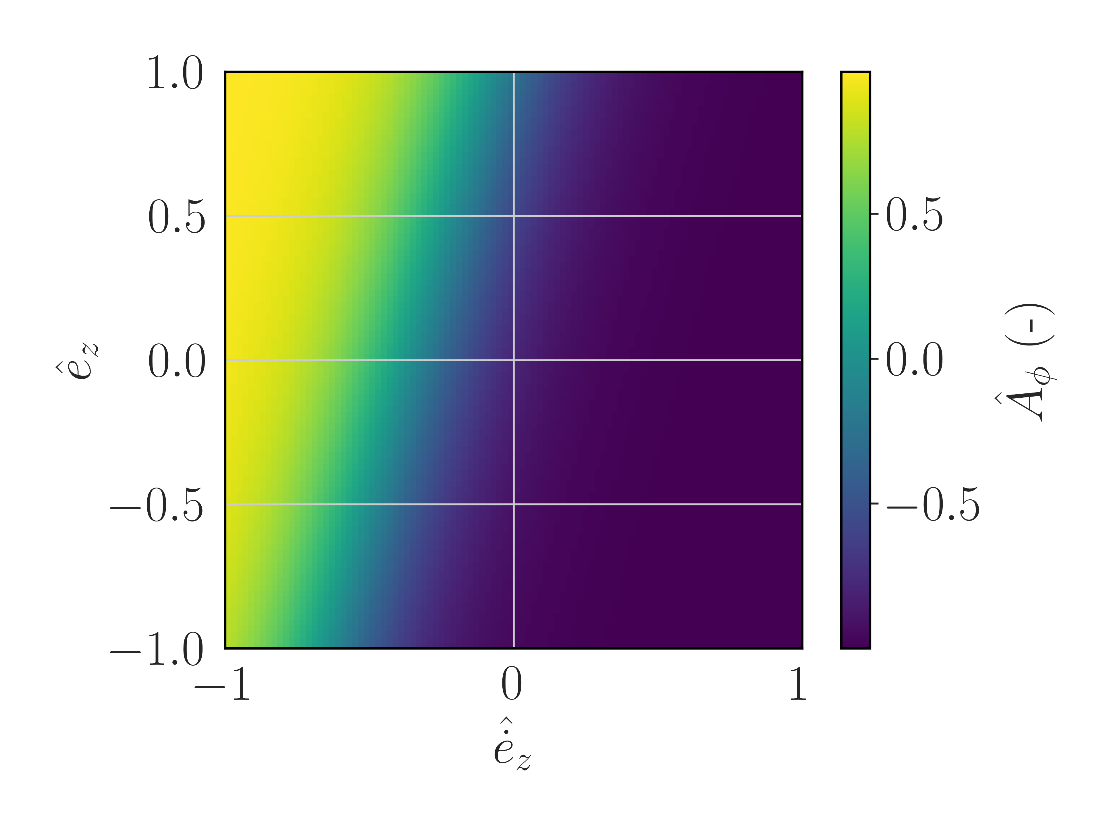
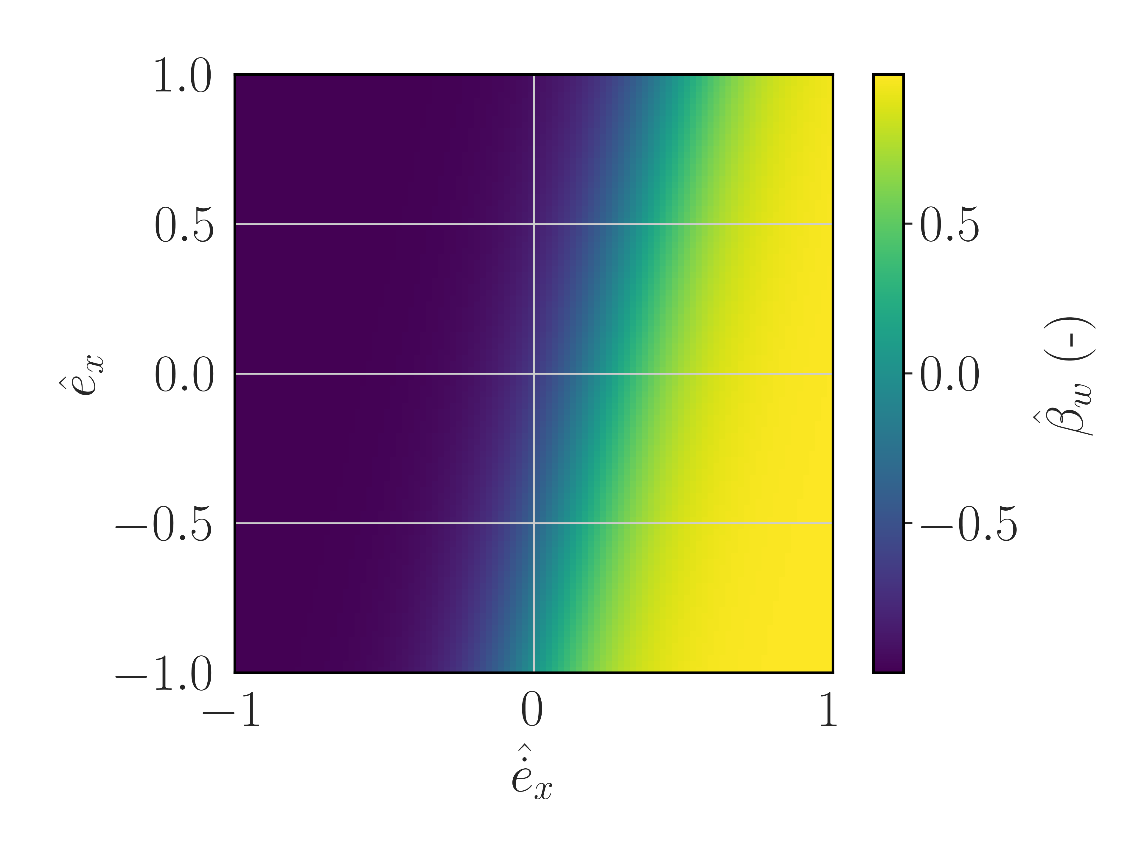
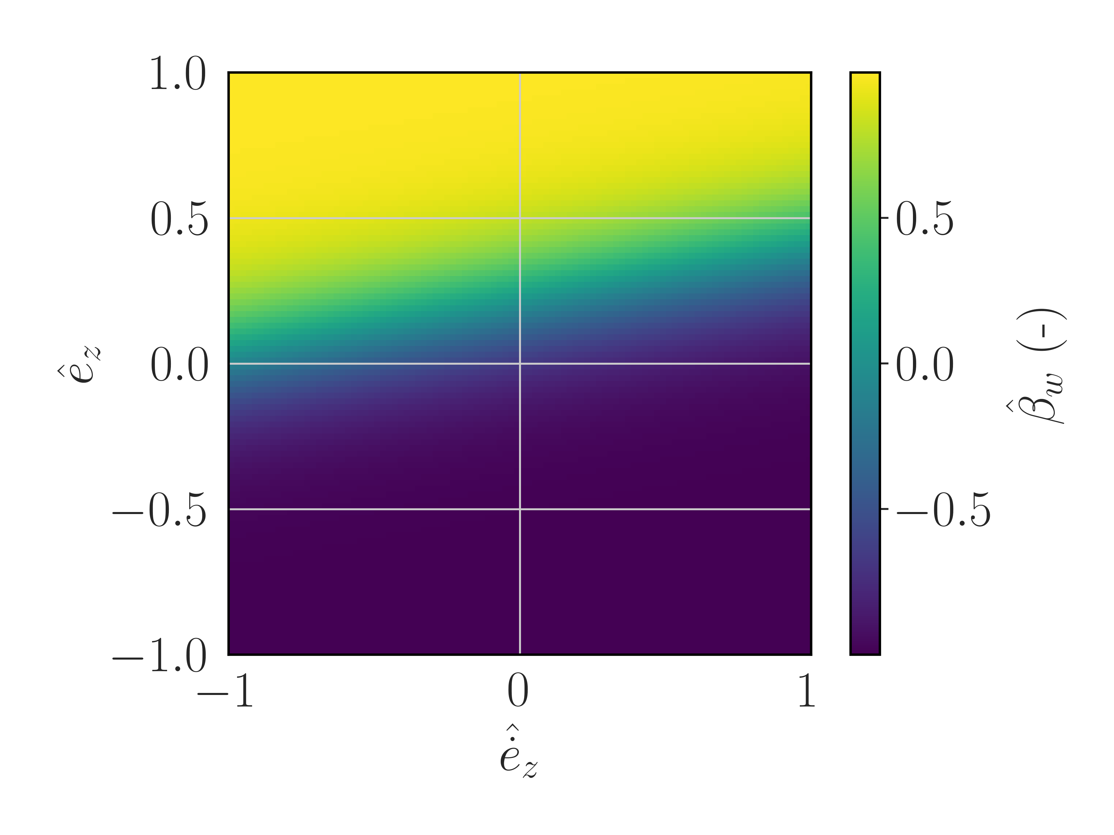
We conclude the FWMAV analysis presenting the robustness study of the model-free and model-based policies, shown in Figure 20. One-hundred episodes were run on the real environment for each policy and their costs are compared with violins plots (Figure 20(a)). Both sets of weights result in a small cost proving their capability to handle the random gust. The model-free policy manages to reach on average a lower cost and shows a slightly different distribution than the model-based policy, having two peaks at and , whereas the model-based shows a main peak in the middle, at . However, their differences are in the order , reinforcing the observation that the two have converged to a very similar policy. Lastly, The same procedure is then applied on the assimilation side, studying its robustness to varying operative conditions, as shown in Figure 20(b). It appears that the identified closure function is robust to different operative conditions, registering a mean cost of .
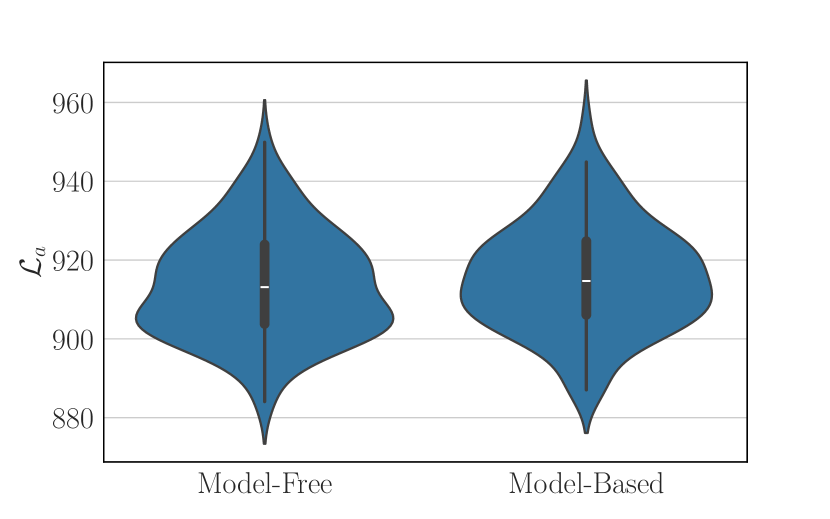
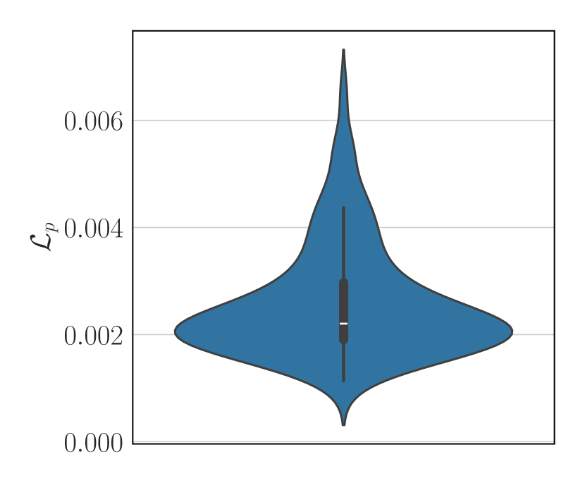
6.4 Thermal management of cryogenic storage
At last, we examine the RT results on the cryogenic thermal management test case.
The digital twin assimilation consists of identifying the weights which drive the heat transfer between the cryogenic tank and the environment, as well as the performance of the active TVS. For all simulations, this vector was initialized taking , with the units of the first two components being (W/m2K), and the last being (GPaskg2).
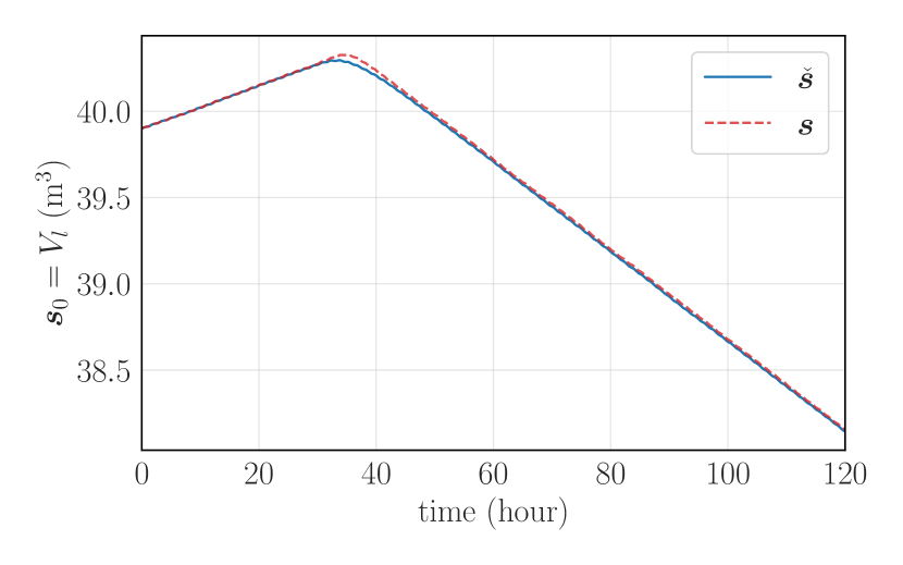
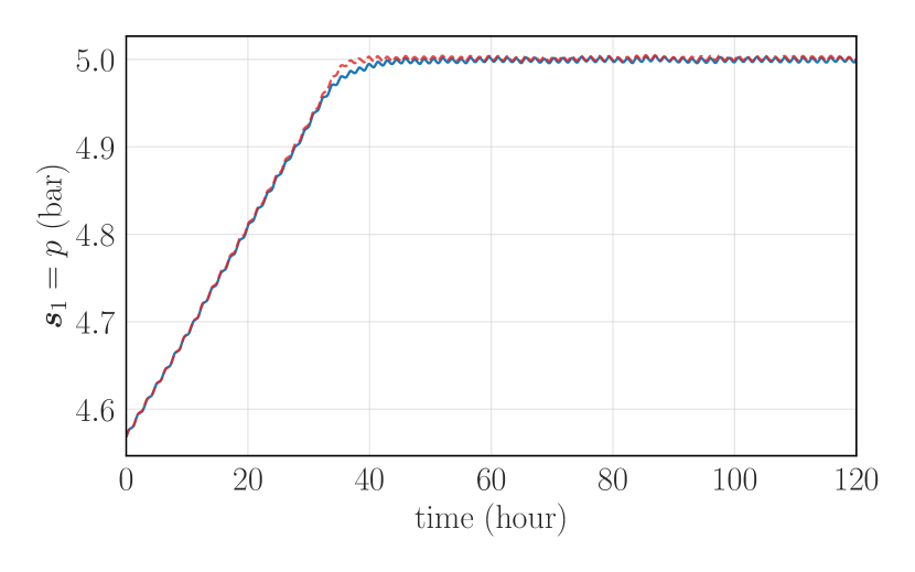
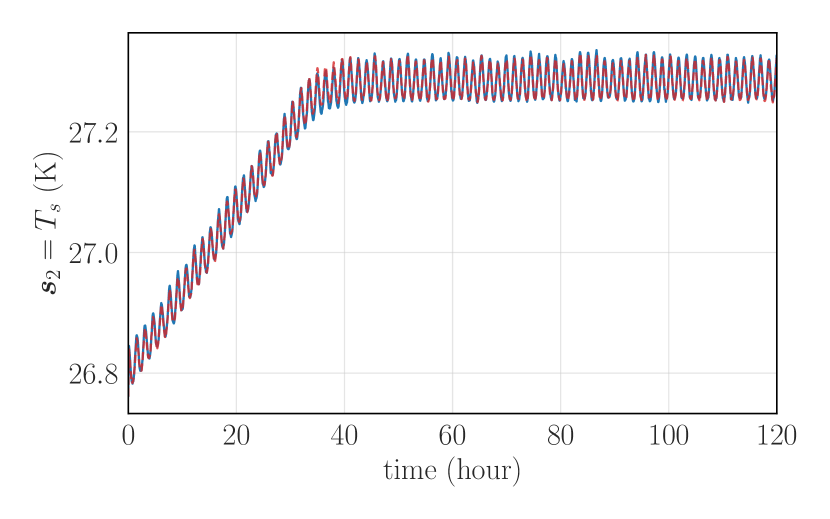
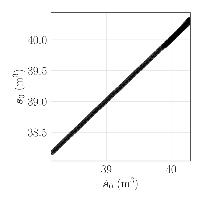
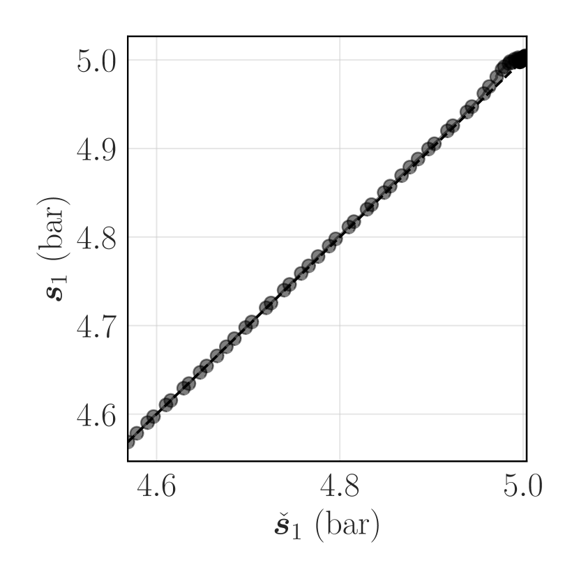
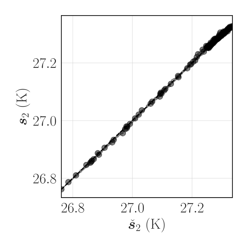
The agreement between the predicted state and the real one is presented in Figure 21, which shows both the time series of the real and predicted states (Figures 21(a) - 21(c)) and their direct comparison plotting one against the other (Figures 21(d) - 21(f)). All three components are successfully identified, even though slight deviations are found for and .
The control performances of the optimal parametrization, , extracted from the learning curve presented in Figure 10(d) are studied next. The current scenario involves an initial over-pressurized tank operating 0.4 bar above the reference . Figure 22 shows the time evolution of the real pressure and propellant mass over time, while the vented mass flow rate . Figures 22(b) and 22(c) show the control action over time and the corresponding pressure, respectively. Since the tank is initially in an over-pressurized state sufficiently far from , the valve was regulated to open to at its widest ( g/s) allowing the pressure to rapidly reduce until the target 5 bar are reached. This pressure drop is accompanied by a consumption of 87 kg over two roughly 45 hours. Once the target is reached, the active TVS regulates the pressure around this value. To do so, fluctuates between -50% and 25% around its midpoint due to changes in the heat due to the disturbance, although such variations are not seen in the pressure signal.
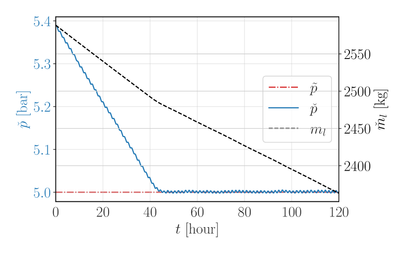
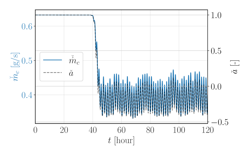
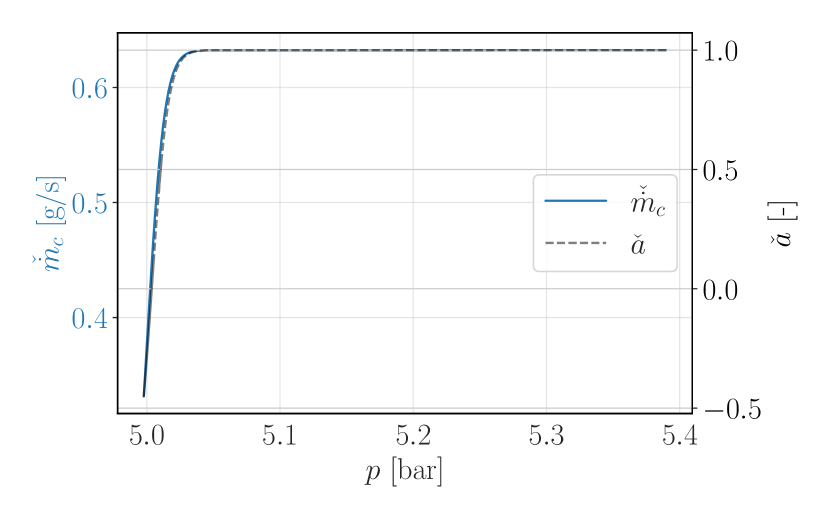
From these findings, we conclude that the control policy is able to completely control the tank pressure around its desired target value. However, the response time of the TVS is limited by the technical constraints assigned to the circulating pump, and Joule-Thomson valve. In addition, depending on the value assigned to the constant in 47, one could retrieve either faster or more fuel-efficient policies.
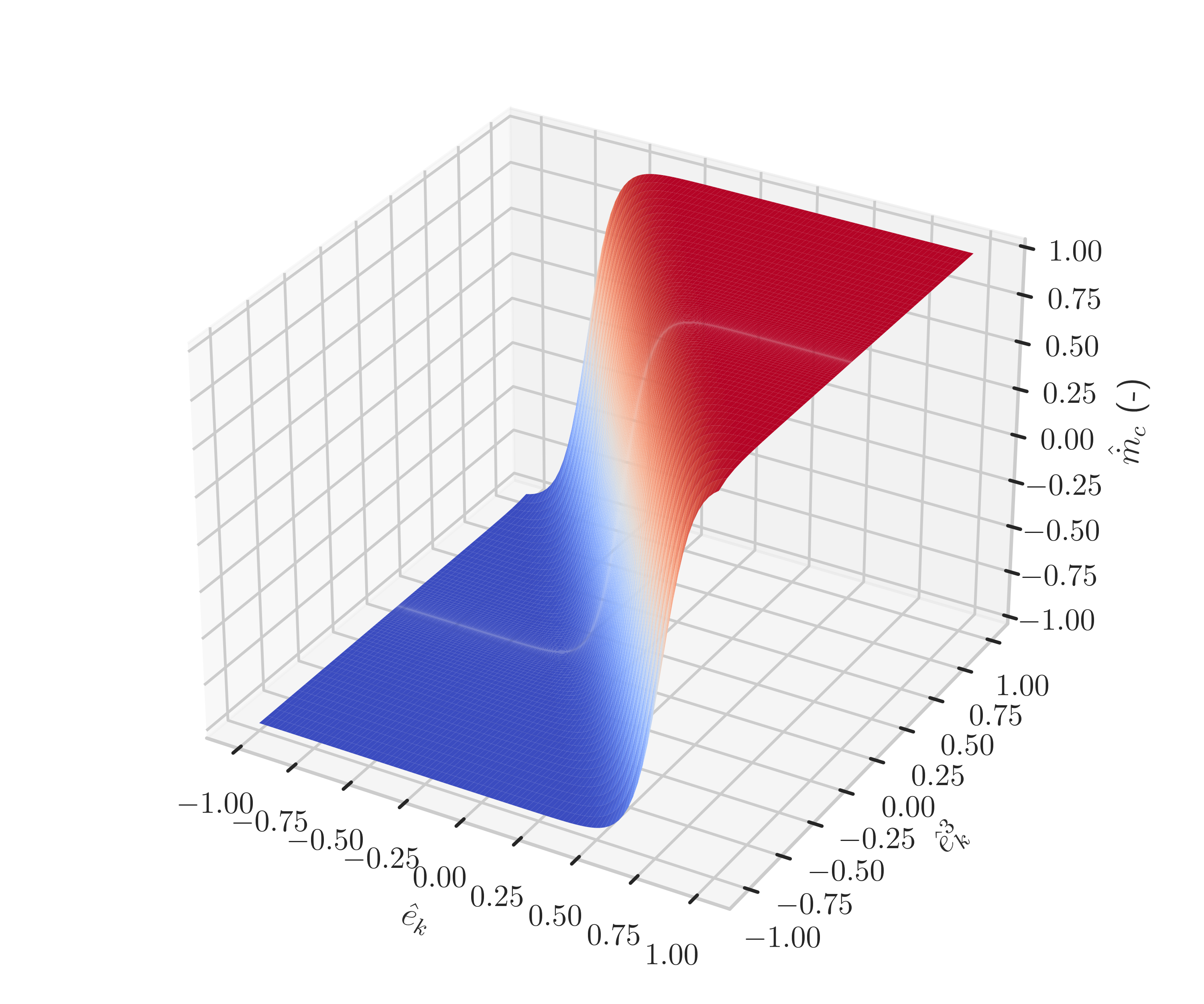
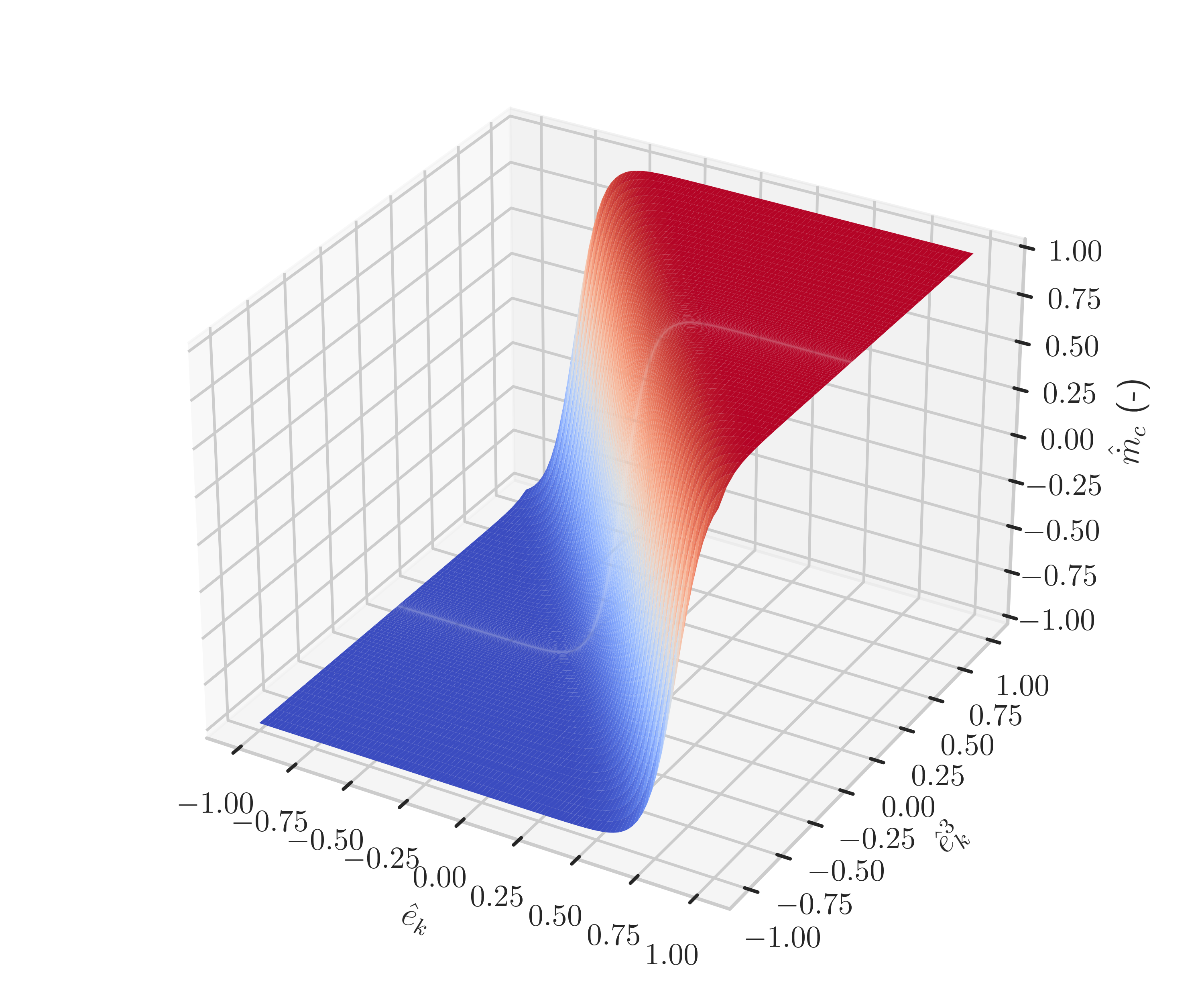
We inspect the two found policies in Figure 23. The two loops, model-based and model-free, converge to essentially the same parametrization. They show almost identical response to the possible input space, with very minor discrepancies in the inclination of the hyperbolic tangent. Lastly, the robustness of the assimilation and control loops concludes this overview. The procedure consists in evaluating the cost of the optimal weights and over observations unseen during the training phase. To this end, we carried out one-hundred simulations on random initial conditions and disturbances. For each of them, we computed the assimilation cost , as well as the control cost using the model-based and model-free policies. This investigation, summarized in the violin plots presented in Figures 24(a) and 24(b), proves that the weights obtained at the end of the learning phase are valid and robust even in unseen scenarios. Moreover, in contrast to what was observed in the wind turbine test case, the model-based and model-free weights are nearly identical, thus their performances are also identical as supported by Table 2 which shows a difference between the two control performances in the order of . This is likely a consequence of both approaches converging in the same region of the search space.
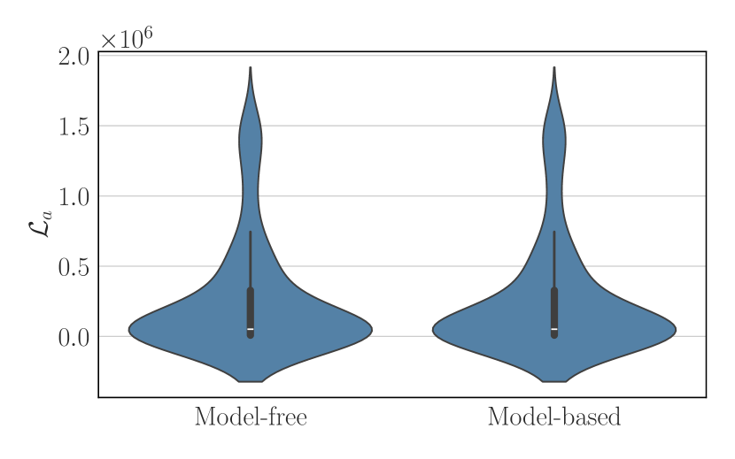
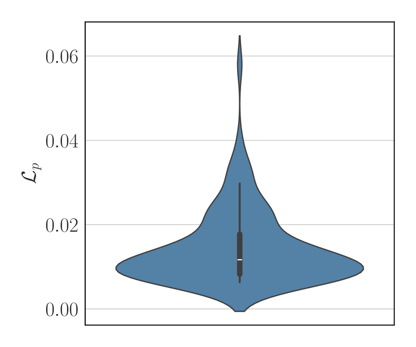
7 Conclusions and outlooks
We presented a novel framework to train physics-based digital twins from real-time data while at the same time training a control agent through a combination of model-free and model-based methods. We called this framework Reinforcement Twinning (RT), and we positioned it at the intersection between data assimilation, system identification and reinforcement learning. The digital twins are formulated as physics-based models relying on closure laws expressed as parametric functions. The parameters defining these closures are identified from real-time data using and adjoint-based data assimilation strategy.
We presented a novel framework to train physics-based digital twins from real-time data while at the same time training a control agent through a combination of model-free and model-based methods. We called this framework Reinforcement Twinning (RT) and positioned it at the intersection between data assimilation, system identification and reinforcement learning. The digital twins are formulated as physics-based models relying on closure laws expressed as parametric functions. The parameters defining these closures are identified from real-time data using an adjoint-based data assimilation strategy.
Similarly, the control agent acts on the system via a policy, also defined via parametric functions. The same adjoint-based framework is then used on the digital twin to identify the control policy and thus train the agent in the so-called “model-based” training. At the same time, a reinforcement learning approach using the Deep Deterministic Policy Gradient (DDPG) pursues the same task of training the control agent without using explicit knowledge of the system in the so-called “model-free” training. The “model-based” and the “model-free”” policies are then tested on the digital twin once this has reached satisfying predictive performances and the best-performing policy becomes the ”live policy” taken on the real system. We explored a first mechanism to let both the “model-based” and the “model-free” learn from the live policy and showed that this can create a virtuous loop in which both approaches lead to a sequence of improvements over the other.
We tested this novel framework on three widely different engineering systems: a wind turbine in a time-varying wind speed, a flapping-wing micro air vehicle travelling against gusts, and the thermal management of a cryogenic tank subject to time-varying heat loads. In these problems, the physics-based model of the digital twin is formulated as ODEs ensuring the compliance of predictions with fundamental principles (conservation of angular momentum in a wind turbine, Newton’s law in the drone’s trajectory and conservation of mass/energy within the cryogenic tank) and the closure law describe unmodelled physics (aerodynamic coefficients and heat transfer correlations).
The performance of the Reinforcement Twinning framework, both in training the digital twin and the controlling agent, proves the framework’s potential beyond any specific application. The merit stems from the complementary characteristics of the two approaches, the model-based being extremely sample-efficient but prone to fall stuck into local minima and the model-free being sample-inefficient but able to explore the parameter space better.
The paths towards future extensions are many. On the one hand, we could introduce a more advanced learning feedback mechanism between the model-free and the model-based methods, which is currently limited to a “cloning” procedure. This could allow, for example, different policy architecture between the two, unleashing the potential of reinforcement learning to handle arbitrarily complex policies in the form of an artificial neural network. On the other hand, we could introduce more sophisticated methods of integrating the digital twin in the training of the model-free loop, for instance, by using the virtual environment to boost the training of the critic network with strategies akin to traditional model-based reinforcement learning.
Nevertheless, these preliminary results open the path towards further hybridization of model-based and model-free methods and, more broadly, between traditional engineering and machine learning. Such a combination is essential to profit from the ever-growing availability of real-time data to achieve excellent predictive and control capabilities without sacrificing interpretability.
References
- Raw [2000] Tutorial overview of model predictive control. IEEE Control Syst 2000;20(3):38–52. URL: https://ieeexplore.ieee.org/document/845037/. doi:10.1109/37.845037.
- Abarbanel et al. [2017] Abarbanel H, Rozdeba P, Shirman S. Machine learning, deepest learning: Statistical data assimilation problems. 2017. arXiv:1707.01415.
- Abbas et al. [2020] Abbas NJ, Wright A, Pao L. An update to the national renewable energy laboratory baseline wind turbine controller. In: Journal of Physics: Conference Series. IOP Publishing; volume 1452; 2020. p. 012002.
- Ahmed et al. [2020] Ahmed SE, Pawar S, San O. PyDA: A hands-on introduction to dynamical data assimilation with python. Fluids 2020;5(4):225. doi:10.3390/fluids5040225.
- Ammar et al. [2022] Ammar A, Nassereddine H, AbdulBaky N, AbouKansour A, Tannoury J, Urban H, Schranz C. Digital Twins in the Construction Industry: A Perspective of Practitioners and Building Authority. Front Built Environ 2022;8:834671. URL: https://www.frontiersin.org/articles/10.3389/fbuil.2022.834671/full. doi:10.3389/fbuil.2022.834671.
- Andersson et al. [2019] Andersson C, Ribeiro AH, Tiels K, Wahlstrom N, Schon TB. Deep convolutional networks in system identification. In: 2019 IEEE 58th Conference on Decision and Control (CDC). IEEE; 2019. doi:10.1109/cdc40024.2019.9030219.
- Arcucci et al. [2021] Arcucci R, Zhu J, Hu S, Guo YK. Deep data assimilation: Integrating deep learning with data assimilation. Applied Sciences 2021;11(3):1114. doi:10.3390/app11031114.
- Asch et al. [2016] Asch M, Bocquet M, Nodet M. Data Assimilation. Society for Industrial and Applied Mathematics, 2016. doi:10.1137/1.9781611974546.
- Astrom and Wittenmark [1994] Astrom KJ, Wittenmark B. Adaptive Control. 2nd ed. Prentice Hall, 1994.
- Ayed et al. [2019] Ayed I, de Bézenac E, Pajot A, Brajard J, Gallinari P. Learning Dynamical Systems from Partial Observations. 2019. URL: http://arxiv.org/abs/1902.11136; arXiv:1902.11136 [physics].
- Baker et al. [2019] Baker N, Alexander F, Bremer T, Hagberg A, Kevrekidis Y, Najm H, Parashar M, Patra A, Sethian J, Wild S, Willcox K, Lee S. Workshop report on basic research needs for scientific machine learning: Core technologies for artificial intelligence 2019;URL: https://www.osti.gov/biblio/1478744. doi:10.2172/1478744.
- Barricelli et al. [2019] Barricelli BR, Casiraghi E, Fogli D. A survey on digital twin: Definitions, characteristics, applications, and design implications. IEEE Access 2019;7:167653--7. doi:10.1109/access.2019.2953499.
- Barsi [2011] Barsi S. Ventless Pressure Control of Cryogenic Storage Tanks. Ph.D. thesis; CASE Western Reserve University; 2011.
- Barsi and Kassemi [2013a] Barsi S, Kassemi M. Investigation of tank pressurization and pressure control—part i: Experimental study. Journal of Thermal Science and Engineering Applications 2013a;5(4). doi:10.1115/1.4023891.
- Barsi and Kassemi [2013b] Barsi S, Kassemi M. Investigation of tank pressurization and pressure control—part II: Numerical modeling. Journal of Thermal Science and Engineering Applications 2013b;5(4). doi:10.1115/1.4023892.
- van Beek et al. [2023] van Beek A, Karkaria VN, Chen W. Digital twins for the designs of systems: a perspective. Structural and Multidisciplinary Optimization 2023;66(3). doi:10.1007/s00158-023-03488-x.
- Bertsekas [2019] Bertsekas D. Reinforcement Learning and Optimal Control. Athena Scientific, 2019.
- Bhatnagar et al. [2009] Bhatnagar S, Sutton RS, Ghavamzadeh M, Lee M. Natural actor–critic algorithms. Automatica 2009;45(11):2471--82. URL: https://linkinghub.elsevier.com/retrieve/pii/S0005109809003549. doi:10.1016/j.automatica.2009.07.008.
- Bhowmik and Spee [1999] Bhowmik S, Spee R. Performance Optimization for Doubly Fed Wind Power Generation Systems. IEEE TRANSACTIONS ON INDUSTRY APPLICATIONS 1999;35(4).
- Bianchi et al. [2007] Bianchi FD, De Battista H, Mantz RJ. Wind turbine control systems: principles, modelling and gain scheduling design. volume 19. Springer, 2007.
- Bocquet [2011] Bocquet M. Ensemble kalman filtering without the intrinsic need for inflation. Nonlinear Processes in Geophysics 2011;18(5):735--50. doi:10.5194/npg-18-735-2011.
- Bocquet et al. [2019] Bocquet M, Brajard J, Carrassi A, Bertino L. Data assimilation as a deep learning tool to infer ode representations of dynamical models. 2019. .
- Bocquet and Farchi [2023] Bocquet M, Farchi A. Introduction to the principles and methods of data assimilation in the geosciences. Technical Report; École des Ponts ParisTech; 2023.
- Boedecker et al. [2014a] Boedecker J, Springenberg JT, Wülfing J, Riedmiller M. Approximate real-time optimal control based on sparse gaussian process models. In: 2014 IEEE Symposium on Adaptive Dynamic Programming and Reinforcement Learning (ADPRL). 2014a. p. 1--8. doi:10.1109/ADPRL.2014.7010608.
- Boedecker et al. [2014b] Boedecker J, Springenberg JT, Wülfing J, Riedmiller M. Approximate real-time optimal control based on sparse gaussian process models. In: 2014 IEEE Symposium on Adaptive Dynamic Programming and Reinforcement Learning (ADPRL). 2014b. p. 1--8. doi:10.1109/ADPRL.2014.7010608.
- Bossanyi [2000] Bossanyi EA. The Design of closed loop controllers for wind turbines. Wind Energ 2000;3(3):149--63. URL: https://onlinelibrary.wiley.com/doi/10.1002/we.34. doi:10.1002/we.34.
- Bradley [2019] Bradley AM. Pde-constrained optimization and the adjoint method 2019;.
- Brajard et al. [2020] Brajard J, Carassi A, Bocquet M, Bertino L. Combining data assimilation and machine learning to emulate a dynamical model from sparse and noisy observations: a case study with the Lorenz 96 model. Journal of Computational Science 2020;44:101171. URL: http://arxiv.org/abs/2001.01520. doi:10.1016/j.jocs.2020.101171; arXiv:2001.01520 [physics, stat].
- Branlard et al. [2023] Branlard E, Jonkman J, Brown C, Zang J. A digital-twin solution for floating offshore wind turbines validated using a full-scale prototype. Wind Energy Science Discussions 2023;2023:1--34. URL: https://wes.copernicus.org/preprints/wes-2023-50/. doi:10.5194/wes-2023-50.
- Buizza et al. [2022] Buizza C, Casas CQ, Nadler P, Mack J, Marrone S, Titus Z, Cornec CL, Heylen E, Dur T, Ruiz LB, Heaney C, Lopez JAD, Kumar KS, Arcucci R. Data learning: Integrating data assimilation and machine learning. Journal of Computational Science 2022;58:101525. doi:10.1016/j.jocs.2021.101525.
- Cai et al. [2021] Cai X, Kolomenskiy D, Nakata T, Liu H. A cfd data-driven aerodynamic model for fast and precise prediction of flapping aerodynamics in various flight velocities. Journal of Fluid Mechanics 2021;915:A114.
- Canaday et al. [2020] Canaday D, Pomerance A, Gauthier DJ. Model-free control of dynamical systems with deep reservoir computing. 2020. arXiv:2010.02285.
- Cao et al. [2003] Cao Y, Li S, Petzold L, Serban R. Adjoint sensitivity analysis for differential-algebraic equations: The adjoint DAE system and its numerical solution. SIAM Journal on Scientific Computing 2003;24(3):1076--89. doi:10.1137/s1064827501380630.
- Carrassi et al. [2017] Carrassi A, Bocquet M, Bertino L, Evensen G. Data assimilation in the geosciences - an overview on methods, issues and perspectives. 2017. arXiv:1709.02798.
- Cengel and Ghajar [2019] Cengel Y, Ghajar A. Heat and Mass Transfer: Fundamentals and Applications. 6th ed. McGraw Hill, 2019.
- Chai and Wilhite [2014] Chai PR, Wilhite AW. Cryogenic thermal system analysis for orbital propellant depot. 2014. URL: https://linkinghub.elsevier.com/retrieve/pii/S0094576514001738. doi:10.1016/j.actaastro.2014.05.013.
- Chang and Lin [2011] Chang CC, Lin CJ. LIBSVM. ACM Transactions on Intelligent Systems and Technology 2011;2(3):1--27. doi:10.1145/1961189.1961199.
- Chatzilygeroudis et al. [2019] Chatzilygeroudis K, Vassiliades V, Stulp F, Calinon S, Mouret JB. A survey on policy search algorithms for learning robot controllers in a handful of trials. 2019. arXiv:1807.02303.
- Chen et al. [2018] Chen RTQ, Rubanova Y, Bettencourt J, Duvenaud D. Neural ordinary differential equations. In: Proceedings of the 32nd International Conference on Neural Information Processing Systems. Red Hook, NY, USA: Curran Associates Inc.; NIPS’18; 2018. p. 6572–6583.
- Chen et al. [1990] Chen S, Billings S, Grant P. Non-linear system identification using neural networks. International Journal of Control 1990;51(6):1191--214. doi:10.1080/00207179008934126.
- Cheng et al. [2016] Cheng B, Tobalske BW, Powers DR, Hedrick TL, Wethington SM, Chiu GT, Deng X. Flight mechanics and control of escape manoeuvres in hummingbirds. i. flight kinematics. Journal of Experimental Biology 2016;219(22):3518--31.
- Cheng et al. [2023] Cheng S, Quilodran-Casas C, Ouala S, Farchi A, Liu C, Tandeo P, Fablet R, Lucor D, Iooss B, Brajard J, Xiao D, Janjic T, Ding W, Guo Y, Carrassi A, Bocquet M, Arcucci R. Machine learning with data assimilation and uncertainty quantification for dynamical systems: a review. 2023. URL: http://arxiv.org/abs/2303.10462; arXiv:2303.10462 [cs].
- Chinesta et al. [2020] Chinesta F, Cueto E, Abisset-Chavanne E, Duval JL, Khaldi FE. Virtual, Digital and Hybrid Twins: A New Paradigm in Data-Based Engineering and Engineered Data. Arch Computat Methods Eng 2020;27(1):105--34. URL: http://link.springer.com/10.1007/s11831-018-9301-4. doi:10.1007/s11831-018-9301-4.
- Deisenroth and Rasmussen [2011] Deisenroth M, Rasmussen C. Pilco: A model-based and data-efficient approach to policy search. 2011. p. 465--72.
- Dickinson et al. [1999] Dickinson MH, Lehmann FO, Sane SP. Wing rotation and the aerodynamic basis of insect flight. Science 1999;284(5422):1954--60.
- Dimet et al. [2016] Dimet FXL, Navon IM, Ştefănescu R. Variational data assimilation: Optimization and optimal control. In: Data Assimilation for Atmospheric, Oceanic and Hydrologic Applications (Vol. III). Springer International Publishing; 2016. p. 1--53. doi:10.1007/978-3-319-43415-5_1.
- Errico [1997] Errico RM. What is an adjoint model? Bulletin of the American Meteorological Society 1997;78(11).
- Evensen [2009] Evensen G. Data Assimilation: The Ensemble Kalman Filter. 2nd ed. Spinger, 2009.
- Fahim et al. [2022] Fahim M, Sharma V, Cao TV, Canberk B, Duong TQ. Machine learning-based digital twin for predictive modeling in wind turbines. IEEE Access 2022;10:14184--94. URL: https://api.semanticscholar.org/CorpusID:246420062.
- Fei et al. [2019] Fei F, Tu Z, Yang Y, Zhang J, Deng X. Flappy hummingbird: An open source dynamic simulation of flapping wing robots and animals. In: 2019 International Conference on Robotics and Automation (ICRA). IEEE; 2019. p. 9223--9.
- Geer [2021] Geer AJ. Learning earth system models from observations: machine learning or data assimilation? Philosophical Transactions of the Royal Society A: Mathematical, Physical and Engineering Sciences 2021;379(2194). doi:10.1098/rsta.2020.0089.
- Gonzalez and Yu [2018] Gonzalez J, Yu W. Non-linear system modeling using LSTM neural networks. IFAC-PapersOnLine 2018;51(13):485--9. doi:10.1016/j.ifacol.2018.07.326.
- Goodfellow et al. [2016] Goodfellow I, Bengio Y, Courville A, Bengio Y. Deep learning. volume 1. MIT press Cambridge, 2016.
- Haarnoja et al. [2018] Haarnoja T, Zhou A, Abbeel P, Levine S. Soft actor-critic: Off-policy maximum entropy deep reinforcement learning with a stochastic actor. 2018. arXiv:1801.01290.
- Haghshenas et al. [2023] Haghshenas A, Hasan A, Osen O, Mikalsen ET. Predictive digital twin for offshore wind farms. Energy Informatics 2023;6(1):1--26.
- Haider et al. [2020] Haider N, Shahzad A, Qadri MNM, Shah SIA. Recent progress in flapping wings for micro aerial vehicle applications. Proceedings of the Institution of Mechanical Engineers, Part C: Journal of Mechanical Engineering Science 2020;235(2):245--64. doi:10.1177/0954406220917426.
- Hastings et al. [2005] Hastings L, Tucker S, Flachbart R, Hedayat A, Nelson S. Marshall space flight center in-space cryogenic fluid management program overview. In: 41st AIAA/ASME/SAE/ASEE Joint Propulsion Conference and Exhibit. American Institute of Aeronautics and Astronautics; 2005. doi:10.2514/6.2005-3561.
- Hastings et al. [2003] Hastings LJ, Flachbart R, Martin J, Hedayat A, Fazah M, Lak T, Nguyen H, Bailey J. Spray Bar Zero-Gravity Vent System for On-Orbit Liquid Hydrogen Storage. Technical Memorandum (TM) NASA/TM-2003-212926; National Aeronautics and Space Administration, Marshall Space Flight Center; Alabama 35812; 2003. URL: https://ntrs.nasa.gov/api/citations/20040000092/downloads/20040000092.pdf.
- Hedengren et al. [2014] Hedengren JD, Shishavan RA, Powell KM, Edgar TF. Nonlinear modeling, estimation and predictive control in APMonitor. Computers & Chemical Engineering 2014;70:133--48. URL: https://linkinghub.elsevier.com/retrieve/pii/S0098135414001306. doi:10.1016/j.compchemeng.2014.04.013.
- Hochreiter and Schmidhuber [1997] Hochreiter S, Schmidhuber J. Long short-term memory. Neural Computation 1997;9(8):1735--80. doi:10.1162/neco.1997.9.8.1735.
- Howlader et al. [2010] Howlader AM, Urasaki N, Uchida K, Yona A, Senjyu T, Kim CH, Saber AY. Parameter Identification of Wind Turbine for Maximum Power-point Tracking Control. Electric Power Components and Systems 2010;38(5):603--14. URL: http://www.tandfonline.com/doi/abs/10.1080/15325000903376974. doi:10.1080/15325000903376974.
- Hunt et al. [1992] Hunt K, Sbarbaro D, Żbikowski R, Gawthrop P. Neural networks for control systems—a survey. Automatica 1992;28(6):1083--112. URL: https://www.sciencedirect.com/science/article/pii/000510989290053I. doi:https://doi.org/10.1016/0005-1098(92)90053-I.
- Imai et al. [2020] Imai R, Nishida K, Kawanami O, Umemura Y, Himeno T. Ground based experiment and numerical calculation on thermodynamic vent system in propellant tank for future cryogenic propulsion system. Cryogenics 2020;109:103095. doi:10.1016/j.cryogenics.2020.103095.
- Jaeger and Haas [2004] Jaeger H, Haas H. Harnessing nonlinearity: Predicting chaotic systems and saving energy in wireless communication. Science 2004;304(5667):78--80. doi:10.1126/science.1091277.
- Jiang et al. [2021] Jiang W, Sun P, Li P, Zuo Z, Huang Y. Transient thermal behavior of multi-layer insulation coupled with vapor cooled shield used for liquid hydrogen storage tank. Energy 2021;231:120859. doi:10.1016/j.energy.2021.120859.
- Johnson [2004] Johnson KE. Adaptive torque control of variable speed wind turbines. University of Colorado at Boulder, 2004.
- Johnson [2006] Johnson KE. Control of variable-speed wind turbines: standard and adaptive techniques for maximizing energy capture. IEEE Control Systems Magazine 2006;26(3):70--81.
- Jonkman [2006] Jonkman BJ. TurbSim user’s guide. Technical Report; National Renewable Energy Lab.(NREL), Golden, CO (United States); 2006.
- Jonkman et al. [2009] Jonkman J, Butterfield S, Musial W, Scott G. Definition of a 5-MW reference wind turbine for offshore system development. Technical Report; National Renewable Energy Lab.(NREL), Golden, CO (United States); 2009.
- Kalnay et al. [2007] Kalnay E, Li H, Miyoshi T, Yang SC, Ballabrera-Poy J. 4-d-var or ensemble kalman filter? Tellus A: Dynamic Meteorology and Oceanography 2007;59(5):758. doi:10.1111/j.1600-0870.2007.00261.x.
- Khandelwal et al. [2021] Khandelwal P, Nadler P, Arcucci R, Knottenbelt W, Guo YK. A scalable inference method for large dynamic economic systems. 2021. arXiv:2110.14346.
- Kruyt et al. [2014] Kruyt JW, Quicazán-Rubio EM, Van Heijst GF, Altshuler DL, Lentink D. Hummingbird wing efficacy depends on aspect ratio and compares with helicopter rotors. Journal of the royal society interface 2014;11(99):20140585.
- Kurutach et al. [2018] Kurutach T, Clavera I, Duan Y, Tamar A, Abbeel P. Model-ensemble trust-region policy optimization. arXiv preprint arXiv:180210592 2018;.
- Lahoz et al. [2010] Lahoz W, Khattatov B, Menard R, editors. Data Assimilation. Springer Berlin Heidelberg, 2010. doi:10.1007/978-3-540-74703-1.
- Laks et al. [2009] Laks JH, Pao LY, Wright AD. Control of wind turbines: Past, present, and future. In: 2009 American Control Conference. IEEE; 2009. doi:10.1109/acc.2009.5160590.
- LeCun et al. [1989] LeCun Y, Boser B, Denker JS, Henderson D, Howard RE, Hubbard W, Jackel LD. Backpropagation applied to handwritten zip code recognition. Neural Computation 1989;1(4):541--51. doi:10.1162/neco.1989.1.4.541.
- Lee et al. [2016] Lee Y, Lua KB, Lim T, Yeo K. A quasi-steady aerodynamic model for flapping flight with improved adaptability. Bioinspiration & biomimetics 2016;11(3):036005.
- Leishman [2002] Leishman JG. Challenges in modelling the unsteady aerodynamics of wind turbines. Wind Energy: An International Journal for Progress and Applications in Wind Power Conversion Technology 2002;5(2-3):85--132.
- Lemmon et al. [2018] Lemmon EW, Bell IH, Huber ML, McLinden MO. NIST Standard Reference Database 23: Reference Fluid Thermodynamic and Transport Properties-REFPROP, Version 10.0, National Institute of Standards and Technology. 2018. URL: https://www.nist.gov/srd/refprop. doi:https://doi.org/10.18434/T4/1502528.
- Lillicrap et al. [2019] Lillicrap TP, Hunt JJ, Pritzel A, Heess N, Erez T, Tassa Y, Silver D, Wierstra D. Continuous control with deep reinforcement learning. 2019. arXiv:1509.02971.
- Lin et al. [1991] Lin C, Dresar N, Hasan M. Pressure control analysis of cryogenic storage systems. Journal of Propulsion and Power 1991;20. doi:10.2514/1.10387.
- Liu and MacArt [2023] Liu X, MacArt JF. Adjoint-based machine learning for active flow control. 2023. arXiv:2307.09980.
- Liu and Wang [2021] Liu XY, Wang JX. Physics-informed dyna-style model-based deep reinforcement learning for dynamic control. 2021. doi:10.1098/rspa.2021.0618. arXiv:2108.00128.
- Ljung [2008] Ljung L. Perspectives on system identification. IFAC Proceedings Volumes 2008;41(2):7172--84. doi:10.3182/20080706-5-kr-1001.01215.
- Ljung et al. [2020] Ljung L, Andersson CR, Tiels K, Schön TB. Deep learning and system identification. IFAC-PapersOnLine 2020;URL: https://api.semanticscholar.org/CorpusID:226118683.
- Lorenc [1986] Lorenc AC. Analysis methods for numerical weather prediction. Quarterly Journal of the Royal Meteorological Society 1986;112(474):1177--94. doi:10.1002/qj.49711247414.
- Lorenc et al. [2015] Lorenc AC, Bowler NE, Clayton AM, Pring SR, Fairbairn D. Comparison of hybrid-4denvar and hybrid-4dvar data assimilation methods for global NWP. Monthly Weather Review 2015;143(1):212--29. doi:10.1175/mwr-d-14-00195.1.
- Luo et al. [2022a] Luo FM, Xu T, Lai H, Chen XH, Zhang W, Yu Y. A survey on model-based reinforcement learning. 2022a. URL: http://arxiv.org/abs/2206.09328. doi:10.48550/arXiv.2206.09328. arXiv:2206.09328 [cs].
- Luo et al. [2022b] Luo FM, Xu T, Lai H, Chen XH, Zhang W, Yu Y. A survey on model-based reinforcement learning. 2022b. arXiv:2206.09328.
- Lutter et al. [2019] Lutter M, Ritter C, Peters J. Deep lagrangian networks: Using physics as model prior for deep learning. 2019. arXiv:1907.04490.
- Lutter et al. [2020] Lutter M, Silberbauer J, Watson J, Peters J. Differentiable physics models for real-world offline model-based reinforcement learning. 2020. arXiv:2011.01734.
- Madhavan [1993] Madhavan P. Recurrent neural network for time series prediction. In: Proceedings of the 15th Annual International Conference of the IEEE Engineering in Medicine and Biology Society. IEEE; 1993. doi:10.1109/iembs.1993.978527.
- Marques et al. [2023] Marques P, Ahizi S, Mendez MA. Real Time Data Assimilation for the Thermodynamic Modeling of a Cryogenic Fuel Tank. In: 36th International Conference on Efficiency, Cost, Optimization, Simulation and Environmental Impact of Energy Systems (ECOS 2023). Las Palmas De Gran Canaria, Spain: ECOS 2023; 2023. p. 1041--52. URL: http://www.proceedings.com/069564-0095.html. doi:10.52202/069564-0095.
- Mer et al. [2016a] Mer S, Fernandez D, Thibault JP, Corre C. Optimal design of a thermodynamic vent system for cryogenic propellant storage. Cryogenics 2016a;80:127--37. doi:10.1016/j.cryogenics.2016.09.012.
- Mer et al. [2016b] Mer S, Thibault JP, Corre C. Active insulation technique applied to the experimental analysis of a thermodynamic control system for cryogenic propellant storage. Journal of Thermal Science and Engineering Applications 2016b;8(2). doi:10.1115/1.4032761.
- Mnih et al. [2013a] Mnih V, Kavukcuoglu K, Silver D, Graves A, Antonoglou I, Wierstra D, Riedmiller M. Playing atari with deep reinforcement learning. 2013a. arXiv:1312.5602.
- Mnih et al. [2013b] Mnih V, Kavukcuoglu K, Silver D, Graves A, Antonoglou I, Wierstra D, Riedmiller M. Playing atari with deep reinforcement learning. 2013b. arXiv:http://arxiv.org/abs/1312.5602v1.
- Mnih et al. [2015] Mnih V, Kavukcuoglu K, Silver D, Rusu AA, Veness J, Bellemare MG, Graves A, Riedmiller M, Fidjeland AK, Ostrovski G, Petersen S, Beattie C, Sadik A, Antonoglou I, King H, Kumaran D, Wierstra D, Legg S, Hassabis D. Human-level control through deep reinforcement learning. Nature 2015;518(7540):529--33. doi:10.1038/nature14236.
- Moerland et al. [2022a] Moerland TM, Broekens J, Plaat A, Jonker CM. Model-based reinforcement learning: A survey. 2022a. URL: http://arxiv.org/abs/2006.16712. doi:10.48550/arXiv.2006.16712. arXiv:2006.16712 [cs, stat].
- Moerland et al. [2022b] Moerland TM, Broekens J, Plaat A, Jonker CM. Model-based reinforcement learning: A survey. 2022b. arXiv:2006.16712.
- Moriarty and Hansen [2005] Moriarty PJ, Hansen AC. AeroDyn theory manual. Technical Report; National Renewable Energy Lab., Golden, CO (US); 2005.
- Motil et al. [2007] Motil S, Meyer M, Tucker S. Cryogenic fluid management technologies for advanced green propulsion systems. In: 45th AIAA Aerospace Sciences Meeting and Exhibit. American Institute of Aeronautics and Astronautics; 2007. doi:10.2514/6.2007-343.
- Nadler et al. [2020] Nadler P, Arcucci R, Guo Y. A neural sir model for global forecasting. In: Alsentzer E, McDermott MBA, Falck F, Sarkar SK, Roy S, Hyland SL, editors. Proceedings of the Machine Learning for Health NeurIPS Workshop. PMLR; volume 136 of Proceedings of Machine Learning Research; 2020. p. 254--66. URL: https://proceedings.mlr.press/v136/nadler20a.html.
- Nagabandi et al. [2017] Nagabandi A, Kahn G, Fearing RS, Levine S. Neural network dynamics for model-based deep reinforcement learning with model-free fine-tuning. 2017. arXiv:1708.02596.
- Nelles [2001] Nelles O. Nonlinear System Identification. Springer Berlin Heidelberg, 2001. doi:10.1007/978-3-662-04323-3.
- Nicolao [2003] Nicolao GD. System identification : Problems and perspectives. In: 12th Workshop on Qualitative Reasoning. 2003. URL: https://api.semanticscholar.org/CorpusID:26963940.
- Norgaard et al. [2000] Norgaard M, Ravn O, Poulsen N, Hansen L. Neural Networks for Modelling and Control of Dynamic Systems. Advanced Textbooks in Control and Signal Processing. Springer London, 2000.
- Olatunji et al. [2021] Olatunji OO, Adedeji PA, Madushele N, Jen TC. Overview of digital twin technology in wind turbine fault diagnosis and condition monitoring. 2021 IEEE 12th International Conference on Mechanical and Intelligent Manufacturing Technologies (ICMIMT) 2021;:201--7URL: https://api.semanticscholar.org/CorpusID:236190314.
- Ortega-Jiménez and Dudley [2018] Ortega-Jiménez VM, Dudley R. Ascending flight and decelerating vertical glides in anna’s hummingbirds. Journal of Experimental Biology 2018;221(24):jeb191171.
- Panzarella et al. [2004] Panzarella C, Plachta D, Kassemi M. Pressure control of large cryogenic tanks in microgravity. 2004. URL: https://linkinghub.elsevier.com/retrieve/pii/S0011227504000633. doi:10.1016/j.cryogenics.2004.03.009.
- Panzarella and Kassemi [2003] Panzarella CH, Kassemi M. On the validity of purely thermodynamic descriptions of two-phase cryogenic fluid storage. 2003. URL: http://www.journals.cambridge.org/abstract_S0022112003004002. doi:10.1017/S0022112003004002.
- Pao and Johnson [2009] Pao LY, Johnson KE. A tutorial on the dynamics and control of wind turbines and wind farms. In: 2009 American Control Conference. IEEE; 2009. doi:10.1109/acc.2009.5160195.
- Pillonetto et al. [2023] Pillonetto G, Aravkin A, Gedon D, Ljung L, Ribeiro AH, Schön TB. Deep networks for system identification: a survey. 2023. arXiv:2301.12832.
- Pimenta et al. [2020] Pimenta F, Pacheco J, Branco CM, Teixeira CM, Magalhães F. Development of a digital twin of an onshore wind turbine using monitoring data. Journal of Physics: Conference Series 2020;1618(2):022065. URL: https://dx.doi.org/10.1088/1742-6596/1618/2/022065. doi:10.1088/1742-6596/1618/2/022065.
- Pino et al. [2023] Pino F, Schena L, Rabault J, Mendez MA. Comparative analysis of machine learning methods for active flow control. Journal of Fluid Mechanics 2023;958. doi:10.1017/jfm.2023.76.
- Pu and Kalnay [2018] Pu Z, Kalnay E. Numerical weather prediction basics: Models, numerical methods, and data assimilation. In: Handbook of Hydrometeorological Ensemble Forecasting. Springer Berlin Heidelberg; 2018. p. 1--31. doi:10.1007/978-3-642-40457-3_11-1.
- Puterman [1994] Puterman ML. Markov Decision Processes. Wiley, 1994. doi:10.1002/9780470316887.
- Qin et al. [2021] Qin X, Li P, Sun P, Huang Y. Testing and comparison of a thermodynamic vent system operating in different modes in a liquid nitrogen tank. Applied Thermal Engineering 2021;197:117393. doi:10.1016/j.applthermaleng.2021.117393.
- Rahman et al. [2022] Rahman A, Drgoňa J, Tuor A, Strube J. Neural ordinary differential equations for nonlinear system identification. 2022. arXiv:2203.00120.
- Raissi et al. [2019] Raissi M, Perdikaris P, Karniadakis GE. Physics-informed neural networks: A deep learning framework for solving forward and inverse problems involving nonlinear partial differential equations. Journal of Computational physics 2019;378:686--707.
- Ramesh and Ravindran [2023] Ramesh A, Ravindran B. Physics-informed model-based reinforcement learning. 2023. arXiv:2212.02179.
- Rasheed et al. [2019] Rasheed A, San O, Kvamsdal T. Digital Twin: Values, Challenges and Enablers. 2019. URL: http://arxiv.org/abs/1910.01719; arXiv:1910.01719 [eess].
- Rasmussen and Williams [2005] Rasmussen CE, Williams CKI. Gaussian Processes for Machine Learning. MIT Press Ltd, 2005.
- Routray et al. [2016] Routray A, Osuri KK, Pattanayak S, Mohanty UC. Introduction to data assimilation techniques and ensemble kalman filter. In: Advanced Numerical Modeling and Data Assimilation Techniques for Tropical Cyclone Prediction. Springer Netherlands; 2016. p. 307--30. doi:10.5822/978-94-024-0896-6_11.
- Saint-Drenan et al. [2020] Saint-Drenan YM, Besseau R, Jansen M, Staffell I, Troccoli A, Dubus L, Schmidt J, Gruber K, Simões SG, Heier S. A parametric model for wind turbine power curves incorporating environmental conditions. Renewable Energy 2020;157:754--68. URL: https://www.sciencedirect.com/science/article/pii/S0960148120306613. doi:https://doi.org/10.1016/j.renene.2020.04.123.
- Salzman [1996] Salzman JA. Fluid management in space-based systems. In: Engineering, Construction, and Operations in Space V. American Society of Civil Engineers; 1996. doi:10.1061/40177(207)71.
- Sane [2003] Sane SP. The aerodynamics of insect flight. Journal of experimental biology 2003;206(23):4191--208.
- Sane and Dickinson [2001] Sane SP, Dickinson MH. The control of flight force by a flapping wing: lift and drag production. Journal of experimental biology 2001;204(15):2607--26.
- Sastry and Isidori [1989] Sastry SS, Isidori A. Adaptive control of linearizable systems. IEEE Transactions on Automatic Control 1989;34(11):1123--31.
- Schaul et al. [2015] Schaul T, Quan J, Antonoglou I, Silver D. Prioritized experience replay. 2015. doi:10.48550/ARXIV.1511.05952.
- Schaul et al. [2016] Schaul T, Quan J, Antonoglou I, Silver D. Prioritized experience replay. 2016. arXiv:1511.05952.
- Schoukens and Ljung [2019] Schoukens J, Ljung L. Nonlinear system identification: A user-oriented road map. IEEE Control Systems 2019;39(6):28--99. doi:10.1109/mcs.2019.2938121.
- Schwenzer et al. [2021] Schwenzer M, Ay M, Bergs T, Abel D. Review on model predictive control: an engineering perspective. Int J Adv Manuf Technol 2021;117(5-6):1327--49. URL: https://link.springer.com/10.1007/s00170-021-07682-3. doi:10.1007/s00170-021-07682-3.
- Silver et al. [2016] Silver D, Huang A, Maddison CJ, Guez A, Sifre L, van den Driessche G, Schrittwieser J, Antonoglou I, Panneershelvam V, Lanctot M, Dieleman S, Grewe D, Nham J, Kalchbrenner N, Sutskever I, Lillicrap T, Leach M, Kavukcuoglu K, Graepel T, Hassabis D. Mastering the game of go with deep neural networks and tree search. Nature 2016;529(7587):484--9.
- Silver et al. [2018] Silver D, Hubert T, Schrittwieser J, Antonoglou I, Lai M, Guez A, Lanctot M, Sifre L, Kumaran D, Graepel T, Lillicrap T, Simonyan K, Hassabis D. A general reinforcement learning algorithm that masters chess, shogi, and go through self-play. Science 2018;362(6419):1140--4.
- Silver et al. [2014] Silver D, Lever G, Heess N, Degris T, Wierstra D, Riedmiller M. Deterministic Policy Gradient Algorithms 2014;.
- Sjöberg et al. [1994] Sjöberg J, Hjalmarsson H, Ljung L. Neural networks in system identification. IFAC Proceedings Volumes 1994;27(8):359--82. doi:10.1016/s1474-6670(17)47737-8.
- Smola and Schölkopf [2004] Smola AJ, Schölkopf B. A tutorial on support vector regression. Statistics and Computing 2004;14(3):199--222. doi:10.1023/b:stco.0000035301.49549.88.
- Staffell and Green [2014] Staffell I, Green R. How does wind farm performance decline with age? Renewable Energy 2014;66:775--86. URL: https://www.sciencedirect.com/science/article/pii/S0960148113005727. doi:https://doi.org/10.1016/j.renene.2013.10.041.
- Stengel [1994] Stengel RF. Optimal control and estimation. Courier Corporation, 1994.
- Sutton [1991] Sutton RS. Dyna, an integrated architecture for learning, planning, and reacting. SIGART Bull 1991;2(4):160–163. URL: https://doi.org/10.1145/122344.122377. doi:10.1145/122344.122377.
- Sutton and Barto [2018] Sutton RS, Barto AG. Reinforcement learning: An introduction. MIT press, 2018.
- Suykens et al. [1996] Suykens JAK, Vandewalle JPL, Moor BLRD. Artificial Neural Networks for Modelling and Control of Non-Linear Systems. Springer US, 1996. doi:10.1007/978-1-4757-2493-6.
- Szita [2012] Szita I. Reinforcement learning in games. In: Adaptation, Learning, and Optimization. Springer Berlin Heidelberg; 2012. p. 539--77.
- Taha et al. [2012] Taha HE, Hajj MR, Nayfeh AH. Flight dynamics and control of flapping-wing mavs: a review. Nonlinear Dynamics 2012;70:907--39.
- Talagrand and Courtier [1987] Talagrand O, Courtier P. Variational assimilation of meteorological observations with the adjoint vorticity equation. i: Theory. Quarterly Journal of the Royal Meteorological Society 1987;113(478):1311--28. doi:10.1002/qj.49711347812.
- Tang and Hsieh [2001] Tang Y, Hsieh WW. Coupling neural networks to incomplete dynamical systems via variational data assimilation. Monthly Weather Review 2001;129(4):818--34. doi:10.1175/1520-0493(2001)129<0818:cnntid>2.0.co;2.
- Tekinerdogan [2022] Tekinerdogan B. On the notion of digital twins: A modeling perspective. 2022. URL: https://www.mdpi.com/2079-8954/11/1/15. doi:10.3390/systems11010015.
- Uc-Cetina et al. [2022] Uc-Cetina V, Navarro-Guerrero N, Martin-Gonzalez A, Weber C, Wermter S. Survey on reinforcement learning for language processing. Artificial Intelligence Review 2022;56(2):1543--75. doi:10.1007/s10462-022-10205-5.
- Wagner et al. [2019] Wagner R, Schleich B, Haefner B, Kuhnle A, Wartzack S, Lanza G. Challenges and potentials of digital twins and industry 4.0 in product design and production for high performance products. Procedia CIRP 2019;84:88--93. doi:10.1016/j.procir.2019.04.219.
- Wang et al. [2017] Wang B, Huang Y, Wu J, Wang T, Lei G. Experimental study on pressure control of liquid nitrogen tank by thermodynamic vent system. Applied Thermal Engineering 2017;125:1037--46. URL: https://www.sciencedirect.com/science/article/pii/S1359431117315491. doi:https://doi.org/10.1016/j.applthermaleng.2017.07.067.
- Wang et al. [2000] Wang B, Zou X, Zhu J. Data assimilation and its applications. Proceedings of the National Academy of Sciences 2000;97(21):11143--4. doi:10.1073/pnas.97.21.11143.
- Weber et al. [2017] Weber T, Racanière S, Reichert DP, Buesing L, Guez A, Rezende DJ, Badia AP, Vinyals O, Heess N, Li Y, Pascanu R, Battaglia P, Hassabis D, Silver D, Wierstra D. Imagination-augmented agents for deep reinforcement learning. 2017. arXiv:1707.06203.
- Werner and Peitz [2023] Werner S, Peitz S. Learning a model is paramount for sample efficiency in reinforcement learning control of pdes. 2023. arXiv:2302.07160.
- Whitney and Wood [2010] Whitney JP, Wood RJ. Aeromechanics of passive rotation in flapping flight. Journal of fluid mechanics 2010;660:197--220.
- Willard et al. [2020] Willard J, Jia X, Xu S, Steinbach M, Kumar V. Integrating scientific knowledge with machine learning for engineering and environmental systems. 2020. doi:10.48550/ARXIV.2003.04919.
- Wright and Davidson [2020] Wright L, Davidson S. How to tell the difference between a model and a digital twin. Advanced Modeling and Simulation in Engineering Sciences 2020;7(1). doi:10.1186/s40323-020-00147-4.
- Xue et al. [2023] Xue Y, Cai X, Xu R, Liu H. Wing kinematics-based flight control strategy in insect-inspired flight systems: Deep reinforcement learning gives solutions and inspires controller design in flapping mavs. Biomimetics 2023;8(3):295.
- Zhang and Moore [1991] Zhang C, Moore KL. System identification using neural networks. [1991] Proceedings of the 30th IEEE Conference on Decision and Control 1991;:873--874 vol.1URL: https://api.semanticscholar.org/CorpusID:60798054.
- Zhang and Constantinescu [2023] Zhang H, Constantinescu EM. Optimal checkpointing for adjoint multistage time-stepping schemes. Journal of Computational Science 2023;66:101913. doi:10.1016/j.jocs.2022.101913.
- Zheng and Jin [2022] Zheng X, Jin T. A reliable method of wind power fluctuation smoothing strategy based on multidimensional non-linear exponential smoothing short-term forecasting. IET Renewable Power Generation 2022;16(16):3573--86. doi:10.1049/rpg2.12395.