Indexing Techniques for Graph Reachability Queries

Abstract.

We survey graph reachability indexing techniques for efficient processing of graph reachability queries in two types of popular graph models: plain graphs and edge-labeled graphs. Reachability queries are fundamental in graph processing, and reachability indexes are specialized data structures tailored for speeding up such queries. Work on this topic goes back four decades – we include 33 of the proposed techniques. Plain graphs contain only vertices and edges, with reachability queries checking path existence between a source and target vertex. Edge-labeled graphs, in contrast, augment plain graphs by adding edge labels. Reachability queries in edge-labeled graphs incorporate path constraints based on edge labels, assessing both path existence and compliance with constraints.

We categorize techniques in both plain and edge-labeled graphs and discuss the approaches according to this classification, using existing techniques as exemplars. We discuss the main challenges within each class and how these might be addressed in other approaches. We conclude with a discussion of the open research challenges and future research directions, along the lines of integrating reachability indexes into graph data management systems. This survey serves as a comprehensive resource for researchers and practitioners interested in the advancements, techniques, and challenges on reachability indexing in graph analytics.

1. Introduction

Graphs play a pervasive role in modeling real-world data (Newman, 2010; Sakr et al., 2021), as they provide a unified paradigm to represent entities and relationships as first-class citizens. In this context, vertices represent individual entities, while edges denote the relationships among them. Instances of graphs can be found in a variety of application domains such as financial networks (Mathur, 2021), biological networks (Koutrouli et al., 2020), social networks (Erling et al., 2015), knowledge graphs (Gutierrez and Sequeda, 2021), property graphs (Bonifati et al., 2018) and transportation networks (Barthélemy, 2011). When dealing with data structured as graphs, one of the most intriguing queries involves determining whether a directed path exists between two vertices. This query examines the transitive relationship between entities within the network and is commonly referred to as a reachability query ($Q_{r}$). Reachability queries serve as fundamental operators in graph data processing and have found extensive practical applications (Sahu et al., 2017, 2020). They are often considered the most interesting queries pertaining to graph-oriented analytics (Sakr et al., 2021) due to the functionality of identification of transitive relationships and the assessment of how entities are connected in the network.

Scope. This survey provides a comprehensive technical review and analysis of the primary indexing techniques developed for reachability queries. The purpose of these indexes is to process such queries with minimal or no graph traversals. We focus on two distinct types of indexes according to graph types: indexes for plain graphs (focusing only on the structure of the graph) and indexes for edge-labeled graphs (additionally including labels on edges). In plain graphs, reachability queries assess the existence of a path from a source to a target, while in edge-labeled graphs, they also consider the satisfaction of specified path constraints based on edge labels. This survey is structured following this categorization.

We identify the general indexing frameworks, such as tree cover, 2-hop labeling and approximate Transitive Closure (TC), and discuss individual techniques within these classes. This allows us to focus on specific problems and present corresponding techniques for index construction, query processing, and dynamic graph updates.

Survey structure. We begin by providing the necessary background on reachability queries in graphs (§2). Next, we delve into the examination of indexes for plain reachability queries (§3) and path-constrained reachability queries (§4). It is in the latter section that we consider edge labels and the evaluation of specified path constraints within the index structures. Concluding the survey, we discuss the open challenges that remain in this field (§5). We provide some research perspectives and insights towards the development of full-fledged indexes for modern graph database management systems.

Intended audience. The primary intention of the survey is to demystify the extensively studied indexing techniques for the communities working with graph data. Reachability indexes have been studied for four decades, and abundant optimization techniques have been proposed. However, the existing approaches have not been well characterized, and many studies are from the purely theoretical research perspective. Our categorization of index classes and identification of the main challenges in each index class can help researchers understand the current state of the research in the field and differentiate different techniques. Besides the research community, engineers involved in developing graph database management systems or working with graph data analytics can also benefit from the survey, especially for those who are seeking for advanced technique related to traversing paths in graphs. To this end, we restrict formalization to the core notations and provide a consistent running example over the analysed indexing techniques.

Previous surveys. There exits numerous surveys related to graph management, which focus on different aspects of graph databases, including graph data models (Angles and Gutierrez, 2008; Angles, 2012), graph query languages from both a theoretical perspective (Wood, 2012; Barceló Baeza, 2013) and a practical one (Angles et al., 2017), particular problems on graph pattern matching (Bunke, 2000; Gallagher, 2006; Riesen et al., 2010; Livi and Rizzi, 2013; Yan et al., 2016), RDF systems (Özsu, 2016), the landscape of graph databases (Angles and Gutierrez, 2018), system aspects of graph databases (Besta et al., 2023), and a vision on graph processing systems (Sakr et al., 2021). Although reachability queries are discussed in some of these, especially in the ones related to graph query languages, the focus is not on indexing techniques. Fletcher et al. (Fletcher and Theobald, 2018) describe the indexes for graph query evaluation and briefly mention reachability indexes for plain graphs. Yu et al. (Yu and Cheng, 2010) investigate the early indexing solutions for plain graphs while Bonifati et al. (Bonifati et al., 2018) discuss in detail a few representative indexing techniques for plain graphs.

The current survey is different in that it provides a characterization of the various indexing techniques and discusses the approaches according to this characterization (Tables 1 and 2). We note that this is the first survey of indexing for reachability queries with path constraints, and such queries are becoming important due to their support in modern graph query language standards and systems implementing the standards. We focus on both the basic techniques and the scalability of the approaches as graph sizes grow. Our survey targets a broader audience than previous ones as our discussion and presentation is aided by a consistent running example with judicious use of formal notation. We identify the main characteristics across a great variety and number of indexing techniques (we cover $33$ techniques developed over the last four decades). We also single out the fine-grained components and discuss in detail the problems and solutions within each.

A preliminary and short version of the survey was presented as a conference tutorial (Zhang et al., 2023a), and the slides of our tutorial are available online.

2. Background

Plain graphs are graphs with only vertices and edges, denoted as $\mathcal{G}=(V,E)$, where $V$ is a set of vertices and $E$ is a set of edges, e.g., Fig. 1(a). Queries in plain graphs include only topological predicates. Edge-labeled graphs (Bonifati et al., 2018; Angles et al., 2017) augment plain graphs by assigning labels to edges, i.e., $\mathcal{G}=(V,E,\mathcal{L})$, where $\mathcal{L}$ is a set of labels and each $e\in E$ is assigned a label in $\mathcal{L}$, e.g., Fig. 1(b). Queries in edge-labeled graphs include predicates on edge labels in addition to topological predicates. Property graphs (Bonifati et al., 2018; Angles et al., 2017) extend edge-labeled graphs by adding attributes as key/value pairs to vertices and edges, e.g., the property graph shown in Fig. 1(c) extends the edge-labeled graph in Fig. 1(b) by adding attributes name and livesIn to each vertex and attribute date to each edge. Queries in property graphs might exhibit additional predicates on the properties.

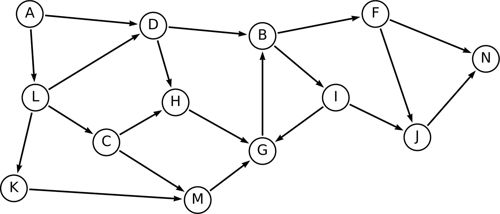
(a)

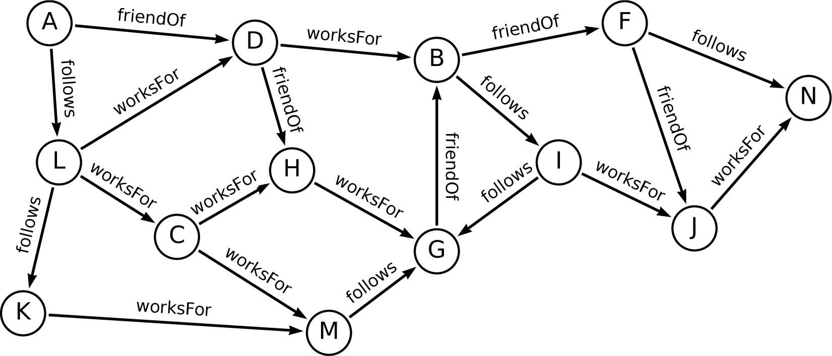
(b)

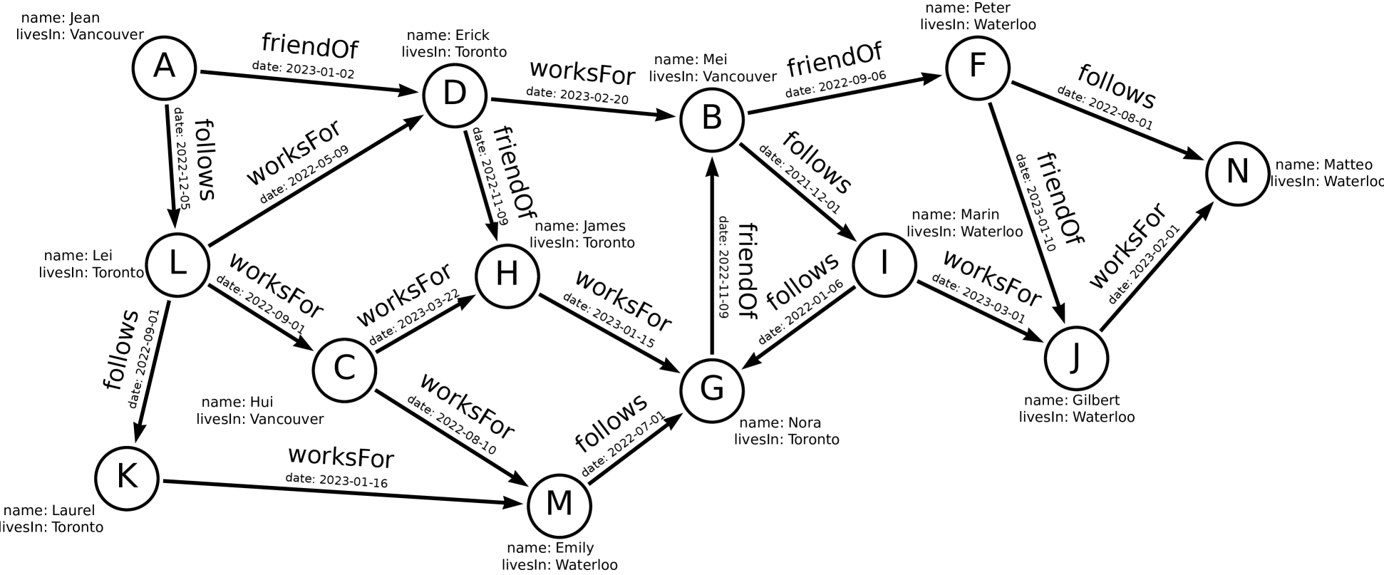
(c)

Figure 1. A plain graph (a), an edge-labeled graph (b), and a property graph (c).

2.1. The landscape of graph queries

Graph queries can be broadly categorized into two classes: pattern matching queries and navigational queries. Pattern matching queries define a query graph that is matched against the input data graph. Matching triangles is a notable instance of pattern matching. An example query is to find vertices $\{x,y,z\}$ in the edge-labeled graph in Fig. 1 such that the following patterns can be satisfied: $(x,\texttt{follows},y)$, $(x,\texttt{follows},z)$, and $(y,\texttt{worksFor},z)$. $\{A,L,D\}$ is a triple of such vertices in Fig. 1. Navigational queries define a mechanism (usually a regular expression) that will be used to guide the navigation in the input graph. An example of navigational query is to find all the direct and indirect friends of person $A$ in Fig. 1(b), where the query searches for friends of $A$ and also the friends of the friends of $A$, and so on. Navigational queries are clearly more expressive than pattern matching queries as they include recursion. We note that both pattern matching and navigational queries can be defined on plain graphs, edge-labeled graphs, and property graphs. Reachability queries are subclasses of navigational queries that will be elaborated on. We refer readers to the recent survey (Bonifati et al., 2018) on graph query languages.

Since this survey is on reachability indexes, we focus on navigational queries. The most notable navigational queries are regular path queries (Abiteboul and Vianu, 1997; Angles et al., 2017) on edge-labeled graphs. Such queries inspect the input graph to retrieve paths of arbitrary length between two vertices, and the visited paths should satisfy the constraints specified by regular expressions based on edge labels. Regular path queries are a subclass of path queries, and path queries can have more complex path constraints, e.g., checking the relationships between the sequences of edge labels in paths (Barceló et al., 2012). We note that there are a few additional types of navigational queries, e.g., where the navigation is through repeated trees or graph patterns (Bonifati et al., 2018). In addition, it is also possible to combine regular path queries with graph patterns to define a query graph including paths with regular expressions as path constraints, which is known as navigational graph pattern (Angles et al., 2017).

Regular path queries can be classified according to query types and edge directions on paths (Angles et al., 2017).

• Boolean: These queries take a pair of source and target vertices and a regular expression as input and return only True or False, indicating the existence of the path between the source and the target, which can satisfy the constraint imposed by the regular expression. Boolean queries are also know as path-existence queries (Angles et al., 2017) or path-finding queries (ten Wolde et al., [n. d.]).

• Nodes: These queries take a regular expression as input and return pairs of source and target vertices such that the path between them satisfies the query constraint. If the source (or the target) vertex is fixed in the queries, only a list of target (source) vertices are returned.

• Path: These queries are similar to the node queries, but also return the full paths.

Regular path queries are usually defined on edge-labeled graphs that are directed graphs (each edge has a specific direction). Practical graph query languages such as SQL/PGQ (Deutsch et al., 2022), GQL (Deutsch et al., 2022), and openCypher (Team, 2016) allow specifying the directions of edges in paths that the queries needs to retrieve, corresponding to different types of queries. Connectivity queries (Foulds, 1992) ignore the direction of the edges in the path. Reachability queries (Yu and Cheng, 2010; Angles et al., 2017) require each edge in the path to have the same direction. Finally, in two-way queries (Calvanese et al., 2002, 2003; Bonifati and Dumbrava, 2019; Angles et al., 2017) every two contiguous edges in the path have the opposite directions. In this survey, we focus on reachability queries that return a Boolean value, which is recognized as the most fundamental type of regular path queries (Angles et al., 2017).

2.2. Plain reachability

Reachability queries in plain graphs are known as plain reachability queries. Plain reachability query $Q_{r}(s,t)$ has source vertex $s\in V$ and target vertex $t\in V$ as input arguments and checks whether there exists a path from $s$ to $t$ in $\mathcal{G}$. For instance, in Fig. 1(a), $Q_{r}(A,G)=True$ because of the path $(A,D,H,G)$.

A naive way to process plain reachability queries is to use a graph traversal method, e.g., breadth-first traversal (BFS), depth-first traversal (DFS), or bidirectional breadth-first traversal (BiBFS). Such traversal methods do not require any offline computation cost but online query processing cost might be high as the traversal can visit a large portion of the input graph. A naive form of indexing for plain reachability queries is the transitive closure (TC) (Agrawal et al., 1989), that is costly to compute and materialize. Even though the online query processing cost with a TC is negligible, it is unfeasible in practice due to high time complexity.

2.3. Path-constrained reachability

Reachability queries with path constraints in edge-labeled graphs are referred to as path-constrained reachability queries. Compared to plain reachability queries, a path-constrained reachability query $Q_{r}(s,t,\alpha)$ has an additional argument $\alpha$, which is a regular expression based on edge labels. We consider the basic regular expression in this survey. More precisely, $\alpha$ has edge labels as literal characters, and concatenation ‘$\cdot$’, alternation ‘$\cup$’, and the Kleene operators (star ‘$*$’ or plus ‘$+$’) as meta-characters. The grammar of $\alpha$ is $\alpha::=l|\alpha\cdot\alpha|\alpha\cup\alpha|\alpha^{+}|\alpha^{*}$. $Q_{r}(s,t,\alpha)$ checks not only whether there exists a path from $s$ to $t$, but also whether the path can satisfy the path constraint specified by $\alpha$, i.e., whether the sequence of edge labels in the path from $s$ to $t$ form a word in the language of the regular expression $\alpha$. For instance, path constraint $\alpha=(\texttt{friendOf}\cup\texttt{follows})^{*}$ enforces that the path from $s$ to $t$ can only contain edges of labels friendOf or follows, and $Q_{r}(A,G,\alpha)=False$ in Fig. 1(b) because every path from $A$ to $G$ must include worksFor. Path-constrained reachability queries are a subclass of regular path queries (Fan et al., 2011) in the sense that the former ones only check whether a path satisfying the path constraint exists while the latter ones can return source and target nodes of such paths.

The approaches for processing regular path queries can be used to process path-constrained reachability queries, e.g., building a finite automata according to $\alpha$ and using the finite automata to guide an online traversal for the query processing. We note that the path semantic needs to be specified for processing such queries. In practice, the arbitrary path semantic has been widely adopted, e.g., SPARQL 1.1 (Steve and Andy, 2013). Due to the presence of the Kleene operators in $\alpha$, path-constrained reachability queries are inherently recursive, which are known to be computationally expensive. Another naive approach for processing path-constrained reachability queries is precomputing an extended transitive closure, which records for any pair of vertices $(s,t)$ not only whether $t$ is reachable from $s$ but also the information related to edge labels of the paths from $s$ to $t$ for the evaluation of path constraint $\alpha$, referred to as a generalized transitive closure (GTC) (Jin et al., 2010; Zhang et al., 2023b). However, GTCs are even more expensive to compute than TCs that are already known to be computationally expensive. Thus, precomputing GTCs is not feasible in practice.

2.4. Reachability indexes

Reachability indexes are nontrivial data structures that can effectively compress the naive indexes, e.g., TCs or GTCs, and can also be efficiently computed. In addition, query processing using reachability indexes can be more efficient than the approaches based on graph traversals. The main intuition of designing reachability indexes is to strike the balance between offline and online computations for reachability query processing. According to the types of reachability queries, there exist plain reachability indexes (Agrawal et al., 1989; Jagadish, 1990; Cohen et al., 2003; Haixun Wang et al., 2006; Chen and Chen, 2008; Jin et al., 2008, 2009; Cheng et al., 2013; Jin and Wang, 2013; Chen et al., 2005; Trißl and Leser, 2007; Yildirim et al., 2010; Seufert et al., 2013; Veloso et al., 2014; Wei et al., 2014; Su et al., 2017; Zhu et al., 2014; Cai and Poon, 2010; Yano et al., 2013; Hanauer et al., 2022; Merz and Sanders, 2014; Bramandia et al., 2010; Schenkel et al., 2005; Henzinger and King, 1995; Roditty, 2013; Roditty and Zwick, 2004; Lyu et al., 2021; Yildirim et al., 2013) and path-constrained reachability indexes (Jin et al., 2010; Zou et al., 2014; Valstar et al., 2017; Peng et al., 2020; Chen and Singh, 2021; Chen et al., 2022; Zhang et al., 2023b). We further categorize plain reachability indexes and path-constrained reachability indexes in Tables 1 and 2, respectively.

3. Plain Reachability Indexes

Most of the indexes can be grouped into index classes according to the underlying classes with a few additional techniques. The three main classes are:

• Tree cover;

• 2-Hop labeling (Cohen et al., 2003);

• Approximate transitive closure (Wei et al., 2014).

These indexes can be further characterized according to $4$ metrics (Table 1):

• The index class column indicates the main class of the indexing approach: tree cover, 2-hop, approximate transitive closure, and chain cover. A few other approaches also exist, which have specific designs that are different from these main classes.

• The index type column indicates whether an indexing approach is a complete index or a partial index. The former records all the reachability information in the graph such that queries can be processed by using only index lookups, while the latter records only partial information such that query processing might need to traverse the input graph. Partial indexes can be further classified into partial indexes without false positives and partial indexes without false negatives, indicated by no FP and no FN, respectively. In the first subclass, if index lookups return $True$, query result $True$ can be immediately returned as the index does not contain false positives. Otherwise, graph traversals are needed for query processing. Techniques in the second subclass work in the opposite way, i.e., graph traversals are necessary if the index lookups return $True$.

• The input column indicates whether an indexing approach assumes a directed acyclic graph (DAG) or a general graph as input. Assuming DAGs as input is not a major issue in terms of query processing as an efficient reduction can be used (discussed later).

• The dynamic column indicates whether an indexing approach can handle dynamic graphs with updates. There exist two types of dynamic graphs: fully dynamic graphs with both edge insertions and deletions indicated by I&D, and insertion-only graphs with only edge insertions indicated by I. We note that although assuming DAG as input is not a major issue for query processing on static graphs, that assumption becomes a major bottleneck in maintaining indexes on dynamic graphs because indexing techniques designed with the DAG assumption have to deal with the problem of maintaining strongly connected components, which can be expensive.

Table 1. Overview of plain reachability indexes.

. Indexing Technique Index Class Index Type Input Dynamic Construction Time Index size Query Time Tree cover (Agrawal et al., 1989) Tree cover Complete DAG No $O(|V||E|)$ $O(|V|^{2})$ $O(\log|V|)$ Tree+SSPI (Chen et al., 2005) Tree cover Partial (no FP) DAG No $O(|E|+|V|)$ $O(|E|+|V|)$ $O(|E|-|V|)$ Dual labeling (Haixun Wang et al., 2006) Tree cover Complete DAG No $O(|V|+|E|+t^{3})$ $O(|V|+|E|+t^{2})$ $O(1)$ or $O(\log t)$ GRIPP (Trißl and Leser, 2007) Tree cover Partial (no FP) General No $O(|E|+|V|)$ $O(|E|+|V|)$ $O(|E|-|V|)$ Path-tree (Jin et al., 2008, 2011) Tree cover Complete DAG Yes (I&D) $O(k|E|)$ or $O(|V||E|)$ $O(k|V|)$ $O((\log k)^{2})$ GRAIL (Yildirim et al., 2010) Tree cover Partial (no FN) DAG No $O(k(|V|+|E|))$ $O(k|V|)$ $O(k)$ or $O(|V|+|E|)$ Ferrari (Seufert et al., 2013) Tree cover Partial (no FN) DAG No $O(k^{2}|E|)$ $O((k+|S|)|V|)$ $O(k)$ or $O(|V|+|E|)$ DAGGER (Yildirim et al., 2013) Tree cover Partial (no FN) DAG Yes (I&D) $O(k(|V|+|E|))$ $O(k|V|)$ $O(k)$ or $O(|V|+|E|)$ 2-Hop (Cohen et al., 2003) 2-Hop Complete General No $O(|V|^{4})$ $O(|V||E|^{1/2})$ $O(|E|^{1/2})$ Ralf et al. (Schenkel et al., 2005) 2-Hop Complete General Yes (I&D) - - - 3-Hop (Jin et al., 2009) 2-Hop Complete DAG No $O(k|V|^{2}|Con(\mathcal{G})|)$ $O(k|V|)$ $O(\log|V|+k)$ U2-hop (Bramandia et al., 2010) 2-Hop Complete DAG Yes (I&D) - - - Path-hop (Cai and Poon, 2010) 2-Hop Complete DAG No - - - TFL (Cheng et al., 2013) 2-Hop Complete DAG No $O(T)$ - $O(|L_{out}(s)|+|L_{in}(t)|)$ DL (Jin and Wang, 2013) 2-Hop Complete General No $O(|V|(|V|+|E|)L)$ - $O(|L_{out}(s)|+|L_{in}(t)|)$ HL (Jin and Wang, 2013) 2-Hop Complete DAG No $O(H)$ - $O(|L_{out}(s)|+|L_{in}(t)|)$ PLL (Yano et al., 2013) 2-Hop Complete General No $O(|V||E|)$ $O(|V|\log|V|)$ $O(\log|V|)$ TOL (Zhu et al., 2014) 2-Hop Complete DAG Yes (I&D) $O(\sum^{k}_{i=1}(|E_{i}|+k|V_{i}|))$ $O(\sum^{k}_{i=1}|V_{i}|)$ $O(|L_{out}(s)|+|L_{in}(t)|)$ DBL (Lyu et al., 2021) 2-Hop Partial (mixed) General Yes (I) $O((k+k^{\prime})(|V|+|E|))$ $O((k+k^{\prime})|V|)$ $O(k+k^{\prime})$ or $O((k+k^{\prime})(|V|+|E|))$ O’Reach (Hanauer et al., 2022) 2-Hop Partial (mixed) DAG No $O((d+kp)(|V|+|E|))$ $O(|V|)$ $O(k+d+1)$ or $O(|V|+|E|)$ IP (Wei et al., 2014, 2018) Approximate TC Partial (no FN) DAG Yes (I&D) $O((k+h)(|V|+|E|))$ $O((k+h)|V|)$ $O(k)$ or $O(k|V|r^{2})$ BFL (Su et al., 2017) Approximate TC Partial (no FN) DAG No $O(s(|V|+|E|))$ $O(s|V|)$ $O(s)$ or $O(s|V|+|E|)$ Chain Cover (Jagadish, 1990) Chain Cover Complete DAG Yes (I&D) $O(|V|^{3})$ $O(k|V|)$ $O(\log k)$ Optimal Chain Cover (Chen and Chen, 2008) Chain Cover Complete DAG Yes (I&D) $O(|V|^{2}+k^{3/2}|V|)$ $O(k|V|)$ $O(\log k)$ Feline (Veloso et al., 2014) - Partial (no FN) DAG No $O(|V|\log|V|+|E|)$ $O(|V|)$ $O(1)$ or $O(|V|+|E|)$ Preach (Merz and Sanders, 2014) - Partial (no FP) DAG No $O(|V|\log|V|+|E|)$ $O(|V|)$ $O(1)$ or $O(|V|+|E|)$

3.1. Tree-cover-based indexes

In the tree cover index (original paper: (Agrawal et al., 1989)), each vertex is assigned one or more intervals, and queries are processed by using intervals of the source and target vertices. The intervals are obtained based on spanning trees of the input graph, followed by specifically addressing non-tree edges. There have been a number of proposals that fall under this class (Chen et al., 2005; Haixun Wang et al., 2006; Trißl and Leser, 2007; Jin et al., 2011, 2008; Yildirim et al., 2010; Seufert et al., 2013; Yildirim et al., 2013). These sometimes differ in the computation of the vertex intervals.

3.1.1. The approach

The tree cover index is computed in three steps:

1. Transforming a general graph (potentially) with cycles to a DAG;

2. Computing spanning trees and the interval labeling over this DAG;

3. Hooking up roots of spanning trees and indexing non-tree edges.

Transformation. A general graph is transformed into a DAG by identifying all the strongly connected components (SCCs) and selecting a representative vertex in each SCC. Given a vertex $v$ that belongs to a SCC, we use $Rep(v)$ to denote the representative of $v$ in the SCC. For instance, the general graph in Fig. 1(a) can be transformed into the DAG in Fig. 3, where $Rep(G)=Rep(I)=Rep(B)=B$. After the transformation, every edge $(u,v)$ in the general graph is transformed into an edge $(Rep(u),Rep(v))$ in the resulting DAG, e.g., the edge $(H,G)$ in Fig. 1(a) is kept as the edge $(G,B)$ in Fig. 3. The transformation can be done in $O(|V|+|E|)$ time using Tarjan’s strongly connected components algorithm (Tarjan, 1972). Thus, most plain reachability indexes in the literature assume DAGs as input since generalization is trivial.

Query reduction with the transformation. With the transformation, a reachability query on the general graph can be reduced to a corresponding query on the DAG, i.e., a query $Q_{r}(s,t)$ in the general graph is reduced to a query $Q_{r}(Rep(s),Rep(t))$. The case of $Rep(s)=Rep(t)$ indicates that $s$ and $t$ belong to the same SCC, which means that $t$ is reachable from $s$. Thus, $True$ can be immediately returned as the query result. If $Rep(s)\neq Rep(t)$, then the query needs to be processed on the DAG. For example, $Q_{r}(A,I)$ on the general graph in Fig. 1 is reduced to $Q_{r}(A,B)$ that needs to be processed in the DAG in Fig. 3.

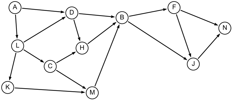
Figure 2. The DAG obtained by transforming the plain graph in Fig. 1(a)

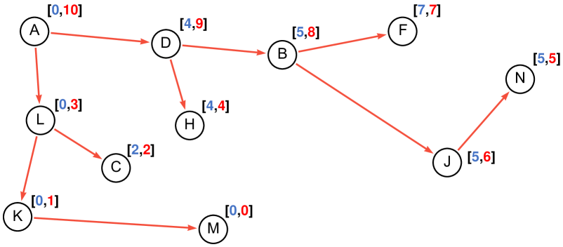
Figure 3. The spanning tree of the DAG in Fig. 3 and the interval labeling of the spanning tree.

Spanning trees and the interval labeling. To efficiently process reachability queries on the DAG, the tree cover approach first computes the spanning trees in the DAG and then computes the interval labeling according to the spanning trees. For the DAG in Fig. 3, a corresponding spanning tree is presented in Fig. 3. The interval labeling can be efficiently computed and is able to include all the reachability information in the spanning tree. Specifically, the interval labeling assigns an interval to each vertex $v$ in the tree, which is computed based on a postorder traversal from the root in the tree. Let $\mathcal{L}_{v}=[a_{v},b_{v}]$ be the interval assigned to vertex $v$. Then, the second endpoint $b_{v}$ is the postorder number of $v$, and the first endpoint $a_{v}$ is the lowest postorder number of all the descendants of $v$ in the tree. In Fig. 3, we present the intervals that are computed based on the postorder traversal from root $A$.

Query processing with the interval labeling. The vertex intervals can be used to efficiently process a reachability query $Q_{r}(s,t)$ by checking whether $b_{t}\in[a_{s},b_{s}]$. The intuition is processing $Q_{r}(s,t)$ by checking whether the subtree rooted at $s$ in the spanning tree contains $t$, and the intervals assigned to $s$ and $t$ encode sufficient information for such a checking. Consider the previous query $Q_{r}(A,B)$. The postorder number of $B$ is contained in the interval of $A$ as $8\in[0,10]$. Thus, $Q_{r}(A,B)=True$. Using the intervals, $Q_{r}(s,t)$ can also be processed by checking whether the interval of $s$ subsumes the interval of $t$, e.g., for $Q_{r}(A,B)$,$\mathcal{L}_{B}\subseteq\mathcal{L}_{A}$ as $[5,8]\subseteq[0,10]$. These two approaches are essentially equivalent.

Two major problems arise with this approach:

• In order to cover all the vertices in a graph to assign an interval to each vertex, a spanning forest might be necessary, which is a set of spanning trees.

• Interval labeling can only cover the reachability information through paths in a spanning tree.

Hooking up roots of spanning trees. The implication of the first problem is the following. If interval labeling is computed independently for each spanning tree, then the intervals cannot be used to compute reachability queries between two vertices that are in different spanning trees. To deal with this problem, a virtual root (VR) can be created, which is linked to the root of each spanning tree. This results in a unified spanning tree and the technique discussed above would then apply. Consider the DAG in Fig. 4(a). A VR is created to link $A$ and $E$ that are the roots of spanning trees.

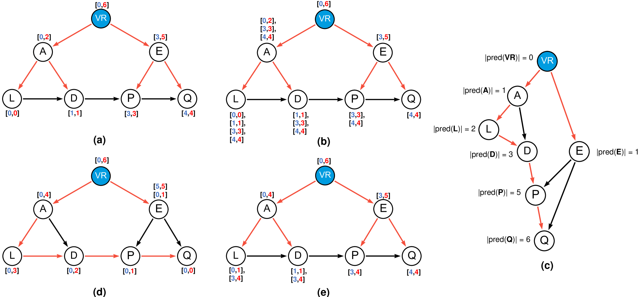
Figure 4. Examples for illustrating the tree cover index, where spanning trees are highlighted in red.

Indexing non-tree edges. The second problem implies that if a target vertex is only reachable from a source vertex via paths including non-tree edges, that reachability information is not handled in the interval labeling approach. Consider the example in Fig. 4(a), vertex $Q$ is reachable from vertex $L$, but the interval $\mathcal{L}_{L}$ does not contain the postorder number $4$ of $Q$. This issue is addressed by first computing intervals according to a spanning tree and then inheriting vertex intervals. Specifically, vertices are examined in a reverse topological order (from bottom to top), and then for each edge $(u,v)$ in the DAG, $u$ inherits all the intervals of $v$. There might be cases where, after performing the interval inheritance for all the outgoing edges of $u$, some intervals (of $u$) are subsumed by the other intervals. In this case, the subsumed intervals can simply be deleted. Fig. 4(b) shows the intervals of all the vertices after performing the interval inheritance and removing subsumed intervals according to the interval labeling on the spanning tree in Fig. 4(a).

The optimum tree cover. The spanning tree, based on which the interval labeling is computed, has an important impact on the total number of intervals of vertices in the DAG following interval inheritance. To understand this, consider the two sets of intervals computed for the same DAG but using different spanning trees in Fig. 4(b) and Fig. 4(d). Both sets of intervals are able to cover the reachability information in the DAG, but Fig. 4(d) has less intervals than Fig. 4(b). So, an important question is how to compute a spanning tree that can lead to the minimum number of intervals. The optimum tree cover (Agrawal et al., 1989) is the spanning tree such that all the reachability information in the DAG can be recorded by using the minimum number of intervals. The spanning tree highlighted in red shown in Fig. 4(c) is the optimum tree cover of the DAG, and Fig. 4(d) shows the set of intervals computed based on the optimum tree cover, which has less intervals than Fig. 4(b). The complexity of computing the minimum index based on the optimum tree cover is the same as the complexity of computing the transitive closure (Agrawal et al., 1989), which is unfeasible in practice.

Merging adjacent intervals. An optimization technique to further reduce the number of intervals is to merge adjacent intervals. Specifically, if vertex $v$ has two intervals $[a_{v},b_{v}]$ and $[a^{\prime}_{v},b^{\prime}_{v}]$ with $a^{\prime}_{v}=b_{v}+1$ , then the two intervals can be merged into the interval $[a_{v},b^{\prime}_{v}]$. This may result in overlapping intervals, i.e., $a_{v}\leq b_{v}\leq a^{\prime}_{v}\leq b^{\prime}_{v}$, and these can also be merged into $[a_{v},b^{\prime}_{v}]$. For vertex $A$ in Fig. 4(b), the intervals $[0,2],[3,3],$ and $[4,4]$ can be merged into one interval $[0,4]$, resulting in Fig. 4(e). Merging reduces the total number of intervals in Fig. 4(b) from $15$ to $9$ as shown in Fig. 4(e). We note that the effect of merging intervals is not considered in the optimum tree cover.

In essence, the tree cover index is an interval labeling approach that incorporates interval inheritance and merging. The primary limitation of the tree cover approach lies in the possibility of a substantial number of intervals.

3.1.2. Reducing the number of intervals

Several follow-up works (Chen et al., 2005; Yildirim et al., 2010; Seufert et al., 2013) aim at reducing the number of intervals for each vertex. The latest works adopt two types of designs for reducing the number of intervals:

• Recording exactly $k$ intervals for each vertex, e.g., GRAIL (Yildirim et al., 2010);

• Recording at most $k$ intervals for each vertex, e.g., Ferrari (Seufert et al., 2013).

In both approaches, $k$ is an input parameter. Neither approach computes a complete index, and the query results using index lookups may contain false positives but no false negative. These partial indexes can be used to guide online traversal to compute correct query results.

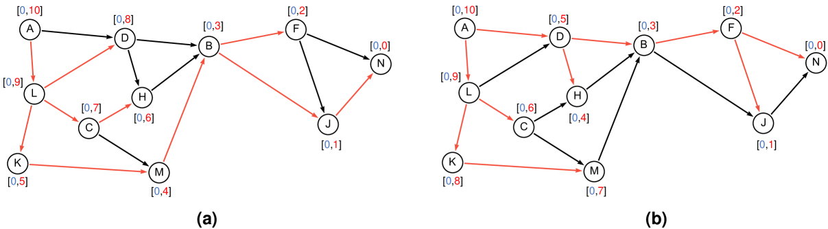
Figure 5. Running examples of GRAIL. Two intervals for each vertex in the DAG are computed based on two different spanning trees highlighted in red.

The interval labeling scheme in GRAIL. Each vertex has $k$ intervals that are computed by using $k$ random spanning trees, referred to as $\mathcal{L}_{v}=(\mathcal{L}^{1}_{v},..,\mathcal{L}^{k}_{v})$, where $\mathcal{L}^{i}_{v}=[a^{i}_{v},b^{i}_{v}]$ is the interval of $v$ computed based on the $i$-th spanning tree. Similar to the interval labeling in the tree cover approach, $\mathcal{L}^{i}_{v}$ is computed based on a postorder traversal of the spanning tree, and $b^{i}_{v}$ records the postorder number of $v$ in the tree. However, the computation of $a^{i}_{v}$ is different from the computation in the tree cover approach. Specifically, for each vertex $v$, GRAIL gets the minimum first endpoint of all the outgoing neighbours of $v$ in the DAG, denoted as $c$, and then records the minimum of $c$ and $b^{i}_{v}$ as $a^{i}_{v}$, i.e., $a^{i}_{v}=min(c,b^{i}_{v}),c=min\{a^{i}_{u}:u\in outNei(v)\}$, where $outNei(v)$ is the set of outgoing neighbours of $v$ in the DAG. Consider the DAG in Fig. 5(a), where a spanning tree is computed and highlighted in red, and the interval of each vertex is computed according to the schema in GRAIL. For vertex $B$, the outgoing neighbours of $B$ include vertices $F$ and $J$, of which the minimum first endpoint is $0$ that is smaller than the postorder number of $B$. Thus, the first endpoint in the interval of $B$ is $0$. The interval labeling schema of GRAIL allows to directly compute the intervals on the DAG without the need of inheriting intervals.

Query processing in GRAIL. Query processing with the intervals in GRAIL does not have false negatives but may have false positives. Consider query $Q_{r}(K,C)$ on the intervals computed in Fig. 5. The interval of $C$ is not subsumed by the interval of $K$. Therefore, the answer provided by the intervals is False. Indeed, $C$ is not reachable from $K$ in the DAG. However, for query $Q_{r}(D,M)$, the interval of $M$ is subsumed by the interval of $D$. Thus, the answer provided by the intervals is True, which does not correspond to the reachability information in the DAG as $M$ is not reachable from $D$. This is an example of false positive answer.

Guided DFS in GRAIL. To avoid false positive answer to a query $Q_{r}(s,t)$, a graph traversal is needed when the interval of $s$ subsumes the interval of $t$. The graph traversal, which is usually a DFS from $s$, can be guided by leveraging the partial index. Specifically, when the DFS visits vertex $v$, the intervals of $v$ and $t$ can be used to check whether or not $t$ is reachable from $v$, which can be correctly processed by using the intervals. If so, $v$ can be pruned in the DFS. Consider query $Q_{r}(D,M)$ in the intervals computed in Fig. 5. The DFS is performed from vertex $D$, and then for each outgoing neighbour $v$ of $D$, we check whether $D$ is reachable from $v$ using the intervals. The outgoing neighbour $B$ cannot reach the target $M$ as the interval of $B$ does not subsume the interval of $M$. Then, $B$ is pruned in this DFS. For outgoing neighbour $H$, there might be false positives with the intervals. Then, $H$ is further explored by the DFS. Since $B$, the the outgoing neighbour of $H$, cannot reach $M$. Therefore, the DFS terminates and returns False as the query result.

Reducing the possibility of having false positives in GRAIL. To reduce the possibility of false positives, GRAIL computes $k$ intervals using $k$ random spanning trees. Consequently, each vertex has $k$ intervals, i.e., $\mathcal{L}_{v}=(\mathcal{L}^{1}_{v},..,\mathcal{L}^{k}_{v})$. With the $k$ intervals, the interval of $s$ subsumes the interval of $t$ if and only if $\mathcal{L}^{i}_{s}$ subsumes $\mathcal{L}^{i}_{t}$ for each $i\in(1,...,k)$. Note that the interval subsumption is checked on the intervals of $s$ and $t$ that are computed on the same spanning tree. Consider the running example in Fig. 5, where two spanning trees are computed on the same DAG, which give two intervals for each vertex. For query $Q_{r}(D,M)$, with intervals of $D$ and $M$ computed based on the second spanning tree shown in Fig. 5(b), the interval of $D$ does not subsume the interval of $M$. Therefore, query result is False. We note that the topological ordering of the DAG can be used to further reduce the possibility of having false positives. Eventually, false positives are still possible in the query processing with $k$ intervals. Thus, the guided DFS is still necessary.

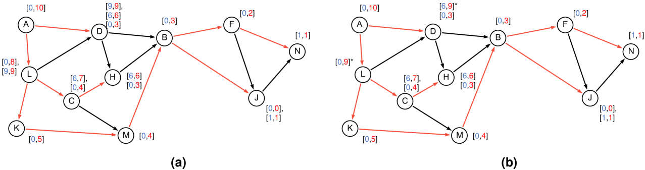
Figure 6. Running examples of Ferrari. Each vertex in (b) has at most $k$ intervals obtained by merging non-adjacent intervals in (a).

The interval labeling scheme in Ferrari. Ferrari adopts a different design to reduce the number of intervals. The overall computations in Ferrari follow the steps in the tree cover approach, i.e., computing intervals based on spanning trees, followed by inheriting and merging intervals. The adjacent intervals, e.g., the intervals $[0,0]$ and $[1,2]$, can be merged into $[0,2]$. This is termed merging without gaps. Ferrari also merges non-adjacent intervals to get approximate intervals. This is termed merging with gaps, and does not exist in the original tree cover proposal. Merging with gaps can be applied recursively such that each vertex has $k$ intervals. Consider the example in Fig. 6, where intervals of each vertex in Fig. 6(a) are merged so that each vertex has at most $2$ intervals (Fig. 6(b)). Vertex $D$ in Fig. 6(a) has $3$ intervals, which is merged into $2$. Two options are available: (i) merging the first two intervals $[0,3]$ and $[6,6]$ into $[0,6]^{*}$ (starred intervals denote approximate ones); (ii) merging the last two intervals $[6,6]$ and $[9,9]$ into $[6,9]^{*}$. In this example, option (ii) is adopted as the size of the corresponding approximated interval is smaller – the intuition is to add less error when merging non-adjacent intervals. When non-adjacent intervals are merged, reachability information that does not exist in the graphs is added into the intervals. Since the primary goal of Ferrari is to reduce the number of intervals, the merging options that introduce less error are preferable.

Query processing in Ferrari. Query processing in Ferrari first uses exact intervals to find reachability. If that is not possible, approximate intervals are used. As in GRAIL, using exact intervals may result in false negatives (but no false positives). Using approximate intervals may result in false positives but no false negatives, because approximated intervals are obtained only by merging non-adjacent intervals. In query $Q_{r}(D,N)$ of Fig. 6(b), the postorder number of $N$ is contained in the exact interval of $D$, thus the answer is True. For query $Q_{r}(D,K)$ in Fig. 6(b), we can not determine the query result with the exact interval of $D$ as it does not contain the postorder number of $K$. In this case, the approximate interval $[6,9]^{*}$ of $D$ is used, resulting in the answer False, since the postorder number is not contained in $[6,9]^{*}$. As false positives are still a possibility, graph traversal is still needed as in GRAIL.

Although partial indexes require additional graph traversals for query processing, their index building time and index size scale linearly with the input graph size, making them one of the first methods feasible for large graphs with millions of vertices. In addition, reachability processing using these indexes can be an order of magnitude faster than graph traversals.

Other approaches for non-tree edges. There also exist a few early approaches that are designed to deal with the problem of non-tree edges in the interval labeling technique, including Tree-SSPI (Chen et al., 2005), Dual-labeling (Haixun Wang et al., 2006), and GRIPP (Trißl and Leser, 2007). These early indexes have specific designs that are different from the ones in GRAIL and Ferrari. We briefly discuss them below.
Tree-SSPI (Chen et al., 2005) distinguishes two kinds of paths in a DAG: tree paths of only tree edges, and remaining paths of non-tree edges. A target vertex $t$ is reachable from a source vertex $s$ via one of these, and the former case can be simply addressed by interval labeling. For remaining paths, additional information is kept about the predecessors of the target vertex that is used for answering the query.
Dual-labeling (Haixun Wang et al., 2006) also leverages the interval labeling technique to deal with reachability caused by tree paths. The interval $[v_{a},v_{b})$ is kept for each vertex $v$, where $v_{a}$ and $v_{b}-1$ are the preorder and postorder numbers of $v$ respectively (this is equivalent to the original one as $Q_{r}(s,t)$ can be simply processed by checking whether $t_{a}$ is in the range of $[s_{a},s_{b})$). Dual-labeling records a link table to process reachability caused by paths of non-tree edges. Specifically, if there is a non-tree edge $(u,v)$ such that $v$ is not reachable from $u$ via tree paths, the link $u_{a}\rightarrow[v_{a},v_{b})$ is recorded in the link table. Then, in the link table, if two links $u_{a}\rightarrow[v_{a},v_{b})$ and $x_{a}\rightarrow[y_{a},y_{b})$ satisfy the condition that $x_{a}$ is in the range of $[v_{a},v_{b})$, an additional link $u_{a}\rightarrow[y_{a},y_{b})$ is recorded in the link table as well, i.e., computing and storing the transitive closure of the link table. Given a query $Q_{r}(s,t)$ that cannot be processed by the intervals of $s$ and $t$, dual-labeling looks for a link $u_{a}\rightarrow[v_{a},v_{b})$ such that $u_{a}$ is in the range of $[s_{a},s_{b})$ and $t_{a}$ is in the range of $[v_{a},v_{b})$.
GRIPP (Trißl and Leser, 2007) performs a DFS and directly computes intervals of vertices on a general graph that can have cycles. As the incoming degree of a vertex $v$ in the graph can be $k>1$, $v$ will be considered having $k$ instances in GRIPP. One of the $k$ instances is treated as the tree instance of $v$, denoted as $v^{\prime}$. During the DFS, the outgoing neighbours of tree instances will be visited while the search will not be expanded for the case of non-tree instances. For processing $Q_{r}(s,t)$, GRIPP uses the interval of the tree instance $s^{\prime}$ to retrieve a set of vertex instances that are reachable from $s^{\prime}$, denoted as reachable instance set (RIS) of $s$ or $RIS(s)$. If any instance of $t$ is in $RIS(s)$, query result $True$ is immediately returned. Otherwise, the non-tree instances in $RIS(s)$ are retrieved to check reachability. This procedure is performed recursively until none instance of $t$ is reached, and in this case query result $False$ is returned.

3.1.3. Advanced covers

The tree-cover-based approaches use spanning trees to cover an input DAG and computes the interval labeling on the spanning trees. Path-tree labeling uses a structure that is more advanced than a tree in the input DAG, instead of spanning trees. The approach first computes a disjoint set of paths in the graph such that each vertex belongs to a specific path. Each of these sets of paths is known as a path partition. Then, the advanced structure is computed by partitioning the DAG by the path partition to obtain a path-tree graph, where each vertex represents a path in the DAG. The interval labeling with additional information is computed on the spanning trees of the path-tree graph. The main reason of adopting the advanced cover is that the number of non-covered edges is smaller than that based on a tree cover. The number of non-covered edges has an impact on the index size. Thus, the advanced cover can lead to an index of smaller size. The advanced structure provides more comprehensive coverage of the DAG compared to the spanning tree because: (i) an edge in a path of the path partition is considered covered; (ii) a pair of crossed edges from one path to another path in the path partition contains redundancy and keeping one of two edges is sufficient. To understand the second fact, consider paths $p_{1}$ and $p_{2}$, and edges $(v_{2},u_{1})$ and $(u_{2},v_{1})$, where $u_{1}$ and $v_{1}$ are vertices in $p_{1}$ and $v_{1}$ is reachable from $u_{1}$, and $u_{2}$ and $v_{2}$ are vertices in $p_{2}$ and $v_{2}$ is reachable from $u_{2}$. In this case, $(u_{2},v_{1})$ is redundant because $u_{2}$ can reach $v_{2}$, $v_{2}$ can reach $u_{1}$, and $u_{1}$ can reach $v_{1}$. The reachability in the path-tree graph can be processed by computing the interval labeling augmented with additional information of vertices in paths, i.e., computing whether the path of the source can reach the path of the target in the path-tree graph, followed by checking the positions of the vertices in each path. Reachability caused by non-covered edges is handled by computing the corresponding transitive closure, which is basically the approach used in dual-labeling (Haixun Wang et al., 2006).

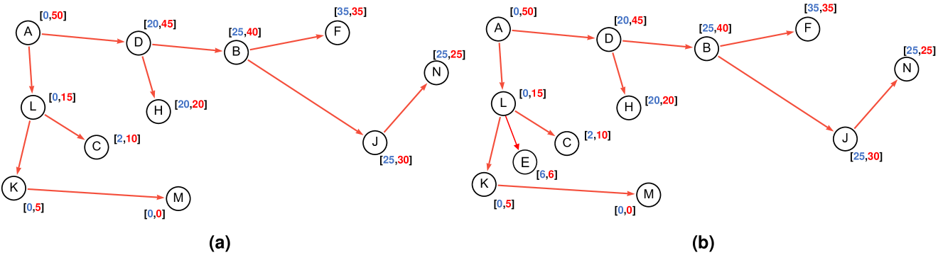
Figure 7. The interval labeling computed by using the non-contiguous postorder numbers.

3.1.4. Techniques for maintaining intervals on dynamic graphs

A few tree-cover-based approaches also address index maintenance as the graph is updated. Due to their reliance on a DAG, tree-cover-based approaches need to maintain two kinds of reachability information: reachability within SCCs and reachability within DAGs. Maintaining SCCs over dynamic graphs is expensive, as edge insertions or deletions might lead to merging or splitting SCCs, requiring recomputing SCCs in the worst case. For maintaining the second kind of reachability information, a few optimization techniques have been adopted in existing solutions, discussed below.

Non-contiguous postorder numbers. In the original tree cover index, the postorder numbers computed for each vertex do not need to be contiguous. The intervals in Fig. 3 are computed based on the contiguous postorder numbers $(0,1,2,3,4,5,6,7,8,9,10)$. If the contiguous sequence is replaced with the following non-contiguous sequence $(0,5,10,15,20,25,30,35,40,45,50)$, the corresponding intervals are still correct (Fig. 7(a)). The benefit of using a non-contiguous sequence is that the gaps between the non-contiguous postorder numbers can be used to deal with tree-edge insertions. In Fig. 7, where tree-edge $(L,E)$ is inserted into the tree in Fig. 7(a), the gap between the postorder numbers of $K$ and $C$ can be leveraged to get the postorder number of $E$ ($6$ in this example), based on which the interval $[6,6]$ of $E$ can be computed. The intervals for the other vertices remain unchanged. If there is no gap between non-contiguous postorder numbers, then recomputing the postorder numbers is necessary. Determining a reasonable gap between non-contiguous postorder numbers for real-world applications has not been studied.

Edge deletions in partial indexes allowing false positives. Dagger (Yildirim et al., 2013) is an extension of GRAIL to dynamic graphs, so it is a partial index without false negatives in the query result but may have false positives. It also leverages the non-contiguous postorder numbers to deal with tree edge insertions. The main issue addressed in Dagger is that when an edge in the DAG is deleted, the index does not require any updates. The reason is that deleting edges only introduces false positives in the index that are allowed in Dagger.

3.1.5. Chain-cover indexes

Chain cover (Jagadish, 1990) index class is similar to the tree cover index class as both of them use structures to cover the input graph, which are chains in the former and trees in the latter. Tree cover can be thought of as a variant of chain cover (Jagadish, 1990). Tree cover can provide a better compression rate than chain cover (Jin et al., 2011) because each vertex in a chain has no more than one immediate successor while each vertex in a tree has multiple immediate successors, which leads to the difference in compression rates. In addition, recent indexes are designed based on tree cover. For all the above reasons, we will not further elaborate on chain cover in this survey.

3.2. 2-hop-based indexes

Given two paths $(s,u)$ and $(u,t)$, the existence of the path $(s,t)$ is obvious. Obtaining new paths by concatenating those with common vertices can save storage space in the transitive closure. The intuition behind the 2-hop index is to maintain paths that can be achieved via two hops, and to use path concatenation to compress transitive closures.

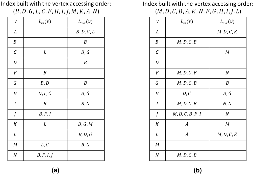
Figure 8. The 2-hop indexes built for the graph in Fig. 1(a). Both indexes can fully record the reachability information. Note that the index shown in (a) has a smaller size than the index shown in (b).

3.2.1. The approach

In the 2-hop index (or the 2-hop labeling), each vertex $v\in V$ is labeled with two sets of vertices $L_{in}(v)$ and $L_{out}(v)$, such that the following two conditions are satisfied: (i) $L_{in}(v),L_{out}(v)\subseteq V$, and there is a path in $G$ from every $x\in L_{in}(v)$ to $v$ and there is a path in $G$ from $v$ to every $x\in L_{out}(v)$; (ii) for any two vertices $s,t\in V$, $t$ is reachable from $s$ if and only if $L_{out}(s)\cap L_{in}(t)\neq\emptyset$. Notice that the 2-hop index assumes that $v$ is included in $L_{in}(v)$ and $L_{out}(v)$ for each $v$. Without the above assumption, condition (ii) is equivalent to: $t$ is reachable from $s$ if and only if $t\in L_{out}(s)$, $s\in L_{in}(t)$ or $L_{out}(s)\cap L_{in}(t)\neq\emptyset$. Consider the index in Fig. 8(a) and query $Q(A,N)$. Since $L_{out}(A)\cap L_{in}(N)\neq\emptyset$, $Q(A,N)=True$.

In the construction of the 2-hop index, the transformation from a general graph to a DAG is optional.

3.2.2. The minimum 2-hop index

The size of the 2-hop index is $\sum_{i=1}^{n}|L_{out}(v_{i})|+|L_{in}(v_{i})|$ for a graph with $n$ vertices. Given an input graph, many 2-hop indexes can be built, such that each of them can satisfy the two conditions discussed above. The minimum 2-hop index is the one that has the smallest index size. Obviously, the minimum 2-hop index can maximumly compress the transitive closure of the input graph. We use the following toy example to explain the intuition. Consider a graph with two edges $(s,u)$ and $(u,t)$. One possible 2-hop index is to have $u$ in both $L_{out}(s)$ and $L_{in}(t)$. Another option is to record $s$ in $L_{in}(u)$ and $L_{in}(t)$ and to record $t$ in $L_{out}(u)$. The first option is preferable since it has fewer number of index entries. The general goal of building the minimum 2-hop index is to maximumly compress the transitive closure. However, the problem of computing the minimum 2-hop index is NP-hard (Cohen et al., 2003). Efficient heuristics have been proposed to reduce the index size of the 2-hop index, e.g., TFL (Cheng et al., 2013), DL (Jin and Wang, 2013), PLL (Yano et al., 2013), and TOL (Zhu et al., 2014). We take PLL as a representative to discuss the 2-hop indexing, followed by the discussion of the differences between different approaches.

The PLL indexing algorithm. The indexing algorithm of PLL consists of three major steps: (i) computing a vertex accessing order; (ii) processing vertices iteratively according to the vertex accessing order; (iii) applying pruning rules during the processing of each vertex. For computing a vertex accessing order, a simple strategy is to sort vertices according to vertex degree, i.e., $(d_{in}(v)+1)\times(d_{out}(v)+1)$, where $d_{in}(v)$ and $d_{out}(v)$ are in-degree and out-degree of each vertex $v$. Vertices are then iteratively processed according to the vertex accessing order, and processing each vertex $v$ consists of performing backward and forward BFSs from $v$ to compute $L_{out}$-entries and $L_{in}$-entries. During each BFS, PLL prunes the search space guided by a set of rules. Consider the case of forward BFS (backward BFS works similarly). When the forward BFS from $v$ visits $u$ and $u$ has been processed, i.e., $u$ ranks in front of $v$ in the vertex accessing order, $u$ is pruned in the BFS. The reason is that the reachability information due to the paths from $v$ to any vertex via $u$ has been recorded in the backward and forward BFSs performed from $u$.

Consider the graph in Fig. 1(a) to build the index in Fig. 8(a). In this example, the vertex accessing order is $(B,D,G,L,C,F,H,I,J,M,K,A,N)$, computed according to vertex degree. Then, the vertices are processed one by one according to this order starting with $B$. During the processing of $B$, the backward BFS from $B$ visits vertices $\{A,V,C,D,G,H,I,K,L,M\}$ and adds $B$ into each of their $L_{out}$. Then, the forward BFS from $B$ visits vertices $\{F,G,I,J,N\}$ and adds $B$ into the $L_{out}$ of each of them. Once $B$ is processed, the indexing algorithm starts processing $D$. The backward and forward BFS from $D$ work in a similar way. During the forward BFS from $D$, pruning is possible: although $B$ can be visited by BFS, $B$ has already been processed. Thus, $B$ can be pruned. For instance, in Fig. 1(a), $N$ is reachable from $D$ via $B$. Although $B$ is pruned in the forward BFS from $D$, the reachability information of $N$ is recorded by the index entries $B\in L_{out}(D)$ and $B\in L_{in}(N)$. The final index is presented in Fig. 8(a).

Given the vertex accessing order $(B,D,G,L,C,F,H,I,J,M,K,A,N)$, Fig. 8(a) shows the index built according to the order, whose size is $39$. However, the size of the index in Fig. 8(b) that is built according to the order $(M,D,C,B,A,K,N,F,G,H,I,J,L)$ is $47$. In general, finding the optimal order that can lead to the minimum index size is NP-hard (Weller, 2014). The vertex accessing order based on vertex degree that is used in Fig. 8(a) is an example of efficient heuristic (Yano et al., 2013).

Query optimization based on vertex accessing order. Query processing using the 2-hop index needs to check whether one of the following condition can be satisfied: $t\in L_{out}(s)$, $s\in L_{in}(t)$, or $L_{out}(s)\cap L_{in}(t)\neq\emptyset$. In order to efficiently perform the search in $L_{out}(s)$ and $L_{in}(t)$, the access order of vertices in $L_{out}(s)$ and $L_{in}(t)$ can be leveraged. This is feasible because vertices are added into $L_{out}$-entries and $L_{in}$-entries according to the vertex accessing order. Let $rank(v)$ be the vertex accessing order of $v$, and $rank(L_{out}(v))=\{rank(u)|u\in L_{out}(v)\}$ and $rank(L_{in}(v))=\{rank(w)|w\in L_{in}(v)\}$. Then, we can actually store $rank(L_{out}(v))$ and $rank(L_{in}(v))$ instead of $L_{out}(v)$ and $L_{in}(v)$, and the elements in $rank(L_{out}(v))$ and $rank(L_{in}(v))$ are naturally sorted. Given a query $Q_{r}(s,t)$, the search in $rank(L_{out}(s))$ and $rank(L_{in}(t))$ is performed. Checking whether $t\in L_{out}(s)$ or $s\in L_{in}(t)$ can be processed by the binary search of $rank(t)\in rank(L_{out}(s))$ or $rank(s)\in rank(L_{in}(t))$. In order to check whether $L_{out}(s)\cap L_{in}(t)\neq\emptyset$, merge-join can be performed without the need for sorting.

Consider the index in Fig. 8(a), where $rank(B)=1$, $rank(D)=2$, and so forth. Then, the vertices in each $L_{out}(v)$ and $L_{in}(v)$ are sorted according to their rank values, e.g., for $L_{out}(A)=\{B,D,G,L\}$ and $L_{in}(N)=\{B,F,I,J\}$, we have $rank(L_{out}(A))=\{1,2,3,4\}$ and $rank(L_{in}(N))=\{1,6,8,9\}$. To process query $Q_{r}(A,N)$, merge-join over $rank(L_{out}(A))$ and $rank(L_{in}(N))$ can be performed.

The TOL indexing framework. TOL is a general index class that generalizes the indexing algorithm of PLL. TOL computes a total order of vertices and then iteratively processes vertices to compute $L_{out}$-entries and $L_{in}$-entries according to the total order, performing pruning during processing. The vertex accessing order computed based on vertex degree is an instantiation of the total order, which is the strategy used in DL and PLL. Another instantiation is the topological folding numbers, which are computed based on a topological ordering of a DAG (obtained by applying the transformation), which is used in TFL (Cheng et al., 2013). An advanced instantiation of the total order introduced in TOL is based on the contribution score of vertices, which is defined according to the number of the vertices that can reach $v$ and the number of the vertices that are reachable from $v$. The contribution score can be approximated by a linear scan of the DAG. The TOL index built according to approximate contribution scores exhibits superior performance in terms of index construction time over those built based on previous heuristics. In addition, it can support graph updates. Among existing heuristics, only the simple strategy based on vertex degree can be applied to the case of general graphs, while other strategies require DAG as input.

3.2.3. Partial 2-hop indexes

The 2-hop indexes presented previously are complete indexes in that they record complete reachability information. Partial 2-hop indexes are also possible (e.g., DBL (Lyu et al., 2021) and O’Reach (Hanauer et al., 2022)) where the index is built only for a selected subset of vertices in the graph. In DBL, the subset of vertices are selected as those in the top-$k$ degree ranking, aka landmark vertices. In O’Reach, the subset of vertices are those residing in the middle of a topological ordering, referred as supportive vertices. Query processing in DBL and O’Reach might require graph traversals. DBL also adds BFL that is a partial index without false negatives (presented later in Section 3.3) to prune the search space when traversing the graph.

3.2.4. Extended hop-based indexes

A few indexes in the literature extends the 2-hop index. With the 2-hop index, query $Q_{r}(s,t)$ is processed by checking whether there are common vertices in $L_{out}(s)$ and $L_{in}(t)$. Some algorithms extend the definition of “common vertices” by replacing them with common chains (the 3-hop index (Jin et al., 2009)) or common trees (the path-hop index (Cai and Poon, 2010)). Although these indexes are able to further compress transitive closure, the corresponding indexing cost is higher than that of the 2-hop index, which makes them less applicable.

3.2.5. 2-hop indexes on dynamic graphs

A few 2-hop indexes can support dynamic graphs, including TOL and DBL. TOL assumes a DAG as input, which means that a general graph is first transformed into a DAG. Thus, maintaining SCCs is necessary for the index updates. TOL relies on existing approaches (Yildirim et al., 2013; Yang et al., 2019; Hanauer et al., 2020) to deal with the problem of maintaining SCCs and designs an incremental algorithm to perform index updates. The algorithm can support both edge insertions and deletions. We use the case of edge insertion to discuss the underlying intuition. Consider inserting an edge $(u,v)$ into a graph. Let $in(u)$ be the set of vertices that can reach $u$ and $out(v)$ be the set of vertices that are reachable from $v$. After inserting $(u,v)$, every vertex in $out(v)$ is reachable from every vertex in $in(u)$, and this reachability information needs to be recorded in the index. TOL computes $in(u)$ and $out(v)$ by using the snapshot of the index that exists before inserting $(u,v)$. In general, $out(v)$ is computed by using $L_{out}(v)$ and $W=\{w|\exists x\in L_{out}(v),w\text{ is reachable from }x\}$. $W$ can be efficiently computed by recording inverted index entries for each vertex, i.e., if $x\in L_{in}(w)$, then TOL records $w\in L^{-1}_{in}(x)$. The inserted index entries can make some of the index entries that exist prior to the edge insertion redundant, and such redundancy can be addressed by the TOL indexing algorithm efficiently. The case edge deletion works in a similar way in TOL. DBL can only support edge insertions, but does not assume a DAG as input, so there is no need to maintain SCCs. In DBL, $in(u)$ and $out(v)$ are computed by performing backward and forward BFSs, respectively. Early works also discussed how to maintain the 2-hop index on dynamic graphs, including the U2-hop index (Bramandia et al., 2010) and the index proposed by Ralf et al. (Schenkel et al., 2005). However, it has been shown that they cannot scale to large graphs (Zhu et al., 2014).

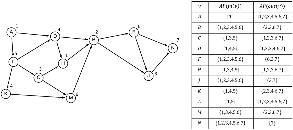
Figure 9. The BFL index built for the graph in Fig. 3.

3.3. Approximate transitive closures

3.3.1. The approach

Note the following: If vertex $u$ can reach vertex $v$, then $out(v)\subseteq out(u)$, because there might exist a vertex $w$ such that $w$ is reachable from $u$ but $w$ is not reachable from $v$. For example, in Fig. 3, $C$ can reach $B$, such that $out(B)\subseteq out(C)$. Based on the observation, we can have the following condition: if $out(v)\nsubseteq out(u)$, then $u$ cannot reach $v$. Similarly, if $in(u)\nsubseteq in(v)$, then $u$ cannot reach $v$. The two conditions are not usable for designing a reachability index as computing $out(v)$ or $in(v)$ for each vertex $v$ is equivalent to computing the transitive closure, which is unrealistic in practice. This is the basis of approximate transitive closure algorithms. The primary goal is to compute an approximate version of $out(v)$ and $in(v)$, such that they can be efficiently computed and also have a much smaller size. We use $AP()$ to denote the approximating function. The main problem is how to design $AP()$. It should satisfy the following condition: if $AP(out(v))\nsubseteq AP(out(u))$ then $out(v)\nsubseteq out(u)$. Therefore, we can derive that $u$ cannot reach $v$. Consequently, the approximate transitive closure will not have false negatives in the query results.

3.3.2. The design of the AP() function

Two approximate functions have been proposed. The first one is based on the $k$-min-wise independent permutation (IP index (Wei et al., 2014, 2018)). The approximate function computes and records in $out(v)$ and $in(v)$ the $k$ smallest numbers obtained by a permutation of vertices. The second is based on Bloom filter (BFL index (Su et al., 2017)). The approximate function computes and records in $out(v)$ and $in(v)$ the hash codes of vertices. Consequently, both indexes are partial indexes, and the query processing will not have false negatives but may have false positives as the indexes are designed based on the condition discussed previously. Thus, if the index lookup returns True, graph traversal is necessary. In this case, the guided DFS designed for GRAIL can also be applied, i.e., pruning the search space by leveraging the fact that index lookups do not provide false negatives.

We use a toy example to illustrate BFL. We compute a hash code for each vertex in the DAG in Fig. 3, and the resulting DAG and the corresponding BFL index are shown in Fig. 9, where $AP(out(v))$ and $AP(in(v))$ record the hash codes of vertices, instead of vertex identifiers. Consider the query $Q_{r}(B,C)$. Since $out(C)\nsubseteq out(B)$, we can determine that $C$ is not reachable from $B$. For the query $Q_{r}(D,M)$, index scan shows $out(M)\subseteq out(D)$ and $in(D)\subseteq in(M)$. Therefore, the query result cannot be determined by using only index lookups as there might be false positives. In this case, the guided DFS from $D$ needs to be performed. The DFS can be accelerated by leveraging the partial index to prune search space, i.e., none of the outgoing neighbours of $D$ can reach $M$, thus the query result $False$ can be immediately returned.

3.4. Other techniques

A few other indexing techniques have also been proposed that do not fall into the three main classes discussed above. We briefly discuss these techniques below.

3.4.1. Dominance drawing

Feline (Veloso et al., 2014) is designed based on dominance drawing, i.e., assigning coordinates $(v_{x},v_{y})$ to every vertex $v$ in the graph. In Feline, the assigned coordinates satisfy the following attributes: if $v$ is reachable from $u$, then $u_{x}\leq v_{x}$ and $u_{y}\leq v_{y}$. Consequently, Feline is a partial index, and the query results with index lookups computed based on the coordinates do not have false negatives but may have false positives, requiring graph traversal.

3.4.2. Reachability contraction hierarchies

Preach (Merz and Sanders, 2014) is designed based on reachability contraction hierarchies. Vertices with out-degree of $0$ (sink vertices) and those with in-degree of $0$ (source vertices) are recursively removed from the graph. This produces a vertex ordering that will be used in answering query $Q_{r}(s,t)$. The idea is to use the vertex ordering to prune the search space during the graph traversal for answering $Q_{r}(s,t)$. Specifically, queries are processed by bidirectional search from $s$ and $t$, where only paths of increasing vertex orderings are visited. Preach is essentially a partial index without false positives, and the bidirectional searches needs to be exhausted to return False, where pruning rules are designed to accelerate the searching.

3.4.3. Reachability-specific graph reduction

A few graph reduction techniques are proposed to accelerate reachability indexing, including SCARAB (Jin et al., 2012), ER (Zhou et al., 2017), and RCN (Zhou et al., 2023). The main idea is to reduce the size of the input graph by removing vertices/edges while preserving the reachability information. For instance, given a vertex $u$, if the interval labeling approach can capture both the reachability from every vertex that can reach $u$ to $u$ and the reachability from $u$ to every vertex that is reachable from $u$, then vertex $u$ can be safely removed. The reduced graph will be taken as input for building reachability indexes. These reduction techniques are orthogonal to the indexing techniques.

3.4.4. Index-free approaches

Recent works propose advanced traversal approaches for plain reachability query processing without using indexes (arrow (Sengupta et al., 2019), IFCA (Yue et al., 2023)). These approaches provide optimized traversal algorithms that are slightly faster than the naive traversal. However, query performance of these approaches is still not comparable with indexing methods as index-free methods do not leverage any offline computation.

3.5. Complexity

The complexities of plain reachability indexes are presented in Table 1. We briefly present the complexities and refer readers to each approach for detailed analysis.

Tree cover (Agrawal et al., 1989) has high complexity in index construction time due to the computation of minimum index. In dual labeling (Haixun Wang et al., 2006), $t$ is the number of non-tree edges. In path-tree (Jin et al., 2008, 2011), the number of disjoint paths in the path partition is denoted as $k$. The other approaches based on tree cover are partial indexes, which have the linear complexity with input parameter $k$ that is the number of spanning trees in GRAIL (Yildirim et al., 2010) and DAGGER (Yildirim et al., 2013), and the number of intervals in Ferrari (Seufert et al., 2013) respectively. Ferrari has an additional parameter $S$, which is a set of high-degree vertices.

2-hop labeling (Cohen et al., 2003) has high construction time. The indexing techniques are proposed to reduce the index sizes of 2-hop labeling. The bounds of index size of TFL (Cheng et al., 2013), DL (Jin and Wang, 2013), HL (Jin and Wang, 2013), and TOL (Zhu et al., 2014) are unknown as they are heuristics to address the minimum 2-hop labeling problem. They have the same query time $O(|L_{out}(s)|+|L_{out}(t)|)$ because of applying merge-join. Both DBL (Lyu et al., 2021) and O’Reach (Hanauer et al., 2022) are partial indexes. The number of chains, referred to as $k$, has an impact on the complexity of 3-hop labeling (Jin et al., 2009).

Both IP (Wei et al., 2014, 2018) and BFL (Su et al., 2017) are partial indexes. In IP, $k$ is the result size in computing min-wise independent permutations, $h$ is the limited index size for a high degree vertices, and $r$ is the reachability ratio. The parameter $s$ in BFL is the size of Bloom filter.

For the approaches based on chain cover, $k$ is the minimal number of chains. Both Feline (Veloso et al., 2014) and Preach (Merz and Sanders, 2014) are partial indexes, and they have linear construction time, index size, and $O(1)$ or $O(|V|+|E|)$ query time.

4. Path-Constrained Reachability Indexes

Compared to plain reachability queries, the main difference in path-constrained reachability queries is that these have a path constraint that is defined by a regular expression $\alpha$. In this survey, we consider the basic regular expressions, where we have edge labels as literal characters and concatenation, alternation, and the Kleene operators (star and plus) as the meta characters (see Section 2.3 for the grammar of $\alpha$). As discussed in Section 2.3, path-constrained reachability query $Q_{r}(s,t,\alpha)$ checks two conditions: (i) whether $t$ is reachable from $s$; (ii) whether edge labels in the path from $s$ to $t$ can satisfy the constraint specified by $\alpha$.

The existing path-constrained reachability indexes are categorized in Table 2 according to $5$ metrics, four of which are those used for plain reachability indexes. The additional one is the path constraint column that indicates whether the indexing approach is designed for alternation-based or concatenation-based reachability queries. In general, existing approaches are specifically designed for a subclass of path-constrained reachability queries, and there is currently no reachability index that supports general path constraints.

A naive index for path-constrained reachability queries is a generalized transitive closure (GTC), which extends the transitive closure by adding edge labels for evaluating path constraints. GTCs are more expensive to compute than TCs. The main reason is that paths from $s$ to $t$ have to be distinguished in GTCs as they can satisfy different path constraints. Existing indexes are specifically designed for different types of queries according to the path constraints:

• Alternation-based queries (Jin et al., 2010; Zou et al., 2014; Valstar et al., 2017; Peng et al., 2020; Chen and Singh, 2021): The path constraint is alternation of edge labels under Kleene plus, i.e., $\alpha=(l_{1}\cup l_{2}\cup...)^{*}$, $\forall l_{i}\in\mathcal{L}$. For example, $Q_{r}(A,N,(\texttt{worksFor}\cup\texttt{friendOf})^{*})=True$ in Fig. 1(b) as the following path only contains labels $friendOf$ and $worksFor$: $(A,\texttt{friendOf},D,\texttt{worksFor},B,\texttt{friendOf},F,\texttt{friendOf},J,\texttt{worksFor},N)$.

• Concatenation-based queries (Zhang et al., 2023b): The path constraint is concatenation of edge labels under Kleene plus, i.e., $\alpha=(l_{1}\cdot l_{2}\cdot...)^{*}$, $\forall l_{i}\in\mathcal{L}$. For instance, $Q_{r}(L,B,(\texttt{worksFor}\cdot\texttt{friendOf})^{*})=True$ on the graph in Fig. 1(b) as the label sequence of the labels in the path $(L,\texttt{worksFor},D,\texttt{friendOf},H,\texttt{worksFor},G,\texttt{friendOf},B)$ are repeats of $(\texttt{worksFor},\texttt{friendOf})$.

The different path constraints will lead to different edge label information recorded in the indexes. In the remainder of this section, we discuss each of these index classes.

Table 2. Overview of path-constrained reachability indexes.

Indexing Technique	Index Class	Path Constraint	Index Type	Input	Dynamic	Construction Time	Index size	Query Time
Jin et al. (Jin et al., 2010)	Tree cover	Alternation	Complete	General	No	$O(|V|^{2}|E|\binom{|\mathcal{L}|}{|\mathcal{L}|/2})$	$O(|V|^{2}\binom{|\mathcal{L}|}{|\mathcal{L}|/2})$	$O(\log k+\sum_{i=1}^{k^{\prime}}|NT(s_{i},t_{i})|)$
Chen et al. (Chen and Singh, 2021)	Tree cover	Alternation	Complete	General	No	$O(\sum_{i=1}^{k}(|E_{i}|+b_{i}+\chi_{i}|\mathcal{L}|+\chi_{i}h_{i}))$	$O(\sum_{i=1}^{k}(T_{i}+b_{i}+\chi_{i}|\mathcal{L}|+\chi_{i}h_{i}))$	$O(\sum_{i=1}^{k}b_{i}(h^{2}_{i}+h_{i}|\mathcal{L}|)$
Zou et al. (Xu et al., 2011; Zou et al., 2014)	GTC	Alternation	Complete	General	Yes (I&D)	$O(max(|V|^{3},|V|^{2}D^{d}))$	$O(|V|^{2}\binom{|\mathcal{L}|}{|\mathcal{L}|/2})$	$O(\binom{|\mathcal{L}|}{|\mathcal{L}|/2})$
Valstar et al. (Valstar et al., 2017)	GTC	Alternation	Partial (no FP)	General	No	$O((|V|\log|V|+|E|+2^{|\mathcal{L}|}k+b(n-k))n2^{|\mathcal{L}|})$	$O(n(k2^{|\mathcal{L}|}+b))$	$O(|E|+k(2^{|\mathcal{L}|}+|V|))$
Peng et al. (Peng et al., 2020)	2-Hop	Alternation	Complete	General	No	$O(|E||V|^{2}2^{2|\mathcal{L}|})$	$O(|V|^{2}2^{|\mathcal{L}|})$	$O((|L_{out}(s)|+|L_{in}(t)|)|\mathcal{L}_{0}|)$
Chen et al. (Chen et al., 2022)	2-Hop	Alternation	Complete	General	Yes (I&D)	$O(|E||V|^{2}2^{2|\mathcal{L}|})$	$O(|V|^{2}2^{|\mathcal{L}|})$	$O((|L_{out}(s)|+|L_{in}(t)|)|\mathcal{L}_{0}|)$
Zhang et al. (Zhang et al., 2023b)	2-Hop	Concatenation	Complete	General	No	$O(|V|^{k+1}|\mathcal{L}|+|\mathcal{L}|^{k}|V||E|k)$	$O(|V|^{2}|\mathcal{L}|^{k})$	$O(|L_{out}(s)|+|L_{in}(t)|)$

4.1. Indexes for alternation-based queries

Alternation-based queries (also known as label-constrained reachability (LCR) queries) are widely supported by practical query languages, including SPARQL (Steve and Andy, 2013), SQL/PGQ (Deutsch et al., 2022), GQL (Deutsch et al., 2022), and openCypher (Team, 2016). For instance, $Q_{r}(A,N,(\texttt{worksFor}\cup\texttt{friendOf})^{*})$ can be expressed in SPARQL by the following statement: ASK WHERE :A (:friendOf | :worksFor)* :N.

Foundations for indexing alternation-based path constraints. To index alternation-based reachability queries, path-label sets have to be recorded in the index, which are basically the set of edge labels in a path. The first alternation-based reachability index designed by Jin et al. (Jin et al., 2010) lays two foundations on storing and computing path-label sets: sufficient path-label sets (SPLSs) for removing redundancy and transitivity of SPLSs for efficient computation.

• SPLSs: Only recording the minimal sets of all the path-label sets from a source to a target is sufficient. For example, in Fig. 1(b), there exist two path-label sets from $L$ to $M$: $\{\texttt{worksFor},\texttt{follows}\}$ and $\{\texttt{worksFor}\}$, and recording $\{\texttt{worksFor}\}$ in the index is sufficient as given any $\mathcal{L}^{\prime}$ defined by $\alpha$, $\{\texttt{worksFor}\}\subset\{\texttt{worksFor},\texttt{friendOf}\}\subseteq\mathcal{L}^{\prime}$, i.e., $\{\texttt{worksFor}\}$ can always satisfy the constraint that $\{\texttt{worksFor},\texttt{friendOf}\}$ satisfies. Thus, recording $\{\texttt{worksFor}\}$ is sufficient, which belongs to the SPLS from $L$ to $M$ ($S_{L,M}$). Note that $S_{u,v}$ is a set of path-label sets as there can be multiple minimal sets of path-labels sets from $u$ to $v$.

• The transitivity of SPLSs: Given $S_{u,v}$ from $u$ to $v$ and $S_{v,w}$ from $v$ to $w$, the SPLS $S_{u,w}$ of paths via $v$ can be easily derived by first computing the cross product of $S_{u,v}$ and $S_{v,w}$, followed by computing the minimal sets of $S_{u,v}\times S_{v,w}$. For example, in the graph in Fig. 1(b), with $S_{A,L}=\{\{\texttt{follows}\}\}$ and $S_{L,M}=\{\{\texttt{worksFor}\}\}$, $S_{A,M}=\{\{\texttt{follows},\texttt{worksFor}\}\}$. This property is referred to as the transitivity of SPLSs, and it can be leveraged to efficiently compute $S_{s,t}$ without traversing the input graph (Jin et al., 2010).

With the SPLSs, the GTC can be designed with the following schema (Source, Target, SPLSs), where for each reachable pair of (Source, Target), the corresponding $SPLSs$ are recorded. Due to the computation of SPLSs, GTCs are more expensive to compute than TCs, which is already impractical to compute. The primary goal of designing alternation-based reachability indexes is to efficiently compute and effectively compress GTC. The existing indexes presented in Table 2 can be categorized into three classes according to the underlying index framework: the tree cover, GTC, and the 2-hop index. Each class uses a plain reachability index as the underlying class and then adds additional information to handle the evaluation of path constraints. There are problems in designing the indexes based on each specific index class. For the tree cover indexes, how to combine interval labeling with SPLSs and how to deal with the reachability caused by non-tree edges need to be resolved. When using a GTC as the framework, efficient computation of the GTC is the major challenge. For the 2-hop indexes, the problems are the combination with SPLSs and index updates for dynamic graphs. These questions will be discussed in the remainder of this section.

4.1.1. Tree-based indexes: Jin et al. (Jin et al., 2010)

The first index for alternation-based queries compresses GTC using spanning trees. The general idea is to distinguish two different classes of paths and compute a partial GTC for only one of them, potentially reducing the index size. The path categorization is based on spanning trees. After computing a spanning tree of the input graph, each edge is either a tree edge or a non-tree edge. Then, a path belongs to the first class if the first or the last edge of the path is a tree edge, otherwise the path belongs to the second class. For path categorization, consider the example in Fig. 10, where the spanning tree is highlighted in red. From $L$ to $G$, there are $4$ paths, and only the path $(L,\texttt{worksFor},D,\texttt{friendOf},H,\texttt{worksFor},G)$ belongs to case (ii). Thus, the partial GTC only needs to record the SPLS of the path, as shown in Fig 10. The partial GTC shown in Fig. 10 has an additional column Coordinates, which is needed for query optimization that discussed below.

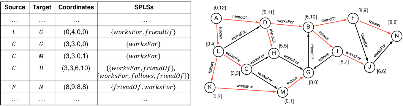
Figure 10. A running example of the index proposed by Jin et al. (Jin et al., 2010).

Query processing. Query processing starts by checking whether the reachability is recorded in the partial GTC. If it is not, then online traversal is performed, where the partial transitive closure is leveraged to answer the reachability query. Online traversal only needs to visit tree edges as the reachability information caused by non-tree edges is already recorded in the partial GTC. In general, a query $Q_{r}(s,t,\alpha)$ is processed by looking for a path from $s$ to $t$ by three steps: online traversal on the spanning tree from $s$ to $u$, partial GTC lookups for the path from $u$ to $v$, and online traversal on the spanning tree from $u$ to $t$. Consider the query $Q_{r}(L,G,(\texttt{worksFor},\texttt{friendOf})^{*})$ in Fig. 10. Since $(\texttt{worksFor},\texttt{friendOf})$ is recorded as an SPLS of $(L,G)$, query result is $True$. For query $Q_{r}(L,G,(\texttt{worksFor},\texttt{follows})^{*})$, using only partial GTC is not sufficient, and the spanning tree needs to be traversed, e.g., performing a DFS from $L$. In general, the query is processed by combining the following reachability information: (1) the DFS from $L$ can visit $C$ in the tree with $\{\texttt{worksFor}\}$; (2) $M$ is reachable from $C$ with $\{\texttt{worksFor}\}$; (3) the DFS from $M$ can visit $G$ in the tree with $\{\texttt{follows}\}$. Finally, True is returned as the query result.

Query optimization. Given the query $Q_{r}(s,t,\alpha)$, the query processing approach outlined above necessitates the execution of online traversals within the spanning tree. These traversals are aimed at identifying a pair of vertices $(u,v)$, where $u$ and $t$ are reachable from $s$ and $v$, respectively, as per $\alpha$, while also confirming the presence of the entry $(u,v)$ within the partial GTC. For example, an instance of $(u,v)$ are $(C,M)$ in query $Q_{r}(L,G,(\texttt{worksFor},\texttt{follows})^{*})$. In order to avoid online traversals, two optimization techniques are proposed (Jin et al., 2010), which are based on the interval labeling and the histograms of path-label sets. Two problems need to be solved: (1) searching $(u,v)$ in the partial GTC such that $u$ and $t$ are reachable from $s$ and $v$, respectively, in the spanning tree; (2) the path-label sets from $s$ to $u$ and the ones from $v$ to $t$ satisfy the constraint. Two optimizations are discussed below to address these problems. Consequently, queries are processed with only index lookups without any traversal.

Query optimization: the interval labeling. This addresses the issue of checking whether there exists $(u,v)$ in the partial GTC such that $u$ and $t$ are reachable from $s$ and $v$ in the spanning tree. The idea is to achieve this by a multi-dimensional search based on interval labeling. Specifically, after computing the interval labeling on the spanning tree, each vertex obtains an interval (see Section 3.1). Then, given $s$ and $t$, the search looks for $(u,v)$ such that the corresponding intervals can satisfy the following constraint: $[u_{a},u_{b}]$ is subsumed by $[s_{a},s_{b}]$, and $[t_{a},t_{b}]$ is subsumed by $[v_{a},v_{b}]$, which represents that $u$ and $t$ are reachable from $s$ and $v$, respectively, on the spanning tree. Therefore, $(u_{a},u_{b},v_{a},v_{b})$ should satisfy the following $4$ ranges: $s_{a}\leq u_{a}\leq s_{b}$; $s_{a}\leq u_{b}\leq s_{b}$; $0\leq v_{a}\leq t_{a}$; $t_{b}\leq v_{b}\leq|V|-1.$ With these four ranges, the search can be reduced to a four-dimensional search problem. A k-d tree (Bentley, 1975) can be built on the coordinates of the partial GTC to accelerate the searching.

Query optimization: histograms of path-label sets. Interval labeling can deal with the plain reachability information from $s$ to $u$ and from $v$ to $t$. However, the path-label sets from $s$ to $u$ and from $v$ to $t$ on the spanning tree need to be checked for the evaluation of the path constraint. To avoid online traversal for computing such path-label sets, a histogram-based optimization can be adopted. The idea is to record for each vertex $x$ in the tree the occurrence of each edge label in the path from the root $r$ of the tree to $x$, e.g., if the sequence of the edge labels in the path from $r$ to $x$ is $(\texttt{friendOf},\texttt{worksFor},\texttt{friendOf})$, the histogram of $x$, referred to as $H(x)$, is $\{\texttt{friendOf}:2,\texttt{worksFor}:1\}$. With the histograms, the path-label set of the path from $s$ to $u$ (or from $v$ to $t$) in the spanning tree can be computed by $H(u)-H(s)$ (or $H(t)-H(v)$).

For the graph in Fig. 10, interval labeling is computed according to the spanning tree highlighted in red. Then, the column Coordinates is added in the partial GTC, which records the coordinates of each entry, e.g., the coordinates of $(F,N)$ are $(8,9,8,8)$ because the intervals of $F$ and $N$ are $[8,9]$ and $[8,8]$, respectively. Consider query $Q_{r}(D,N,(\texttt{worksFor},\texttt{friendOf})^{*})$. According to the intervals of $D$ and $N$, which are $[5,11]$ and $[8,8]$, the intervals of the pair of vertices $(u,v)$ should satisfy: $5\leq u_{a}\leq 11$, $5\leq u_{b}\leq 11$, $0\leq v_{a}\leq 8$, and $8\leq u_{a}\leq 12$. Thus, $(F,N)$ is located as an instance of $(u,v)$ for the search, and the corresponding SPLS can also satisfy the path-constraint. At this step, we find $(F,N)$ such that $F$ is reachable from $D$ in the spanning tree, and $F$ can reach $N$ satisfying the path constraint. The next step is to compute the path-label sets from $D$ to $F$. With the histograms $H(F)=\{\texttt{friendOf}:2,\texttt{worksFor}:1\}$ and $H(D)=\{\texttt{friendOf}:1\}$, we have $H(F)-H(D)=\{\texttt{friendOf}:1,\texttt{worksFor}:1\}$, which means the path-label set from $D$ to $F$ is $\{\texttt{friendOf},\texttt{worksFor}\}$ that can satisfy the path constraint. Thus, the query result is $True$.

The index building algorithm first computes a spanning tree and then computes the partial GTC by iterative computation from each vertex. The impact of the spanning trees on the index size of partial GTC is extensively studied (Jin et al., 2010).

4.1.2. Tree-based indexes: Chen et al. (Chen and Singh, 2021)

Another tree-based index for alternation-based queries deals with the problem of reachability caused by non-tree edges by using graph decomposition. An input graph $G$ is decomposed into $\mathcal{T}$ and $G_{c}$. $\mathcal{T}$ is an extended spanning tree, and interval labeling can be used to process reachability within $\mathcal{T}$. $G_{c}$ is a graph summary, including reachability that cannot be covered by interval labeling. The decomposition is done recursively generating $(\mathcal{T}^{i},G^{i}_{c})$ where $i$ denotes the iteration, and continues until the decomposition result of a graph summary only contains an extended tree. The objective is to maximally leverage interval labeling to compress the transitive closure. Specifically, for each decomposition result $(\mathcal{T}^{i},G^{i}_{c})$, the interval labeling with histograms (see Section 4.1.1) is computed on $\mathcal{T}^{i}$, which is used as the index for $\mathcal{T}^{i}$. The series of the indexes on $(\mathcal{T}^{1},...,\mathcal{T}^{i},...,\mathcal{T}^{n})$ serves as the index. Query $Q_{r}(s,t,\alpha)$ is decomposed into subqueries that are processed using the series of the indexes.

Edge classification and extended trees. The definition of extended trees is based on a classification of edges as either a tree edge on the spanning tree or a non-tree edge. In Fig. 11, tree edges are highlighted in red. Each non-tree edge $(u,v)$ can be further classified. If there is already a path from $u$ to $v$ in the tree, then $(u,v)$ is a forward edge, e.g., $(A,D)$ in orange in Fig. 11. If $u$ and $v$ are not on the same path in the tree, then $(u,v)$ is a cross edge, e.g., $(C,H)$ in blue in Fig. 11. If there is a path from $v$ to $u$ in the tree, then $(u,v)$ is a back edge, e.g., $(I,G)$ in green in Fig. 11. Under the edge classification, an extended tree is a spanning tree with the corresponding forward edges.

Querying processing in extended trees. Interval labeling using histogram is sufficient to record all the reachability information in an extended tree, since each forward edge $(u,v)$ only leads to more path-label sets from $u$ to $v$ as there is already a path in the tree from $u$ to $v$, and such additional path-label sets can be recorded by histograms $H(u)$ and $H(v)$. Since there can be multiple paths from the root to each vertex in the tree, $H(u)$ (or $H(v)$) in this approach are sets of path-label sets augmented with occurrences of edge labels. Consider the extended tree in Fig. 11. For the query $Q_{r}(D,F,(\texttt{worksFor}\cup\texttt{friendOf})^{*})$, the interval of $F$ is subsumed by the interval of $D$, such that $F$ is reachable from $D$ in the extended tree. In addition, we have $H(D)=\{\{\texttt{friendOf}:1\},\{\texttt{follows}:1,\texttt{worksFor}:1\}\}$, and $H(F)=\{\{\texttt{friendOf}:2,\texttt{worksFor}:1\}\}$, such that $H(F)-H(D)=\{\texttt{friendOf}:1,\texttt{worksFor}:1\}\}$, which means that there is a path-label set $\{\texttt{friendOf},\texttt{worksFor}\}$ from $D$ to $F$. Thus, $True$ is returned as query result.

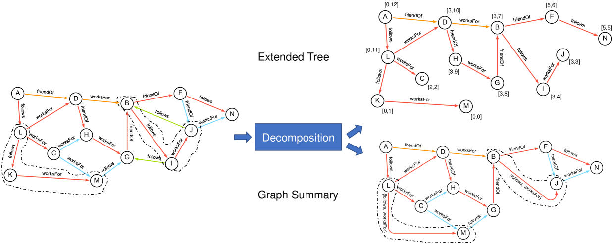
Figure 11. A running example of the index proposed by Chen et al. (Chen and Singh, 2021).

Query decomposition and processing. A query is decomposed into several subqueries, and each of them is evaluated using either an extended tree or a graph summary. As the graph summary can be further decomposed, the subquery on the graph summary will be decomposed correspondingly. Consider Fig. 11 and query $Q_{r}(L,F,\alpha)$ where $\alpha=\{\texttt{worksFor}\cup\texttt{frinedOf}\}^{*}$ is decomposed into $Q_{1}:Q_{r}(L,C,\alpha)$, $Q_{2}:Q_{r}(C,G,\alpha)$, and $Q_{3}:Q_{r}(G,F,\alpha)$. $Q_{1}$ and $Q_{3}$ are processed on the extended tree while $Q_{2}$ on the graph summary. The decomposition is performed by computing two specific sets of vertices for each vertex in the extended tree, denoted as dominant and transferring vertices (see (Chen and Singh, 2021) for formal definitions). $C$ is a dominant vertex for vertex $L$, which means that outgoing reachability with cross edges can be found via $C$. $G$ is a transferring vertex for vertex $F$, which means incoming reachability with cross edges can be found via $G$. The dominant and transferring vertices are computed for vertices in each extended tree.

4.1.3. GTC-based indexes: Zou et al. (Xu et al., 2011; Zou et al., 2014)

The first index in this class is designed based on a transformation from a general graph into an augmented DAG (ADAG) with path-label set information. The transformation also identifies strongly connected components. However, this transformation is more complicated than the one for plain graphs as paths with different sets of labels need to be distinguished. The benefit of performing this transformation is that the generalized transitive closure on the augmented DAG can be computed incrementally in a bottom-up manner. In general, with the transformation, the GTC of the general graph can be computed by combining three kinds of reachability information: reachability inside each SCC, reachability in the ADAG, and reachability between vertices in the ADAG and vertices in the SCCs.

Transformation into the ADAG. The transformation first identifies SCCs in the input graph and then computes two kinds of vertices in each SCC: in-portal vertices and out-portal vertices. In-portal vertices of an SCC have incoming edges from vertices out of the SCC while out-portal vertices of an SCC have outgoing edges to vertices out of the SCC. Then, each SCC is replaced with a bipartite graph with in-portal and out-portal vertices, where edges are labeled with sufficient path-label sets from in-portal to out-portal vertices. Consider the example in Fig. 12, which includes an additional edge $(I,\texttt{worksFor},L)$. The only SCC in the example is highlighted, where in-portal vertices are $\{L,D\}$ and out-portal vertices are $\{B,I\}$. Then, the ADAG is shown in Fig. 12(b) consisting of a bipartite graph with $\{L,D\}$ and $\{B,I\}$. The edge $(L,I)$ in the bipartite graph is labeled $\{\texttt{worksFor,follows}\}$ because it is the only sufficient path-label set from $L$ to $I$ in the SCC.

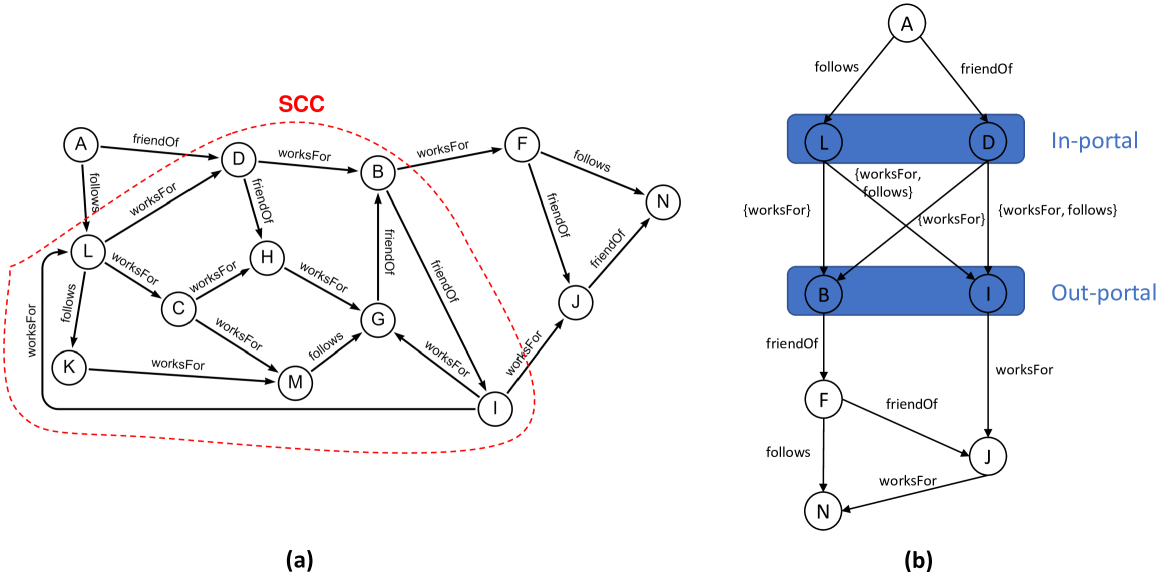
Figure 12. A running example of the index proposed by Zou et al. (Xu et al., 2011; Zou et al., 2014).

Incremental computation of reachability in the ADAG. The reachability in the augmented DAG can be computed in a bottom-up manner according to a topological ordering. Specifically, vertices are examined in the reverse topological order and the single-source GTCs are shared in a bottom-up manner. Note that a single-source GTC is a GTC with a fixed source vertex, i.e., a single-source GTC contains all the vertices that are reachable from a source vertex and the corresponding SPLSs. Consider the example in Fig. 12. In the ADAG, $F$ has an incoming edge from $B$. Then, the single-source GTC of $F$ can be combined with the edge $(B,\texttt{friendOf},F)$ for the computation of the single-source GTC of $B$ in the ADAG.

Computing the reachability within each SCC: a Dijkstra-like algorithm. An interesting algorithm for computing the reachability within each SCC is proposed in the approach. The intuition is to use the number of distinct edge labels in paths to represent the distance between vertices. For instance, in the SCC in Fig. 12(a), there exist two paths from $L$ to $H$: $P1=\{L,\texttt{worksFor},D,\texttt{friendOf},H\}$ and $P2=\{L,\texttt{worksFor},C,\texttt{worksFor},H\}$. In this case, $P2$ is considered as the shorter one as it only has one distinct label. By doing this, Dijkstra’s algorithm can be extended to compute the single-source GTC for vertices in SCCs. In general, ‘shorter’ paths represent paths with sufficient path label sets, which only need to be traversed and recorded in the index.

The reachability from vertices in a SCC to vertices in the ADAG. To compute reachability information, the single-source GTC of in-portal or out-portal vertices can be leveraged. Consider the example in Fig. 12. In order to compute the single-source GTC of $G$ in the entire graph, the sufficient path-label sets from $G$ to the out-portal vertices $B$ and $I$, which are computed by the Dijkstra-like algorithm, are combined with single-source GTCs of $B$ and $I$ that are computed incrementally in the ADAG.

The approach also studies the scalability of the index on large graphs. The intuition is to partition the input graph and compute a local GTC for each partition. Then, a skeleton graph is built over partitions. In general, queries are processed by traversing the skeleton graph with index lookups in each local GTC. In addition, the index can also support dynamic graphs with both edge insertions and deletions.

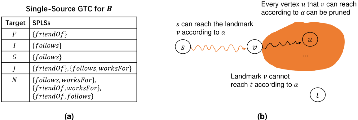
Figure 13. A running of the landmark index proposed by Valstar et al. (Valstar et al., 2017) is presented in (a) for the graph in Fig. 1(b). The pruning technique of the landmark index is illustrated in (b).

4.1.4. GTC-based indexes: Valstar et al. (Valstar et al., 2017)

Landmark index is a partial index, which computes single-source GTCs for a subset of vertices in the graph. The subset of vertices are selected as the top-k vertices in degree ranking, denoted as landmarks. Query $Q_{r}(s,t,\alpha)$ is processed by performing BFS from $s$, which can be accelerated if a landmark vertex is visited by the BFS because the single-source GTC of the landmark records all reachability information from the landmark. Consider the example in Fig. 13, which shows the landmark index for the landmark $B$ in the graph of Fig. 1(b). For processing query $Q_{r}(A,N,\{\texttt{worksFor,follows}\}^{*})$, the BFS from $A$ can visit vertex $B$ according to the path constraint. As $B$ is the landmark, the precomputed single-source GTC of $B$ can be used to evaluate whether $N$ is reachable from $B$ according to the path constraint.

Indexing non-landmark vertices. For each non-landmark vertex, the approach precomputes a fixed number of SPLSs of paths from the non-landmark vertex to each landmark. For instance, in the example in Fig. 13(a), $A$ is a non-landmark vertex, and the approach precomputes $2$ SPLSs from $A$ to $B$, i.e., $\{\texttt{follows,worksFor}\}$ and $\{\texttt{friendOf, worksFor}\}$. With the index entries for $A$, the query processing in the previous example does not require the online BFS from $A$ to $B$ as it can be replaced with index lookups among the index entries of $A$. In case the index entries of a non-landmark vertex cannot satisfy the path constraint in a query, a BFS traversal is still necessary.

Query optimization: pruning techniques for false queries. The major issue in query processing is that the index is not fully leveraged if the query result is actually False. To deal with this issue, a pruning technique is proposed in the approach. Consider Fig. 13 and query $Q_{r}(s,t,\alpha)$. Assume that $s$ can reach the landmark $v$ according to the path constraint specified by $\alpha$. Then, the single-source GTC of $v$ can be used to check whether $t$ is reachable from $v$ according to the path-constraint. In case this is not possible, every vertex $u$ that is reachable from $v$ according to the path constraint can be pruned in the subsequent search of the BFS.

4.1.5. 2-hop-based indexes: Peng et al. (Peng et al., 2020)

P2H+ is a 2-hop index for alternation-based queries, designed based on the transitivity of plain reachability and SPLSs. Given the reachability from $s$ to $u$ and from $u$ to $t$, it is trivial to derive that $t$ is reachable from $s$. In addition, if both paths from $s$ to $u$ and from $u$ to $t$ satisfy the path constraint specified by $\alpha$, the path from $s$ to $t$ can also satisfy the constraint, due to the transitivity of SPLSs (see Section 4.1). Therefore, SPLSs can be added to the index entries of the 2-hop index, which can be used to process alternation-based queries.

The indexing algorithm of P2H+. P2H+ indexing extends the PLL indexing algorithm (Yano et al., 2013) to deal with alternation-based reachability. The P2H+ indexing algorithm intervenes in the second step of the PLL indexing algorithm by computing the SPLSs while performing backward and forward BFS. For example, in Fig. 1, the backward from $B$ can visit $A$ with the path-label set $\{\texttt{worksFor},\texttt{friendOf}\}$. Thus, index entry $(B,(\texttt{worksFor},\texttt{friendOf}))$ is inserted into $L_{out}(A)$.

Pruning rules in the P2H+ indexing. P2H+ applies pruning rules to accelerate index building as well as remove redundancy in the index.

• The first pruning rule is that if vertex $v$ visited by a BFS has been processed previously, then the vertex can be pruned in the subsequent processing steps, since the corresponding reachability information has been recorded when processing $v$.

• The second pruning rule is that an index entry can be skipped if it can be derived from the current snapshot of index. Assume that edge $(D,\texttt{worksFor},F)$ exists in Fig. 1(b). The forward BFS from $D$ can visit $J$ with path-label set $\{\texttt{worksFor},\texttt{friendOf}\}$. If the current snapshot of the index contains $(B,\texttt{worksFor})\in L_{out}(D)$ and $(B,\texttt{friendOf})\in L_{in}(J)$, then the index entry representing the reachability from $D$ to $J$ does not need to be inserted.

• The third pruning rule is to remove redundant index entries while computing SPLSs. In Fig. 1(b), the forward BFS from $L$ can visit $G$ via $M$ with path-label set $\{\texttt{worksFor},\texttt{follows}\}$ and insert $(L,\{\texttt{worksFor},\texttt{follows}\})$ into $L_{in}(G)$. In addition, the BFS can also visit $G$ via $H$ and insert $(L,\{\texttt{worksFor}\})$ into $L_{in}(G)$. The second insertion will make the first insertion redundant because $\{\texttt{worksFor}\}$ is a subset of $\{\texttt{worksFor},\texttt{follows}\}$. To avoid the overhead of insertion followed by deletion, an optimization technique based edge visiting priority is used. The idea is to prioritize the visiting of the edges with labels that have been visited in the BFS. Consequently, the index entries with minimal label sets will be inserted first, which can avoid deleting redundant index entries.

4.1.6. 2-hop-based indexes: Chen et al. (Chen et al., 2022)

DLCR is the latest and the most advanced indexing technique for alternation-based queries. It is an extension of P2H+ to dynamic graphs, in that DLCR is also designed based on the 2-hop index, but allows index updates. DLCR ensures that the index is free of any redundancy following index updates. Consider the toy example in Fig. 14. After inserting edge $(u,v)$ with label $l$ in the graph, $w$ is reachable from $u$ with SPLS $\{l\}$, which needs to be recorded in the index. In addition, $x$ can reach $w$ with $\{l\}$ after the insertion, such that the path from $x$ to $w$ with the label set $\{l,l^{\prime}\}$ becomes redundant, which needs to be deleted from the index. For the case of deleting edge $(u,v)$ with label $l$ in the graph, the reachability information from $x$ to $w$ with $\{l\}$ and from $u$ to $w$ with $\{l\}$ need to be deleted accordingly. In addition, the path from $x$ to $w$ with $\{l,l^{\prime}\}$, which was redundant because of the reachability from $x$ to $w$ with $\{l\}$ before the deletion, needs to be inserted into the index after the edge deletion.

DLCR efficiently updates the index by leveraging the current snapshot of the index to reflect the changes. When inserting an edge $(u,v)$ with label ${l}$, DLCR performs forward BFS from vertex $u$ and backward BFS from vertex $v$ to record additional reachability information. It is important to note that these BFS operations do not start from scratch; instead, they leverage the index entries in $L_{in}(u)$ and $L_{out}(v)$. During the BFS operations, if the corresponding index entries change for any visited vertex, that vertex is marked as an affected vertex, which is used to identify and remove redundant index entries. The process for edge deletion is similar to that of edge insertion. It is worth emphasizing that to completely remove redundancies after edge insertion or to add all necessary index entries after edge deletion, the maintenance of inverted index entries is crucial. For more in-depth information, we direct the readers to the paper (Chen et al., 2022).

We present a running example of index updates in DLCR in Fig. 15, which only includes the information for updating $L_{in}$-entries. For inserting edge $(H,\texttt{worksFor},G)$ in (a), the snapshots of the index are changed from (b) to (d), and (c) is an intermediate snapshot during the updates, which exists after inserting index entries but before deleting any redundancies. For deleting edge $(H,\texttt{worksFor},G)$ in (a), the index is changed from (d) to (b).

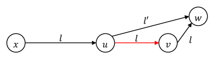
Figure 14. A toy example for illustrating index updates in DLCR proposed by Chen et al. (Chen et al., 2022).

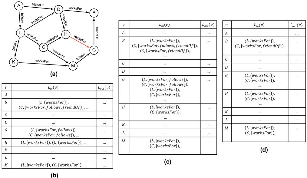
Figure 15. A running example of the index updates in DLCR proposed by Chen et al. (Chen et al., 2022).

4.2. Indexes for concatenation-based queries

In concatenation-based reachability queries, the path constraint defines a label sequence, and the edge labels in the path from the source to the target are repeats of the defined label sequence. In Fig. 1(b), $Q_{r}(L,B,(\texttt{worksFor}\cdot\texttt{friendOf})^{*})=True$ because the sequence of edge labels in the path from $L$ to $B$ via $D$, $H$, and $G$ are repeats of $(\texttt{worksFor},\texttt{friendOf})$. Concatenation-based reachability are supported by SPARQL (Steve and Andy, 2013), SQL/PGQ (Deutsch et al., 2022), GQL (Deutsch et al., 2022).

Minimum repeats. In order to index concatenation-based reachability, path-label sequences from a source to a target are necessary to record (Zhang et al., 2023b), e.g., the path-label sequence of the path from $L$ to $B$ via $D$, $H$, and $G$ in Fig. 1(b) is $(\texttt{worksFor},\texttt{friendOf},\texttt{worksFor},\texttt{friendOf})$. Recording only the minimum repeats, instead of the raw label sequences, is sufficient for concatenation-based reachability query processing (Zhang et al., 2023b), e.g., the minimum repeat of the path from $L$ to $B$ in the previous example is $(\texttt{worksFor},\texttt{friendOf})$.

Kernel-based search. With minimum repeats, the generalized transitive closure that extends the transitive closure with the minimum repeats can be used to process concatenation-based queries. The problem is how to compute the minimum repeats from a source to a target as there can be an infinite number of minimum repeats due to the existence of cycles in the path. Consider the graph in Fig. 1(b) and the problem of computing the minimum repeats from $D$ to $J$. Due to the existence of the cycle including vertices $B$, $I$, and $G$, the potential number of minimum repeats from $D$ to $J$ is infinite (assuming arbitrary path semantics – see Section 2). The solution to the problem is based on a practical observation, that the number of concatenated labels under the Kleene star is usually bounded. Based on the observation, the first reachability index for concatenation-based queries (Zhang et al., 2023b) designs a kernel-based search to compute minimum repeats. The idea is to first compute kernels that are essentially label sequences on the fly and then use the kernels to guide the subsequent search. In the above example with $k\leq 2$, the kernel-based search starts the BFS from $D$, and when the BFS visits $I$ with the label sequence $(\texttt{worksFor},\texttt{friendOf})$, the label sequence is treated as the kernel of this search. Subsequent search will be guided by the kernel and can visit $J$, which means $(\texttt{worksFor},\texttt{friendOf})$ is a minimum repeat from $D$ to $J$. In general, for computing a minimum repeat of length up to $k$ from a source vertex, the kernel-based search will first search all the label sequences $LS$ of length $k$ from the source and take the prefix $LS^{\prime}$ of $LS$ as the kernel such that $LS=(LS^{\prime})^{h}\cdot LS^{\prime\prime}$, where $LS^{\prime\prime}$ is either empty or a prefix of $LS^{\prime}$, and $h\geq 1$.

Transitive minimum repeats. In order to leverage an index class that is more advanced than the transitive closure, minimum repeats need to be transitive, but they are not. For example, in Fig. 1(b), it is not feasible to derive the minimum repeat from $L$ to $I$ for paths via $G$ from the minimum repeat $\{\texttt{worksFor}\}$ from $L$ to $G$ and the minimum repeat $\{\texttt{friendOf}\}$ from $G$ to $I$. The intuition to deal with this problem is to take only equal minimum repeats for the derivation (Zhang et al., 2023b), instead of all the minimum repeats, i.e., given the minimum repeat from $s$ to $v$ is $MR1$ and minimum repeat from $v$ to $t$ is $MR2$, we can derive the minimum repeat from $s$ to $t$ if $MR1=MR2$.

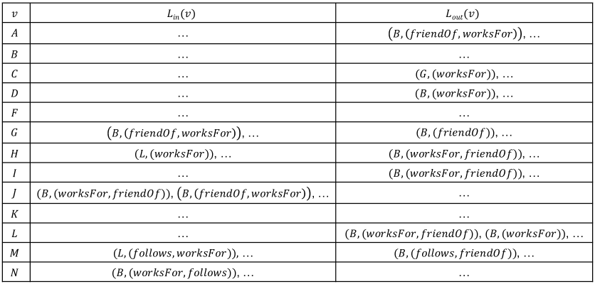
Figure 16. A running example of the RLC index proposed by Zhang et al. (Zhang et al., 2023b) built for the graph in Fig. 1(b).

4.2.1. 2-hop-based indexes: Zhang et al. (Zhang et al., 2023b)

The RLC index is designed based on the 2-hop index for evaluating plain reachability, and the kernel-based search and transitive minimum repeats for computing minimum repeats so as to evaluate concatenation-based path constraint. For instance, in the graph in Fig. 1(a), $B$ is reachable from $L$ with minimum repeat $(\texttt{worksFor},\texttt{friendOf})$, which can be recorded as $(B,(\texttt{worksFor},\texttt{friendOf}))\in L_{out}(L)$. Similarly, $B$ can reach $J$ with the same minimum repeat, which can be recorded as $(B,(\texttt{worksFor},\texttt{friendOf}))\in L_{in}(J)$. The RLC indexing algorithm extends the PLL indexing algorithm by using kernel-based search to compute minimum repeats. Each kernel-based search consists of two phases: kernel search and kernel BFS, which are used to compute kernels and guide the subsequent search using kernels, respectively. The RLC indexing algorithm is equipped with pruning rules to accelerate the index building process, e.g., skipping index entries and vertices during the search. In general, the pruning rules are similar in spirit to the pruning rules in the PLL indexing class for plain reachability, but adapted to the computation of minimum repeats, e.g., pruning rules for skipping vertices can only be applied in the phase of kernel BFS in the RLC indexing algorithm. For processing $Q_{r}(s,t,\alpha)$ with the RLC index, the index entries of $L_{(}out)(s)$ and $L_{in}(t)$ are examined to see whether $(t,MR)\in L_{out}(s)$, $(s,MR)\in L_{in}(t)$, or there exist index entries $(v,MR)$ in both $L_{out}(s)$ and $L_{in}(t)$.

We present a running example of the RLC index in Fig. 16, designed to encompass all minimum repeats involving at most $2$ edge labels. This illustrative example exclusively includes index entries relevant to vertices $B$ and $L$. For $Q_{r}(L,J,(\texttt{worksFor}\cdot\texttt{frinedOf})^{*})$, as there exists $(B,(\texttt{worksFor},\texttt{frinedOf}))$ in both $L_{out}(L)$ and $L_{in}(J)$, such that the query result is $True$.

4.3. Complexity

For the index proposed by Jin et al. (Jin et al., 2010), the index construction time is dominated by a procedure for computing all the vertices that a specific vertex can reach, i.e., the SingleSourcePathLabel algorithm in (Jin et al., 2010), which takes $O(|V||E|\binom{|\mathcal{L}|}{|\mathcal{L}|/2})$ time and is repeated for each vertex. The index size is bounded by $O(|V|^{2}\binom{|\mathcal{L}|}{|\mathcal{L}|/2})$. The query time is $O(log(k)+\sum_{i=1}^{k^{\prime}}|NT(u_{i},v_{i})|)$ (see (Jin et al., 2010) for the specific factors in the bound.) As the approach by Chen et al. (Chen and Singh, 2021) is based on recursive graph decomposition, the complexity included factors related to such decomposition (see (Chen and Singh, 2021) for detail).

The approach by Zou et al. (Xu et al., 2011; Zou et al., 2014) computes and stores the generalized transitive closure of input graph, the index size is $O(|V|^{2}\binom{|\mathcal{L}|}{\mathcal{L}/2})$, and the query time is $O(\binom{|\mathcal{L}|}{\mathcal{L}/2})$, i.e., looking for sufficient path-label sets recorded under $(s,t)$. The landmark approach by Valstar et al. (Valstar et al., 2017) computes the single-source GTC for landmark vertices, which takes $O((|V|(\log|V|+2^{|\mathcal{L}|})+|E|)k2^{|\mathcal{L}|})$ time for $k$ landmarks. Indexing $b$ entries for each of $|V|-k$ non-landmark vertices takes $O((|V|(\log|V|+b)+|E|)(|V|-k)2^{|\mathcal{L}|})$ time. The space for landmark vertices is $O(kn2^{|\mathcal{L}|})$ and the space for non-landmark vertices is $O((n-k)b)$. Query processing can visit $k$ landmarks in the worst case, which takes $O(|E|+k(2^{|\mathcal{L}|}+|V|))$ time.

In the P2H+ approach by Peng et al. (Peng et al., 2020), each BFS for computing index entries takes $O(|E||V|2^{2|\mathcal{L}|})$ time, which is repeated for each vertex. Each $L_{in}(v)$ or $L_{out}(v)$ can take $O(n2^{|\mathcal{L}|})$ space. For the query processing, a merge join is performed between $L_{out}(s)$ and $L_{in}(t)$. As DLCR by Chen et al. (Chen et al., 2022) is essentially equivalent to P2H+ on static graphs, it has the same complexity. The main advantage of DLCR over P2H+ is index updates on dynamic graphs. Edge insertion and deletion take $O(2^{2|\mathcal{L}|}|V|(|\mathcal{L}_{add}||V|+|B|(|V|+|E|)))$ and $O((|B|(|\mathcal{L}|+\log|V|)+|C|2^{2|\mathcal{L}|}|V|)(|V|+|E|))$ time, respectively (see (Chen et al., 2022) for the specific factors).

The RLC index proposed by Zhang et al. (Zhang et al., 2023b) is built by performing kernel search and kernel BFS from each vertex. The kernel search from each vertex takes $O(|\mathcal{L}|^{k}|V|^{k})$ time, which can generate $O(|\mathcal{L}|^{k})$ kernels, and the kernel BFS for each kernel takes $O(|E|k)$ time. Each $L_{out}(v)$ or $L_{in}(v)$ can have $O(|V||\mathcal{L}|^{k})$ entries. Query processing is based on a merge join, which takes $O(|L_{out}(s)|+|L_{in}(t)|)$ time.

5. Open Challenges

Despite the abundance of proposed methods, there are still challenges in incorporating full-fledged indexes in modern graph database management systems (GDBMs). One of the main challenges is that real-world graphs are large and fully dynamic with both edge insertions and deletions. Thus, indexes should be able to scale to large graphs and should be able to accommodate efficient index updates. There are particular challenges for path-constrained reachability indexes due to the variations in query formalization, including path constraints and path semantics. Furthermore, leveraging path-constrained indexes for efficiently processing the entire fragment of regular path queries is also a promising research direction. Finally, parallel indexing to further reduce indexing time has not been well studied. In this section, we elaborate on these challenges and discuss the corresponding research perspectives.

5.1. Large dynamic graphs

Scalability of plain reachability indexes. The state-of-the art plain reachability indexes can be built efficiently on large graphs. For instance, given a graph with 3 million vertices and 16 million edges, BFL (Su et al., 2017) can be built in 1.3 seconds, and the index size is 132 megabytes. Query processing using BFL only requires 0.26 microseconds per query on average. This efficiency is achieved by using partial indexes rather than complete indexes. Complete indexes record the reachability information for any pair of vertices, increasing the indexing cost but reducing query latency as a few index lookups are sufficient. Partial indexes do not record the reachability information for every pair of vertices, reducing the indexing cost, but increasing query latency since graph traversal is needed. We analyzed the existing indexing techniques and found a clear evolution in designing plain reachability indexes. Early plain reachability indexes are complete indexes, e.g., tree cover (Agrawal et al., 1989) and 2-hop (Cohen et al., 2003) indexes, followed by the partial indexes without false positives, e.g., GRIPP (Trißl and Leser, 2007). The latest plain reachability indexes are partial indexes without false negatives, e.g., BFL (Su et al., 2017). Although both types of partial indexes might require traversing the input graph for query evaluation, the design of partial indexes without false negatives is preferable than the one without false positives. The main reason is that the reachability ratio in real-world graphs, which is the number of reachable pairs of vertices divided by the total number of vertices in the graph, is very small (Su et al., 2017). Consequently, the actual result of a given query is likely to be $False$, which means that using a partial index without false negatives can immediately return the query result.

Challenges for plain reachability indexes. The main challenge for plain reachability indexes is that partial indexes without false negatives are mainly designed for static graphs, and a recent work, i.e., DBL (Lyu et al., 2021), can only support insertion-only graphs. Designing partial indexes without false negatives for dynamic or streaming graphs remains an open challenge.

Challenges for path-constrained reachability indexes. The reachability ratio for path-constrained reachability queries can be even lower because the queries will further apply a path constraint to all retrieved paths from source to target. This calls for the design of a partial index without false negatives. However, the only partial index for path-constrained reachability in the literature is landmark index (Valstar et al., 2017), which is a partial index without false positives and can only support static graphs. Although DLCR (Chen et al., 2022) can support dynamic graphs, it is a complete index and the corresponding indexing cost can be high on large graphs. For path-constrained reachability queries, designing partial indexes without false negatives for dynamic or streaming graphs remains an open challenge.

5.2. Various formalisation in path-constrained reachability queries

General path constraints. Existing path-constrained reachability indexes can only support a specific type of path constraints: either alternation-based or concatenation-based. However, path constraints occurring in real-world query logs belong to several classes (Bonifati et al., 2019), e.g., $a^{*}\cdot b^{*}$, $(a_{1}\cup...\cup a_{k})\cdot b^{*}$, etc., where $a$ and $b$ represent edge labels. Designing reachability indexes for queries with more general path constraints is an open research direction.

Different path semantics. Evaluation of path-constrained queries can be based on various path semantics. However, current indexes can only support specific path semantics. Concatenation-based indexes (Zhang et al., 2023b) are designed for arbitrary path semantics, where vertices can be traversed an arbitrary number of times. Alternation-based indexes (Jin et al., 2010; Zou et al., 2014; Valstar et al., 2017; Peng et al., 2020; Chen and Singh, 2021) can be used to evaluate queries based on both simple (non-repeated edges) and arbitrary path semantics as the foundation for building these indexes, i.e., sufficient path label sets, can naturally remove the repeated visiting of edges. In the new standard graph query languages, such as GQL and SQL/PGQ (Deutsch et al., 2022), queries can combine restrictors and selectors, which leads to query processing using different path semantics. Restrictors are path predicates so that the number of matches is not infinite. For instance, ACYCLIC imposes non-repeated nodes including origin and destination. Selectors are the algorithms that compute the partitions of paths. For instance, ALL SHORTEST will partition the solution space into groups of equal-length paths and eventually select the shortest ones. Therefore, choosing any combinations of restrictors and selectors controls the finite sets of matches and also the results. A plethora of indexes can be designed to cover various combinations of selectors and restrictors, out of which those studied in current standard graph query languages.

5.3. Reachability indexes on property graphs

Reachability queries on property graphs include predicates on the edge and vertex properties, referred to as property predicates. Property predicates impose additional constraints on the selection of paths from the source to the target. Existing indexes are not sufficient to process reachability queries on property graphs since they only index graph topology. A theoretical study (Libkin and Vrgoč, 2012) characterizes property predicates that are tractable based on register automata. However, indexing property graphs for reachability has not been studied and remains an important challenge.

5.4. Parallel indexing

Existing indexing algorithms use only a single thread for building the index. To further improve the indexing performance, it is important to parallelize. There are a few recent advances on parallel computation of the 2-hop index (Li et al., 2019; Jin et al., 2020), where the intuition is to leverage the vertex-centric parallel computing paradigm for computing the labels $L_{out}(v)$ and $L_{in}(v)$. Such parallel computing techniques might pave the way to the design of parallel indexing of path-constrained reachability queries as the latest indexes are also designed based on the 2-hop index.

5.5. Incorporating reachability indexes in GDBMSs

Most existing work consider reachability index in isolation rather than as part of a GDBMS. A few existing approaches (Kuijpers et al., 2021; Sumrall et al., 2017; Fletcher et al., 2016) focus on materializing paths of a fixed length and store such paths in a B+ tree. Incorporating reachability indexes into modern GDBMSs remains an open challenge, where the main problem is how to leverage reachability indexes for accelerating the processing of recursive graph queries. An early study (Gubichev et al., 2013) incorporates Ferrari (Seufert et al., 2013) into RDF-3X (Neumann and Weikum, 2008) and demonstrates interesting results for processing queries with Kleene star in SPARQL. Studying the integration of recent indexing techniques for path-constrained queries into GDBMs to support arbitrarily complex recursive graph queries is another relevant research direction to address.

References

- (1)
- Abiteboul and Vianu (1997) Serge Abiteboul and Victor Vianu. 1997. Regular Path Queries with Constraints. In Proc. 16th ACM SIGACT-SIGMOD-SIGART Symp. on Principles of Database Systems. 122–133. https://doi.org/10.1145/263661.263676
- Agrawal et al. (1989) R. Agrawal, A. Borgida, and H. V. Jagadish. 1989. Efficient Management of Transitive Relationships in Large Data and Knowledge Bases. In Proc. ACM SIGMOD Int. Conf. on Management of Data. 253–262. https://doi.org/10.1145/67544.66950
- Angles (2012) Renzo Angles. 2012. A Comparison of Current Graph Database Models. In Proc. Workshops of 28th Int. Conf. on Data Engineering. 171–177. https://doi.org/10.1109/ICDEW.2012.31
- Angles et al. (2017) Renzo Angles, Marcelo Arenas, Pablo Barceló, Aidan Hogan, Juan Reutter, and Domagoj Vrgoč. 2017. Foundations of Modern Query Languages for Graph Databases. ACM Comput. Surv. 50, 5, Article 68 (2017), 40 pages. https://doi.org/10.1145/3104031
- Angles and Gutierrez (2008) Renzo Angles and Claudio Gutierrez. 2008. Survey of Graph Database Models. ACM Comput. Surv. 40, 1, Article 1 (feb 2008), 39 pages. https://doi.org/10.1145/1322432.1322433
- Angles and Gutierrez (2018) Renzo Angles and Claudio Gutierrez. 2018. An Introduction to Graph Data Management. In Graph Data Management, Fundamental Issues and Recent Developments. 1–32. https://doi.org/10.1007/978-3-319-96193-4_1
- Barceló et al. (2012) Pablo Barceló, Leonid Libkin, Anthony W. Lin, and Peter T. Wood. 2012. Expressive Languages for Path Queries over Graph-Structured Data. ACM Trans. Database Syst. 37, 4, Article 31 (2012), 46 pages. https://doi.org/10.1145/2389241.2389250
- Barceló Baeza (2013) Pablo Barceló Baeza. 2013. Querying Graph Databases. In Proc. 32nd ACM SIGACT-SIGMOD-SIGART Symp. on Principles of Database Systems. 175–188. https://doi.org/10.1145/2463664.2465216
- Barthélemy (2011) Marc Barthélemy. 2011. Spatial networks. Phys. Rep. 499, 1 (2011), 1–101. https://doi.org/10.1016/j.physrep.2010.11.002
- Bentley (1975) Jon Louis Bentley. 1975. Multidimensional Binary Search Trees Used for Associative Searching. Commun. ACM 18, 9 (1975), 509–517. https://doi.org/10.1145/361002.361007
- Besta et al. (2023) Maciej Besta, Robert Gerstenberger, Emanuel Peter, Marc Fischer, Michał Podstawski, Claude Barthels, Gustavo Alonso, and Torsten Hoefler. 2023. Demystifying Graph Databases: Analysis and Taxonomy of Data Organization, System Designs, and Graph Queries. ACM Comput. Surv. 56, 2, Article 31 (2023), 40 pages. https://doi.org/10.1145/3604932
- Bonifati and Dumbrava (2019) Angela Bonifati and Stefania Dumbrava. 2019. Graph Queries: From Theory to Practice. ACM SIGMOD Rec. 47, 4 (may 2019), 5–16. https://doi.org/10.1145/3335409.3335411
- Bonifati et al. (2018) Angela Bonifati, George Fletcher, Hannes Voigt, and Nikolay Yakovets. 2018. Querying Graphs. Morgan & Claypool Publishers. https://doi.org/10.2200/S00873ED1V01Y201808DTM051
- Bonifati et al. (2019) Angela Bonifati, Wim Martens, and Thomas Timm. 2019. Navigating the Maze of Wikidata Query Logs. In Proc. 28th Int. World Wide Web Conf. 127–138. https://doi.org/10.1145/3308558.3313472
- Bramandia et al. (2010) Ramadhana Bramandia, Byron Choi, and Wee Keong Ng. 2010. Incremental Maintenance of 2-Hop Labeling of Large Graphs. IEEE Trans. Knowl. and Data Eng. 22, 5 (2010), 682–698. https://doi.org/10.1109/TKDE.2009.117
- Bunke (2000) Horst Bunke. 2000. Graph Matching: Theoretical Foundations, Algorithms, and Applications. In Vision Interface. 82–88.
- Cai and Poon (2010) Jing Cai and Chung Keung Poon. 2010. Path-Hop: Efficiently Indexing Large Graphs for Reachability Queries. In Proc. 19th ACM Int. Conf. on Information and Knowledge Management. 119–128. https://doi.org/10.1145/1871437.1871457
- Calvanese et al. (2002) Diego Calvanese, Giuseppe De Giacomo, Maurizio Lenzerini, and Moshe Y. Vardi. 2002. Rewriting of Regular Expressions and Regular Path Queries. J. Comput. Syst. Sci 64, 3 (2002), 443–465. https://doi.org/10.1006/jcss.2001.1805
- Calvanese et al. (2003) D. Calvanese, G. De Giacomo, M. Lenzerini, and M. Y. Vardi. 2003. Reasoning on Regular Path Queries. ACM SIGMOD Rec. 32, 4 (dec 2003), 83–92. https://doi.org/10.1145/959060.959076
- Chen et al. (2005) Li Chen, Amarnath Gupta, and M. Erdem Kurul. 2005. Stack-Based Algorithms for Pattern Matching on DAGs. In Proc. 31st Int. Conf. on Very Large Data Bases. 493–504. https://dl.acm.org/doi/10.5555/1083592.1083651
- Chen et al. (2022) Xin Chen, You Peng, Sibo Wang, and Jeffrey Xu Yu. 2022. DLCR: Efficient Indexing for Label-Constrained Reachability Queries on Large Dynamic Graphs. Proc. VLDB Endowment 15, 8 (2022), 1645–1657. https://doi.org/10.14778/3529337.3529348
- Chen and Chen (2008) Y. Chen and Y. Chen. 2008. An Efficient Algorithm for Answering Graph Reachability Queries. In Proc. 24th Int. Conf. on Data Engineering. 893–902. https://doi.org/10.1109/ICDE.2008.4497498
- Chen and Singh (2021) Yangjun Chen and Gagandeep Singh. 2021. Graph Indexing for Efficient Evaluation of Label-constrained Reachability Queries. ACM Trans. Database Syst. 46, 2, Article 8 (2021), 50 pages. https://doi.org/10.1145/3451159
- Cheng et al. (2013) James Cheng, Silu Huang, Huanhuan Wu, and Ada Wai-Chee Fu. 2013. TF-Label: A Topological-Folding Labeling Scheme for Reachability Querying in a Large Graph. In Proc. ACM SIGMOD Int. Conf. on Management of Data. 193–204. https://doi.org/10.1145/2463676.2465286
- Cohen et al. (2003) Edith Cohen, Eran Halperin, Haim Kaplan, and Uri Zwick. 2003. Reachability and Distance Queries via 2-Hop Labels. SIAM J. on Comput. 32, 5 (2003), 1338–1355. https://doi.org/10.1137/S0097539702403098
- Deutsch et al. (2022) Alin Deutsch, Nadime Francis, Alastair Green, Keith Hare, Bei Li, Leonid Libkin, Tobias Lindaaker, Victor Marsault, Wim Martens, Jan Michels, Filip Murlak, Stefan Plantikow, Petra Selmer, Oskar van Rest, Hannes Voigt, Domagoj Vrgoč, Mingxi Wu, and Fred Zemke. 2022. Graph Pattern Matching in GQL and SQL/PGQ. In Proc. ACM SIGMOD Int. Conf. on Management of Data. 2246–2258. https://doi.org/10.1145/3514221.3526057
- Erling et al. (2015) Orri Erling, Alex Averbuch, Josep Larriba-Pey, Hassan Chafi, Andrey Gubichev, Arnau Prat, Minh-Duc Pham, and Peter Boncz. 2015. The LDBC Social Network Benchmark: Interactive Workload. In Proc. ACM SIGMOD Int. Conf. on Management of Data. 619–630. https://doi.org/10.1145/2723372.2742786
- Fan et al. (2011) Wenfei Fan, Jianzhong Li, Shuai Ma, Nan Tang, and Yinghui Wu. 2011. Adding regular expressions to graph reachability and pattern queries. In Proc. 27th Int. Conf. on Data Engineering. 39–50. https://doi.org/10.1109/ICDE.2011.5767858
- Fletcher and Theobald (2018) George Fletcher and Martin Theobald. 2018. Indexing for Graph Query Evaluation. In Encyclopedia of Big Data Technologies. 1–9. https://doi.org/10.1007/978-3-319-63962-8_212-1
- Fletcher et al. (2016) George HL Fletcher, Jeroen Peters, and Alexandra Poulovassilis. 2016. Efficient regular path query evaluation using path indexes. In Proc. 19th Int. Conf. on Extending Database Technology. 636–639.
- Foulds (1992) L. R. Foulds. 1992. Digraphs. In Graph Theory Applications. 93–122. https://doi.org/10.1007/978-1-4612-0933-1_7
- Gallagher (2006) Brian Gallagher. 2006. Matching Structure and Semantics: A Survey on Graph-Based Pattern Matching.. In Proceedings of the AAAI Fall Symposium. 43–53.
- Gubichev et al. (2013) Andrey Gubichev, Srikanta J. Bedathur, and Stephan Seufert. 2013. Sparqling Kleene: Fast Property Paths in RDF-3X. In Proc. 1st Int. Workshop on Graph Data Management Experiences & Systems. 7 pages. https://doi.org/10.1145/2484425.2484443
- Gutierrez and Sequeda (2021) Claudio Gutierrez and Juan F. Sequeda. 2021. Knowledge Graphs. Commun. ACM 64, 3 (2021), 96–104. https://doi.org/10.1145/3418294
- Haixun Wang et al. (2006) Haixun Wang, Hao He, Jun Yang, P. S. Yu, and J. X. Yu. 2006. Dual Labeling: Answering Graph Reachability Queries in Constant Time. In Proc. 22nd Int. Conf. on Data Engineering. 75–75. https://doi.org/10.1109/ICDE.2006.53
- Hanauer et al. (2020) Kathrin Hanauer, Monika Henzinger, and Christian Schulz. 2020. Fully Dynamic Single-Source Reachability in Practice: An Experimental Study. In Proc. 22nd Symp. on Algorithm Eng. and Experiments. 106–119. https://doi.org/10.1137/1.9781611976007.9
- Hanauer et al. (2022) Kathrin Hanauer, Christian Schulz, and Jonathan Trummer. 2022. O’Reach: Even Faster Reachability in Large Graphs. ACM J. Exp. Algorithmics 27, Article 4.2 (2022), 27 pages. https://doi.org/10.1145/3556540
- Henzinger and King (1995) M.R. Henzinger and V. King. 1995. Fully dynamic biconnectivity and transitive closure. In Proc. 36th Annual Symp. on Foundations of Computer Science. 664–672. https://doi.org/10.1109/SFCS.1995.492668
- Jagadish (1990) H. V. Jagadish. 1990. A Compression Technique to Materialize Transitive Closure. ACM Trans. Database Syst. 15, 4 (1990), 558–598. https://doi.org/10.1145/99935.99944
- Jin et al. (2010) Ruoming Jin, Hui Hong, Haixun Wang, Ning Ruan, and Yang Xiang. 2010. Computing Label-Constraint Reachability in Graph Databases. In Proc. ACM SIGMOD Int. Conf. on Management of Data. 123–134. https://doi.org/10.1145/1807167.1807183
- Jin et al. (2020) Ruoming Jin, Zhen Peng, Wendell Wu, Feodor Dragan, Gagan Agrawal, and Bin Ren. 2020. Parallelizing Pruned Landmark Labeling: Dealing with Dependencies in Graph Algorithms. In Proc. 34th Annual Int. Conf. on Supercomputing. Article 11, 13 pages. https://doi.org/10.1145/3392717.3392745
- Jin et al. (2012) Ruoming Jin, Ning Ruan, Saikat Dey, and Jeffrey Yu Xu. 2012. SCARAB: Scaling Reachability Computation on Large Graphs. In Proc. ACM SIGMOD Int. Conf. on Management of Data. 169–180. https://doi.org/10.1145/2213836.2213856
- Jin et al. (2011) Ruoming Jin, Ning Ruan, Yang Xiang, and Haixun Wang. 2011. Path-Tree: An Efficient Reachability Indexing Scheme for Large Directed Graphs. ACM Trans. Database Syst. 36, 1, Article 7 (2011), 44 pages. https://doi.org/10.1145/1929934.1929941
- Jin and Wang (2013) Ruoming Jin and Guan Wang. 2013. Simple, Fast, and Scalable Reachability Oracle. Proc. VLDB Endowment 6, 14 (2013), 1978–1989. https://doi.org/10.14778/2556549.2556578
- Jin et al. (2009) Ruoming Jin, Yang Xiang, Ning Ruan, and David Fuhry. 2009. 3-HOP: A High-Compression Indexing Scheme for Reachability Query. In Proc. ACM SIGMOD Int. Conf. on Management of Data. 813–826. https://doi.org/10.1145/1559845.1559930
- Jin et al. (2008) Ruoming Jin, Yang Xiang, Ning Ruan, and Haixun Wang. 2008. Efficiently Answering Reachability Queries on Very Large Directed Graphs. In Proc. ACM SIGMOD Int. Conf. on Management of Data. 595–608. https://doi.org/10.1145/1376616.1376677
- Koutrouli et al. (2020) Mikaela Koutrouli, Evangelos Karatzas, David Paez-Espino, and Georgios A Pavlopoulos. 2020. A Guide to Conquer the Biological Network Era Using Graph Theory. Front. Bioeng. Biotechnol. 8 (2020), 34. https://doi.org/10.3389/fbioe.2020.00034
- Kuijpers et al. (2021) Jochem Kuijpers, George Fletcher, Tobias Lindaaker, and Nikolay Yakovets. 2021. Path Indexing in the Cypher Query Pipeline. In Proc. 24th Int. Conf. on Extending Database Technology. 582–587. https://openproceedings.org/2021/conf/edbt/p156.pdf
- Li et al. (2019) Wentao Li, Miao Qiao, Lu Qin, Ying Zhang, Lijun Chang, and Xuemin Lin. 2019. Scaling Distance Labeling on Small-World Networks. In Proc. ACM SIGMOD Int. Conf. on Management of Data. 1060–1077. https://doi.org/10.1145/3299869.3319877
- Libkin and Vrgoč (2012) Leonid Libkin and Domagoj Vrgoč. 2012. Regular Path Queries on Graphs with Data. In Proc. 15th Int. Conf. on Database Theory (Berlin, Germany). 74–85. https://doi.org/10.1145/2274576.2274585
- Livi and Rizzi (2013) Lorenzo Livi and Antonello Rizzi. 2013. The Graph Matching Problem. Pattern Anal. Appl. 16, 3 (aug 2013), 253–283. https://doi.org/10.1007/s10044-012-0284-8
- Lyu et al. (2021) Qiuyi Lyu, Yuchen Li, Bingsheng He, and Bin Gong. 2021. DBL: Efficient Reachability Queries on Dynamic Graphs. In Proc. 26th Int. Conf. on Database Systems for Advanced Applications. 761–777. https://doi.org/10.1007/978-3-030-73197-7_52
- Mathur (2021) Nav Mathur. 2021. White Paper: Neo4j for Financial Services. https://neo4j.com/whitepapers/financial-services-neo4j.
- Merz and Sanders (2014) Florian Merz and Peter Sanders. 2014. PReaCH: A fast lightweight reachability index using pruning and contraction hierarchies. In In Proc. 22th European Symp. on Algorithms. 701–712. https://doi.org/10.1007/978-3-662-44777-2_58
- Neumann and Weikum (2008) Thomas Neumann and Gerhard Weikum. 2008. RDF-3X: A RISC-Style Engine for RDF. Proc. VLDB Endowment 1, 1 (2008), 647–659. https://doi.org/10.14778/1453856.1453927
- Newman (2010) Mark Newman. 2010. Networks: An Introduction. Oxford University Press. https://doi.org/10.1093/acprof:oso/9780199206650.001.0001
- Peng et al. (2020) You Peng, Ying Zhang, Xuemin Lin, Lu Qin, and Wenjie Zhang. 2020. Answering Billion-Scale Label-Constrained Reachability Queries within Microsecond. Proc. VLDB Endowment 13, 6 (2020), 812–825. https://doi.org/10.14778/3380750.3380753
- Riesen et al. (2010) Kaspar Riesen, Xiaoyi Jiang, and Horst Bunke. 2010. Exact and Inexact Graph Matching: Methodology and Applications. In Managing and Mining Graph Data. Vol. 40. 217–247. https://doi.org/10.1007/978-1-4419-6045-0_7
- Roditty (2013) Liam Roditty. 2013. Decremental Maintenance of Strongly Connected Components. In Proc. 24th Annual ACM-SIAM Symp. on Discrete Algorithms. 1143–1150. https://doi.org/10.1137/1.9781611973105.82
- Roditty and Zwick (2004) Liam Roditty and Uri Zwick. 2004. A Fully Dynamic Reachability Algorithm for Directed Graphs with an Almost Linear Update Time. In Proc. 36th Annual ACM Symp. on Theory of Computing. 184–191. https://doi.org/10.1145/1007352.1007387
- Sahu et al. (2017) Siddhartha Sahu, Amine Mhedhbi, Semih Salihoglu, Jimmy Lin, and M. Tamer Özsu. 2017. The Ubiquity of Large Graphs and Surprising Challenges of Graph Processing. Proc. VLDB Endowment 11, 4 (2017), 420–431. https://doi.org/10.1145/3186728.3164139
- Sahu et al. (2020) Siddhartha Sahu, Amine Mhedhbi, Semih Salihoglu, Jimmy Lin, and M Tamer Özsu. 2020. The ubiquity of large graphs and surprising challenges of graph processing: extended survey. VLDB J. 29, 2 (2020), 595–618. https://doi.org/10.1007/s00778-019-00548-x
- Sakr et al. (2021) Sherif Sakr, Angela Bonifati, Hannes Voigt, Alexandru Iosup, Khaled Ammar, Renzo Angles, Walid G. Aref, Marcelo Arenas, Maciej Besta, Peter A. Boncz, Khuzaima Daudjee, Emanuele Della Valle, Stefania Dumbrava, Olaf Hartig, Bernhard Haslhofer, Tim Hegeman, Jan Hidders, Katja Hose, Adriana Iamnitchi, Vasiliki Kalavri, Hugo Kapp, Wim Martens, M. Tamer Özsu, Eric Peukert, Stefan Plantikow, Mohamed Ragab, Matei Ripeanu, Semih Salihoglu, Christian Schulz, Petra Selmer, Juan F. Sequeda, Joshua Shinavier, Gábor Szárnyas, Riccardo Tommasini, Antonino Tumeo, Alexandru Uta, Ana Lucia Varbanescu, Hsiang-Yun Wu, Nikolay Yakovets, Da Yan, and Eiko Yoneki. 2021. The future is big graphs: A community view on graph processing systems. Commun. ACM 64, 9 (2021), 62–71. https://doi.org/10.1145/3434642
- Schenkel et al. (2005) R. Schenkel, A. Theobald, and G. Weikum. 2005. Efficient creation and incremental maintenance of the HOPI index for complex XML document collections. In Proc. 21st Int. Conf. on Data Engineering. 360–371. https://doi.org/10.1109/ICDE.2005.57
- Sengupta et al. (2019) Neha Sengupta, Amitabha Bagchi, Maya Ramanath, and Srikanta Bedathur. 2019. ARROW: Approximating Reachability Using Random Walks Over Web-Scale Graphs. In Proc. 35th Int. Conf. on Data Engineering. 470–481. https://doi.org/10.1109/ICDE.2019.00049
- Seufert et al. (2013) S. Seufert, A. Anand, S. Bedathur, and G. Weikum. 2013. FERRARI: Flexible and efficient reachability range assignment for graph indexing. In Proc. 29th Int. Conf. on Data Engineering. 1009–1020. https://doi.org/10.1109/ICDE.2013.6544893
- Steve and Andy (2013) Harris Steve and Seaborne Andy. 2013. SPARQL 1.1 Query Language. https://www.w3.org/TR/2013/REC-sparql11-overview-20130321/.
- Su et al. (2017) J. Su, Q. Zhu, H. Wei, and J. X. Yu. 2017. Reachability Querying: Can It Be Even Faster? IEEE Trans. Knowl. and Data Eng. 29, 3 (2017), 683–697. https://doi.org/10.1109/TKDE.2016.2631160
- Sumrall et al. (2017) Jonathan M. Sumrall, George H. L. Fletcher, Alexandra Poulovassilis, Johan Svensson, Magnus Vejlstrup, Chris Vest, and Jim Webber. 2017. Investigations on Path Indexing for Graph Databases. In Euro-Par 2016: Parallel Processing Workshops. 532–544.
- Tarjan (1972) Robert Tarjan. 1972. Depth-first search and linear graph algorithms. SIAM J. on Comput. 1, 2 (1972), 146–160. https://doi.org/10.1137/0201010
- Team (2016) The Neo4j Team. 2016. openCypher. http://www.opencypher.org.
- ten Wolde et al. ([n. d.]) Daniel ten Wolde, Tavneet Singh, Gábor Szárnyas, and Peter A. Boncz. [n. d.]. DuckPGQ: Efficient Property Graph Queries in an analytical RDBMS. In Proc. 13th Biennial Conf. on Innovative Data Systems Research. https://www.cidrdb.org/cidr2023/papers/p66-wolde.pdf
- Trißl and Leser (2007) Silke Trißl and Ulf Leser. 2007. Fast and Practical Indexing and Querying of Very Large Graphs. In Proc. ACM SIGMOD Int. Conf. on Management of Data. 845–856. https://doi.org/10.1145/1247480.1247573
- Valstar et al. (2017) Lucien D.J. Valstar, George H.L. Fletcher, and Yuichi Yoshida. 2017. Landmark Indexing for Evaluation of Label-Constrained Reachability Queries. In Proc. ACM SIGMOD Int. Conf. on Management of Data. 345–358. https://doi.org/10.1145/3035918.3035955
- Veloso et al. (2014) Renê Rodrigues Veloso, Loïc Cerf, Wagner Meira Jr., and Mohammed J. Zaki. 2014. Reachability Queries in Very Large Graphs: A Fast Refined Online Search Approach. In Proc. 17th Int. Conf. on Extending Database Technology. 511–522. https://openproceedings.org/EDBT/2014/paper_166.pdf
- Wei et al. (2014) Hao Wei, Jeffrey Xu Yu, Can Lu, and Ruoming Jin. 2014. Reachability Querying: An Independent Permutation Labeling Approach. Proc. VLDB Endowment 7, 12 (2014), 1191–1202. https://doi.org/10.14778/2732977.2732992
- Wei et al. (2018) Hao Wei, Jeffrey Xu Yu, Can Lu, and Ruoming Jin. 2018. Reachability Querying: An Independent Permutation Labeling Approach. VLDB J. 27, 1 (2018), 1–26. https://doi.org/10.1007/s00778-017-0468-3
- Weller (2014) Mathias Weller. 2014. Optimal Hub Labeling is NP-complete. arXiv:1407.8373 [cs.CC]
- Wood (2012) Peter T. Wood. 2012. Query Languages for Graph Databases. ACM SIGMOD Rec. 41, 1 (2012), 50–60. https://doi.org/10.1145/2206869.2206879
- Xu et al. (2011) Kun Xu, Lei Zou, Jeffery Xu Yu, Lei Chen, Yanghua Xiao, and Dongyan Zhao. 2011. Answering Label-Constraint Reachability in Large Graphs. In Proc. 20th ACM Int. Conf. on Information and Knowledge Management. 1595–1600. https://doi.org/10.1145/2063576.2063807
- Yan et al. (2016) Junchi Yan, Xu-Cheng Yin, Weiyao Lin, Cheng Deng, Hongyuan Zha, and Xiaokang Yang. 2016. A Short Survey of Recent Advances in Graph Matching. In Proc. of the 2016 ACM on Int. Conf. on Multimed. Retr. 167–174. https://doi.org/10.1145/2911996.2912035
- Yang et al. (2019) Bohua Yang, Dong Wen, Lu Qin, Ying Zhang, Xubo Wang, and Xuemin Lin. 2019. Fully Dynamic Depth-First Search in Directed Graphs. Proc. VLDB Endowment 13, 2 (oct 2019), 142–154. https://doi.org/10.14778/3364324.3364329
- Yano et al. (2013) Yosuke Yano, Takuya Akiba, Yoichi Iwata, and Yuichi Yoshida. 2013. Fast and Scalable Reachability Queries on Graphs by Pruned Labeling with Landmarks and Paths. In Proc. 22nd ACM Int. Conf. on Information and Knowledge Management. 1601–1606. https://doi.org/10.1145/2505515.2505724
- Yildirim et al. (2010) Hilmi Yildirim, Vineet Chaoji, and Mohammed J. Zaki. 2010. GRAIL: Scalable Reachability Index for Large Graphs. Proc. VLDB Endowment 3, 1–2 (2010), 276–284. https://doi.org/10.14778/1920841.1920879
- Yildirim et al. (2013) Hilmi Yildirim, Vineet Chaoji, and Mohammed J. Zaki. 2013. DAGGER: A Scalable Index for Reachability Queries in Large Dynamic Graphs. arXiv:1301.0977
- Yu and Cheng (2010) Jeffrey Xu Yu and Jiefeng Cheng. 2010. Graph Reachability Queries: A Survey. In Managing and Mining Graph Data. Vol. 40. 181–215. https://doi.org/10.1007/978-1-4419-6045-0_6
- Yue et al. (2023) Pang Yue, Zou Lei, and Liu Yu. 2023. IFCA: Index-Free Community-Aware Reachability Processing Over Large Dynamic Graphs. In Proc. 39th Int. Conf. on Data Engineering. 2211–2225. https://doi.org/10.1109/ICDE55515.2023.00172
- Zhang et al. (2023b) Chao Zhang, Angela Bonifati, Hugo Kapp, Vlad Ioan Haprian, and Jean-Pierre Lozi. 2023b. A Reachability Index for Recursive Label-Concatenated Graph Queries. In Proc. 39th Int. Conf. on Data Engineering. 66–80. https://doi.org/10.1109/ICDE55515.2023.00013
- Zhang et al. (2023a) Chao Zhang, Angela Bonifati, and M. Tamer Özsu. 2023a. An Overview of Reachability Indexes on Graphs. In Companion of ACM SIGMOD Int. Conf. on Management of Data. 61–68. https://doi.org/10.1145/3555041.3589408
- Zhou et al. (2023) Junfeng Zhou, Jeffrey Xu Yu, Yaxian Qiu, Xian Tang, Ziyang Chen, and Ming Du. 2023. Fast Reachability Queries Answering Based on RCN Reduction. IEEE Trans. Knowl. and Data Eng. 35, 3 (2023), 2590–2609. https://doi.org/10.1109/TKDE.2021.3108433
- Zhou et al. (2017) Junfeng Zhou, Shijie Zhou, Jeffrey Xu Yu, Hao Wei, Ziyang Chen, and Xian Tang. 2017. DAG Reduction: Fast Answering Reachability Queries. In Proc. ACM SIGMOD Int. Conf. on Management of Data. 375–390. https://doi.org/10.1145/3035918.3035927
- Zhu et al. (2014) Andy Diwen Zhu, Wenqing Lin, Sibo Wang, and Xiaokui Xiao. 2014. Reachability Queries on Large Dynamic Graphs: A Total Order Approach. In Proc. ACM SIGMOD Int. Conf. on Management of Data. 1323–1334. https://doi.org/10.1145/2588555.2612181
- Zou et al. (2014) Lei Zou, Kun Xu, Jeffrey Xu Yu, Lei Chen, Yanghua Xiao, and Dongyan Zhao. 2014. Efficient Processing of Label-Constraint Reachability Queries in Large Graphs. Inf. Syst. 40 (March 2014), 47–66. https://doi.org/10.1016/j.is.2013.10.003
- Özsu (2016) M. Tamer Özsu. 2016. A survey of RDF data management systems. Frontiers of Computer Science 10 (April 2016), 418–432. https://doi.org/10.1007/s11704-016-5554-y