On an Optimal Stopping Problem
with a Discontinuous Reward

Abstract.

We study an optimal stopping problem with an unbounded, time-dependent and discontinuous reward function. This problem is motivated by the pricing of a variable annuity contract with guaranteed minimum maturity benefit, under the assumption that the policyholder’s surrender behaviour maximizes the risk-neutral value of the contract. We consider a general fee and surrender charge function, and give a condition under which optimal stopping always occurs at maturity. Using an alternative representation for the value function of the optimization problem, we study its analytical properties and the resulting surrender (or exercise) region. In particular, we show that the non-emptiness and the shape of the surrender region are fully characterized by the fee and the surrender charge functions, which provides a powerful tool to understand their interrelation and how it affects early surrenders and the optimal surrender boundary. Under certain conditions on these two functions, we develop three representations for the value function; two are analogous to their American option counterpart, and one is new to the actuarial and American option pricing literature.    
Keywords: Variable annuities, surrender option, optimal stopping, American options, optimal surrender boundary, early exercise premium, free-boundary value problem, variational inequalities, continuous-time Markov chain approximation.

JEL Classifications: C63, G12, G13, G22

1. Introduction

Variable annuities (VA) are structured products sold by insurance companies that are mainly used for retirement planning. An initial premium is deposited in an investment account (or fund) whose return is linked that of one or more risky assets. They are similar to mutual funds, but they also offer financial guarantees at the end of a pre-determined accumulation period. The embedded guarantees are akin to long-dated options, but they are funded by a periodic fee, generally set as a percentage of the investment account value, rather than being paid upfront. In this paper, we focus on a guaranteed minimum maturity benefit (GMMB), which provides the policyholder a minimum guaranteed amount at maturity of the contract. Another common feature of variable annuities contracts is that policyholders generally have the right to surrender, or lapse, their contract prior to maturity. When policyholders choose to do so, they receive the value accumulated in the investment account, reduced by a penalty for early surrender (or surrender charge). The uncertainty faced by VA providers with respect to early termination is known as surrender risk. Early surrenders can entail negative consequences such as liquidity issues. Thus, incorporating adequate surrender assumptions in the pricing of VAs is essential for risk management purposes; see Niittuinperä (2022).

Different early surrender modelling approaches have been proposed in the literature (see Bauer et al. (2017) and Feng et al. (2022) for a review), from the use of utility functions, Gao and Ulm (2012), to modern statistical techniques, Zhu and Welsch (2015). Early surrenders are also often expressed as a decision taken by policyholders on a strictly rational basis, meaning that the contract is terminated as soon as it is optimal to do so from a financial perspective (see Bernard et al. (2014a), Jeon and Kwak (2018), Kang and Ziveyi (2018), MacKay et al. (2023), and Milevsky and Salisbury (2001), among others). Bauer et al. (2017) discusses the impact of other factors on policyholder behavior, such as taxes and expenses. This article gave rise to another stream of literature in which market frictions such as taxation rules are considered (Alonso-García et al. (2022), Bauer and Moenig (2023), and Moenig and Bauer (2016)), which helps to explain the discrepancies between market and model fee rates, Moenig and Bauer (2016). Other recent studies include lapse and reentry strategies in their analysis (Bernard and Moenig (2019) and Moenig and Zhu (2018)), whereas Moenig and Zhu (2021) consider a third-party investor to whom the policyholder can sell her contract.

The goal of this paper is to study the properties of the value function of the VA contract under the assumption that the policyholder maximizes its risk-neutral value, when the fee and the surrender penalty (or charge) are both time and state-dependent (that is, depending on the value of the VA account, see Bernard et al. (2014a)). Our setup includes, among others, the constant fee case, the state-dependent fees of Bernard et al. (2014a), Delong (2014), and MacKay et al. (2017), and the time-dependent fees of Bernard and Moenig (2019) and Kirkby and Aguilar (2023). Under this assumption, valuing a variable annuity contract is equivalent to solving an optimal stopping problem similar to pricing an American option. However, the financial guarantee being applied only at maturity in a VA contract creates a discontinuity in the reward function at maturity, which sets it apart from the continuous reward function of the American option and complicates the optimal stopping problem involved in the pricing of VAs. The impact of the surrender charge and the fee structure on the optimal surrender strategy has been studied in the Black-Scholes framework by Bernard et al. (2014a), Bernard and MacKay (2015), Bernard and Moenig (2019), MacKay (2014), MacKay et al. (2017), and Moenig and Zhu (2018), and in a more general setting by Kang and Ziveyi (2018) and MacKay et al. (2023). However, these articles approach the problem from a numerical perspective. To the author’s knowledge, it is the first time that such an extensive analytical study of the optimal stopping problem involved in the pricing of a variable annuity contract is performed in the literature.

Recently, Luo and Xing (2021) studied variable annuity contracts under regime-switching volatility models from an optimal stopping perspective. However, they consider a different surrender benefit, which results a continuous reward function similar to that of a put option. Chiarolla et al. (2022) perform an analysis similar to ours, but for participating policies with minimum rate guarantee and surrender option. Participating policies are akin to variable annuities in that the premium paid by the policyholder tracks a financial portfolio, subject to a minimum rate guarantee. However, the problem they consider is fundamentally different from ours in multiple ways. i) In variable annuity contracts, guarantees are funded via periodic fees set as a percentage of the sub-account value. This creates a discrepancy between the fee amount and the value of the financial guarantee, which becomes an incentive for the policyholder to surrender the policy early (Milevsky and Salisbury (2001)). In participating policies, there is no such ongoing fee; upon termination or at maturity, the policyholder receives the reserve and a given percentage of the surplus, defined as a percentage of the tracking portfolio over the policy reserve (the intrinsic value). ii) In variable annuities, the surrender value differs from that of the maturity payout, which creates a time discontinuity in the reward function at maturity; whereas in participating policies, the intrinsic value is paid at maturity or upon early termination, so that the reward function is independent of time and continuous. iii) In participating policies, the contract is terminated if the underlying portfolio falls below the reserve. There is no such feature in a variable annuity, that is, early termination is at the sole discretion of the policyholder. The resulting optimal stopping problem we study in this paper is thus very different from the one considered by Chiarolla et al. (2022), even if they are motivated by similar insurance products.

The time discontinuity and the unboundedness of the reward function involved in the pricing of variable annuities with GMMB prevent the simple application of results from the American option pricing literature to our problem. For example, to express the value function as the solution to a free-boundary value problem, one needs to establish its continuity. However, continuity of the value function often follows from the continuity of the reward function, which, in our setting, is unbounded and only upper semi-continuous, making the results usually cited in the context of American options inapplicable (see, for instance, Bassan and Ceci (2002), Bensoussan and Lions (1982), De Angelis and Stabile (2019), Jaillet et al. (1990), Krylov (1980), and Lamberton (2009)). In this paper, following the work of Van Moerbeke (1974) and Palczewski and Stettner (2010) (in the context of impulse control problems), we establish continuity of the value function by showing that it admits an alternative representation in terms of a continuous reward function. We can then confirm that it is a solution to a free-boundary value problem and prove further properties, which provides enough regularity to apply a generalized version of Itô’s formula to the value process. This allows us to derive various integral representations for the value function, thus extending the results of Bernard et al. (2014b) to general time-dependent fee and surrender charge functions and introducing a new decomposition, the continuation premium representation, to the literature on VA pricing.

The shape and the (non-)emptiness of the exercise region of an American option with a time-homogeneous reward function has first been studied rigorously by Villeneuve (1999). Other authors, such as Jönsson et al. (2006), Kotlow (1973), and Villeneuve (2007), also studied the conditions under which the exercise region has a particular shape. These results are however not directly applicable to the problem we study in this paper, because of the time-dependence and the discontinuity of our reward function. Under the assumption of a general fee and surrender charge structure, we are nonetheless able to identify a condition, expressed as a partial differential inequality, under which the optimal stopping time is always at maturity of the contract, thus mitigating surrender risk. This condition provides a powerful tool to understand the interplay between the fees and surrender charges, and its effect on the optimal stopping strategy. It can also be used to further study and characterize the shape of the optimal exercise, or surrender, region. In particular, we show that the surrender region can be a disconnected set and that the optimal surrender boundary can be discontinuous, thus illustrating a major difference between the pricing of VA contracts and standard American options. Our results extend the work of Milevsky and Salisbury (2001), who consider an infinite horizon, to a more general finite horizon problem.

Our results on the shape of the surrender region also shed light on the link between our original optimal stopping problem and its continuous reward function counterpart. In particular, we obtain conditions under which the two reward functions lead to equivalent optimal stopping problems; that is, we identify cases when they present the same surrender regions and optimal stopping times. While the idea of using an alternate continuous reward process to obtain continuity of the value function is not new to the literature, it is the first time, to the authors’ knowledge, that an in-depth comparison of the two problems is presented.

The main contributions of this paper are listed below.

• We give a condition under which it is never optimal for the policyholder to surrender before maturity of the VA contract.

• We present an alternative representation for the value function of the VA contract in terms of a continuous reward function. This representation is used to perform a rigorous theoretical study of the value function. Our results justify the use of various numerical methods already applied to VA pricing in the literature.

• We provide two integral representations for the value function, which are used to further analyze the value of a VA contract and to characterize the (non-) emptiness of the surrender region. The continuation premium decomposition is new to the actuarial and American option pricing literature and allows for the development of new valuation methods for variable annuity contracts.

• We obtain conditions under which the original optimal stopping problem and the one with an alternative continuous reward function are equivalent.

This paper is organized as follows. Section 2 presents the optimal stopping problem involved in the pricing of VA contracts with a GMMB. The existence of an optimal stopping time is discussed in Section 3. In Section 4, we obtain analytical properties of the value function, derive its integral representations and study the shape of the surrender region. We also discuss the equivalence between the original optimal stopping problem and its continuous reward function counterpart. Numerical examples are provided in Section 5. Section 6 concludes the paper.

2. Financial Setting

2.1. Market Model

On a probability space $(\Omega,\mathcal{F},\mathbb{Q})$, let $W=\{W_{t}\}_{t\geq 0}$ be a standard Brownian motion whose augmented filtration is denoted by $\mathbb{F}=\{\mathcal{F}_{t}\}_{t\geq 0}$. $\mathbb{Q}$ is the probability measure used to price assets presented below.

We consider a financial market consisting of two primary assets, a risk-free bond $B=\{B_{t}\}_{t\geq 0}$ and a risky asset $S=\{S_{t}\}_{t\geq 0}$ whose dynamics under the measure $\mathbb{Q}$ are given by

(1) $$\begin{array}[]{rll}\,\mathrm{d}B_{t}&=&rB_{t}\,\mathrm{d}t,\\ \,\mathrm{d}S_{t}&=&rS_{t}\,\mathrm{d}t+\sigma S_{t}\,\mathrm{d}W_{t},\end{array}$$

where $r$, $\sigma$ are deterministic constants with $\sigma>0$, and $W=\{W_{t}\}_{t\geq 0}$ is a standard Brownian motion. It is easy to verify that (1) has a unique strong solution given by $B_{t}=B_{0}e^{rt}$ and

$$S_{t}=S_{0}e^{(r-\frac{\sigma^{2}}{2})t+\sigma W_{t}}.$$

Most readers will recognize the so-called Black-Scholes model, presented here directly in terms of its unique risk-neutral measure.

2.2. Variable Annuity Contract

In this section, we describe a simplified variable annuity contract offering a guaranteed minimum accumulation benefit at maturity $T\in\mathbb{R}_{+}$. Throughout this paper, $\mathbb{R}_{+}$ denotes the strictly positive real numbers, that is $\mathbb{R}_{+}=\{x\in\mathbb{R}|x>0\}$. At inception of the contract, the policyholder deposits an initial premium in an investment sub-account (or fund) tracking the financial market. Here, we assume that this sub-account tracks the risky asset with price process $S$. We denote by $F=\{F_{t}\}_{0\leq t\leq T}$ the value process of the sub-account.

We remark that variable annuity policyholders usually benefit from a return-of-premium guarantee if they die before maturity. Under the assumption that mortality risk is completely diversifiable, it is straight-forward to add the death benefit in the analysis of the contract, see for example MacKay et al. (2017). For this reason, in this paper, we ignore mortality risk.

The guarantees embedded in VA contracts are funded via a fee levied continuously from the investment sub-account at a rate $c_{t}$ defined as

(2) $$c_{t}:=C(t,F_{t}),\quad 0\leq t\leq T,$$

where $C:[0,T]\times\mathbb{R}_{+}\rightarrow[0,1]$, so that (4) has a unique strong solution.This fee structure is general enough to include state-dependent (Bernard et al. (2014b), Delong (2014), MacKay et al. (2017)) and time-dependent fees (Bernard and Moenig (2019), Kirkby and Aguilar (2023)). The sub-account value is then defined by

(3) $$F_{t}=S_{t}e^{-\int_{0}^{t}c_{u}\,\mathrm{d}u},\quad 0\leq t\leq T,$$

with $F_{0}=S_{0}$, so that

(4) $$\,\mathrm{d}F_{t}=(r-c_{t})F_{t}\,\mathrm{d}t+\sigma F_{t}\,\mathrm{d}W_{t}.$$

Going forward, we denote by $\{F_{s}^{t,x}\}_{t\leq s\leq T}$ the solution to (4) with starting condition $F_{t}=x\in\mathbb{R}_{+}$. When $t=0$, we simplify the notation and write $F_{s}^{x}=F_{s}^{0,x}$.

At maturity, the policyholder receives the maximum between a pre-determined amount $G\in\mathbb{R}_{+}$ and the value of the investment sub-account. Given $F_{t}=x$, the time-$t$ risk-neutral value of the maturity benefit is given by

(5) $$h(t,x):=\mathbb{E}\left[e^{-r(T-t)}\max(G,F_{T}^{t,\,x})\right].$$

Should she decide to surrender her contract prior to maturity, the policyholder receives the amount accumulated in the sub-account subject to a penalty charge. We assume that this charge, expressed as a percentage of the sub-account, can depend on time and on the sub-account value. If no surrenders occur, the maturity benefit is paid at $T$.

More formally, let $\varphi:[0,\,T]\times\mathbb{R}_{+}\rightarrow\mathbb{R}_{+}$ denote the reward (or gain) function defined by

(6) $$\varphi(t,x)=\begin{cases}g(t,x)\,x&\text{if $t<T$,}\\ \max(G,\,x)&\text{if $t=T$},\end{cases}$$

where $g:[0,\,T]\times\mathbb{R}_{+}\rightarrow(0,1]$ is in $C^{1,2}$, non-decreasing in $t$ and satisfies $g(T,x)=1$ for all $x\in\mathbb{R}_{+}$. This function represents the amount received by the policyholder upon surrender at $t<T$ or at maturity $T$, given that the sub-account has value $x$.

In practice, $1-g(\cdot,\cdot)$ is often called the surrender charge. It is non-increasing in time; a later surrender will yield a higher proportion of the account value. In this work, we often use the term surrender charge function to refer to either $g(\cdot,\cdot)$ or $1-g(\cdot,\cdot)$.

Imposing $g(T,\cdot)=1$ is common in the actuarial literature. It allows the function $g(\cdot,\cdot)$ to be defined on the closed interval $[0,T]$ and represents the fact that at maturity, the policyholder is entitled to the full amount accumulated in the account. In practice, it is also common to see the surrender charge vanish before maturity. Examples of surrender charges are listed in Palmer (2006).

It is the first time, to our knowledge, that state-dependent surrender charges are considered. We will show that state-dependent surrender charges arise naturally when trying to mitigate surrender risk in the presence of a state-dependent fee.

Remark 2.1.

When $x<G$, the function $t\mapsto\varphi(t,x)$ is discontinuous at $T$ since

$${\lim_{t\rightarrow T^{-}}\varphi(t,x)=g(T,x)x}=x<G=\varphi(T,x).$$

Under the assumption that the policyholder maximizes the risk-neutral value of her contract, its time-$t$ value is given by

(7) $$v(t,\,x)=\sup_{\tau\in\mathcal{T}_{t,\,T}}\mathbb{E}[e^{-r(\tau-t)}\varphi(\tau,F_{\tau}^{t,\,x})],$$

where $\mathcal{T}_{t,\,T}$ is the set of all stopping times taking value in the interval $[t,\,T]$.

The difference between the value of the full variable annuity contract and the present value of the maturity benefit is the value of the surrender right, which we denote by $e:[0,T]\times\mathbb{R}_{+}\rightarrow\mathbb{R}_{+}$ and define as

$$e(t,x):=v(t,x)-h(t,x).$$

3. Optimal Stopping Time

In this section, we show that under a simple condition on the fee and the surrender charge function, the optimal stopping problem in (7) admits a trivial solution: an optimal stopping time is $T$, the maturity of the contract. In the second part of the present section, we discuss the existence of an optimal stopping time when this condition does not hold.

We say that a stopping time $\tau^{\star}$ is optimal if

(8) $$v(t,\,x) =\sup_{\tau\in\mathcal{T}_{t,\,T}}\mathbb{E}[e^{-r(\tau-t)}\varphi(\tau,F_{\tau}^{t,x})]$$

$$=\mathbb{E}[e^{-r(\tau^{\star}-t)}\varphi(\tau^{\star},F_{\tau^{\star}}^{t,x})].$$

In this case, we also say that $\tau^{\star}$ is optimal for (8). For a general reward function $\varphi$, such an optimal stopping does not necessarily exist. However, under some regularity conditions on the discounted reward process ${Z=\{Z_{t}\}_{0\leq t\leq T}}$, with $Z_{t}:=e^{-rt}\varphi(t,F_{t})$, the existence and the form of an optimal stopping time are well-known from the theory of optimal stopping for random processes in continuous time, see for instance Karatzas and Shreve (1998) (Appendix D, Theorem D.12), Peskir and Shiryaev (2006) (Theorem 2.2), Lamberton (1998) (Section 10.2.1), Lamberton (2009) (Theorem 2.3.5 and Section 2.3.4), El Karoui (1981), Chapter 2. With the exception of El Karoui (1981), these results rely on the (almost sure) continuity of the reward process, which does not hold for the one involved in variable annuity pricing since its trajectories are discontinuous at time $T$ with positive probability. In fact the trajectories of $Z$ are upper semi-continuous.

3.1. Surrender Right - Trivial Case

In this section, we derive a simple condition on the fee and surrender charge functions under which it is always optimal for a policyholder maximizing the risk-neutral value of her policy to hold the contract until maturity.

Lemma 3.1.

Let $g$ and $\varphi$ be as defined as in (6). If the discounted surrender value process $Y=\{Y_{t}\}_{0\leq t\leq T}$, with $Y_{t}:=e^{-rt}F_{t}g(t,\,F_{t})$, is a submartingale, then the discounted reward process $Z=\{Z_{t}\}_{0\leq t\leq T}$, with $Z_{t}:=e^{-rt}\varphi(t,F_{t})$, is also a submartingale.

In the proof below, and in the rest of the paper when necessary, we use the notation $\mathbb{E}_{s}[\cdot]=\mathbb{E}[\cdot|\mathcal{F}_{s}]$ for $s\leq t$.

Proof.

We first observe that for $0\leq t<T$, $Y_{t}=Z_{t}$ so that if $Y$ is a submartinale, then for any $0\leq s\leq t<T$, $\mathbb{E}_{s}[Z_{t}]\geq Z_{s}$. For $0\leq s\leq t=T$, since $g(T,x)=1$ for all $x\in\mathbb{R}_{+}$, we have

$$\mathbb{E}_{s}[e^{-rT}\varphi(T,\,F_{T})]\geq\mathbb{E}_{s}[e^{-rT}F_{T}g(T,\,F_{T})]\geq e^{-rs}F_{s}g(s,\,F_{s})=e^{-rs}\varphi(s,\,F_{s}).$$

∎

The next result is well-known in optimal stopping theory (see for example Björk (2009), Proposition 21.2) and is reproduced here for completeness. It states that if the discounted reward process is a submartingale, the maturity date of the contract is an optimal stopping time. There is a simple financial interpretation to the above statement. If the discounted reward process $Z$ is a submartingale, then it is non-decreasing on average over time. Hence, it is optimal to hold the contract as long as possible because its value is expected to increase. This is also the reasoning behind the optimal exercise strategy for an American call option on a non-dividend-paying stock.

Lemma 3.2.

If the discounted reward process ${\{Z_{t}\}_{0\leq t\leq T}}$, with $Z_{t}:=e^{-rt}\varphi(t,F_{t})$, is a submartingale, then $T$ is an optimal stopping time, that is

$$v(t,\,x) =\sup_{\tau\in\mathcal{T}_{t,\,T}}\mathbb{E}[e^{-r(\tau-t)}\varphi(\tau,F_{\tau}^{t,\,x})]=\mathbb{E}[e^{-r(T-t)}\varphi(T,F_{T}^{t,\,x})].$$

In the following, we denote $g_{x}(t,x)=\frac{\partial g}{\partial x}(t,x)$, $g_{xx}(t,x)=\frac{\partial^{2}g}{\partial x^{2}}(t,x)$ and $g_{t}(t,x)=\frac{\partial g}{\partial t}(t,x)$.

Proposition 3.1.

Let $C$ and $g$ be the fee and the surrender charge functions as defined in (2) and (6), respectively. If

(9) $$g_{t}(t,\,x)+(r-C(t,\,x)+\sigma^{2})xg_{x}(t,\,x)+\frac{\sigma^{2}x^{2}}{2}g_{xx}(t,\,x)-C(t,x)g(t,\,x)\geq 0,$$

holds for all $(t,\,x)\in[0,T)\times\mathbb{R}_{+}$, then $T$ is an optimal stopping time for (7).

Proof.

An application of Itô’s lemma to the discounted surrender value process $Y=\{Y_{t}\}_{0\leq t\leq T}$, with $Y_{t}:=e^{-rt}F_{t}g(t,\,F_{t})$, yields

$$\,\mathrm{d}Y_{t}=e^{-rt}F_{t}\Big{(}g_{t}(t,\,F_{t})+(r-C(t,\,F_{t})+\sigma^{2})F_{t}g_{x}(t,\,F_{t})+\frac{\sigma^{2}F_{t}^{2}}{2}g_{xx}(t,\,F_{t})\\ -C(t,\,F_{t})g(t,\,F_{t})\Big{)}\,\mathrm{d}t+e^{-rt}\sigma F_{t}\Big{(}g(t,F_{t})+g_{x}(t,F_{t})F_{t}\Big{)}\,\mathrm{d}W_{t}.$$

Thus, if

$$g_{t}(t,\,x)+(r-C(t,\,x)+\sigma^{2})xg_{x}(t,\,x)+\frac{\sigma^{2}x^{2}}{2}g_{xx}(t,\,x)-C(t,x)g(t,\,x)\geq 0,$$

for all $(t,x)\in[0,T)\times\mathbb{R}_{+}$, then $Y$ is a submartingale and so is the discounted reward process by Lemma 3.1. The optimal stopping time follows from Lemma 3.2. ∎

Remark 3.1.

In the next section, Corollary 4.3 shows that when the inequality in (9) is satisfied for all $(t,x)\in[0,T)\times\mathbb{R}_{+}$, the optimal stopping time $T$ is unique.

We now present applications of Proposition 3.1.

Example 3.1.

Let the fee rate be constant, that is $C(t,x)=c>0$, and let ${g(t,x)=e^{-k(T-t)}}$ for some $k>0$. To eliminate the incentive to surrender, it suffices to choose $k$ and $c$ such that (9) holds; a quick calculation yields $k\geq c$. Therefore, it suffices to set the surrender rate $k$ at or above the fee rate $c$ to eliminate surrender risk. This result is well-known and discussed in Bernard and MacKay (2015), Proposition 3.1 and MacKay (2014), Proposition 4.4.2. In particular, MacKay (2014) shows that in the Black-Scholes setting, $g(t,x)=e^{-c(T-t)}$ is the maximal surrender charge function that can be used to eliminate the surrender incentive when the fee rate is constant.

Example 3.2.

Let $g(t,x)=1-k\left(1-\frac{t}{T}\right)^{3}$ for some constant $k>0$, as in Bacinello and Zoccolan (2019), MacKay (2014) Section 4.3.2., and MacKay et al. (2017). As explained in MacKay (2014), this form of surrender charge function mimics the surrender charges in the market, which are usually high in the first years of the contract and drop drastically thereafter. Assume also that the fee function only depends on time, such that $C(t,\cdot)=c(t)$. In this example, we do not specify a particular form for the fee function; (9) is used to obtain the function $c(t)$ eliminating the surrender incentive. Simple calculations show that (9) is satisfied if

(10) $$c(t)\leq\frac{\frac{3k}{T}\left(1-t/T\right)^{2}}{1-k(1-t/T)^{3}}.$$

Thus, any function $c(t)$ satisfying this inequality above will eliminate the surrender incentive (from a risk-neutral value maximization perspective). We may simply set $c(t)=\frac{3k/T\left(1-t/T\right)^{2}}{1-k(1-t/T)^{3}}$. This example highlights the interplay between the fee and the surrender charge structures. Under this setting, it would have been impossible to satisfy (9) using a constant fee rate, except with $c=0$, as the function on the right-hand side of (10) vanishes at maturity. Having a zero fee rate throughout the life of the VA contract is not a feasible solution from the insurer’s perspective since the guarantee at maturity must be financed. On the other hand, isolating $k$ in (10) gives

(11) $$k\geq\frac{c(t)}{3/T\left(1-t/T\right)^{2}+c(t)(1-t/T)^{3}}.$$

We observe that the term on the right-hand side of the inequality goes to infinity as $t$ approaches $T$ if $c(t)$ is kept constant over time. This is obviously not a feasible solution either.

The examples presented above illustrate the interplay between fees, surrender charges, and surrender incentives. In order to eliminate early surrender incentives, surrender charges and fees must be structured conjointly; that is, a time-dependent fee structure should be paired with a time-dependent surrender charge to satisfy (9).

Remark 3.2.

The results of Section 3.1 can easily be extended to more general market models and fee structures, such as the VIX-linked fee discussed in Cui et al. (2017), Kouritzin and MacKay (2018), and MacKay et al. (2023).

3.2. Surrender Right - Non-Trivial Case

In this section, we study the existence of an optimal stopping time for the variable annuity contract when (9) is not satisfied. To do so, the definitions below are required.

Definition 3.1.

A process $X=\{X_{t}\}_{t\geq 0}$ defined on a filtered probability space $\{\Omega,\mathcal{F},\{\mathcal{F}_{t}\}_{t\geq 0},\mathbb{P}\}$ is said to be optional if it is measurable with respect to the sigma-algebra generated by the right-continuous and adapted processes.

Definition 3.2.

A right-continuous adapted process $X=\{X_{t}\}_{t\geq 0}$ defined on a filtered probability space $\{\Omega,\mathcal{F},\{\mathcal{F}_{t}\}_{t\geq 0},\mathbb{P}\}$ is said to be of class (D) if the family $\{X_{\tau},\tau\in\mathcal{T}_{0,\infty}\}$ is uniformly integrable.

The next theorem is from Theorem 19 of Bassan and Ceci (2002), which summarizes concisely the results of El Karoui (1981). An advised reader will notice differences between the conditions stated in Theorem 19 of Bassan and Ceci (2002) and the ones of Theorem 3.3. This is because Bassan and Ceci (2002) work with bounded reward functions so the class (D) condition of El Karoui (1981) is automatically satisfied in their setting.

Theorem 3.3 (El Karoui (1981), Theorems 2.28, 2.31 and 2.41, see also Bassan and Ceci (2002), Theorem 19).

Let the discounted reward process $\{Z_{t}\}_{t\geq 0}$ defined on some filtered probability space $\{\Omega,\mathcal{F},\{\mathcal{F}_{t}\}_{t\geq 0},\mathbb{P}\}$ be optional, non-negative and of class (D), and let $\{J_{t}\}_{t\geq 0}$ denote its Snell envelope, that is

$$J_{t}=\operatorname*{ess\,sup}_{\tau\geq t}\mathbb{E}[Z_{\tau}|\mathcal{F}_{t}].$$

Then,

1. $J$ is the smallest non-negative supermartingale which dominates $Z$ (El Karoui (1981), Theorem 2.28).

2. A stopping time $\tau^{\star}\in\mathcal{T}_{0,\,\infty}$ is optimal if and only if $J_{\tau^{\star}}=Z_{\tau^{\star}}$ a.s. and $\{J_{\tau^{\star}\land t}\}_{t\geq 0}$ is a martingale (El Karoui (1981), Theorem 2.31).

3. If, in addition, the trajectories of $Z$ are upper semi-continuous, then

   $$\tau^{\star}=\inf\{t\geq 0|J_{t}=Z_{t}\},$$

   is the smallest optimal stopping time (El Karoui (1981), Theorem 2.41).

In light of Theorem 3.3, proving the existence of an optimal stopping time is simply a matter of checking that the discounted reward process is positive, optional and of class (D), and has upper semi-continuous trajectories.

Corollary 3.1.

Let $\varphi$ and $v$ be defined by (6) and (7), respectively. The stopping time given by

(12) $$\tau^{x}_{t}=\inf\left\{t\leq s\leq T,\big{|}\,v(s,F_{s}^{t,\,x})=\varphi(s,F_{s}^{t,\,x})\right\}.$$

is optimal for (7).

Proof.

The discounted reward procevss $Z=\{Z_{t}\}_{0\leq t\leq T}$, with $Z_{t}=e^{-rt}\varphi(\tau,F_{t})$, is positive and adapted with upper semi-continuous trajectories. Moreover, it is dominated by an integrable non-negative random variable, $\sup_{0\leq t\leq T}e^{-rt}\varphi(t,F_{t})$, so it is of class (D). The result then follows from Theorem 3.3.

∎

The next theorem, inspired by Palczewski and Stettner (2010), provides an alternative representation for the optimal stopping problem in (7) and will be essential to prove the continuity of the value function.

Consider the set of time points ${\mathcal{H}_{N}:=\{t_{0},t_{1},\ldots,t_{N}\}}$ with $t_{n}=n\Delta_{N}$, where $\Delta_{N}:=T/N$, ${N\in\mathbb{N}^{+}}$. Like in option pricing, we use the qualifier “Bermudan” to describe a variable annuity contract that can only be surrendered at times in $\mathcal{H}_{N}$. The time-$t$ risk-neutral value of such a Bermudan contract is given by

(13) $$b_{N}(t,x)=\sup_{\tau\in\mathcal{T}_{\Delta_{N}}\cap[t,T]}\mathbb{E}\left[e^{-r(\tau-t)}\varphi(\tau,F_{\tau}^{t,x})\right],$$

where $\mathcal{T}_{\Delta_{N}}$ is the set of stopping times taking values in $\mathcal{H}_{N}$. On the other hand, an American variable annuity contract can be surrendered at any time in $[0,T]$ and has the value defined in (7). We expect the value of the Bermudan contract to converge to its American counterpart as $N\rightarrow\infty$. This idea is formalized below.

Lemma 3.3 (MacKay et al. (2023), Proposition 4.5).

Let $v$ and $b_{N}$ be defined by (7) and (13), respectively. Then, for any $(t,x)\in[0,T)\times\mathbb{R}_{+}$,

$$v(t,x)=\lim_{N\rightarrow\infty}b_{N}(t,x).$$

The proof of Lemma 3.3 can be found in MacKay et al. (2023).

Remark 3.3.

Lemma 3.3 can be extended to any non-negative adapted càdlàg reward process, without need to modify the arguments provided in the proof of Proposition 4.5 of MacKay et al. (2023).

We can now show that the value function (7) can be expressed in terms of a continuous reward function.

Theorem 3.4.

The value function $v$ defined in (7) can be written as

(14) $$v(t,x)=\sup_{\tau\in\mathcal{T}_{t,\,T}}\mathbb{E}\left[e^{-r(\tau-t)}\left[g(\tau,F_{\tau}^{t,x})F_{\tau}^{t,x}\vee h(\tau,\,F_{\tau}^{t,x})\right]\right],$$

where

$$h(s,\,x)=\mathbb{E}\left[e^{-r(T-s)}\max(G,F_{T}^{s,x})\right],\quad s\in[0,T].$$

Proof.

Without loss of generality, let $t=0$ and note that for $0\leq s\leq T$,

$$h(s,F_{s})=\mathbb{E}\left[e^{-r(T-s)}\max(G,F_{T})|\mathcal{F}_{s}\right].$$

Let us consider a discrete, or Bermudan, version of the optimal stopping problem with $\mathcal{H}_{N}=\{t_{0},t_{1},\ldots,t_{N}\}$, $t_{n}=nT/N=n\Delta_{N}$. Define

$$\widetilde{J}^{N}_{n}=\operatorname*{ess\,sup}_{\tau\in\mathcal{T}_{\Delta_{N}}\cap[t_{n},T]}\mathbb{E}\left[e^{-r\tau}\left[g(\tau,F_{\tau})F_{\tau}\vee h(\tau,\,F_{\tau})\right]\Big{|}\mathcal{F}_{t_{n}}\right],\quad 0\leq n\leq N.$$

Then $\widetilde{J}^{N}=\{\widetilde{J}_{n}^{N}\}_{n=0,1,2,\ldots,N}$ is the Snell envelope of the discrete discounted reward process $\{e^{-rt_{n}}(g(t_{n},F_{t_{n}})F_{t_{n}}\wedge h(t_{n},F_{t_{n}}))\}_{n=0}^{N-1}$ defined on $\mathcal{H}_{N}$ which admits the representation (see Lamberton (1998), Theorem 10.1.3)

(15) $$\small\begin{array}[]{lll}\widetilde{J}^{N}_{N}&=e^{-rT}\left[g(T,F_{T})F_{T}\vee h(T,F_{T})\right],&\\ \widetilde{J}^{N}_{n}&=\max\left(e^{-rt_{n}}\left[g(t_{n},F_{t_{n}})F_{t_{n}}\vee h(t_{n},F_{t_{n}})\right],\mathbb{E}\left[\widetilde{J}^{N}_{n+1}|\mathcal{F}_{t_{n}}\right]\right),&\textrm{ for }0\leq n\leq N-1.\end{array}$$

Similarly, using the dynamic programming principle, the Snell envelope of the Bermudan contract of the original reward function can be written as follows

(16) $$\small\begin{array}[]{lll}J^{N}_{N}&=e^{-rT}\max(G,\,F_{T}),&\\ J^{N}_{n}&=\max\left(e^{-rt_{n}}g(t_{n},F_{t_{n}})F_{t_{n}},\mathbb{E}\left[J^{N}_{n+1}|\mathcal{F}_{t_{n}}\right]\right),&\textrm{for }0\leq n\leq N-1.\end{array}$$

We will show by induction that $\widetilde{J}^{N}$ is a version of $J^{N}=\{J^{N}_{n}\}_{n=0,1,\ldots N}$, that is $\widetilde{J}^{N}=J^{N}$ a.s. The rest of the proof is as in Palczewski and Stettner (2010), Theorem 3.5, and it is reproduced here for completeness.

For $n=N$, we have $\widetilde{J}^{N}_{N}=J^{N}_{N}$ since $h(T,F_{T})=\max(G,F_{T})$. By inductive assumption, suppose that $\widetilde{J}^{N}_{n+1}=J^{N}_{n+1}$ for some $n=0,\,1,\,\ldots,\,N-1$. We show that it also holds for $n$, that is

$$\widetilde{J}^{N}_{n} =\max\left(e^{-rt_{n}}\left[g(t_{n},F_{t_{n}})F_{t_{n}}\vee h(t_{n},F_{t_{n}})\right],\mathbb{E}\left[\widetilde{J}^{N}_{n+1}|\mathcal{F}_{t_{n}}\right]\right)$$

$$=\max\left(e^{-rt_{n}}g(t_{n},F_{t_{n}})F_{t_{n}}\vee\mathbb{E}[\mathbb{E}[e^{-r{T}}\max(G,F_{T})|\mathcal{F}_{t_{n+1}}]|\mathcal{F}_{t_{n}}],\mathbb{E}\left[\widetilde{J}^{N}_{n+1}|\mathcal{F}_{t_{n}}\right]\right)$$

$$=\max\left(e^{-rt_{n}}g(t_{n},F_{t_{n}})F_{t_{n}},\mathbb{E}[e^{-rt_{n+1}}h(t_{n+1},F_{t_{n+1}})|\mathcal{F}_{t_{n}}],\mathbb{E}\left[\widetilde{J}^{N}_{n+1}|\mathcal{F}_{t_{n}}\right]\right)$$

$$=\max\left(e^{-rt_{n}}g(t_{n},F_{t_{n}})F_{t_{n}},\mathbb{E}\left[\widetilde{J}^{N}_{n+1}|\mathcal{F}_{t_{n}}\right]\right)$$

$$=\max\left(e^{-rt_{n}}g(t_{n},F_{t_{n}})F_{t_{n}},\mathbb{E}\left[J^{N}_{n+1}|\mathcal{F}_{t_{n}}\right]\right)\quad\text{(by the induction hypothesis)}$$

$$=J^{N}_{n}.$$

The third to last equality comes from $\widetilde{J}^{N}_{n}\geq e^{-rt_{n}}h(t_{n},F_{t_{n}})$ for any $n\in\{0,1,\dots,N\}$, by definition of $\widetilde{J}^{N}_{n}$. The final assertion follows from Lemma 3.3 and Remark 3.3, which states that the Bermudan VA contract converges to its American version as $N\rightarrow\infty$. ∎

Remark 3.4.

The modified reward function $g(t,x)x\vee h(t,\,x)$ is continuous since it is the maximum of two continuous functions. Indeed, $g(t,x)x$ is continuous by definition while the continuity of $h(t,\,x)$ follows from Theorem 3 of Veretennikov (1981), which is the analog of the Feynman-Kac Theorem (see, for instance, Karatzas and Shreve (1991), Theorem 5.7.6).

Similarly to Palczewski and Stettner (2010), we use the new representation of the value function in (14) to construct another optimal stopping time for the original problem in (7). Define

(17) $$\widetilde{\tau}_{t}^{x}:=\inf\left\{t\leq s\leq T|v(s,F_{s}^{t,x})=g(s,F_{s}^{t,x})F_{s}^{t,x}\vee h(s,\,F_{s}^{t,x})\right\},$$

the smallest optimal stopping time for (14), as per Theorem 3.3.

Corollary 3.2.

Let $h$ and $g$ be defined as in (5) and (6), respectively. The stopping time defined by

(18) $$\bar{\tau}^{x}_{t}=\begin{cases}\widetilde{\tau}^{x}_{t},&g(\widetilde{\tau}^{x}_{t},F_{\widetilde{\tau}^{x}_{t}}^{t,x})F_{\widetilde{\tau}^{x}_{t}}^{t,x}\geq h(\widetilde{\tau}^{x}_{t},F_{\widetilde{\tau}^{x}_{t}}^{t,x}),\\ T,&g(\widetilde{\tau}^{x}_{t},F_{\widetilde{\tau}^{x}_{t}}^{t,x})F_{\widetilde{\tau}^{x}_{t}}^{t,x}<h(\widetilde{\tau}^{x}_{t},F_{\widetilde{\tau}^{x}_{t}}^{t,x}),\end{cases}$$

is optimal for (7).

Proof.

To keep the notation lighter, we write $\bar{\tau}=\bar{\tau}^{x}_{t}$ and $\widetilde{\tau}=\widetilde{\tau}^{x}_{t}$. By Theorems 3.3 and 3.4, we have

$$v(t,x) =\sup_{\tau\in\mathcal{T}_{t,\,T}}\mathbb{E}\left[e^{-r(\tau-t)}\left[g(\tau,F_{\tau}^{t,x})F_{\tau}^{t,x}\vee h(\tau,\,F_{\tau}^{t,x})\right]\right]$$

$$=\mathbb{E}\left[e^{-r(\widetilde{\tau}-t)}\left[g(\widetilde{\tau},F_{\widetilde{\tau}}^{t,x})F_{\widetilde{\tau}}^{t,x}\vee h(\widetilde{\tau},\,F_{\widetilde{\tau}}^{t,x})\right]\right]$$

$$=\mathbb{E}\left[e^{-r(\widetilde{\tau}-t)}g(\widetilde{\tau},F_{\widetilde{\tau}}^{t,x})F_{\widetilde{\tau}}^{t,x}\mathbf{1}_{\{g(\widetilde{\tau},F_{\widetilde{\tau}}^{t,x})F_{\widetilde{\tau}}^{t,x}\geq h(\widetilde{\tau},F_{\widetilde{\tau}}^{t,x})\}}\right.$$

$$\qquad+\left.e^{-r(\widetilde{\tau}-t)}h(\widetilde{\tau},\,F_{\widetilde{\tau}}^{t,x})\mathbf{1}_{\{h(\widetilde{\tau},F_{\widetilde{\tau}}^{t,x})>g(\widetilde{\tau},F_{\widetilde{\tau}}^{t,x})F_{\widetilde{\tau}}^{t,x}\}}\right]$$

$$=\mathbb{E}\left[e^{-r(\widetilde{\tau}-t)}g(\widetilde{\tau},F_{\widetilde{\tau}}^{t,x})F_{\widetilde{\tau}}^{t,x}\mathbf{1}_{\{g(\widetilde{\tau},F_{\widetilde{\tau}}^{t,x})F_{\widetilde{\tau}}^{t,x}\geq h(\widetilde{\tau},F_{\widetilde{\tau}}^{t,x})\}}\right]$$

$$\qquad+\mathbb{E}\left[\mathbb{E}\left[e^{-r(T-t)}\max(G,F_{T}^{t,x})\mathbf{1}_{\{h(\widetilde{\tau},F_{\widetilde{\tau}}^{t,x})>g(\widetilde{\tau},F_{\widetilde{\tau}}^{t,x})F_{\widetilde{\tau}}^{t,x}\}}\Big{|}\mathcal{F}_{\widetilde{\tau}}\right]\right]$$

$$=\mathbb{E}\left[e^{-r(\widetilde{\tau}-t)}g(\widetilde{\tau},F_{\widetilde{\tau}}^{t,x})F_{\widetilde{\tau}}^{t,x}\mathbf{1}_{\{g(\widetilde{\tau},F_{\widetilde{\tau}}^{t,x})F_{\widetilde{\tau}}^{t,x}\geq h(\widetilde{\tau},F_{\widetilde{\tau}}^{t,x})\}}\right]$$

$$\qquad+\mathbb{E}\left[e^{-r(T-t)}\max(G,F_{T}^{t,x})\mathbf{1}_{\{h(\widetilde{\tau},F_{\widetilde{\tau}}^{t,x})>g(\widetilde{\tau},F_{\widetilde{\tau}}^{t,x})F_{\widetilde{\tau}}^{t,x}\}}\right]$$

$$=\mathbb{E}\left[e^{-r(\bar{\tau}-t)}\varphi(\bar{\tau},F_{\bar{\tau}}^{t,x})\right].$$

This proves that $\bar{\tau}^{x}_{t}$ is optimal for (7). ∎

We are now interested in whether, and under which conditions, $\bar{\tau}_{t}^{x}=\tau_{t}^{x}$ a.s., where $\tau_{t}^{x}$ is the smallest optimal stopping time for the original problem defined in Corollary 3.1. Generally, we can conclude that $\widetilde{\tau}_{t}^{x}\leq\tau_{t}^{x}\leq\bar{\tau}_{t}^{x}$. This idea is formalized in the next lemma.

Lemma 3.4.

For $0\leq t\leq T$, the optimal stopping times defined in (12), (17) and (18) satisfy

$$\widetilde{\tau}_{t}^{x}\leq\tau_{t}^{x}\leq\bar{\tau}_{t}^{x},\textrm{a.s.}$$

Proof.

For $t=T$, the result trivially holds with equality. For the rest of the proof, let $t<T$. To show $\widetilde{\tau}_{t}^{x}\leq\tau_{t}^{x}$, let $F_{t}=x$ and ${v(t,x)>g(t,x)x\vee h(t,x)\geq\varphi(t,x)}$. Then, for any $s\in[t,T]$, ${g(s,F_{s}^{t,x})F_{s}^{t,x}\vee h(s,\,F_{s}^{t,x})\geq\varphi(s,F_{s}^{t,x})}$ a.s., so, the process $v(s,F_{s})$ must first cross the continuous reward process $g(s,F_{s})F_{s}\vee h(s,F_{s})$ to attain the discontinuous reward process $\varphi(s,F_{s})$ (since the process $v(s,F_{s})$ starts above the two reward processes at $t$). It follows that $\widetilde{\tau}_{t}^{x}\leq\tau_{t}^{x}$. The other cases are trivial. Indeed, if $v(t,x)=h(t,x)$ then necessarily $h(t,x)\geq xg(t,x)$, since by the continuous reward representation $v(t,x)\geq h(t,x)\vee xg(t,x)$, so that $\widetilde{\tau}_{t}^{x}=t$, and $\tau_{t}^{x}\geq t$, and the first inequality holds. The last case is when $v(t,x)=xg(t,x)$, which automatically implies $\widetilde{\tau}_{t}^{x}=\tau_{t}^{x}=t$.

The second inequality $(\tau_{t}^{x}\leq\bar{\tau}_{t}^{x})$ follows from the fact that both $\tau_{t}^{x}$ and $\bar{\tau}_{t}^{x}$ are optimal for (7), and, as per Theorem 3.3 (iii), $\tau_{t}^{x}$ is the smallest optimal stopping time for $\eqref{eqAmOptVA}$. ∎

A simple example involving these optimal stopping times is when condition (9) of Proposition 3.1 is satisfied.

Example 3.3.

Suppose that the fee and the surrender charge functions defined in (2) and (6), respectively, satisfy (9). Hence, by Proposition 3.1 and Remark 3.1, the unique optimal stopping time for the problem with the discontinuous reward function is $\tau_{0}^{x}=T$, so that

$$v(0,x)=\mathbb{E}[e^{-rT}\max(G,F_{T}^{x})]=h(0,x).$$

Clearly, an optimal stopping time for the problem with the continuous reward function is $\widetilde{\tau}_{0}^{x}=0$ since $h(0,x)=\mathbb{E}[e^{-rT}\max(G,F_{T}^{x})]=v(0,x)$; whereas $\bar{\tau}_{0}^{x}=T$ as per (18).

From Example 3.3, it is clear that the three stopping times $\widetilde{\tau}_{t}^{x}$, $\tau_{t}^{x}$ and $\bar{\tau}_{t}^{x}$ are not equal as soon as for some $(t,x)\in[0,T]\times\mathbb{R}_{+}$, $v(t,x)=h(t,x)$ and $h(t,x)>xg(t,x)$. The results below provide a condition on $C$ and $g$ under which the three stopping times are equal.

We first define the surrender region for the problems with the discontinuous and the continuous reward functions, respectively, by

(19) $$\mathcal{S}=\left\{(t,x)\in[0,T)\times\mathbb{R}_{+}|v(t,x)=\varphi(t,x)\right\},\text{ and}$$

(20) $$\widetilde{\mathcal{S}}=\left\{(t,x)\in[0,T)\times\mathbb{R}_{+}|v(t,x)=g(t,x)x\vee h(t,x)\right\}.$$

Lemma 3.5.

If the value function $v$ is continuous on $[0,T]\times\mathbb{R}_{+}$ and $\mathcal{S}=\widetilde{\mathcal{S}}$, then $\widetilde{\tau}_{t}^{x}=\tau_{t}^{x}=\bar{\tau}_{t}^{x}$ almost surely for all $0\leq t\leq T$.

The proof of Lemma 3.5 is based on the following result.

Lemma 3.6.

For $(t,x)\in\mathcal{S}$, $g(t,x)x\geq h(t,x)$.

Proof.

For $(t,x)\in[0,T)\times\mathbb{R}_{+}$, we know that

$$v(t,x)=\sup_{\tau\in\mathcal{T}_{t,T}}\mathbb{E}\left[e^{-r(\tau-t)}\varphi(\tau,F_{\tau}^{t,x})\right]\geq\mathbb{E}\left[e^{-r(T-t)}\varphi(T,F_{T}^{t,x})\right]=h(t,x),$$

and that on $\mathcal{S}$, $v(t,x)=\varphi(t,x)=g(t,x)x$. The result follows. ∎

We can now prove Lemma 3.5.

Lemma 3.5.

The stopping times $\tau^{x}_{t}$ and $\widetilde{\tau}^{x}_{t}$ can be written as

$$\begin{array}[]{cc}\tau^{x}_{t}&=\inf\{t\leq s\leq T|(s,F_{s}^{t,x})\in\mathcal{S}\}\wedge T,\\ \widetilde{\tau}^{x}_{t}&=\inf\{t\leq s\leq T|(s,F_{s}^{t,x})\in\widetilde{\mathcal{S}}\}\wedge T.\end{array}$$

Thus, $\tau^{x}_{t}(\omega)=\widetilde{\tau}^{x}_{t}(\omega)$ for all $\omega\in\Omega$, since $\mathcal{S}=\widetilde{\mathcal{S}}$ by assumption. From the continuity of $v$, it follows that $\mathcal{S}$ and $\widetilde{\mathcal{S}}$ are closed sets and since $\mathcal{S}=\widetilde{\mathcal{S}}$, $g(t,x)x\geq h(t,x)$ for any $(t,x)\in\widetilde{\mathcal{S}}$ (by Lemma 3.6). It follows from the definition of $\bar{\tau}_{t}^{x}$ that $\bar{\tau}_{t}^{x}=\widetilde{\tau}_{t}^{x}$, a.s.

∎

Remark 3.5.

In Example 3.3, $\mathcal{S}=\emptyset$ and $\widetilde{\mathcal{S}}=[0,T)\times\mathbb{R}_{+}$.

In the next section, we show that under additional assumption on the drift of (4), the value function is continuous and thus satisfies one of the conditions of Lemma 3.5. We also present a condition on the fee and surrender charge functions under which $\mathcal{S}=\widetilde{\mathcal{S}}$. This result is particularly interesting since it provides a condition under which the two optimal stopping problems defined in (7) and (14) are equivalent. That is, the two problems have the same value function (Theorem 3.4), surrender region (Proposition 4.9), and optimal stopping time (Corollary 4.4).

4. Analytical study of the value function

In Section 4.1 we study the properties of the value function of the original problem defined in (7). In Section 4.2, we establish the relationship between $v$, a free-boundary value problem, and a variational inequality, analogously to Amarican option pricing. To do so, we follow the reasoning of Jacka (1991) and Lamberton (1998) in the context of American put option pricing. This allows us to derive, in Section 4.3, two other representations for the value function: the surrender premium representation which is analogous to the exercise premium representation in the American option pricing terminology, and the continuation premium representation. This representation is new to the literature on VA and American option pricing and allows us to characterize the (non-)emptiness of the surrender region in Section 4.4. Section 4.5 presents a condition on the fee and the surrender charge functions under which the optimal stopping problem with discontinuous reward function defined in (7) is equivalent to the one with the continuous reward function, in (14).

Assumption 4.1 concerns the fee function and how it impacts the drift term in the account value process (4), which we denote by ${\mu:[0,T]\times\mathbb{R}_{+}\rightarrow\mathbb{R}}$, with $\mu(t,x)=(r-C(t,x))x$.

Assumption 4.1.

1. The fee function $C$ is such that $\mu$ is continuous and globally Lipschitz in $x$, that is, there exists $K\geq 0$ such that for all $x,y\in\mathbb{R}_{+}$, $t\geq 0$,

   $$|\mu(t,x)-\mu(t,y)|\leq K|x-y|.$$

2. The fee function $C$ is locally Hölder continuous in $t$.

Assumption 4.2.

The fee and the surrender charge functions only depend on time; that is, we suppose that $C(t,x)=c(t)$ and $g(t,x)=g(t)$ for all $x\in\mathbb{R}_{+}$.

Remark 4.1.

Many results in this section require Assumptions 4.1 and 4.2 to hold. However, note that as soon as Assumption 4.2 holds, the drift term in (4) is globally Lipschitz in $x$, so Assumption 4.1(i) is automatically satisfied.

Assumption 4.3.

The surrender function $g$ has bounded first-order derivatives on $[0,T]\times\mathbb{R}_{+}$.

We define the continuation region by

(21) $$\mathcal{C}=\{(t,x)\in[0,\,T)\times\mathbb{R}_{+}:v(t,x)>\varphi(t,x)\}.$$

It follows from (19) that $\mathcal{C}\cup\mathcal{S}=[0,T)\times\mathbb{R}_{+}$, since $v(t,x)\geq\varphi(t,x)$ for all $(t,x)\in[0,T]\times\mathbb{R}_{+}$.

4.1. Elementary Properties of the Value Function

Theorem 4.1.

If Assumption 4.1 (i) holds, the value function $v$ is continuous on $[0,T]\times\mathbb{R}_{+}$.

Proof.

The continuity of the reward function implies the continuity of the value function (see Krylov (1980), Theorem 3.1.8). Thus, the assertion follows from the continuous reward representation of the value function in Theorem 3.4 and Remark 3.4. ∎

Some basic properties of the value function, such as local boundedness, are derived in the next lemma.

Lemma 4.1.

For every $(t,\,x)\in E:=[0,\,T]\times\mathbb{R}_{+}$, the value function $v$ satisfies the following properties:

1. $Ge^{-r(T-t)}\leq v(t,\,x)\leq G+4x$;

2. $v(t,x)\geq\varphi(t,x)$;

3. $v(T,x)=\max(G,x)$.

The first assertion follows from Doob’s maximal inequality. Assertions (ii) and (iii) follow easily from (7).

Remark 4.2.

If the fee function is bounded from below by a constant $k>0$, then the upper bound for $v$ can be made sharper using the maximal inequality for geometric Brownian motion of Graversen and Peskir (1998), Theorem 5.1. More precisely, we have that

$$v(t,x)\leq G+x\left[1+\frac{\sigma^{2}}{2k}-\frac{\sigma^{2}}{2k}\exp\left(-\frac{(\sigma^{2}+2k)^{2}}{2\sigma^{2}}(T-t)-1\right)\right].$$

Lemma 4.2.

Under Assumption 4.2, the function $x\mapsto v(t,\,x)$ is non-decreasing and convex for all $t\in[0,T]$.

The proof is a direct consequence of the convexity and the non-decreasing property of $x\mapsto\varphi(t,\,x)$, for each $t\in[0,\,T]$.

Remark 4.3.

The price of American options is usually non-increasing in time. This will always be the case if the underlying asset price process and the reward function are time-homogeneous, which is true for call and put options under the Black-Scholes model. However, in our setting, the reward function is time-dependent and may be increasing in $t$ (because of the surrender charge function $g$). Therefore, the value function is not necessarily monotonic in time.

We now examine the smoothness of the value function. The next two results are inspired by Lamberton (1998), Proposition 10.3.5 in the context of the American put option price in the Black-Scholes model. We show that the results still hold in our setting despite significant differences in the reward function, namely its time-dependence and the discontinuity at $t=T$.

Proposition 4.1.

   

1. Let Assumption 4.2 hold. For every $t\in[0,\,T]$, and for $x,\,y\geq 0$,

   $$|v(t,x)-v(t,\,y)|\leq|x-y|.$$

2. Let Assumptions 4.2 and 4.3 hold. For every $x\in\mathbb{R}_{+}$, there exist constants $C_{1},\,C_{2}>0$ (which may depend on $x$) satisfying,

   $$|v(t,x)-v(s,x)|\leq C_{1}|\sqrt{T-t}-\sqrt{T-s}|+C_{2}|t-s|,$$

   for $s,t\in[0,\,T]$.

Assertion (i) follows from the Lipschitz property of $\varphi$, whereas (ii) follows from Proposition 10.3.5 (1) of Lamberton (1998) and the Lipschitz property of the exponential function on a disk.

Remark 4.4.

In Proposition 4.1 (i), the assumption that the surrender charge function only depends on time (Assumption 4.2) can be relaxed to more general state-dependent surrender charge functions as long as $x\mapsto xg(t,x)$ remains Lipschitz continuous.

4.2. Free Boundary Value Problem and Variational Inequality

Using Theorem 3.4 and the previously established properties of the value function, we can apply classical results from optimal stopping theory to establish the relationship between $v$, a free-boundary value problem, and a variational inequality. From the definition of the surrender and continuation regions in (19) and (21), we can deduce from the continuity of the value function (Theorem 4.1) and the continuity of the reward function on the interval $[0,T)\times\mathbb{R}_{+}$ that the continuation region is open and the surrender region is closed. The exercise boundary (or surrender boundary) is the boundary $\partial\mathcal{C}$ of $\mathcal{C}$.

Henceforth, the $t$-section of the surrender (resp. continuation) region is denoted by $\mathcal{S}_{t}$ (resp. $\mathcal{C}_{t}$). That is, for $t\in[0,\,T)$,

$$\mathcal{S}_{t}=\{x\in\mathbb{R}_{+}:v(t,x)=\varphi(t,x)\}\qquad\text{and}\qquad\mathcal{C}_{t}=\{x\in\mathbb{R}_{+}:v(t,x)>\varphi(t,x)\}.$$

For $0\leq t\leq T$, we define the second-order differential operator $\mathcal{L}_{t}$ by

$$\mathcal{L}_{t}:=\frac{x^{2}\sigma^{2}}{2}\frac{\partial^{2}}{\partial x^{2}}+(r-C(t,x))x\frac{\partial}{\partial x},$$

and the function ${L:[0,T)\times\mathbb{R}_{+}\rightarrow\mathbb{R}}$ by

(22) $$\begin{split}L(t,x)&:=\frac{\mathcal{L}_{t}(xg(t,x))}{x}+g_{t}(t,x)-rg(t,x)\\ &=g_{t}(t,\,x)+(r-C(t,\,x)+\sigma^{2})xg_{x}(t,\,x)\\ &\qquad+\frac{\sigma^{2}x^{2}}{2}g_{xx}(t,\,x)-C(t,x)g(t,\,x).\end{split}$$

Note that $L$ is the term on the right-hand side of (9). When the fee and the surrender charge functions only depend on time (that is, when Assumption 4.2 holds), $L$ becomes

$$L(t)=g_{t}(t)-c(t)g(t).$$

Theorem 4.2.

Let Assumption 4.1 hold. The value function $v$ is the unique solution to the boundary value problem

(23) $$\left\{\begin{aligned} \mathcal{L}_{t}f(t,x)+f_{t}(t,x)-rf(t,x)&=0,&\quad(t,x)\in\mathcal{C}\\ f(t,x)&>xg(t,x),&\quad(t,x)\in\mathcal{C}\\ f(t,\,x)&=xg(t,x),&\quad(t,x)\in\mathcal{S}\\ f(T,x)&=\max(G,x),&x\in\mathbb{R}_{+}.\\ \end{aligned}\right.$$

In particular, the function $v\in C^{1,2}$ on $\mathcal{C}$.

Once the continuity of the value function has been established (Theorem 4.1), the optimal stopping time has been shown to exist (Corollary 3.1), and the martingale property of the Snell envelope of the discounted reward process has been proven (see Theorem 3.3 (ii)), the connection between partial differential equations and optimal stopping problems can be established assuming enough regularity of the coefficients in (4). A sufficient condition for the results of Friedman (1964) to hold is that the drift term in (4) is locally Hölder continuous, which is why Assumption 4.1 is needed in Theorem 4.2. The proof makes use of standard partial differential equation (PDE) results in solving the Dirichlet (or the first initial-boundary value) problem, see for instance Friedman (1964), Theorem 3.4.9.

For details of the proof in the context of the American put option pricing in the Black-Scholes setting, see Jacka (1991), Proposition 2.6 or Karatzas and Shreve (1998), Theorem 2.7.7, among others. For more general results, one can also refer to Peskir and Shiryaev (2006), Sections 3.7.1 and 4.8.2 or Jacka and Lynn (1992), Proposition 3.1.

Assumption 4.1 is not sufficient to provide much information on the shape of the surrender region. However, we show in the next section (Proposition 4.8) that further conditions can be imposed on the fee and the surrender charge functions in order to express the surrender region explicitly in terms of the optimal surrender boundary $b$. Under these assumptions, the free-boundary value problem can be stated more explicitly.

Corollary 4.1.

Let Assumptions 4.1 and 4.2 hold. If $L(t)<0$ for all $t\in[0,T)$, then, the value function $v$ is the unique solution to the boundary value problem

(24) $$\left\{\begin{aligned} \mathcal{L}_{t}f(t,x)+f_{t}(t,x)-rf(t,x)&=0,&\quad x<b(t),\,t\in[0,\,T),\\ f(t,x)&>\varphi(t,x),&\quad x<b(t),\,t\in[0,\,T),\\ f(t,\,x)&=\varphi(t,x),&x\geq b(t),\,t\in[0,\,T),\\ f(T,x)&=\max(G,x),&x\in\mathbb{R}_{+},\\ \end{aligned}\right.$$

with $b(t):=\inf(\mathcal{S}_{t})$. In particular, the function $v$ is $C^{1,2}$ on $\mathcal{C}$.

Assuming $L(t)<0$ for all $t\in[0,T)$ in Corollary 4.1 ensures that $\mathcal{S}\neq\emptyset$ (see Proposition 4.6). The proof of this corollary is a direct consequence of Theorem 4.2 and the results of the next section in Proposition 4.8.

Remark 4.5.

For each $t\in[0,T)$, the condition $L(t)<0$ is equivalent to $\frac{\,\mathrm{d}\ln g(t)}{\,\mathrm{d}t}<c(t)$.

Remark 4.6 (Regularity of the value function).

Fix $t\in[0,T)$ and suppose that $L(t)<0$ for all $t\in[0,T]$. Corollary 4.1 gives us smoothness of the value function in the continuation region, that is, when $x<b(t)$. On the other hand, when $x>b(t)$, we know that ${v(t,x)=g(t)x}$, so $v$ is smooth in $\text{int}(\mathcal{S})$. What remains is to assess the smoothness of the value function across the boundary (i.e. when $x=b(t)$). When $L(t)\geq 0$ for all $t\in[0,T]$, an optimal stopping time for (7) is $T$, as per Proposition 3.1. Hence, the optimal stopping problem in (7) is reduced to the valuation of the present value of the maturity benefit (5). The regularity of the value function then follows from the Feynman-Kac representation (see, for instance, Karatzas and Shreve (1991), Theorem 5.7.6), which states that, under some regularity assumptions on the coefficients of (4), the value function in (5) is the unique solution to a Cauchy problem, and such a solution is in $C^{1,2}([0,T)\times\mathbb{R}_{+})$.

Next, we discuss the link between the value function and a variational inequality. In Proposition 4.2 below, we establish a result that is a direct consequence of the process $J=\{J_{t}\}_{0\leq t\leq T}$, with $J_{t}:=e^{-rt}v(t,\,F_{t})$, being the Snell envelope of the discounted reward process $Z$; thus, $J$ is a supermartingale by Theorem 3.3 (i).

Proposition 4.2.

Let Assumption 4.2 hold. The value function $v$ defined in (7) satisfies

(25) $$\mathcal{L}_{t}v+v_{t}-rv\leq 0$$

for all $(t,x)\in(0,T)\times\mathbb{R}_{+}$ (with all derivatives in the sense of distribution).

This proposition is analogous to Proposition 10.3.7 of Lamberton (1998) in the context of American put option pricing. For an introduction to weak derivatives and distribution theory see Evans (2010), Chapter 5, and Rudin (1991), Chapter 6.

Remark 4.7.

The idea of the proof of Proposition 4.2 rests on the assumption that the value function is regular enough to apply Itô’s lemma to $J$ (which is usually not the case since $v$ may not be smooth enough across the boundary, see Remark 4.6). $\mathcal{L}_{t}v+v_{t}-rv$, being the drift term of $J$, must be non-positive since $J$ is a supermartingale. In the context of American put option pricing, a rigorous proof relying on distribution theory is given in Lamberton (1998), Proposition 10.3.7. Their arguments can easily be adapted to our problem when the fee is time-dependent. The result also holds for more general surrender functions depending on the sub-account value. Thus, in Proposition 4.2, Assumption 4.2 can be relaxed to more general surrender charge functions.

Remark 4.8.

Other authors have obtained results similar to Proposition 4.2 in more general settings, see for instance Bensoussan and Lions (1982) Section 3.4.9 or Jaillet et al. (1990), Theorem 3.1 and 3.2. However, the results of Bensoussan and Lions (1982) require the function ($(t,x)\mapsto xg(t,x)$) to be bounded, and the ones of Jaillet et al. (1990) consider a continuous and time-independent reward function. Applying the results of Jaillet et al. (1990) to the continuous reward representation (14) by adding a second dimension (time) to the underlying process, as is often done for time-dependent reward functions, is not directly possible because some conditions with the time derivative are not satisfied by the continuous reward function, the first-order derivative of $h$ being unbounded. Establishing the results of Proposition 4.2 in a more general market model is thus left as future research.

Once (25) has been established, we can show that the value function solves a variational inequality when Assumptions 4.1 and 4.2 hold.

Proposition 4.3.

Let Assumptions 4.1 and 4.2 hold. The value function $v$ defined in (7) is a solution to the variational inequality

(26) $$\max\left\{\mathcal{L}_{t}v+v_{t}-rv,\varphi-v\right\}=0,$$

with the terminal condition $v(T,x)=\max(G,x)$.

The proof is a direct consequence of Theorem 4.2 and Proposition 4.2.

Corollary 4.2.

Let Assumptions 4.2, and 4.3 hold. The partial derivatives $\partial v/\partial x$, $\partial v/\partial t$ and $\partial^{2}v/\partial x^{2}$ are locally bounded, and $\partial v/\partial x$ is continuous on $[0,T)\times\mathbb{R}_{+}$.

Proof.

Since the value function is Lipschitz (see Proposition 4.1), its first derivatives (in the sense of distribution) in $t$ and in $x$ are locally bounded. Using the convexity of $x\mapsto v(t,x)$ (Lemma 4.2) and the local boundedness of the first order derivatives and (25), we can show that the second order derive in $x$ is also locally bounded (see for instance Lamberton (1998), Theorem 10.3.8 or Jaillet et al. (1990), Theorem 3.6 for details). Following the argument of Lamberton (1998), Corollary 10.3.10 (or Jaillet et al. (1990), Corollary 3.7), we can conclude that the function $\frac{\partial v}{\partial x}$ is continuous on $[0,T)\times\mathbb{R}_{+}$, see Ladyz̆enskaja et al. (1968), Chapter 2, Lemma 3.1. This is also known as the smooth fit conditions in the American option terminology. ∎

4.3. Surrender and Continuation Premium Representation

In the following, we derive two representations for the value function. The first one is akin to the early exercise premium representation (or integral representation) in the American option terminology.

To the authors’ knowledge, the second representation is new to the literature on variable annuities and American options. The particular form of the reward function involved in variable annuity pricing allows the decomposition of the value function in two terms: the current value of the reward process and an integral term which increases only when the sub-account process is in the continuation region. Therefore, we call this second term the continuation premium.

Proposition 4.4.

Let Assumptions 4.1, 4.2 and 4.3 hold. Then, the value function can be written as

(27) $$v(t,x)=h(t,x)+e(t,x),$$

where $h:[0,T]\times\mathbb{R}_{+}\rightarrow\mathbb{R}_{+}$ is the present value of the maturity benefit, as defined in (5), and $e:[0,T]\times\mathbb{R}_{+}\rightarrow\mathbb{R}_{+}$ denotes the early surrender premium

(28) $$e(t,x):=\int_{t}^{T}\Big{(}c(s)g(s)-g_{t}(s)\Big{)}\mathbb{E}\Big{[}e^{-r(s-t)}F_{s}^{t,x}\mathbf{1}_{\{(s,F_{s}^{t,x})\in\mathcal{S}\}}\Big{]}\,\mathrm{d}s,$$

where $g_{t}=\frac{\partial g}{\partial t}$.

Proof.

Corollary 4.2 ensures that $v$ is smooth enough to apply Itô’s formula for generalized derivatives (see Krylov (1980), Theorem 2.10.1) to $\left\{e^{-rs}v(t,F_{s}^{t,x})\right\}_{t\leq s\leq T}$, yielding

$$\,\mathrm{d}(e^{-rs}v(s,F_{s}^{t,x})) =e^{-rs}\left(\mathcal{L}_{s}v(s,F_{s}^{t,x})+v_{t}(s,F_{s}^{t,x})-rv(s,F_{s}^{t,x})\right)\,\mathrm{d}s$$

$$\quad+e^{-rs}\sigma F_{s}^{t,x}v_{x}(s,F_{s}^{t,x})\,\mathrm{d}W_{s}$$

for $0\leq s\leq T$. Integrating from $t$ to $T$ on both side and multiplying by $e^{rt}$, we get

(29) $$\begin{split}&e^{-r(T-t)}v(T,F_{T}^{t,x})\\ &\quad=v(t,F_{t}^{t,x})\\ &\qquad+\int_{t}^{T}e^{-r(s-t)}\left(\mathcal{L}_{s}v(s,F_{s}^{t,x})+v_{t}(s,F_{s}^{t,x})-rv(s,F_{s}^{t,x})\right)\,\mathrm{d}s\\ &\qquad+\int_{t}^{T}e^{-r(s-t)}\sigma F_{s}^{t,x}v_{x}(s,\,F_{s}^{t,x})\,\mathrm{d}W_{s}.\end{split}$$

$\int_{t}^{T}e^{-r(s-t)}\sigma F_{s}^{t,x}v_{x}(s,\,F_{s}^{t,x})\,\mathrm{d}W_{s}$ is a martingale since $|v_{x}(t,x)|\leq 1$ for all $(t,x)\in[0,T)\times\mathbb{R}_{+}$, as per Proposition 4.1 and Corollary 4.2, and ${\mathbb{E}[\int_{0}^{T}F_{s}^{2}\,\mathrm{d}s]<\infty}$. Thus, taking the expectation on both sides of (LABEL:eqSurrPrem1) yields

$$\begin{split}v(t,x)&=\mathbb{E}\left[e^{-r(T-t)}v(T,F_{T}^{t,x})\right]\\ &\qquad-\int_{t}^{T}\mathbb{E}\left[e^{-r(s-t)}\left(\mathcal{L}_{s}v(s,F_{s}^{t,x})+v_{t}(s,\,F_{s}^{t,x})-rv(s,\,F_{s}^{t,x})\right)\right]\,\mathrm{d}s.\end{split}$$

Now, ${\mathbb{E}\left[e^{-r(T-t)}v(T,F_{T}^{t,x})\right]=\mathbb{E}\left[e^{-r(T-t)}\max(G,F_{T}^{t,x})\right]=h(t,\,x)}$, and by Corollary 4.1, $\mathcal{L}_{t}v(s,x)+v_{t}(s,x)-rv(s,x)=0$ for all $(s,\,x)\in\mathcal{C}$. Futhermore, for $s<T$, $v(s,\,x)=g(s)x$ when $(s,x)\in\mathcal{S}$. It follows that

$$\mathcal{L}v(s,F_{s}^{t,x})+v_{t}(s,\,F_{s}^{t,x})-rv(s,\,F_{s}^{t,x})=F_{s}^{t,x}\left[g_{t}(s)-c(s)g(s)\right]\mathbf{1}_{\{(s,F_{s}^{t,x})\in\mathcal{S}\}},\quad\textrm{a.s.,}$$

which concludes the proof.

∎

Remark 4.9.

The proof of Proposition 4.4 requires the value function to be smooth enough to apply Itô’s formula for generalized derivatives. However, when the reward function is continuous, a similar characterization of the value function can be obtained in a very general context, see Jacka (1993), Theorem 6 and the remark on p.337. See also Terenzi (2019), Proposition 2.4.10, for an application of Jacka (1993)’s results to American put option pricing under the Heston model.

The results of Jacka (1993) can be used with our continuous reward representation (14). However, as observed in Example 3.3 and Remark 3.5, the original problem in (7) and its modified version in (14) result in the same value function (Theorem 3.4), but can lead to different surrender regions and optimal surrender boundary. Therefore, to derive the results of Proposition 4.4 in a more general market model using Jacka (1993) and Theorem 3.4 of this paper, one first needs to show the equivalence of the two optimal stopping problems, (7) and (14), in this general setting. This is left as future research.

Remark 4.10.

If $L(t)<0$ for all $t\in[0,T)$, the surrender region has the particular shape $\mathcal{S}=\{(t,x)\in[0,T)\times\mathbb{R}_{+}|x\geq b(t)\}$ for some $b(t)\geq Ge^{-r(T-t)}$. This will be shown in the next section in Proposition 4.8. Under this assumption, the early surrender premium becomes

(30) $$e(t,x):=\int_{t}^{T}\Big{(}c(s)g(s)-g_{t}(s)\Big{)}\mathbb{E}\Big{[}e^{-r(s-t)}F_{s}^{t,x}\mathbf{1}_{\{F_{s}^{t,x}>b(s)\}}\Big{]}\,\mathrm{d}s.$$

The results presented in Proposition 4.4 are generalizations of Theorem 1 and Equation (11) of Bernard et al. (2014b) to time-dependent fee and surrender charge functions.

The next results provide a representation of the value function in terms of the loss incurred for not exercising optimally.

Proposition 4.5.

The value function can be written as

(31) $$v(t,x)=xg(t,x)+f(t,x),$$

where ${f:[0,T]\times\mathbb{R}_{+}\rightarrow\mathbb{R}_{+}\cup\{0\}}$ denotes the continuation premium defined as

(32) $$\begin{split}f(t,x)&:=\mathbb{E}\left[e^{-r(T-t)}(G-F_{T}^{t,x})_{+}\mathbf{1}_{\{\tau_{t}^{x}=T\}}\right]\\ &\qquad+\int_{t}^{T}\mathbb{E}\Big{[}e^{-r(u-t)}F_{u}^{t,x}L(u,F_{u}^{t,x})\mathbf{1}_{\{u\leq\tau_{t}^{x}\}}\Big{]}\,\mathrm{d}u,\end{split}$$

with $\tau_{t}^{x}$ defined in (12).

Proof.

The result is trivial for $t=T$. For the rest of the proof, fix $(t,x)\in[0,T)\times\mathbb{R}_{+}$. Recall that $\tau_{t}^{x}$ is an optimal stopping time for $v(t,x)$ (see Corollary 3.1). Hence, we have

$$v(t,x)=\mathbb{E}\left[e^{-r(\tau_{t}^{x}-t)}\varphi(\tau_{t}^{x},F_{\tau_{t}^{x}}^{t,x})\right].$$

Notice that the discounted reward process can be decomposed as

$${e^{-r(s-t)}\varphi(s,F_{s}^{t,x})=Y_{s}^{t,x}+e^{-r(T-t)}(G-F_{T}^{t,x})_{+}\mathbf{1}_{\{s=T\}}}$$

with ${Y^{t,x}=\{Y_{s}^{t,x}\}_{t\leq s\leq T}}$, with $Y_{s}^{t,x}:=e^{-r(s-t)}g(s,F_{s}^{t,x})F_{s}^{t,x}$ and observe that ${Y_{T}^{t,x}=e^{-r(T-t)}F_{T}^{t,x}}$ since ${g(T,x)=1}$ for all $x\in\mathbb{R}_{+}$. The function $xg(t,x)$ is $C^{1,2}$, so we can apply Itô’s formula to $Y$, which yields

(33) $$e^{-r(T-t)}\varphi(\tau_{t}^{x},F_{\tau_{t}^{x}}^{t,x})$$

$$\quad=Y_{\tau_{t}^{x}}^{t,x}+e^{-r(\tau_{t}^{x}-t)}(G-F_{\tau_{t}^{x}}^{t,x})_{+}\mathbf{1}_{\{\tau_{t}^{x}=T\}}$$

(34) $$\begin{split}&\quad=xg(t,x)+e^{-r(T-t)}(G-F_{T}^{t,x})_{+}\mathbf{1}_{\{\tau_{t}^{x}=T\}}\\ &\qquad+\int_{t}^{\tau_{t}^{x}}e^{-r(s-t)}F_{s}^{t,x}L(s,F_{s}^{t,x})\,\mathrm{d}s\\ &\qquad+\int_{t}^{\tau_{t}^{x}}e^{-r(s-t)}\sigma F_{s}^{t,x}\left(g(s,F_{s}^{t,x})-g_{x}(s,F_{s}^{t,x})F_{s}^{t,x}\right)\,\mathrm{d}W_{s}.\end{split}$$

The final result is obtained by taking the expectation on both sides and using the zero-mean property of the stochastic integral and Doob’s optional sampling theorem. To complete the proof, note that $f(t,x)\geq 0$ for all $(t,x)\in[0,T]\times\mathbb{R}_{+}$, since $v(t,x)\geq\varphi(t,x)$ as per Lemma 4.1. ∎

The result presented in Proposition 4.5 is very interesting since it decomposes the value function in terms of the immediate surrender value plus a term representing the value of holding on to the contract. This term, which we coin the continuation premium, is the sum of the financial guarantee at maturity (or the put option) when the contract is held until $T$ and an integral term equal to the value added by keeping the contract until it is optimal to surrender. Theorem 4.3 below shows that with some additional assumptions on the fee and the surrender functions, the dependence of $f$ on $\tau_{t}^{x}$ can be removed. The representation of the continuation premium in (40) can be particularly helpful to develop numerical methods for approximating the value of a variable annuity contract, since it uses additional information on the shape of the continuation region. The results of Theorem 4.3 rely on the following Lemma.

Lemma 4.3.

Suppose Assumptions 4.1, 4.2 and 4.3 hold. For all $(t,x)\in[0,T]\times\mathbb{R}_{+}$,

(35) $$\begin{split}&\mathbb{E}\left[e^{-r(T-t)}(G-F_{T}^{t,x})_{+}\mathbf{1}_{\{\tau_{t}^{x}\neq T\}}\right]\\ &\qquad+\mathbb{E}\left[\int_{\tau_{t}^{x}}^{T}\Big{(}g_{t}(s)-c(s)g(s)\Big{)}e^{-r(s-t)}F_{s}^{t,x}\mathbf{1}_{\{(s,F_{s})\in\mathcal{C}\}}\,\mathrm{d}s\right]=0,\end{split}$$

with $\tau_{t}^{x}$ defined in (12).

Proof.

The proof is trivial for $t=T$. For the rest of the proof, fix $(t,x)\in[0,T)\times\mathbb{R}_{+}$. First, note that

(36) $$\begin{split}v(t,x)&=\mathbb{E}\left[e^{-r(T-t)}\varphi(T,F_{T}^{t,x})\right]\\ &\quad+\mathbb{E}\left[e^{-r(\tau_{t}^{x}-t)}\varphi(\tau_{t}^{x},F_{\tau_{t}^{x}})-e^{-r(T-t)}\varphi(T,F_{T}^{t,x})\right].\end{split}$$

Now recall that the discounted reward process admits the following decomposition

$${e^{-r(s-t)}\varphi(s,F_{s}^{t,x})=Y_{s}^{t,x}+e^{-r(T-t)}(G-F_{T}^{t,x})_{+}\mathbf{1}_{\{s=T\}}},$$

with $Y_{s}^{t,x}=e^{-r(s-t)}g(s)F_{s}^{t,x}$ for $t\leq s\leq T$. Hence, applying Itô’s lemma to $Y^{t,x}=\{Y^{t,x}_{s}\}_{t\leq s\leq T}$, we obtain

$$e^{-r(T-t)}\varphi(T,F_{T}^{t,x})$$

$$\qquad=e^{-r(T-t)}Y_{T}^{t,x}+e^{-r(T-t)}(G-F_{T}^{t,x})_{+}$$

$$\qquad=e^{-r(\tau_{t}^{x}-t)}Y_{\tau_{t}^{x}}+e^{-r(T-t)}(G-F_{T}^{t,x})_{+}\mathbf{1}_{\{\tau_{t}^{x}=T\}}$$

$$\quad\quad+\int_{\tau_{t}^{x}}^{T}e^{-r(s-t)}F_{s}^{t,x}(g_{t}(s)-c(s)g(s))\,\mathrm{d}s$$

$$\quad\quad+\int_{\tau_{t}^{x}}^{T}e^{-r(s-t)}g(s)F_{s}^{t,x}\sigma\,\mathrm{d}W_{s}+e^{-r(T-t)}(G-F_{T}^{t,x})_{+}\mathbf{1}_{\{\tau_{t}^{x}\neq T\}}$$

(37) $$\begin{split}&\qquad=e^{-r(\tau_{t}^{x}-t)}\varphi(\tau_{t}^{x},F_{\tau_{t}^{x}}^{t,x})+\int_{\tau_{t}^{x}}^{T}e^{-r(s-t)}F_{s}^{t,x}(g_{t}(s)-c(s)g(s))\,\mathrm{d}s\\ &\qquad+\int_{\tau_{t}^{x}}^{T}e^{-r(s-t)}g(s)F_{s}^{t,x}\sigma\,\mathrm{d}W_{s}+e^{-r(T-t)}(G-F_{T}^{t,x})_{+}\mathbf{1}_{\{\tau_{t}^{x}\neq T\}}.\end{split}$$

Replacing (37) in (36) yields

$$v(t,x) =\mathbb{E}\left[e^{-r(T-t)}\varphi(T,F_{T}^{t,x})\right]+\mathbb{E}\left[\int_{\tau_{t}^{x}}^{T}e^{-r(s-t)}F_{s}^{t,x}(c(s)g(s)-g_{t}(s))\,\mathrm{d}s\right]$$

$$\quad-\mathbb{E}\left[e^{-r(T-t)}(G-F_{T}^{t,x})_{+}\mathbf{1}_{\{\tau_{t}^{x}\neq T\}}\right]$$

(38) $$\begin{split}\phantom{v(t,x)}&=h(t,x)+\mathbb{E}\left[\int_{\tau_{t}^{x}}^{T}e^{-r(s-t)}F_{s}^{t,x}(c(s)g(s)-g_{t}(s))\mathbf{1}_{\{(s,F_{s}^{t,x}\in\mathcal{S}\}}\,\mathrm{d}s\right]\\ &\quad+\mathbb{E}\left[\int_{\tau_{t}^{x}}^{T}e^{-r(s-t)}F_{s}^{t,x}(c(s)g(s)-g_{t}(s))\mathbf{1}_{\{(s,F_{s}^{t,x}\in\mathcal{C}\}}\,\mathrm{d}s\right]\\ &\quad-\mathbb{E}\left[e^{-r(T-t)}(G-F_{T}^{t,x})_{+}\mathbf{1}_{\{\tau_{t}^{x}\neq T\}}\right],\end{split}$$

where $h(t,x)$ is defined as in (5). Now note that

$$\int_{t}^{\tau_{t}^{x}}e^{-r(s-t)}F_{s}^{t,x}(c(s)g(s)-g_{t}(s))\mathbf{1}_{\{(s,F_{s}^{t,x})\in\mathcal{S}\}}\,\mathrm{d}s=0\quad\textrm{ a.s.,}$$

since for $s\in[t,\tau_{t}^{x}]$, $F_{s}^{t,x}\in\mathcal{C}_{s}$, by definition of $\tau_{t}^{x}$ being the first entry time of $F_{s}^{t,x}$ in $\mathcal{S}_{s}$ between $t$ and $T$. Thus,

$$\begin{split}&\int_{\tau_{t}^{x}}^{T}e^{-r(s-t)}F_{s}^{t,x}(c(s)g(s)-g_{t}(s))\mathbf{1}_{\{(s,F^{t,x}_{s})\in\mathcal{S}\}}\,\mathrm{d}s\\ &\qquad=\int_{t}^{T}e^{-r(s-t)}F_{s}^{t,x}(c(s)g(s)-g_{t}(s))\mathbf{1}_{\{(s,F_{s}^{t,x})\in\mathcal{S}\}}\,\mathrm{d}s,\quad\textrm{ a.s.,}\end{split}$$

so (LABEL:eqSurrPrem22) becomes

(39) $$\begin{split}v(t,x)&=h(t,x)+e(t,x)\\ &\quad+\mathbb{E}\left[\int_{\tau_{t}^{x}}^{T}e^{-r(s-t)}F_{s}^{t,x}(c(s)g(s)-g_{t}(s))\mathbf{1}_{\{(s,F_{s}^{t,x}\in\mathcal{C}\}}\,\mathrm{d}s\right]\\ &\quad-\mathbb{E}\left[e^{-r(T-t)}(G-F_{T}^{t,x})_{+}\mathbf{1}_{\{\tau_{t}^{x}\neq T\}}\right],\end{split}$$

where $e(t,x)$ denotes the surrender premium defined in (28). The final result is obtained by comparing (27) and (39). ∎

Note that additional assumptions are required in Lemma 4.3 since the proof makes use of the surrender premium representation (27) in Proposition 4.4.

Theorem 4.3.

Suppose Assumptions 4.1, 4.2 and 4.3 hold. The continuation premium $f(t,x)$ of Proposition 4.5 can be written as

(40) $$\begin{split}f(t,x)&=\mathbb{E}[e^{-r(T-t)}(G-F_{T}^{t,x})_{+}]\\ &\qquad+\int_{t}^{T}\Big{(}g_{t}(s)-c(s)g(s)\Big{)}\mathbb{E}\Big{[}e^{-r(s-t)}F_{s}^{t,x}\mathbf{1}_{\{(s,F_{s}^{t,x})\in\mathcal{C}\}}\Big{]}\,\mathrm{d}s.\end{split}$$

Proof.

When $t=T$, the proof is trivial. For the rest of the proof, fix $(t,x)\in[0,T)$. Using the continuation premium representation in (32) and recalling from the proof of Lemma 4.3 that $\int_{t}^{\tau_{t}^{x}}e^{-r(s-t)}F_{s}^{t,x}(c(s)g(s)-g_{t}(s))\mathbf{1}_{\{(s,F_{s}^{t,x})\in\mathcal{S}\}}\,\mathrm{d}s=0$ a.s., we find that

$$v(t,x) =xg(t)+\mathbb{E}\left[e^{-r(T-t)}(G-F_{T}^{t,x})_{+}\mathbf{1}_{\{\tau_{t}^{x}=T\}}\right]+\mathbb{E}\Big{[}\int_{t}^{\tau_{t}^{x}}e^{-r(s-t)}F_{s}^{t,x}L(s)\,\mathrm{d}s\Big{]}$$

$$=xg(t)+\mathbb{E}\left[e^{-r(T-t)}(G-F_{T}^{t,x})_{+}(1-\mathbf{1}_{\{\tau_{t}^{x}\neq T\}})\right]$$

$$\qquad\qquad+\mathbb{E}\Big{[}\int_{t}^{\tau_{t}^{x}}e^{-r(s-t)}F_{s}^{t,x}L(s)\left(\mathbf{1}_{\{F_{s}^{t,x}\in\mathcal{C}_{s}\}})+\mathbf{1}_{\{F_{s}^{t,x}\in\mathcal{S}_{s}\}}\right)\,\mathrm{d}s\Big{]}$$

$$=xg(t)+\mathbb{E}\left[e^{-r(T-t)}(G-F_{T}^{t,x})_{+}\right]-\mathbb{E}\left[e^{-r(T-t)}(G-F_{T}^{t,x})_{+}\mathbf{1}_{\{\tau_{t}^{x}\neq T\}}\right]$$

$$\qquad\qquad+\mathbb{E}\Big{[}\int_{t}^{\tau_{t}^{x}}e^{-r(s-t)}F_{s}^{t,x}L(s)\mathbf{1}_{\{F_{s}^{t,x}\in\mathcal{C}_{s}\}}\,\mathrm{d}s\Big{]}$$

$$=xg(t)+\mathbb{E}\left[e^{-r(T-t)}(G-F_{T}^{t,x})_{+}\right]+\int_{t}^{T}L(s)\mathbb{E}\Big{[}e^{-r(s-t)}F_{s}^{t,x}\mathbf{1}_{\{F_{s}^{t,x}\in\mathcal{C}_{s}\}}\Big{]}\,\mathrm{d}s,$$

where the last equality follows from Lemma 4.3. ∎

Remark 4.11.

If $L(t)<0$ for all $t\in[0,T)$, the continuation region is given by ${\mathcal{C}=\{(t,x)\in[0,T)\times\mathbb{R}_{+}|x<b(t)\}}$ for some $b(t)\geq Ge^{-r(T-t)}$, see Proposition 4.8. Under this assumption, the continuation premium in (40) becomes

(41) $$\begin{split}f(t,x)&:=\mathbb{E}\left[e^{-r(T-t)}\left(G-F_{T}^{t,x}\right)_{+}\right]\\ &\qquad+\int_{t}^{T}\Big{(}g_{t}(s)-c(s)g(s)\Big{)}\mathbb{E}\Big{[}e^{-r(s-t)}F_{s}^{t,x}\mathbf{1}_{\{F_{s}^{t,x}<b(s)\}}\Big{]}\,\mathrm{d}s.\end{split}$$

4.4. Characterization of the Surrender Region

The goal of this section is to study the properties of the surrender and continuation regions. Under certain conditions on the fee and surrender charge functions, we can fully characterize the two regions.

The results below are inspired by the work of Villeneuve (1999), which we adapted to the time-dependent and discontinuous reward function considered in (7). As pointed out by Villeneuve (1999), Remark 2.1, adapting some of their results to a time-dependent payoff is not trivial. The next two results characterize the non-emptiness of the surrender region. We first recall that, under Assumption 4.2 , the function $L$, defined in (22), becomes $L(t)=g_{t}(t)-c(t)g(t).$

Proposition 4.6.

Let Assumption 4.2 hold.

1. For each $t\in[0,T)$, if $\mathcal{S}_{t}\neq\emptyset$, then $L(t)\leq 0.$

2. Further let Assumptions 4.1 and 4.3 hold. If $L(t)<0$ for all $t\in[0,T)$, then $\mathcal{S}\neq\emptyset$ and $\mathcal{C}\neq\emptyset$.

Proof.

1. Observe that for $x\in\mathcal{S}_{t}$, $v(t,x)=xg(t)$, so that $xL(t)=\mathcal{L}_{t}v+v_{t}-rv$. Now recall from Proposition 4.2 that under Assumption 4.2, $\mathcal{L}_{t}v+v_{t}-rv\leq 0$ for all $(t,x)\in(0,T)\times\mathbb{R}_{+}$. The result follows since $x>0$ in $\mathcal{S}_{t}$.

2. We show that if $L(t)<0$ for all $t\in[0,T)$ then $\mathcal{S}\neq\emptyset$ and $\mathcal{C}\neq\emptyset$. Using the continuation premium representation (40), we have

   (42) $$\begin{split}v(t,x)-xg(t)&=\mathbb{E}\left[e^{-r(T-t)}(G-F_{T}^{t,x})_{+}\right]\\ &\qquad+\int_{t}^{T}L(s)\mathbb{E}\left[e^{-r(s-t)}F_{s}^{t,x}\mathbf{1}_{\{F_{s}^{t,x}\in\mathcal{C}_{s}\}}\right]\,\mathrm{d}s,\end{split}$$

   for all $(t,x)\in[0,T]\times\mathbb{R}_{+}$. We want to show that there exists some $(t_{1},x_{1})\in[0,T)\times\mathbb{R}_{+}$ satisfying $v(t_{1},x_{1})=\varphi(t_{1},x_{1})$ and some $(t_{2},x_{2})\in[0,T)\times\mathbb{R}_{+}$ satisfying ${v(t_{2},x_{2})>\varphi(t_{2},x_{2})}$. We proceed by contradiction.

   First, suppose that $L(s)<0$ for all $s\in[0,T)$ and $\mathcal{S}=\emptyset$. Fix $t\in[0,T)$. Since $\mathcal{S}=\emptyset$, we have $\mathcal{C}=[0,T)\times\mathbb{R}_{+}$, so that (42) becomes

   $$v(t,x)-\varphi(t,x)$$

   $$\quad=\mathbb{E}\left[e^{-r(T-t)}(G-F_{T}^{t,x})_{+}\right]+\int_{t}^{T}\left(g_{t}(s)-c(s)g(s)\right)xe^{-\int_{t}^{s}c(u)\,\mathrm{d}u}\,\mathrm{d}s$$

   (43) $$\quad=\mathbb{E}\left[e^{-r(T-t)}(G-F_{T}^{t,x})_{+}\right]+x\left(e^{-\int_{t}^{T}c(s)\,\mathrm{d}s}-g(t)\right).$$

   Now note that $\mathcal{S}_{t}=\emptyset$ implies $v(t,x)-\varphi(t,x)>0$ for all $x\in\mathbb{R}_{+}$. Hence, we deduce that for all $x\in\mathbb{R}_{+}$,

   (44) $$\mathbb{E}\left[e^{-r(T-t)}(G-F_{T}^{t,x})_{+}\right]>x\left(g(t)-e^{-\int_{t}^{T}c(s)\,\mathrm{d}s}\right).$$

   Observe now that $L(s)=g_{t}(s)-c(s)g(s)<0\Leftrightarrow\frac{\,\mathrm{d}\ln g(s)}{\,\mathrm{d}s}<c(s)$ for all $s\in[0,T)$. By integrating from $t$ to $T$ on both sides of the inequality and using the fact that $g(T)=1$, we find that

   (45) $$g(t)-e^{-\int_{t}^{T}c(s)\,\mathrm{d}s}>0,$$

   for all $t\in[0,T)$.

   The expectation on the left-hand side of (44) is a continuous and monotonically decreasing function of $x$, is equal to $Ge^{-r(T-t)}$ when $x=0$ and approaches $0$ as $x\rightarrow\infty$. The function on the right-hand side is continuous (under Assumption 4.1), strictly increasing in $x$ and ranges from 0 to $\infty$. Then, there must exist $y\in\mathbb{R}_{+}$ such that $\mathbb{E}\left[e^{-r(T-t)}(G-F_{T}^{t,x})_{+}\right]\leq x\left(e^{-\int_{t}^{T}c(s)\,\mathrm{d}s}-g(t)\right)$ for all $x\geq y$, contradicting (44). We conclude that ${\mathcal{S}_{t}\neq\emptyset}$.

   For the second part of the proof, we proceed similarly. Suppose that $L(s)<0$ for all $s\in[0,T)$ and $\mathcal{C}=\emptyset$. Fix $t\in[0,T)$. Since $\mathcal{C}=\emptyset$, (42) becomes

   $$v(t,x)-\varphi(t,x)=v(t,x)-xg(t)=\mathbb{E}\left[e^{-r(T-t)}(G-F_{T}^{t,x})_{+}\right].$$

   Now note that $\mathcal{C}_{t}=\emptyset$ implies $v(t,x)-\varphi(t,x)=0$ for all $x\in\mathbb{R}_{+}$. However, we know that for all $x\in\mathbb{R}_{+}$, $\mathbb{E}\left[e^{-r(T-t)}(G-F_{T}^{t,x})_{+}\right]>0$, so that $\mathcal{C}_{t}\neq\emptyset$, leading to a contradiction. Thus, we conclude that $\mathcal{C}_{t}\neq\emptyset$.

∎

We now state a local version of Proposition 4.6 (ii).

Lemma 4.4.

Let Assumptions 4.1, 4.2 and 4.3 hold. If $L(t)<0$ for all $t\in[0,T)$, then $\cup_{{t_{1}\leq t<t_{2}}}\mathcal{S}_{t}\neq\emptyset$ for any $[t_{1},t_{2})\subset[0,T)$ such that $t_{1}<t_{2}$.

Proof.

We proceed by contradiction. Fix $0\leq t_{1}<t_{2}<T$. Suppose that $L(s)<0$ for all $s\in[0,T)$ and $\cup_{t_{1}\leq t<t_{2}}S_{t}=\emptyset$ . This implies $\mathcal{C}_{t}=\mathbb{R}_{+}$ for all $t\in[t_{1},t_{2})$, so that $v(t,x)-\varphi(t,x)>0$ for all $(t,x)\in[t_{1},t_{2})\times\mathbb{R}_{+}$. Now fix $(t,x)\in[t_{1},t_{2})\times\mathbb{R}_{+}$. Using the continuation premium representation (40), we have that

$$\begin{split}v(t,x)-\varphi(t,x)&=\mathbb{E}\left[e^{-r(T-t)}\left(G-F_{T}^{t,x}\right)_{+}\right]\\ &\quad+\int_{t}^{T}L(s)\mathbb{E}\left[e^{-r(s-t)}F_{s}^{t,x}\mathbf{1}_{\{F_{s}^{t,x}\in\mathcal{C}_{s}\}}\right]\,\mathrm{d}s>0,\end{split}$$

so that,

$$\mathbb{E}\left[e^{-r(T-t)}\left(G-F_{T}^{t,x}\right)_{+}\right] >-\int_{t}^{T}L(s)\mathbb{E}\left[e^{-r(s-t)}F_{s}^{t,x}\mathbf{1}_{\{F_{s}^{t,x}\in\mathcal{C}_{s}\}}\right]\,\mathrm{d}s$$

$$\geq-\sup_{t\leq s<t_{2}}L(s)\int_{t}^{t_{2}}\mathbb{E}\left[e^{-r(s-t)}F_{s}^{t,x}\mathbf{1}_{\{F_{s}^{t,x}\in\mathcal{C}_{s}\}}\right]\,\mathrm{d}s$$

(46) $$=-x\sup_{t\leq s<t_{2}}L(s)\int_{t}^{t_{2}}e^{-\int_{t}^{s}c(u)\,\mathrm{d}u}\,\mathrm{d}s$$

Note that the function on the right-hand side is positive, equal to 0 when $x=0$, strictly increasing in $x$ (since $L(t)<0$ by assumption) and approaches infinity as $x\rightarrow\infty$. Then, using arguments similar to those of the proof of Proposition 4.6 (ii), there must exist ${y\in\mathbb{R}_{+}}$ such that for all ${x\geq y}$, ${\mathbb{E}\left[e^{-r(T-t)}\left(G-F_{T}^{t,x}\right)_{+}\right]\leq-x\sup_{t\leq s<t_{2}}L(s)\int_{t}^{t_{2}}e^{-\int_{t}^{s}c(u)\,\mathrm{d}u}\,\mathrm{d}s}$, contradicting the strict inequality in (46) which must hold for all ${x\in\mathbb{R}_{+}}$. We conclude that $\mathcal{S}_{t}\neq\emptyset$.

∎

The next results characterize the emptiness of the surrender region.

Proposition 4.7.

Let Assumption 4.2 hold.

1. For each $t\in[0,T)$, if $L(t)>0$, then $\mathcal{S}_{t}=\emptyset$.

2. Further let Assumptions 4.1 and 4.3 hold. If $\mathcal{S}=\emptyset$, then $g(t)-e^{-\int_{t}^{T}c(s)\,\mathrm{d}s}\leq 0$ for all $t\in[0,T)$.

Proof.

The first statement is simply the contrapositive of Proposition 4.6 (i). For the second statement, since $\mathcal{S}=\emptyset$, $\mathcal{C}=[0,T)\times\mathbb{R}_{+}$, $v(t,x)-\varphi(t,x)>0$ for all $(t,x)\in[0,T)\times\mathbb{R}_{+}$. Then, for all $(t,x)\in[0,T)\times\mathbb{R}_{+}$, $v(t,x)-\varphi(t,x)>0$ implies

(47) $$\mathbb{E}\left[e^{-r(T-t)}(G-F_{T}^{t,x})_{+}\right]>x\left(g(t)-e^{-\int_{t}^{T}c(u)\,\mathrm{d}u}\right).$$

As observed in the proof of Proposition 4.6 (ii), the expectation on the left-hand side is a continuous and monotonically decreasing function of $x$, is equal to $Ge^{-r(T-t)}$ when $x=0$ and decreases to $0$ as $x\rightarrow\infty$. Therefore, in order for the inequality to hold for all $(t,x)\in[0,T)\times\mathbb{R}_{+}$, it must be true that

(48) $$g(t)-e^{-\int_{t}^{T}c(u)\,\mathrm{d}u}\leq 0$$

for all $t\in[0,T)$.

∎

Remark 4.12.

Proposition 4.7 (ii) states that an empty surrender region results in ${g(t)-e^{-\int_{t}^{T}c(u)\,\mathrm{d}u}\leq 0}$ being satisfied for all $t\in[0,T)$. This result is weaker than finding $L(t)\geq 0$ for all $t\in[0,T)$. Therefore, we only have a partial converse statement linking the two parts of Proposition 4.7. Indeed, if $L(t)\geq 0$ for all $t\in[0,T)$, then $g(t)-e^{-\int_{t}^{T}c(u)\,\mathrm{d}u}\leq 0$ for all $t\in[0,T)$. To see this, fix $t\in[0,T)$, and observe that $L(t)\geq 0$ implies that $\frac{\,\mathrm{d}\ln g(t)}{\,\mathrm{d}t}\geq c(t)$, from which we get

$$g(t)-e^{-\int_{t}^{T}c(u)\,\mathrm{d}u}\leq 0.$$

However, the inverse statement does not hold; that is, $g(t)-e^{-\int_{t}^{T}c(u)\,\mathrm{d}u}\leq 0$ for all $t\in[0,T)$ does not necessarily imply $L(t)\geq 0$ for all $t\in[0,T)$, since the integral of $L(t)$ from $0$ to $T$ can be positive even when $L(s)$ is negative for some $s\in[0,T]$.

Remark 4.13.

The first statements of Propositions 4.6 and 4.7 can apply to surrender charge functions depending on both time and the value of the underlying process. Indeed, the proof relies on the results of Proposition 4.2 which only requires the fee function, and not the surrender charge, to depend exclusively on time, see Remark 4.7 for details.

Proposition 4.6 (ii) and Proposition 4.7 (i), state that the surrender region being empty or not only depends on the sign of $L(t)$. We believe that the results of Proposition 4.6 (ii) can be made more local. That is, we conjecture that as soon as $L(t)<0$ for some $t\in[0,T)$, the $t$-section of the surrender region is not empty. This is what we observe in numerical examples, see Section 5. Hence, when $L(t)$ changes sign in $[0,T)$, the boundary of the continuation region, $\partial\mathcal{C}$, is discontinuous. This property of the optimal surrender boundary sets the optimal stopping problem involved in variable annuities pricing apart from the pricing of standard American call and put options.

The next result relaxes Assumption 4.2 in Proposition 4.7 (i) and gives a local version of the statement on the emptiness of the surrender region.

Lemma 4.5.

For any $[t_{1},t_{2})\subset[0,T)$ such that $t_{1}<t_{2}$, if $L(t,x)>0$ for all $(t,x)\in[t_{1},t_{2})\times\mathbb{R}_{+}$, then $\cup_{{t_{1}\leq t<t_{2}}}\mathcal{S}_{t}=\emptyset$.

Proof.

First, we observe that $\cup_{{t_{1}\leq t<t_{2}}}\mathcal{S}_{t}=\emptyset$ implies ${\cup_{{t_{1}\leq t<t_{2}}}\mathcal{C}_{t}=[t_{1},t_{2})\times\mathbb{R}_{+}}$. Thus, we need show that $v(t,x)>\varphi(t,x)$ for all $(t,x)\in[t_{1},t_{2})\times\mathbb{R}_{+}$. Fix $(t,x)\in[t_{1},t_{2})\times\mathbb{R}_{+}$ and recall that from the proof of Proposition 4.5 that for any $0<t<s\leq T$

$$e^{-r(s-t)}\varphi(s,F_{s}^{t,x})=Y_{s}^{t,x}+e^{-r(T-t)}(G-F_{T}^{t,x})_{+}\mathbf{1}_{\{s=T\}},$$

where $Y^{t,x}=\{Y_{s}^{t,x}\}_{t\leq s\leq T}$, with $Y_{s}^{t,x}=e^{-r(s-t)}g(s,F_{s}^{t,x})F_{s}^{t,x}$, is the discounted surrender value process. Hence, applying Itô’s formula to $Y^{t,x}$, we find that

$$\mathbb{E}\left[e^{-r(t_{2}-t)}\varphi(t_{2},F_{t_{2}}^{t,x})\right] =xg(t,x)+\int_{t}^{t_{2}}\mathbb{E}[L(s,F_{s}^{t,x})e^{-r(s-t)}F_{s}^{t,x}]\,\mathrm{d}s$$

$$\qquad\qquad\qquad+\mathbb{E}\left[e^{-r(T-t)}(G-F_{T}^{t,x})_{+}\mathbf{1}_{\{t_{2}=T\}}\right]$$

$$>xg(t,x)=\varphi(t,x),$$

where the last inequality follows since $L(t,x)>0$ for all $(t,x)\in[t_{1},t_{2})\times\mathbb{R}_{+}$. It follows that

$$v(t,x) \geq\mathbb{E}\left[e^{-r(t_{2}-t)}\varphi(t_{2},F_{t_{2}}^{t,x})\right]>\varphi(t,x),$$

for all $(t,x)\in[t_{1},t_{2})\times\mathbb{R}_{+}$, which completes the proof. ∎

Remark 4.14.

The statements of Proposition 4.6 (ii) and 4.7 (i) do not cover the case where $L(t)=0$. Heuristically, when $L(t)=0$ for all $0\leq t\leq T$, the discounted surrender value process $\{Y_{t}\}_{0\leq t\leq T}$, with $Y_{t}=e^{-rt}F_{t}g(t)$, is a martingale, so one might expect that all stopping times $\tau$ such that $0\leq\tau\leq T$ are optimal, implying that ${\mathcal{S}=[0,T)\times\mathbb{R}_{+}}$, see for instance Björk (2009), Proposition 21.2. However, this is incorrect; due to the time discontinuity of the reward function in (7), the discounted reward process $\{Z_{t}\}_{0\leq t\leq T}$, with $Z_{t}=e^{-rt}\varphi(t,F_{t})$, is a submartingale (see Lemma 3.1). Hence, the policyholder can always profit (on average) from holding on to the contract because of the guaranteed amount at maturity. The optimal stopping time is then $T$ and the surrender region is empty. This illustrates another major difference between the optimal stopping problem in (7) and the one involved in the pricing of standard American options.

The specificity of the VA pricing problem discussed above is also illustrated in the continuation premium representation in (40). Indeed, when ${L(t)=0}$ for all $t\in[0,T]$, then for any $x\in\mathbb{R}_{+}$, ${f(t,x)=\mathbb{E}[e^{-r(T-t)}(G-F_{T}^{t,x})_{+}]>0}$. That is, the continuation premium $f$ is equal to the expected present value of the financial guarantee. Hence, $v(t,x)=\varphi(t,x)+f(t,x)>\varphi(t,x)$ for all $(t,x)\in[0,T)\times\mathbb{R}_{+}$, which implies that $\mathcal{S}=\emptyset$.

The next corollary shows that when ${L(t,x)\geq 0}$ for all $(t,x)\in[0,T]\times\mathbb{R}_{+}$, then $T$, which was shown to be an optimal stopping time for (7) in Proposition 3.1, is indeed unique.

Corollary 4.3.

If $L(t,x)\geq 0$ for all $(t,x)\in[0,T)\times\mathbb{R}_{+}$, then $\mathcal{S}=\emptyset$ and $T$ is the unique optimal stopping time for (7).

Proof.

From Proposition 3.1, we have that $v(t,x)=h(t,x)$, for all $(t,x)\in[0,T]\times\mathbb{R}_{+}$. Now using Itô’s lemma on the discounted surrender value process and the zero-mean property of the stochastic integral, we find that for any $(t,x)\in[0,T)\times\mathbb{R}_{+}$,

$$v(t,x) =\mathbb{E}\left[e^{-r(T-t)}\max(G,F_{T}^{t,x})\right]$$

$$=\mathbb{E}\left[e^{-r(T-t)}g(T,F_{T}^{t,x})F_{T}^{t,x}\right]+\mathbb{E}\left[e^{-r(T-t)}(G-F_{T}^{t,x})_{+}\right]$$

$$=g(t,x)x+\mathbb{E}\left[\int_{t}^{T}e^{-r(s-t)}F_{s}^{t,x}L(s,F_{s}^{t,x})\,\mathrm{d}s\right]+\mathbb{E}\left[e^{-r(T-t)}(G-F_{T}^{t,x})_{+}\right]$$

$$>g(t,x)x.$$

Hence, $\mathcal{S}=\{(t,x)\in[0,T)\times\mathbb{R}_{+}|v(t,x)=\varphi(t,x)\}=\emptyset$, so that ${\tau_{t}^{x}=\inf\{t\leq s\leq T|v(s,F_{s}^{t,x})=\varphi(s,F_{s}^{t,x})\}=T}$. Now since $\tau_{t}^{x}$ is the smallest optimal stopping time for (7), as per Theorem 3.3 (iii), we conclude that it is unique (since all other optimal stopping times must be greater than $\tau_{t}^{x}$ and smaller than $T$).

∎

The shape of the surrender region can vary significantly; see for example Figures 4 and 5 of MacKay et al. (2017). However, when the fee rate is constant and the (time-dependent) surrender charge function satisfies certain conditions, MacKay (2014), Appendix 2.A shows that the surrender region is a connected set. Proposition 4.8 below shows that as soon as the surrender region is non-empty and the fee and surrender charge functions depend only on time, then $t$-section of $\mathcal{S}$ has the form $\mathcal{S}_{t}=[b(t),\infty)$ for some $b(t)\in\mathbb{R}_{+}\cup\{\infty\}$.

Proposition 4.8 builds on Jacka (1991), Proposition 2.1 in the context of a bounded and time-homogeneous reward function in a time-homogeneous market model.

Proposition 4.8.

Let Assumptions 4.1, 4.2, and 4.3 hold. If $L(t)<0$ for all $t\in[0,T)$ then the $t$-sections of $\mathcal{S}$, denoted by $\mathcal{S}_{t}$, are of the form

(49) $$\mathcal{S}_{t}=\{x\in\mathbb{R}_{+}:(t,x)\in\mathcal{S}\}=[b(t),\,\infty),$$

for some $b(t)\in\mathbb{R}_{+}\cup\{\infty\}$ satisfying $b(t)\geq Ge^{-r(T-t)}$ and $t\in[0,T)$.

Proof.

Let $L(t)<0$ for all $t\in[0,T)$. It follows from Proposition 4.6 (ii) that $\mathcal{S}\neq\emptyset$, and thus there exists $t\in[0,T)$ for which $\mathcal{S}_{t}\neq\emptyset$. Fix $t\in[0,T)$. If $\mathcal{S}_{t}=\emptyset$ then $b(t)=\infty$ and the proof is complete. If $\mathcal{S}_{t}\neq\emptyset$, define

$$b(t)=\inf\{x\in\mathbb{R}_{+}|v(t,x)=\varphi(t,x)\}=\inf\{\mathcal{S}_{t}\}.$$

Since $\mathcal{S}_{t}$ is non-empty, we know that $b(t)<\infty$. Moreover, since $v$ and $\varphi$ are continuous on $[0,T)$ (see Theorem 4.1), $\mathcal{S}$ is a closed set that is bounded below, so that $b(t)\in\mathcal{S}_{t}$ and satisfies ${v(t,b(t))=\varphi(t,b(t))}$. Thus, for $t<T,$

$$b(t)\geq g(t)b(t)=v(t,b(t))\geq\mathbb{E}\left[e^{-r(T-t)}\max(G,F_{T}^{t,b(t)})\right]\geq G^{-r(T-t)},$$

since $g$ takes values in $(0,1]$.

Next, we show that $\mathcal{S}_{t}=[b(t),\,\infty)$. Fix $t\in[0,\,T)$ and note that if $\mathcal{S}_{t}=[b(t),\infty)$, then $\mathcal{C}_{t}=(0,b(t))$. Thus, we need to prove that $x\in\mathcal{C}_{t}\Rightarrow y\in\mathcal{C}_{t}$ for any $y<x$, which we do next.

Recall that $\tau_{t}^{x}=\inf\left\{t\leq s\leq T\,\big{|}\,v(s,F_{s}^{t,x})=\varphi(s,F_{s}^{t,x})\right\}$ is optimal for $v(t,x)$. Hence, we have that

$$0 \geq v(t,y)-v(t,\,x)\quad\text{ (since $x\mapsto v(t,x)$ is non-decreasing, see Lemma \ref{lemmaVprop2})}$$

$$\geq\mathbb{E}\left[e^{-r(\tau^{x}_{t}-t)}\varphi(\tau^{x}_{t},F_{\tau^{x}_{t}}^{t,y})-e^{-r(\tau^{x}_{t}-t)}\varphi(\tau^{x}_{t},F_{\tau^{x}_{t}}^{t,x})\right]$$

(50) $$\begin{split}&=\mathbb{E}\left[e^{-r(\tau^{x}_{t}-t)}g(\tau^{x}_{t})e^{(r-\sigma^{2}/2)(\tau^{x}_{t}-t)-\int_{t}^{\tau^{x}_{t}}c(s)\,\mathrm{d}s+\sigma W_{\tau^{x}_{t}-t}}(y-x)\mathbf{1}_{\{\tau^{x}_{t}<T\}}\right]\\ &\quad+\mathbb{E}\left[e^{-r(\tau^{x}_{t}-t)}\left\{\max(G,\,F_{\tau^{x}_{t}}^{t,y})-\max(G,\,F_{\tau^{x}_{t}}^{t,x})\right\}\mathbf{1}_{\{\tau^{x}_{t}=T\}}\right].\end{split}$$

For all $\omega\in\Omega$ and $\tau\in\mathcal{T}_{t,T}$, we have $F_{\tau(\omega)}^{t,x}(\omega)>F_{\tau(\omega)}^{t,y}(\omega)$, since $y<x$. It follows that $(G-F_{\tau}^{t,y})_{+}-(G-F_{\tau}^{t,x})_{+}\geq 0$, for all $\omega\in\Omega$, so that

$$\mathbb{E}\left[e^{-r(\tau^{x}_{t}-t)}\left\{\max(G,\,F_{\tau^{x}_{t}}^{t,y})-\max(G,\,F_{\tau^{x}_{t}}^{t,x})\right\}\mathbf{1}_{\{\tau^{x}_{t}=T\}}\right]$$

$$\quad\geq\mathbb{E}\left[e^{-r(\tau^{x}_{t}-t)}\left\{F_{\tau^{x}_{t}}^{t,y}-F_{\tau^{x}_{t}}^{t,x}\right\}\mathbf{1}_{\{\tau^{x}_{t}=T\}}\right]$$

(51) $$\quad=\mathbb{E}\left[e^{-r(\tau^{x}_{t}-t)}g(\tau^{x}_{t})e^{(r-\sigma^{2}/2)(\tau^{x}_{t}-t)-\int_{t}^{\tau^{x}_{t}}c(s)\,\mathrm{d}s+\sigma W_{\tau^{x}_{t}-t}}(y-x)\mathbf{1}_{\{\tau^{x}_{t}=T\}}\right],$$

since $g(T)=1$. Combining (LABEL:eqMaxF1) and (51) yields

$$0\geq v(t,y)-v(t,\,x) \geq(y-x)\mathbb{E}\left[e^{-r(\tau^{x}_{t}-t)}g(\tau^{x}_{t})e^{(r-\sigma^{2}/2)(\tau^{x}_{t}-t)-\int_{t}^{\tau^{x}_{t}}c(s)\,\mathrm{d}s+\sigma W_{\tau^{x}_{t}-t}}\right]$$

$$=g(t)(y-x)\mathbb{E}\left[\frac{g(\tau^{x}_{t})}{g(t)}e^{-\int_{t}^{\tau^{x}_{t}}c(s)}e^{\sigma W_{\tau^{x}_{t}-t}-\frac{\sigma^{2}}{2}(\tau^{x}_{t}-t)\,\mathrm{d}s}\right]$$

$$=g(t)(y-x)\mathbb{E}\left[e^{\int_{t}^{\tau^{x}_{t}}\frac{\,\mathrm{d}\ln g(s)}{\,\mathrm{d}s}-c(s)\,\mathrm{d}s}e^{\sigma W_{\tau^{x}_{t}-t}-\frac{\sigma^{2}}{2}(\tau^{x}_{t}-t)}\right]$$

(52) $$>g(t)(y-x)\mathbb{E}\left[e^{\sigma W_{\tau^{x}_{t}-t}-\frac{\sigma^{2}}{2}(\tau^{x}_{t}-t)}\right]$$

$$=g(t)(y-x).$$

Finally, since $x\in\mathcal{C}_{t}$, we have $v(t,\,x)>g(t)x$, so that $v(t,y)>g(t)y$, which implies $y\in\mathcal{C}_{t}$. ∎

Under the assumptions of Proposition 4.8, $b(t)$ is the smallest sub-account value for which it is optimal to surrender the contract at time $t<T$, and for any fund value greater than $b(t)$, it is also optimal to surrender, so that

(53) $$b(t)=\inf\left\{x\in\mathbb{R}_{+}\Big{|}x\in\mathcal{S}_{t}\right\}=\inf\{\mathcal{S}_{t}\},$$

with $b(t)=\infty$ if $\mathcal{S}_{t}=\emptyset$. Under these assumptions, the continuation and the surrender regions can be expressed as

$$\mathcal{C}=\left\{(t,x)\in[0,T)\times\mathbb{R}_{+}\Big{|}x<b(t)\right\},$$

and

$$\mathcal{S}=\left\{(t,x)\in[0,T)\times\mathbb{R}_{+}\Big{|}x\geq b(t)\right\},$$

respectively. When $b(t)<\infty$ for all $t\in[0,T)$, the surrender boundary splits $[0,T)\times\mathbb{R}_{+}$ in two regions: the surrender region is at or above the boundary, and the continuation region is below. It follows that the set $\mathcal{S}$ is connected. Henceforth, we say that the surrender region is of “threshold type” if for any $t\in[0,T)$, there exists a $b(t)<\infty$ such that $\mathcal{S}_{t}=[b(t),\infty)$. Such a geometry for the surrender region can be explained, as in Milevsky and Salisbury (2001), by the fact that when the account value is low, it is financially advantageous for the policyholder to hold on to the contract since there is a significant chance that the guarantee will be triggered at maturity. Since this guarantee is financed by the policyholder via the continuous fee, which reduces the net return on the account, there is a point above which it is no longer profitable to hold the contract and continue paying the fee; this threshold is the optimal surrender boundary.

4.5. Equivalence of the Optimal Stopping Problems

In this section, we compare the optimal stopping problems with continuous and discontinuous reward functions introduced in Section 3, and provide a simple condition under which the two problems lead to the exact same surrender regions and optimal stopping times.

Proposition 4.9.

Suppose Assumption 4.2 holds. If $L(t)<0$ for all $t\in[0,T)$, then $\mathcal{S}=\widetilde{\mathcal{S}}$.

The proof of Proposition 4.9 relies on the following lemma.

Lemma 4.6.

Under the assumptions of Proposition 4.9, ${v(t,x)>h(t,x)}$ for all $(t,x)\in[0,T)\times\mathbb{R}_{+}$, where ${h(t,x)=\mathbb{E}\left[e^{-r(T-t)}\max(G,F_{T}^{t,x})\right]}$.

Proof.

We proceed by contradiction. Suppose that $L(t)<0$ for all $t\in[0,T)$ and that $v(t,x)=h(t,x)$ for some $(t,x)\in[0,T)\times\mathbb{R}_{+}$. Using Itô’s lemma on the discounted surrender value process and the zero-mean property of the stochastic integral, we find that

$$v(t,x) =\mathbb{E}\left[e^{-r(T-t)}\max(G,F_{T}^{t,x})\right]$$

$$=\mathbb{E}\left[e^{-r(T-t)}g(T)F_{T}^{t,x}\right]+\mathbb{E}\left[e^{-r(T-t)}(G-F_{T}^{t,x})_{+}\right]$$

$$=xg(t)+\mathbb{E}\left[\int_{t}^{T}e^{-r(s-t)}F_{s}^{t,x}L(s)\,\mathrm{d}s\right]+\mathbb{E}\left[e^{-r(T-t)}(G-F_{T}^{t,x})_{+}\right]$$

$$\leq xg(t)+x\sup_{t\leq s\leq T}L(s)\int_{t}^{T}e^{-\int_{t}^{s}c(u)\,\mathrm{d}u}\,\mathrm{d}s+\mathbb{E}\left[e^{-r(T-t)}(G-F_{T}^{t,x})_{+}\right]$$

Now recall from Lemma 4.1 (ii) that $v(t,x)\geq xg(t)$ for all $(t,x)\in[0,T)\times\mathbb{R}_{+}$. Hence, it follows that

$$xg(t)\leq v(t,x)\leq xg(t)+x\sup_{t\leq s\leq T}L(s)\int_{t}^{T}e^{-\int_{t}^{s}c(u)\,\mathrm{d}u}\,\mathrm{d}s+\mathbb{E}\left[e^{-r(T-t)}(G-F_{T}^{t,x})_{+}\right].$$

For the last inequality to be satisfied, it must be true that

$$\mathbb{E}\left[e^{-r(T-t)}(G-F_{T}^{t,x})_{+}\right]\geq-x\sup_{t\leq s\leq T}L(s)\int_{t}^{T}e^{-\int_{t}^{s}c(u)\,\mathrm{d}u}\,\mathrm{d}s.$$

Using arguments similar to those of the proof of Lemma 4.4, we find a contradiction and therefore conclude that $v(t,x)>h(t,x)$ for all $(t,x)\in[0,T)\times\mathbb{R}_{+}$. ∎

We can now prove Proposition 4.9

Proposition 4.9.

To show that $\mathcal{S}\subseteq\widetilde{\mathcal{S}}$, fix ${(t,x)\in\mathcal{S}}$. Then by Lemma 3.6, ${\varphi(t,x)\geq h(t,x)}$, so that ${\varphi(t,x)=\max(\varphi(t,x),h(t,x))}$. By definition of $\mathcal{S}$, $v(t,x)=\varphi(t,x)=\max(\varphi(t,x),h(t,x))$, and thus $(t,x)\in\widetilde{\mathcal{S}}$.

To show that $\mathcal{S}\supseteq\widetilde{\mathcal{S}}$, we show $\mathcal{C}\subseteq\widetilde{\mathcal{C}}$. Fix $(t,x)\in\mathcal{C}$, so that ${v(t,x)>\varphi(t,x)}$. Since $L(t)<0$ for all $t\in[0,T)$, we have by Lemma 4.6 that ${v(t,x)>h(t,x)}$ for all $(t,x)\in[0,T)\times\mathbb{R}_{+}$. Thus, $v(t,x)>\max(\varphi(t,x),h(t,x))$, which confirms that $(t,x)\in\widetilde{\mathcal{C}}$. ∎

Combining the results of Lemma 3.5 and Proposition 4.9 yields the next corollary.

Corollary 4.4.

Suppose Assumptions 4.1 (i) and 4.2 hold. If $L(t)<0$ for all $t\in[0,T)$, then $\tau_{t}^{x}=\widetilde{\tau}_{t}^{x}$.

Proof.

The proof follows immediately from Lemma 3.5, Proposition 4.9 and continuity of the value function in Theorem 4.1. ∎

Remark 4.15.

From the results above, we can conclude that when the fee and surrender charge functions only depend on time (Assumption 4.2) and satisfy other regularity assumptions (Assumptions 4.1 (i)), if $L(t)<0$ for all $t\in[0,T)$, the optimal stopping problem with the continuous reward function (14) is equivalent to the optimal stopping problem with the discontinuous reward function (7). That is, the two problems lead to the same value function (Theorem 3.4), surrender region (Proposition 4.9), and optimal stopping time (Corollary 4.4). It also follows that the optimal surrender boundary and the continuation region will be the same for the two problems. Numerical examples in Section 5 show that when these conditions are not satisfied the two problems may still lead to the same surrender region. This suggests that the conditions stated in Proposition 4.9 can be relaxed.

5. Numerical Examples

In this section, we give two simple examples to illustrate the differences between the optimal stopping problem involved in variable annuities pricing and the one stemming from American call and put option pricing often studied in the literature. When valuing variable annuities, the fee and the surrender charge functions can lead to a disconnected surrender region and a discontinuous optimal stopping boundary. We consider the time-dependent fee functions $c_{1}$ and $c_{2}$ defined by

$$c_{1}(t) =0.010908\times\mathbf{1}_{\{t\leq 5\}}+0.005454\times\mathbf{1}_{\{5<t\leq 10\}}+0.010908\times\mathbf{1}_{\{10<t\leq T\}},$$

$$c_{2}(t) =0.010908\times\mathbf{1}_{\{t\leq 10\}}+0.005454\times\mathbf{1}_{\{10<t\leq T\}},$$

with $T=15$. The surrender function is set to $g(t)=e^{-\kappa(T-t)}$, with $\kappa=0.0055$. A simple calculation shows that $L(t)>0$ when $t\in(5,10]$ for $c_{1}$ and $t\in(10,T]$ for $c_{2}$.

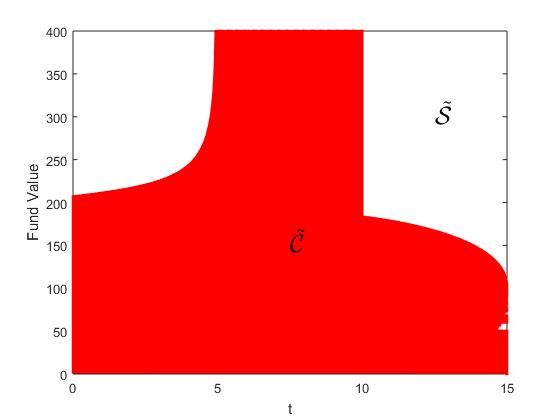
(a) Discontinuous reward function with $c_{1}$	(b) Continuous reward function with $c_{1}$
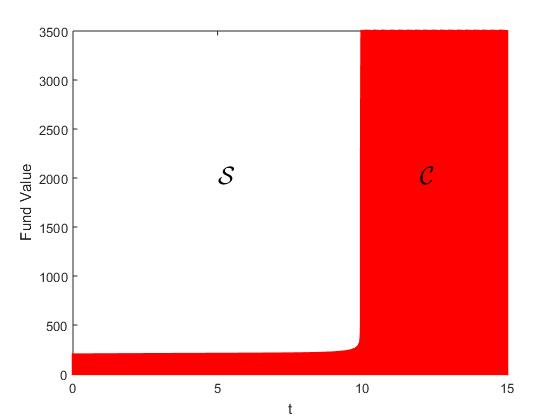
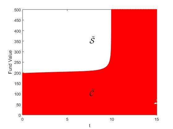
(c) Discontinuous reward function with $c_{2}$	(d) Continuous reward function with $c_{2}$

Figure 1. Comparison of the continuation regions (in red) of the optimal stopping problems with the discontinuous and the continuous reward functions (7) and (14), respectively. The value of the variable annuity contract is approximated using the continuous-time Markov chain approximation described in MacKay et al. (2023). Market and VA parameters are $r=0.03$, $\sigma=0.2$, $F_{0}=G=100$ and $T=15$.

Figure 1 compares the continuation regions (in red) of the two optimal stopping problems, with the discontinuous and the continuous reward functions, in (7) (left panel) and (14) (right panel). We first observe that the surrender regions (in white) are empty between year $5$ and $10$ for the fee function $c_{1}$, and between year $10$ and $15$ for $c_{2}$. This corresponds to the time intervals during which $L(t)>0$, as shown theoretically in Proposition 4.6 (i). Thus, the optimal surrender boundaries of the two problems (left and right panels) are discontinuous when the fee is given by $c_{1}$. It is already known from the literature of variable annuity that the surrender region can have different shapes depending on the fee function, see for example MacKay et al. (2017), Figures 4 and 5. However, such disconnected sets for the surrender region have not been observed in prior numerical work on similar problems, see among others Bernard et al. (2014b), MacKay et al. (2017), Kang and Ziveyi (2018), and MacKay et al. (2023). This simple example illustrates well how different the optimal stopping problem involved in variable annuities pricing differs from the traditional American call and put options often studied in the literature.

Another important feature that is highlighted in the second example (when the fee is modeled by $c_{2}$) is that we no longer have $\lim_{t\rightarrow T}b(t)=G$. This is because the surrender region is empty close to maturity (since $L(t)>0$).

Finally, we observe the two problems, with the discontinuous (left panel) and the continuous (right panel) reward functions, lead to the same continuation and surrender regions, despite the fact that $L(t)<0$ is not satisfied for all $t\in[0,T)$. This indicates that the conditions stated in Proposition 4.9, for the two problems to have the same surrender region, are only sufficient and can be further relaxed. Finding the necessary conditions that make the two optimal stopping problems equivalent is left as future research.

6. Conclusion

In this paper, we perform a rigorous theoretical analysis of the value function involved in the pricing of a variable annuity contract with guaranteed minimum maturity benefit under the Black-Scholes setting with general fee and surrender charge functions. Because of the time dependence, the discontinuity, and the unboundedness of the reward function, many of the standard results in optimal stopping theory do not apply directly to our problem. We show that the optimal stopping problem in (7) admits another representation with a continuous reward function (14), which facilitates the study of the regularity of the value function.

In particular, the continuous reward representation allows us to use existing results from American option pricing theory to obtain the continuity of the value function. We also prove its convexity in the state variable, and its Lipschitz property in $x$ and (locally) in $t$. Then, we derive an integral expression for the early surrender premium, generalizing the results of Bernard et al. (2014a) to general time-dependent fee and surrender charge functions. This second representation of the value function is also known as the early exercise premium representation in the American option pricing literature. From there, we develop a third representation for the value function in terms of the current surrender value and an integral expression that only takes value in the continuation region. We call this third representation the continuation premium representation.

The continuation premium representation turns out to be very helpful in studying the shape of the surrender region. We show that the (non-)emptiness of the surrender region depends on an explicit condition that is expressed solely in terms of the fee and the surrender charge functions. This result is new to the literature and provides a better understanding of the interaction between the fees and the surrender penalty on surrender incentives. When the surrender region is nonempty, we show that $t$-sections of $\mathcal{S}$ are of the form $\mathcal{S}_{t}=[b(t),\infty)$, for some $b(t)\in\mathbb{R}_{+}\cup\{\infty\}$. Investigating the regularity of the optimal surrender boundary theoretically is left as future research.

Disclosure statement

The authors report there are no competing interests to declare.

References

• Alonso-García et al. (2022) J. Alonso-García, M. Sherris, S. Thirurajah, and J. Ziveyi. Taxation and policyholder behavior: the case of guaranteed minimum accumulation benefits. CEPAR Working Paper 2020/17, 2022.
• Bacinello and Zoccolan (2019) A. R. Bacinello and I. Zoccolan. Variable annuities with a threshold fee: valuation, numerical implementation and comparative static analysis. Decisions in Economics and Finance, 42:21–49, 2019.
• Bassan and Ceci (2002) B. Bassan and C. Ceci. Optimal stopping problems with discontinous reward: Regularity of the value function and viscosity solutions. Stochastics and Stochastic Reports, 72(1-2):55–77, 2002.
• Bauer and Moenig (2023) D. Bauer and T. Moenig. Cheaper by the bundle: The interaction of frictions and option exercise in variable annuities. Journal of Risk and Insurance, 90(2):459–486, 2023.
• Bauer et al. (2017) D. Bauer, J. Gao, T. Moenig, E. R. Ulm, and N. Zhu. Policyholder Exercise Behavior in Life Insurance: The State of Affairs. North American Actuarial Journal, 21(4):485–501, 2017.
• Bensoussan and Lions (1982) A. Bensoussan and J.-L. Lions. Applications of Variational Inequalities in Stochastic Control. Noth-Holland Publishing Company, 1982.
• Bernard and MacKay (2015) C. Bernard and A. MacKay. Reducing Surrender Incentives Through Fee Structure in Variable Annuities. In K. Glau, M. Scherer, and R. Zagst, editors, Innovations in Quantitative Risk Management, pages 209–223. Springer, 2015.
• Bernard and Moenig (2019) C. Bernard and T. Moenig. Where Less is More: Reducing Variable Annuity Fees to Benefit Policyholder and Insurer. Journal of Risk and Insurance, 86(3):761–782, 2019.
• Bernard et al. (2014a) C. Bernard, M. Hardy, and A. MacKay. State-Dependent Fees for Variable Annuity Guarantees. ASTIN Bulletin: The Journal of the IAA, 44(3):559–585, 2014a.
• Bernard et al. (2014b) C. Bernard, A. MacKay, and M. Muehlbeyer. Optimal surrender policy for variable annuity guarantees. Insurance: Mathematics and Economics, 55:116–128, 2014b.
• Björk (2009) T. Björk. Arbitrage Theory in Continuous Time. Oxford university press, Third edition, 2009.
• Chiarolla et al. (2022) M. B. Chiarolla, T. De Angelis, and G. Stabile. An analytical study of participating policies with minimum rate guarantee and surrender option. Finance and Stochastics, 26:173–216, 2022.
• Cui et al. (2017) Z. Cui, R. Feng, and A. MacKay. Variable Annuities with VIX-Linked Fee Structure under a Heston-Type Stochastic Volatility Model. North American Actuarial Journal, 21(3):458–483, 2017.
• De Angelis and Stabile (2019) T. De Angelis and G. Stabile. On Lipschitz Continuous Optimal Stopping Boundaries. SIAM Journal on Control and Optimization, 57(1):402–436, 2019.
• Delong (2014) Ł. Delong. Pricing and hedging of variable annuities with state-dependent fees. Insurance: Mathematics and Economics, 58:24–33, 2014.
• El Karoui (1981) N. El Karoui. Les Aspects Probabilistes du Contrôle Stochastique. In P. L. Hennequin, editor, École d’Été de Probabilités de Saint-Flour IX-1979, pages 73–238. Springer, 1981.
• Evans (2010) L. C. Evans. Partial Differential Equations. American Mathematical Society, Second edition, 2010.
• Feng et al. (2022) R. Feng, G. Gan, and N. Zhang. Variable annuity pricing, valuation, and risk management: a survey. Scandinavian Actuarial Journal, 2022(10):867–900, 2022.
• Friedman (1964) A. Friedman. Partial Differential Equations of Parabolic Type. Prentice-Hall, 1964.
• Gao and Ulm (2012) J. Gao and E. R. Ulm. Optimal consumption and allocation in variable annuities with Guaranteed Minimum Death Benefits. Insurance: Mathematics and Economics, 51(3):586–598, 2012.
• Graversen and Peskir (1998) S. E. Graversen and G. Peskir. Optimal stopping and maximal inequalities for geometric Brownian motion. Journal of Applied Probability, 35(4):856–872, 1998.
• Jacka (1991) S. D. Jacka. Optimal Stopping and the American Put. Mathematical Finance, 1(2):1–14, 1991.
• Jacka (1993) S. D. Jacka. Local Times, Optimal Stopping and Semimartingales. The Annals of Probability, 21(1):329–339, 1993.
• Jacka and Lynn (1992) S. D. Jacka and J. R. Lynn. Finite-horizon optimal stopping, obstacle problems and the shape of the continuation region. Stochastics and Stochastic Reports, 39(1):25–42, 1992.
• Jaillet et al. (1990) P. Jaillet, D. Lamberton, and B. Lapeyre. Variational inequalities and the pricing of American options. Acta Applicandae Mathematica, 21:263–289, 1990.
• Jeon and Kwak (2018) J. Jeon and M. Kwak. Optimal surrender strategies and valuations of path-dependent guarantees in variable annuities. Insurance: Mathematics and Economics, 83:93–109, 2018.
• Jönsson et al. (2006) H. Jönsson, A. G. Kukush, and D. S. Silvestrov. Threshold structure of optimal stopping strategies for American type option. II. Theory of Probability and Mathematical Statistics, 72:47–58, 2006.
• Kang and Ziveyi (2018) B. Kang and J. Ziveyi. Optimal surrender of guaranteed minimum maturity benefits under stochastic volatility and interest rates. Insurance: Mathematics and Economics, 79:43–56, 2018.
• Karatzas and Shreve (1991) I. Karatzas and S. E. Shreve. Brownian Motion and Stochastic Calculus. Springer-Verlag, Second edition, 1991.
• Karatzas and Shreve (1998) I. Karatzas and S. E. Shreve. Methods of Mathematical Finance. Springer, 1998.
• Kirkby and Aguilar (2023) J. L. Kirkby and J.-P. Aguilar. Valuation and optimal surrender of variable annuities with guaranteed minimum benefits and periodic fees. Scandinavian Actuarial Journal, 2023(6):624–654, 2023.
• Kotlow (1973) D. B. Kotlow. A free boundary problem connected with the optimal stopping problem for diffusion processes. Transactions of the American Mathematical Society, 184:457–478, 1973.
• Kouritzin and MacKay (2018) M. A. Kouritzin and A. MacKay. VIX-linked fees for GMWBs via explicit solution simulation methods. Insurance: Mathematics and Economics, 81:1–17, 2018.
• Krylov (1980) N. V. Krylov. Controlled Diffusion Processes. Springer, 1980.
• Ladyz̆enskaja et al. (1968) O. A. Ladyz̆enskaja, V. A. Solonnikov, and N. N. Ural’ceva. Linear and Quasi-linear Equations of Parabolic Type. American Mathematical Society, 1968.
• Lamberton (1998) D. Lamberton. American options. In D. J. Hand and S. D. Jacka, editors, Statistic in Finance. Arnold, 1998.
• Lamberton (2009) D. Lamberton. Optimal stopping and American options. Ljubljana Summer School on Financial Mathematics, September 2009.
• Luo and Xing (2021) X. Luo and J. Xing. Optimal Surrender Policy of Guaranteed Minimum Maturity Benefits in Variable Annuities with Regime-Switching Volatility. Mathematical Problems in Engineering, 2021:1–20, 2021.
• MacKay (2014) A. MacKay. Fee Structure and Surrender Incentives in Variable Annuities. PhD thesis, University of Waterloo, August 2014.
• MacKay et al. (2017) A. MacKay, M. Augustyniak, C. Bernard, and M. R. Hardy. Risk Management of Policyholder Behavior in Equity-Linked Life Insurance. Journal of Risk and Insurance, 84(2):661–690, 2017.
• MacKay et al. (2023) A. MacKay, M.-C. Vachon, and Z. Cui. Analysis of VIX-linked fee fncentives in variable annuities via continuous-time Markov chain approximation. Quantitative Finance, 23(7-8):1055–1078, 2023.
• Milevsky and Salisbury (2001) M. A. Milevsky and T. S. Salisbury. The Real Option to Lapse a Variable Annuity: Can Surrender Charges Complete the Market? In Conference Proceedings of the 11th Annual International AFIR Colloquium, 2001.
• Moenig and Bauer (2016) T. Moenig and D. Bauer. Revisiting the Risk-Neutral Approach to Optimal Policyholder Behavior: A Study of Withdrawal Guarantees in Variable Annuities. Review of Finance, 20(2):759–794, 2016.
• Moenig and Zhu (2018) T. Moenig and N. Zhu. Lapse-and-Reentry in Variable Annuities. Journal of Risk and Insurance, 85(4):911–938, 2018.
• Moenig and Zhu (2021) T. Moenig and N. Zhu. The Economics of a Secondary Market for Variable Annuities. North American Actuarial Journal, 25(4):604–630, 2021.
• Niittuinperä (2022) J. Niittuinperä. Chapter 18— Policyholder Behavior and Management Actions. In IAA Risk Book. 2022.
• Palczewski and Stettner (2010) J. Palczewski and Ł. Stettner. Finite Horizon Optimal Stopping of Time-Discontinuous Functionals with Applications to Impulse Control with Delay. SIAM Journal on Control and Optimization, 48(8):4874–4909, 2010.
• Palmer (2006) B. A. Palmer. Equity-Indexed Annuities: Fundamental Concepts and Issues. Technical report, Insurance Information Institute, 2006.
• Peskir and Shiryaev (2006) G. Peskir and A. Shiryaev. Optimal Stopping and Free-Boundary Problems. Birkhäuser Basel, 2006.
• Rudin (1991) W. Rudin. Functional Analysis. McGraw-Hill, Inc., Second edition, 1991.
• Terenzi (2019) G. Terenzi. Option prices in stochastic volatility models. PhD thesis, Università di Roma Tor Vergata and Université Paris-Est Marne-La-Vallée, 2019.
• Van Moerbeke (1974) P. Van Moerbeke. Optimal Stopping and Free Boundary Problems. The Rocky Mountain Journal of Mathematics, 4(3):539–578, 1974.
• Veretennikov (1981) A. J. Veretennikov. On Strong Solutions and Explicit Formulas for Solutions of Stochastic Integral Equations. Mathematics of the USSR-Sbornik, 39(3):387–403, 1981.
• Villeneuve (1999) S. Villeneuve. Exercise regions of American options on several assets. Finance and Stochastics, 3:295–322, 1999.
• Villeneuve (2007) S. Villeneuve. On Threshold Strategies and the Smooth-Fit Principle for Optimal Stopping Problems. Journal of Applied Probability, 44(1):181–198, 2007.
• Zhu and Welsch (2015) Z. Zhu and R. E. Welsch. Statistical learning for variable annuity policyholder withdrawal behavior. Applied Stochastic Models in Business and Industry, 31(2):137–147, 2015.