Type II Hamiltonian Lie Group Variational Integrators with Applications to Geometric Adjoint Sensitivity Analysis

Abstract.

Variational integrators for Euler–Lagrange equations and Hamilton’s equations are a class of structure-preserving numerical methods that respect the conservative properties of such systems. Lie group variational integrators are a particular class of these integrators that apply to systems which evolve over the tangent bundle and cotangent bundle of Lie groups. Traditionally, these are constructed from a variational principle which assumes fixed position endpoints. In this paper, we instead construct Lie group variational integrators with a novel Type II variational principle on the cotangent bundle of a Lie group which allows for Type II boundary conditions, i.e., fixed initial position and final momenta; these boundary conditions are particularly important for adjoint sensitivity analysis, which is the motivating application in our paper. In general, such Type II variational principles are only globally defined on vector spaces or locally defined on general manifolds; however, by left translation, we are able to define this variational principle globally on cotangent bundles of Lie groups. By developing the continuous and discrete Type II variational principles over Lie groups, we construct a structure-preserving Lie group variational integrator that is both symplectic and momentum-preserving. Subsequently, we introduce adjoint systems on Lie groups, and show how these adjoint systems can be used to perform geometric adjoint sensitivity analysis for optimization problems on Lie groups. Finally, we conclude with two numerical examples to show how adjoint sensitivity analysis can be used to solve initial-value optimization problems and optimal control problems on Lie groups.

1. Introduction

In this paper, we aim to develop Lie group variational integrators from a Type II variational principle with the motivating application of performing intrinsic geometric adjoint sensitivity analysis on Lie groups. Lie Group variational integrators are a class of geometric structure-preserving integrators for integrating Lagrangian or Hamiltonian systems evolving over tangent and cotangent bundles of Lie groups (see [27; 28; 26; 5; 37; 34; 23]). Such methods generally have good conservation properties, such as respecting the symplecticity and momentum-preservation of these systems. Adjoint systems provide an efficient method for performing dynamically-constrained optimization and sensitivity analysis. The geometry of these systems has gained interest as it can be described by a Hamiltonian structure. Particularly, the Hamiltonian structure of adjoint systems encode a quadratic conservation law which is the key to adjoint sensitivity analysis [44]. We aim to synthesize these two areas of research, by developing Lie group variational integrators which are applicable to the maximally degenerate Hamiltonian structures found in adjoint systems and hence, develop geometric integrators which respect the quadratic conservation law enjoyed by adjoint systems, making them particularly useful for adjoint sensitivity analysis on Lie groups. We begin with a brief introduction and review of these topics.

1.1. Lagrangian and Hamiltonian Variational Integrators

Geometric numerical integration aims to preserve geometric conservation laws under discretization, and this field is surveyed in the monograph by Hairer et al. [18]. Discrete variational mechanics [36; 30] provides a systematic method of constructing symplectic integrators. It is typically approached from a Lagrangian perspective by introducing the discrete Lagrangian, $L_{d}:Q\times Q\rightarrow\mathbb{R}$, which is a Type I generating function of a symplectic map and approximates the exact discrete Lagrangian, which is constructed from the Lagrangian $L:TQ\rightarrow\mathbb{R}$ as

(1.1) $$L_{d}^{E}(q_{0},q_{1};h)=\operatorname{ext}_{\begin{subarray}{c}q\in C^{2}([0,h],Q)\\ q(0)=q_{0},q(h)=q_{1}\end{subarray}}\int_{0}^{h}L(q(t),\dot{q}(t))dt,$$

which is equivalent to Jacobi’s solution of the Hamilton–Jacobi equation. The exact discrete Lagrangian generates the exact discrete-time flow map of a Lagrangian system, but, in general, it cannot be computed explicitly. Instead, this can be approximated by replacing the integral with a quadrature formula, and replacing the space of $C^{2}$ curves with a finite-dimensional function space.

Given a finite-dimensional function space $\mathbb{M}^{n}([0,h])\subset C^{2}([0,h],Q)$ and a quadrature formula $\mathcal{G}:C^{2}([0,h],Q)\rightarrow\mathbb{R}$, $\mathcal{G}(f)=h\sum_{j=1}^{m}b_{j}f(c_{j}h)\approx\int_{0}^{h}f(t)dt$, the Galerkin discrete Lagrangian is

$$L_{d}(q_{0},q_{1})=\operatorname{ext}_{\begin{subarray}{c}q\in\mathbb{M}^{n}([0,h])\\ q(0)=q_{0},q(h)=q_{1}\end{subarray}}\mathcal{G}(L(q,\dot{q}))=\operatorname{ext}_{\begin{subarray}{c}q\in\mathbb{M}^{n}([0,h])\\ q(0)=q_{0},q(h)=q_{1}\end{subarray}}h\sum\nolimits_{j=1}^{m}b_{j}L(q(c_{j}h),\dot{q}(c_{j}h)).$$

Given a discrete Lagrangian $L_{d}$, the discrete Hamilton–Pontryagin principle imposes the discrete second-order condition $q_{k}^{1}=q_{k+1}^{0}$ using Lagrange multipliers $p_{k+1}$, which yields a variational principle on $(Q\times Q)\times_{Q}T^{*}Q$,

$$\delta\left[\sum\nolimits_{k=0}^{n-1}L_{d}(q_{k}^{0},q_{k}^{1})+\sum\nolimits_{k=0}^{n-2}p_{k+1}(q_{k+1}^{0}-q_{k}^{1})\right]=0.$$

This in turn yields the implicit discrete Euler–Lagrange equations,

(1.2) $$q_{k}^{1}=q_{k+1}^{0},\qquad p_{k+1}=D_{2}L_{d}(q_{k}^{0},q_{k}^{1}),\qquad p_{k}=-D_{1}L_{d}(q_{k}^{0},q_{k}^{1}),$$

where $D_{i}$ denotes the partial derivative with respect to the $i$-th argument. Making the identification $q_{k}=q_{k}^{0}=q_{k-1}^{1}$, we obtain the discrete Lagrangian map and discrete Hamiltonian map which are $F_{L_{d}}:(q_{k-1},q_{k})\mapsto(q_{k},q_{k+1})$ and $\tilde{F}_{L_{d}}:(q_{k},p_{k})\mapsto(q_{k+1},p_{k+1})$, respectively. The last two equations of (1.2) define the discrete fiber derivatives, $\mathbb{F}L_{d}^{\pm}:Q\times Q\rightarrow T^{*}Q$,

$$\mathbb{F}L_{d}^{+}(q_{k},q_{k+1}) =(q_{k+1},D_{2}L_{d}(q_{k},q_{k+1})),$$

$$\mathbb{F}L_{d}^{-}(q_{k},q_{k+1}) =(q_{k},-D_{1}L_{d}(q_{k},q_{k+1})).$$

These two discrete fiber derivatives induce a single unique discrete symplectic form $\Omega_{L_{d}}=(\mathbb{F}L_{d}^{\pm})^{*}\Omega$, where $\Omega$ is the canonical symplectic form on $T^{*}Q$, and the discrete Lagrangian and Hamiltonian maps preserve $\Omega_{L_{d}}$ and $\Omega$, respectively. The discrete Lagrangian and Hamiltonian maps can be expressed as $F_{L_{d}}=(\mathbb{F}L_{d}^{-})^{-1}\circ\mathbb{F}L_{d}^{+}$ and $\tilde{F}_{L_{d}}=\mathbb{F}L_{d}^{+}\circ(\mathbb{F}L_{d}^{-})^{-1}$, respectively. This characterization allows one to relate the approximation error of the discrete flow maps to the approximation error of the discrete Lagrangian.

The variational integrator approach simplifies the numerical analysis of symplectic integrators. The task of establishing the geometric conservation properties and order of accuracy of the discrete Lagrangian map $F_{L_{d}}$ and discrete Hamiltonian map $\tilde{F}_{L_{d}}$ reduces to the simpler task of verifying certain properties of the discrete Lagrangian $L_{d}$ instead.

Theorem 1.1 (Discrete Noether’s theorem (Theorem 1.3.3 of [36])).

If a discrete Lagrangian $L_{d}$ is invariant under the diagonal action of $G$ on $Q\times Q$, then the single unique discrete momentum map, $\mathbf{J}_{L_{d}}=(\mathbb{F}L_{d}^{\pm})^{*}\mathbf{J}$, is invariant under the discrete Lagrangian map $F_{L_{d}}$, i.e., $F_{L_{d}}^{*}\mathbf{J}_{L_{d}}=\mathbf{J}_{L_{d}}$.

Theorem 1.2 (Variational error analysis (Theorem 2.3.1 of [36])).

If a discrete Lagrangian $L_{d}$ approximates the exact discrete Lagrangian $L_{d}^{E}$ to order $p$, i.e., $L_{d}(q_{0},q_{1};h)=L_{d}^{E}(q_{0},q_{1};h)+\mathcal{O}(h^{p+1}),$ then the discrete Hamiltonian map $\tilde{F}_{L_{d}}$ is an order $p$ accurate one-step method.

The bounded energy error of variational integrators can be understood by performing backward error analysis, which then shows that the discrete flow map is approximated with exponential accuracy by the exact flow map of the Hamiltonian vector field of a modified Hamiltonian [3; 47].

Given a degenerate Hamiltonian, where the Legendre transform $\mathbb{F}H:T^{*}Q\rightarrow TQ$, $(q,p)\mapsto(q,\frac{\partial H}{\partial p})$, is noninvertible, there is no equivalent Lagrangian formulation. Thus, a characterization of variational integrators directly in terms of the continuous Hamiltonian is desirable. This is achieved by considering the Type II analogue of Jacobi’s solution, given by

$$H_{d}^{+,E}(q_{k},p_{k+1})=\operatorname{ext}_{\begin{subarray}{c}(q,p)\in C^{2}([t_{k},t_{k+1}],T^{*}Q)\\ q(t_{k})=q_{k},p(t_{k+1})=p_{k+1}\end{subarray}}\Big{[}p(t_{k+1})q(t_{k+1})-\int_{t_{k}}^{t_{k+1}}\left[p\dot{q}-H(q,p)\right]dt\Big{]}.$$

A computable Galerkin discrete Hamiltonian $H_{d}^{+}$ is obtained by choosing a finite-dimensional function space and a quadrature formula,

$$H_{d}^{+}(q_{0},p_{1})=\operatorname{ext}_{\begin{subarray}{c}q\in\mathbb{M}^{n}([0,h])\\ q(0)=q_{0}\\ (q(c_{j}h),p(c_{j}h))\in T^{*}Q\end{subarray}}\left[p_{1}q(t_{1})-h\sum\nolimits_{j=1}^{m}b_{j}[p(c_{j}h)\dot{q}(c_{j}h)-H(q(c_{j}h),p(c_{j}h))]\right].$$

Interestingly, the Galerkin discrete Hamiltonian does not require a choice of a finite-dimensional function space for the curves in the momentum, as the quadrature approximation of the action integral only depend on the momentum values $p(c_{j}h)$ at the quadrature points, which are determined by the extremization principle. In essence, this is because the action integral does not depend on the time derivative of the momentum $\dot{p}$. As such, both the Galerkin discrete Lagrangian and the Galerkin discrete Hamiltonian depend only on the choice of a finite-dimensional function space for curves in the position, and a quadrature rule. It was shown in Proposition 4.1 of [31] that when the Hamiltonian is hyperregular, and for the same choice of function space and quadrature rule, they induce equivalent numerical methods.

The Type II discrete Hamilton’s phase space variational principle states that

$$\delta\left\{p_{N}q_{N}-\sum_{k=0}^{N-1}\left[p_{k+1}q_{k+1}-H_{d}^{+}(q_{k},p_{k+1})\right]\right\}=0,$$

for discrete curves in $T^{*}Q$ with fixed $(q_{0},p_{N})$ boundary conditions. This yields the discrete Hamilton’s equations, which are given by

(1.3) $$q_{k+1}=D_{2}H_{d}^{+}(q_{k},p_{k+1}),\qquad p_{k}=D_{1}H_{d}^{+}(q_{k},p_{k+1}).$$

Given a discrete Hamiltonian $H_{d}^{+}$, we introduce the discrete fiber derivatives (or discrete Legendre transforms), $\mathbb{F}^{+}H_{d}^{+}$,

$$\mathbb{F}^{+}H_{d}^{+} :(q_{0},p_{1})\mapsto(D_{2}H_{d}^{+}(q_{0},p_{1}),p_{1}),$$

$$\mathbb{F}^{-}H_{d}^{+} :(q_{0},p_{1})\mapsto(q_{0},D_{1}H_{d}^{+}(q_{0},p_{1})).$$

The discrete Hamiltonian map can be expressed in terms of the discrete fiber derivatives,

$$\tilde{F}_{H_{d}^{+}}(q_{0},p_{0})=\mathbb{F}^{+}H_{d}^{+}\circ(\mathbb{F}^{-}H_{d}^{+})^{-1}(q_{0},p_{0})=(q_{1},p_{1}),$$

Similar to the Lagrangian case, we have a discrete Noether’s theorem and variational error analysis result for Hamiltonian variational integrators.

Theorem 1.3 (Discrete Noether’s theorem (Theorem 5.3 of [31])).

Given the action $\Phi$ on the configuration manifold $Q$, let $\Phi^{T^{*}Q}$ be the cotangent lifted action on $T^{*}Q$. If the generalized discrete Lagrangian $R_{d}(q_{0},q_{1},p_{1})=p_{1}q_{1}-H_{d}^{+}(q_{0},p_{1})$ is invariant under the cotangent lifted action $\Phi^{T^{*}Q}$, then the discrete Hamiltonian map $\tilde{F}_{H_{d}^{+}}$ preserves the momentum map, i.e., $\tilde{F}_{H_{d}^{+}}^{*}\mathbf{J}=\mathbf{J}$.

Theorem 1.4 (Variational error analysis (Theorem 2.2 of [45])).

If a discrete Hamiltonian $H_{d}^{+}$ approximates the exact discrete Hamiltonian $H_{d}^{+,E}$ to order $p$, i.e., $H_{d}^{+}(q_{0},p_{1};h)=H_{d}^{+,E}(q_{0},p_{1};h)+\mathcal{O}(h^{p+1})$, then the discrete Hamiltonian map $\tilde{F}_{H_{d}^{+}}$ is an order $p$ accurate one-step method.

It should be noted that there is an analogous theory of discrete Hamiltonian variational integrators based on Type III generating functions $H_{d}^{-}(p_{0},q_{1})$.

Remark 1.1.

It should be noted that the current construction of Hamiltonian variational integrators is only valid on vector spaces and local coordinate charts as it involves Type II/Type III generating functions $H_{d}^{+}(q_{k}.p_{k+1})$, $H_{d}^{-}(p_{k},q_{k+1})$, which depend on the position at one boundary point, and the momentum at the other boundary point. However, this does not make intrinsic sense on a manifold, since one needs the base point in order to specify the corresponding cotangent space. One possible approach to constructing an intrinsic formulation of Hamiltonian variational integrators on general cotangent bundles is to start with discrete Dirac mechanics [30], and consider a generating function $E_{d}^{+}(q_{k},q_{k+1},p_{k+1})$, $E_{d}^{-}(q_{k},p_{k},q_{k+1})$, that depends on the position at both boundary points and the momentum at one of the boundary points. This approach can be viewed as a discretization of the generalized energy $E(q,v,p)=\langle p,v\rangle-L(q,v)$, in contrast to the Hamiltonian $H(q,p)=\operatorname{ext}_{v}\langle p,v\rangle-L(q,v)=\left.\langle p,v\rangle-L(q,v)\right|_{p=\frac{\partial L}{\partial v}}$.

As mentioned in the previous remark, an issue with Type II Hamiltonian variational integrators is that they are only valid on vector spaces or on local charts, due to the Type II boundary conditions $q(t_{k})=q_{k},p(t_{k+1})=p_{k+1}$, which requires a local trivialization of $T^{*}Q$. Furthermore, these methods cannot in general be extended to arbitrary parallelizable manifolds $M$, i.e., $T^{*}M\cong M\times V$ for some vector space $V$, since the isomorphism $T^{*}M\cong M\times V$ may be neither explicit nor computable. However, for a Lie group $G$, the trivialization $T^{*}G\cong G\times\mathfrak{g}^{*}$ is given simply by left or right translation. Using this trivialization, we will extend the construction of Type II Hamiltonian variational integrators to the setting of Hamiltonian systems on the cotangent bundle of a Lie group.

1.2. Lie Group Variational Integrators

Lie group variational integrators preserve the Lie group structure of the configuration space without the use of local charts, reprojection, or constraints. Instead, the discrete solution is updated using the exponential of a Lie algebra element that satisfies a discrete variational principle. These yield highly efficient geometric integration schemes for rigid body dynamics that automatically remain on the rotation group. We avoid coordinate singularities associated with local charts, such as Euler angles, by representing the attitude globally as a rotation matrix, which is important for accurately simulating chaotic orbital motion.

These ideas were introduced in [26], and applied to a system of extended rigid bodies interacting under their mutual gravitational potential in [27; 28], wherein symmetry reduction to a relative frame is also addressed. The superior computational efficiency of Lie group variational integrators for the full body simulation of systems of extended rigid bodies in the context of astrodynamics was demonstrated in [15].

Lie group variational integrators can be seen as the synthesis of Lie group methods (see, for example, [22]) and variational integrators that serves as the basis for constructing efficient geometric structure-preserving integrators for the dynamics of mechanical systems which evolve on Lie groups.

The basic idea of a Lie group method is to express the solution in terms of an element of the Lie algebra,

$$g(t)=g_{0}\exp(\xi(t))\,,$$

as opposed to a group element, and to use the exponential map and group composition to ensure that the solution remains on the group. The problem reduces to finding an appropriate Lie algebra element $\xi\in\mathfrak{g}$, which is desirable, as the Lie algebra is always linear, even when the Lie group is nonlinear, and interpolants can be easily obtained. We construct an interpolant on the Lie group by using polynomial interpolation at the level of the Lie algebra.

The exponential (or an approximation thereof, such as the Cayley transform, or more generally, the diagonal Padé approximants, for quadratic matrix Lie groups [9]) allows one to approximate a curve on $G$ by a discrete time curve on the Lie algebra. One can combine this with an approximation space for the fibers of $TG\cong G\times\mathfrak{g}$ to obtain a discrete Lagrangian. Enforcing a discrete variational principle then results in a Lie group variational integrator. For more details, see [27; 28; 26; 5; 37; 34; 23].

1.3. Adjoint Systems and their Geometry

The solution of many nonlinear problems involves successive linearization, and as such variational equations and their adjoints play a critical role in a variety of applications. Adjoint equations are of particular interest when the parameter space has significantly higher dimension than that of the output or objective. In particular, the simulation of adjoint equations arise in sensitivity analysis [7; 8], adaptive mesh refinement [33], uncertainty quantification [51], automatic differentiation [17], superconvergent functional recovery [41], optimal control [42], optimal design [16], optimal estimation [40], and deep learning viewed as an optimal control problem [4].

The study of geometric aspects of adjoint systems arose from the observation that the combination of any system of differential equations and its adjoint equations are described by a formal Lagrangian [20; 21]. This naturally leads to the question of when the formation of adjoints and discretization commutes [46], and prior work on this include the Ross–Fahroo lemma [43], and the observation by Sanz-Serna [44] that the adjoints and discretization commute if and only if the discretization is symplectic.

We will briefly review the geometry of adjoint and variational systems. Let $M$ be a manifold; throughout this paper, we will assume that all manifolds are smooth and finite-dimensional and all maps between them are smooth, unless otherwise stated. Let $\dot{q}=F(q)$ be an ODE on $M$, specified by a vector field $F$ on $M$. Then, the adjoint system associated to $F$ is the ODE on $T^{*}M$ with the coordinate expression

$$\dot{q} =F(q),$$

$$\dot{p} =-[DF(q)]^{*}p,$$

where $DF$ is the linearization of $F$. The adjoint system can be viewed as the ODE on $T^{*}M$ corresponding to the vector field given by the cotangent lift of $F$. Intrinsically, the adjoint system can be understood as a Hamiltonian system on $T^{*}M$ relative to the canonical symplectic form on $T^{*}M$, with Hamiltonian given by

$$H(q,p)=\langle p,F(q)\rangle.$$

Furthermore, we associate to $F$ the variational system, which is the ODE on $TM$ with coordinate expression

$$\dot{q} =F(q),$$

$$\dot{v} =DF(q)v.$$

The variational system can be viewed as the ODE on $TM$ corresponding to the vector field given by the tangent lift of $F$.

The importance of the adjoint and variational systems is that they satisfy an adjoint-variational quadratic conservation law: for any solution curves $(q,p)$ of the adjoint system and $(q,v)$ of the variational system, covering the same base curve $q$, one has

$$\frac{d}{dt}\langle p,v\rangle=0.$$

This quadratic conservation law is the key to adjoint sensitivity analysis [44]. The interest in studying the geometry of these adjoint and variational systems arises from the fact that this quadratic conservation law can also be interpreted as symplecticity of the Hamiltonian flow of the adjoint system [49].

In [49], we developed Type II variational integrators for adjoint systems for ODEs and DAEs on vector spaces by utilizing their respective symplectic and presymplectic structures. One of the goals of this paper is to extend this construction to the nonlinear setting and in particular, adjoint systems over Lie groups.

1.4. Main Contributions

In this paper, we develop a continuous and discrete theory for Type II variational principles on cotangent bundles of Lie groups, which gives an intrinsic meaning to Hamiltonian systems with fixed initial position $g_{0}$ and fixed terminal momenta $p_{1}$ boundary conditions, in contrast to traditional variational principles for Lie group variational integrators which assume fixed initial and final positions. The motivation for developing Type II variational principles is that the corresponding Type II boundary conditions arise in adjoint sensitivity analysis, which is the motivating application of this paper. Traditionally, such Type II variational principles are only globally defined on vector spaces, or locally defined on charts on a general manifold; however, for Lie groups, left-trivialization allows us to define such a Type II variational principle globally on the cotangent bundle of a Lie group. Specifically, in Section 2, we develop a novel Type II variational principle for Hamiltonian systems on cotangent bundles of Lie groups by introducing a d’Alembert variational principle. This is a novel variational principle since typically, variational principles are given by a stationarity condition for the action corresponding to fixed initial and terminal positions, $g_{0}$ and $g_{1}$; however, in our setting, since the final position $g_{1}$ is not fixed, virtual work can be deposited into the system by varying $g_{1}$. This is accounted for in our variational principle by demanding that the action is stationary only modulo this virtual work term arising from $g_{1}$ boundary variations. Subsequently, we discretize the variational principle to develop structure-preserving numerical methods for such systems. We prove that such methods are symplectic and also momentum-preserving. We also develop a discrete reduction theory for left-invariant systems, and show that the discrete reduction theory can be interpreted as momentum preservation associated to left-invariance.

In Section 3, we apply the continuous and discrete theory developed in Section 2 to the particular case of adjoint Hamiltonian systems on Lie groups. In the continuous setting, we introduce the adjoint and variational equations associated to an ODE on a Lie group, and prove global existence and uniqueness results for these equations. In the discrete setting, we show how our variational integrators can be used to perform intrinsic structure-preserving adjoint sensitivity analysis on Lie groups. In particular, we show how initial condition sensitivities and parameter sensitivities of cost functions can be computed exactly within this framework. Finally, we conclude with two numerical examples, which utilizes this geometric adjoint sensitivity analysis to solve an initial condition optimization problem and an optimal control problem on $SO(3)$.

2. Hamiltonian Variational Integrators on Cotangent Bundles of Lie Groups

In this paper, we aim to construct and analyze geometric integration methods for Hamiltonian dynamics on the cotangent bundle $T^{*}G$ of a Lie group $G$, subject to Type II boundary conditions $g(0)=g_{0},p(T)=p_{1}$. Throughout, our our motivating class of examples is adjoint systems.

Example 2.1 (Adjoint Systems on Lie Groups).

Consider an ODE on a Lie group $G$ given by $\dot{g}=f(g)$, specified by a vector field $F$ on $G$. We associate to $F$ the adjoint Hamiltonian $H:T^{*}G\rightarrow\mathbb{R}$, given by

$$H(g,p)=\langle p,F(q)\rangle.$$

We refer to the Hamiltonian system $i_{X_{H}}\Omega=dH$, relative to the canonical symplectic form $\Omega$ on $T^{*}G$, as the adjoint system associated to the ODE $\dot{g}=F(g)$. The motivation for considering Type II boundary conditions arises from the fact that, viewing the ODE on $G$ as flowing forward in time, the momenta $p$ can be interpreted as flowing backward in time, which backpropagates sensitivity information back to the initial time. We will describe this in more detail in Section 3.

We also provide as another motivating example the class of mechanical systems on $T^{*}G$. Although we will not be particularly concerned with this class of examples in this paper, it is worthwhile pointing out the distinctions between these two classes of examples (see Remark 2.1).

Example 2.2 (Mechanical Systems on $TG$).

We consider a mechanical system on a Lie group $G$ described by a Lagrangian $L:TG\rightarrow\mathbb{R}$. By left-trivialization of the tangent bundle,

$$TG\ni(g,\dot{g})\mapsto(g,\xi)=(g,g^{-1}\dot{g})\in G\times\mathfrak{g},$$

the Euler–Lagrange equations for $l(g,\xi)\equiv L(g,g\xi)$ can be expressed as

$$\frac{d}{dt}\frac{\delta l}{\delta\xi} =\text{ad}^{*}_{\xi}\frac{\delta l}{\delta\xi}+d_{g}l,$$

$$\frac{d}{dt}g =g\xi.$$

Assuming that the Lagrangian is hyperregular, i.e., $\mathbb{F}L:TG\rightarrow T^{*}G$ is a diffeomorphism, the system can be equivalently described as a Hamiltonian system on $T^{*}G$; or by left-trivialization, it can be equivalently described as a Hamiltonian system on $G\times\mathfrak{g}^{*}\ni(g,\mu)$ given by

$$\frac{d}{dt}\mu =\text{ad}_{\xi}^{*}\mu+g\frac{\delta l}{\delta g},$$

$$\frac{d}{dt}g =\xi,$$

$$\mu =\frac{\delta l}{\delta\xi}.$$

For more details on this class of examples, see [5; 6; 23].

Remark 2.1.

It is interesting to note that these two classes of examples, Example 2.1 and Example 2.2, are at the opposing ends of the spectrum of regularity and degeneracy for Hamiltonian systems.

Recall that a Hamiltonian is said to be regular if the Hessian of the Hamiltonian $D^{2}_{p}H(q,p)$ is invertible for all $(q,p)\in T^{*}G$ and degenerate otherwise. If the Hamiltonian is regular, then the (inverse) Legendre transform $\mathbb{F}H:T^{*}G\rightarrow TG$ is a local diffeomorphism.

On the one hand, systems of the form described in Example 2.2 are regular and furthermore, they are maximally regular (or hyperregular) in the sense that $\mathbb{F}H:T^{*}G\rightarrow TG$ is a global diffeomorphism.

On the other hand, adjoint systems of the form described in Example 2.1 are maximally degenerate, in the sense that the Hessian $D^{2}_{p}H(q,p)$ is the zero matrix. While this appears to be a deficiency of such systems, we will see that this is a key property of these systems, arising from the fact that these systems are lifts of differential equations on the base space $G$.

Because adjoint systems are degenerate, they do not admit an equivalent Lagrangian description. As such, we aim to construct integrators for Hamiltonian systems on $T^{*}G$ without assuming that they arise from a Lagrangian system.

2.1. A Type II Variational Principle for Hamiltonian Systems on Cotangent Bundles of Lie Groups

A common approach to constructing geometric integrators for Lagrangian and Hamiltonian systems is to restrict the variational principle, from which these systems arise, to some appropriate finite-dimensional space of possible trajectories, and solve the approximate problem on this restricted space. We thus aim to construct integrators for Hamiltonian systems on $T^{*}G$ by first formulating a variational principle for these systems in the continuous setting and subsequently restricting to a discrete variational principle.

To develop a variational principle for Hamiltonian systems on $T^{*}G$, we first consider the boundary conditions that we wish to place on the system. Note that fixed endpoint conditions on the basespace $g(0)=g_{0},g(T)=g_{1}$ are generally incompatible with systems of the form Example 2.1, since adjoint systems on $T^{*}G$ cover first-order ODEs on $G$ and thus, one cannot freely specify both $g(0)$ and $g(T)$. As such, we instead consider Type II boundary conditions of the form $g(0)=g_{0},p(T)=p_{1}$. For general Hamiltonian systems on the cotangent bundle of a manifold, the issue with these boundary conditions is that one cannot intrinsically specify a covector $p(T)=p_{1}$ without specifying the basepoint $q(T)=q_{1}$. This is not an issue for adjoint systems in particular, since the time-$T$ flow of the underlying ODE on $G$ determines the basepoint where $p_{1}$ is specified. However, since we would like our theory to apply to general Hamiltonian systems on $T^{*}G$, we do not want to restrict to adjoint systems in particular. Fortunately, we can make sense of Type II boundary conditions, since $T^{*}G$ is trivializable by left-translation.

Let $\mathfrak{g}=T_{e}G$ denote the Lie algebra of $G$ and $\mathfrak{g}^{*}=T^{*}_{e}G$ be its dual. We will denote the duality pairing between $v\in T_{g}G$ and $p\in T_{g}^{*}G$ as $\langle p,v\rangle$, where the base point is understood in context. Let $L_{g}:G\rightarrow G$ denote left-translation by $g$, $L_{g}(x)=gx$. Left-translation induces maps on the tangent bundle and cotangent bundle of $G$ by pushforward and pullback, respectively, which we denote as

$$T_{x}L_{g} :T_{x}G\rightarrow T_{gx}G,$$

$$T_{x}^{*}L_{g} :T_{gx}^{*}G\rightarrow T_{x}^{*}G.$$

For $v_{g}\in T_{g}G,p_{g}\in T_{g}^{*}G$, we will denote their left-translations to their respective fibers over the identity as simply

$$g^{-1}v_{g} \equiv T_{g}L_{g^{-1}}(v_{g})\in\mathfrak{g},$$

$$g^{*}p_{g} \equiv T^{*}_{e}L_{g}(p_{g})\in\mathfrak{g}^{*}.$$

This notation is suggestive, since in the case that $G$ is a matrix Lie group, the left-translation of a tangent vector to the fiber over the identity acts by matrix multiplication by the inverse of $g$ and the left-translation of a covector to the fiber over the identity acts by matrix multiplication by the adjoint of $g$.

A useful fact is that the pairing $\langle p_{g},v_{g}\rangle$ is preserved under left-translation,

$$\langle g^{*}\cdot p_{g},g^{-1}\cdot v_{g}\rangle =\langle T_{e}^{*}L_{g}(p_{g}),T_{g}L_{g^{-1}}(v_{g})\rangle$$

$$=\langle p_{g},T_{e}L_{g}\circ T_{g}L_{g^{-1}}(v_{g})\rangle$$

$$=\langle p_{g},T_{g}(L_{g}\circ L_{g^{-1}})(v_{g})\rangle$$

$$=\langle p_{g},v_{g}\rangle.$$

By left-translation on the cotangent bundle, we get the left-trivialization $T^{*}G\cong G\times\mathfrak{g}^{*}$. With this trivialization, we can make sense of Type II boundary conditions $g(0)=g_{0}\in G,\mu(T)=\mu_{1}\in\mathfrak{g}^{*}$, with coordinates $(g,\mu)$ on $G\times\mathfrak{g}^{*}$.

What remains is to construct a variational principle. Recall that the action for a Hamiltonian system on $T^{*}G$ is given by

$$S[g,p]=\int_{0}^{T}\Big{(}\langle p,\dot{g}\rangle-H(g,p)\Big{)}dt,$$

where $H:T^{*}G\rightarrow\mathbb{R}$. By left-translation, with $\mu=g^{*}\cdot p$, we define the left-trivialized Hamiltonian $h:G\times\mathfrak{g}^{*}\rightarrow\mathbb{R}$ as

$$h(g,\mu)\equiv H(g,g^{*-1}\cdot\mu)=H(g,p).$$

The action can then be expressed as

$$S[g,p] =\int_{0}^{T}\Big{(}\langle p,\dot{g}\rangle-H(g,p)\Big{)}dt$$

$$=\int_{0}^{T}\Big{(}\langle g^{*}\cdot p,g^{-1}\cdot\dot{g}\rangle-H(g,p)\Big{)}dt$$

$$=\int_{0}^{T}\Big{(}\langle\mu,g^{-1}\cdot\dot{g}\rangle-h(g,\mu)\Big{)}dt=:s[g,\mu];$$

we refer to $s[g,\mu]$ as the left-trivialized action.

Now, we prescribe boundary conditions $g(0)=g_{0}\in G$, $\mu(T)=\mu_{1}\in\mathfrak{g}^{*}$. Given a curve $(g(t),p(t))$ on $T^{*}G$, by left-translation, the terminal momenta condition $\mu(T)=\mu_{1}$ on $\mathfrak{g}^{*}$ corresponds to $p(T)=g(T)^{*-1}\cdot\mu_{1}\in T^{*}_{g(T)}G$. To state a variational principle, we observe that by left-translation, we can prescribe a boundary condition on $p(T)$ (equivalently, on $\mu(T)$) but we cannot fix the terminal point $g(T)$. As such, a variation $\delta g$ can always introduce virtual work on the system by varying the terminal point $g(T)$; the virtual work done by varying the terminal point is given by $\langle p(T),\delta g(T)\rangle$, or equivalently, $\langle\mu(T),\eta(T)\rangle$ where we defined the left-trivialization of the variation $\eta=g^{-1}\cdot\delta g$. Thus, we cannot demand the the action $S$ (equivalently, $s$) is stationary since one can always introduce virtual work as described above; however, we can demand that it is stationary modulo the virtual work that is introduced into the system by varying the terminal point $g(T)$. Thus, we impose the variational principle

$$\delta S[g,p]=\langle p(T),\delta g(T)\rangle,$$

or equivalently, by left translation

$$\delta s[g,\mu]=\langle\mu(T),\eta(T)\rangle,$$

where the variations fix $g(0)$ and $p(T)$ (equivalently, $\mu(T)$). We refer to this variational principle as the Type II d’Alembert variational principle, due to its similarity to the d’Alembert variational principle which utilizes virtual work to derive forced Lagrangian or Hamiltonian systems [36].

Theorem 2.1 (Type II d’Alembert Variational Principle).

The following are equivalent

1. The Type II d’Alembert variational principle

   $$\delta S[g,p]=\langle p(T),\delta g(T)\rangle,$$

   on $T^{*}G$ is satisfied, where the variations of the action $\delta g,\delta p$ satisfy $\delta g(0)=0,\delta p(T)=0$, corresponding to boundary conditions $g(0)=g_{0},p(T)=g(T)^{*-1}\cdot\mu_{1}$.

2. Hamilton’s equations hold in canonical coordinates on $T^{*}G$, with the above Type II boundary conditions,

   (2.1a) $$\dot{g} =D_{p}H(g,p),$$

   (2.1b) $$\dot{p} =-D_{g}H(g,p),$$

   (2.1c) $$g(0) =g_{0},$$

   (2.1d) $$p(T) =g(T)^{*-1}\cdot\mu_{1}.$$

3. The Type II d’Alembert variational principle

   $$\delta s[g,\mu]=\langle\mu(T),\eta(T)\rangle$$

   on $G\times\mathfrak{g}^{*}$ is satisfied, where the variation $\delta g$ is left-trivialized as $\eta=g^{-1}\cdot\delta g$ and the variation $\delta p$ is left-trivialized as $\delta\mu=g^{*}\cdot\delta p$, with $\delta\eta(0)=0,\delta\mu(T)=0$, corresponding to boundary conditions $g(0)=g_{0},\mu(T)=\mu_{1}$.

4. The Lie–Poisson equations hold on $G\times\mathfrak{g}^{*}$, with the above Type II boundary conditions,

   (2.2a) $$\dot{g} =g\cdot D_{\mu}h(g,\mu),$$

   (2.2b) $$\dot{\mu} =-g^{*}\cdot D_{g}h(g,\mu)+\textup{ad}^{*}_{D_{\mu}h(g,\mu)}\mu,$$

   (2.2c) $$g(0) =g_{0},$$

   (2.2d) $$\mu(T) =\mu_{1}.$$

Remark 2.2.

Above, we denote by $D_{g}H,D_{p}H,D_{g}h,D_{\mu}h$ the functional derivatives satisfying

$$dH(g,p)\cdot(\delta g,\delta p)=\langle D_{g}H(g,p),\delta g\rangle+\langle\delta p,D_{p}H(g,p)\rangle,$$

$$dh(g,\mu)\cdot(\delta g,\delta\mu)=\langle D_{g}h(g,\mu),\delta g\rangle+\langle\delta\mu,D_{\mu}h(g,\mu)\rangle.$$

Proof.

To see that (i) and (ii) are equivalent, compute the variation of $S$,

$$\delta S[g,p] =\int_{0}^{T}\Big{(}\langle\delta p,\dot{g}\rangle+\left\langle p,\frac{d}{dt}\delta g\right\rangle-\langle D_{g}H,\delta g\rangle-\langle\delta p,D_{p}H\rangle\Big{)}dt$$

$$=\int_{0}^{T}\Big{(}\langle\delta p,\dot{g}-D_{p}H\rangle+\langle-\dot{p}-D_{g}H,\delta g\rangle\Big{)}dt+\langle p,\delta g\rangle\Big{|}_{0}^{T}.$$

If (ii) holds, the integrand above vanishes by the equations of motion; furthermore, $\delta g(0)=0$. Thus, the above expression reduces to

$$\delta S[g,p]=\langle p(T),\delta g(T)\rangle,$$

i.e., (i) holds. Conversely, if (i) holds, we have

$$0=\delta S[g,p]-\langle p(T),\delta g(T)\rangle=\int_{0}^{T}\Big{(}\langle\delta p,\dot{g}-D_{p}H\rangle+\langle-\dot{p}-D_{g}H,\delta g\rangle\Big{)}dt.$$

Then, by the fundamental lemma of the calculus of variations, (ii) holds.

To see that (iii) is equivalent to (iv), compute the variation of $s$. For simplicity, we denote the left-translation of $\dot{g}$ by $\xi=g^{-1}\cdot\dot{g}$ and similarly $\eta=g^{-1}\cdot\delta g$.

$$\delta s[g,\mu] =\int_{0}^{T}\Big{(}\langle\delta\mu,g^{-1}\cdot\dot{g}\rangle+\left\langle\mu,g^{-1}\frac{d}{dt}\delta g-g^{-1}\cdot\delta gg^{-1}\cdot\dot{g}\right\rangle-\langle\delta\mu,D_{\mu}h\rangle-\langle D_{g}h,\delta g\rangle\Big{)}dt$$

$$=\int_{0}^{T}\Big{(}\langle\delta\mu,g^{-1}\cdot\dot{g}-D_{\mu}h\rangle+\langle\mu,\dot{\eta}+\text{ad}_{\xi}\eta\rangle-\langle g^{*}\cdot D_{g}h,\eta\rangle\Big{)}dt$$

$$=\int_{0}^{T}\Big{(}\langle\delta\mu,g^{-1}\cdot\dot{g}-D_{\mu}h\rangle+\langle-\dot{\mu}+\text{ad}_{\xi}^{*}\mu-g^{*}\cdot D_{g}h,\eta\rangle\Big{)}dt+\langle\mu,\eta\rangle\Big{|}_{0}^{T}.$$

If (iv) holds, the integrand above vanishes by the equations of motion, noting that $\xi=g^{-1}\cdot\dot{g}=D_{\mu}h$; furthermore, $\eta(0)=0$. Thus, the above expression reduces to

$$\delta s[g,\mu]=\langle\mu(T),\eta(T)\rangle,$$

i.e., (iii) holds. Conversely, if (iii) holds, we have

$$0=\delta s[g,\mu]-\langle\mu(T),\eta(T)\rangle=\int_{0}^{T}\Big{(}\langle\delta\mu,g^{-1}\cdot\dot{g}-D_{\mu}h\rangle+\langle-\dot{\mu}+\text{ad}_{\xi}^{*}\mu-g^{*}\cdot D_{g}h,\eta\rangle\Big{)}dt.$$

Then, by the fundamental lemma of the calculus of variations, (iv) holds.

Finally, (i) and (iii) are equivalent by left-translation, since $S[g,p]=s[g,\mu]$ and $\langle p(T),\delta g(T)\rangle=\langle\mu(T),\eta(T)\rangle$. ∎

Remark 2.3.

Note that one can also modify the above variational principle to include external forces by adding the virtual work done by the external force. Given a left-trivialized external force $f:[0,T]\rightarrow\mathfrak{g}^{*}$, one can modify the above variational principle to

$$\delta s[g,\mu]=\langle\mu(T),\eta(T)\rangle+\int_{0}^{T}\langle f,\eta\rangle dt,$$

or equivalently,

$$\delta S[g,p]=\langle p(T),\delta g(T)\rangle+\int_{0}^{T}\langle g^{*-1}\cdot f,\delta g\rangle dt.$$

This modifies the momenta equations (2.2b) on $G\times\mathfrak{g}$ to include the external force,

$$\dot{\mu}=-g^{*}\cdot D_{g}h(g,\mu)+\textup{ad}^{*}_{D_{\mu}h(g,\mu)}\mu+f,$$

or equivalently, modifies the momenta equation (2.1b) on $T^{*}G$ to be

$$\dot{p}=-D_{g}H(g,p)+g^{*-1}\cdot f.$$

2.2. Discrete Hamiltonian Variational Integrators on Cotangent Bundles of Lie Groups

In this section, we develop a discrete counterpart to the continuous Type II variational principle on cotangent bundles of Lie groups developed in the previous section.

Consider the action

$$s[g,\mu]=\int_{0}^{T}\Big{(}\langle\mu,g^{-1}\cdot\dot{g}\rangle-h(g,\mu)\Big{)}dt.$$

We will construct discrete Hamiltonian variational integrators for the Lie–Poisson system (2.2a)-(2.2d) by discretizing the Type II d’Alembert variational principle (Theorem 2.1).

Partition $[0,T]$ into $\cup_{k=0}^{N-1}[t_{k},t_{k+1}]$ where

$$0=t_{0}<t_{1}<\dots<t_{N-1}<t_{N}=T,$$

with uniformly spaced intervals $t_{k+1}-t_{k}=\Delta t=T/N$. To discretize the variational principle, we need a sequence of points $\{g_{k}\in G\}_{k=0}^{N-1}$ which interpolates a curve $g(t)\in G$. A simple way to do this is to utilize a retraction to relate a curve on $G$ to a curve on $\mathfrak{g}$. Let $\tau$ be a retraction $\tau:\mathfrak{g}\rightarrow G$, which is a $C^{2}$-diffeomorphism about the origin such that $\tau(0)=e$. Let $d\tau_{\xi}:\mathfrak{g}\rightarrow\mathfrak{g}$ denote the right-trivialized tangent map of $\tau$ and $d\tau_{\xi}^{-1}$ its inverse (for a definition, see [6]). Using the retraction, we can approximate the velocity $g^{-1}\cdot\dot{g}\in\mathfrak{g}$ by

(2.3) $$\xi_{k+1}=\tau^{-1}(g_{k}^{-1}g_{k+1})/\Delta t.$$

This defines the desired interpolated curve $\{g_{k}\}$ on $G$ through elements $\{\xi_{k}\}$ on $\mathfrak{g}$ via $g_{k+1}=g_{k}\tau(\Delta t\xi_{k+1})$. We approximate the action as

$$s_{d}[\{g_{k}\},\{m_{k}\}]=\sum_{k=0}^{N-1}\Delta t\Big{(}\langle m_{k+1},\xi_{k+1}\rangle-h(g_{k},m_{k+1})\Big{)},$$

where again $\{\xi_{k}\}$ and $\{g_{k}\}$ are related by (2.3). Note that, by (2.3), the variations in $\xi$ are related to the variations of $g$; this is explicitly given by ([23])

(2.4) $$\delta\xi_{k+1}=\delta\tau^{-1}(g_{k}^{-1}g_{k+1})/\Delta t=d\tau^{-1}_{\Delta t\xi_{k+1}}(-g_{k}^{-1}\delta g_{k}+\text{Ad}_{\tau(\Delta t\xi_{k+1})}g_{k+1}^{-1}\delta g_{k+1})/\Delta t.$$

We now derive a variational integrator from a discrete approximation of the Type II d’Alembert variational principle.

Theorem 2.2 (Discrete Type II d’Alembert Variational Principle).

The following are equivalent

1. The discrete Type II d’Alembert variational principle holds

   $$\delta s_{d}[\{g_{k}\},\{m_{k}\}]=\langle(d\tau^{-1}_{-\Delta t\xi_{N}})^{*}m_{N},g_{N}^{-1}\delta g_{N}\rangle,$$

   subject to variations $\delta g_{k},\delta m_{k}$ satisfying $\delta g_{0}=0,\delta m_{N}=0$, corresponding to Type II boundary conditions which prescribe $g_{0}=g(0),m_{N}=m(T)$.

2. The discrete Lie–Poisson equations hold

   (2.5a) $$(d\tau^{-1}_{\Delta t\xi_{k+1}})^{*}m_{k+1}-\textup{Ad}^{*}_{\tau(\Delta t\xi_{k})}(d\tau^{-1}_{\Delta t\xi_{k}})^{*}m_{k} =-\Delta tg_{k}^{*}\cdot D_{g}h(g_{k},m_{k+1}),$$

   (2.5b) $$\xi_{k+1} =D_{\mu}h(g_{k},m_{k+1}),$$

   (2.5c) $$g_{k+1} =g_{k}\tau(\Delta t\xi_{k+1}),$$

   with the above boundary conditions.

Proof.

Compute the variation of $s_{d}$,

$$\delta s_{d} =\underbrace{\sum_{k=0}^{N-1}\Delta t\Big{[}\langle\delta m_{k+1},\xi_{k+1}\rangle-\langle\delta m_{k+1},D_{\mu}h(g_{k},m_{k+1})\rangle\Big{]}}_{\equiv(a)}$$

$$\qquad+\underbrace{\sum_{k=0}^{N-1}\Delta t\Big{[}\langle m_{k+1},\delta\xi_{k+1}\rangle-\langle D_{g}h(g_{k},m_{k+1}),\delta g_{k}\rangle\Big{]}}_{\equiv(b)}.$$

We will simplify the expressions (a) and (b) individually.

For (a), note that the $k=N-1$ term vanishes since $\delta m_{N}=0$. Thus, the sum runs $0$ to $N-2$. We re-index $k\rightarrow k-1$ so that (a) becomes

$$\text{(a)}=\sum_{k=1}^{N-1}\Delta t\Big{[}\langle\delta m_{k},\xi_{k}-D_{\mu}h(g_{k-1},m_{k})\rangle\Big{]}.$$

For (b), we rewrite the variation in $\xi$ in terms of the variation of $g$,

(b) $$=\sum_{k=0}^{N-1}\Delta t\Big{[}\langle m_{k+1},d\tau^{-1}_{\Delta t\xi_{k+1}}(-g_{k}^{-1}\delta g_{k}+\text{Ad}_{\tau(\Delta t\xi_{k+1})}g_{k+1}^{-1}\delta g_{k+1})/\Delta t\rangle-\langle D_{g}h(g_{k},m_{k+1}),\delta g_{k}\rangle\Big{]}$$

$$=\sum_{k=0}^{N-1}\Delta t\Big{[}\langle-(g_{k}^{-1})^{*}(d\tau^{-1}_{\Delta t\xi_{k+1}})^{*}m_{k+1}/\Delta t-D_{g}h(g_{k},m_{k+1}),\delta g_{k}\rangle\Big{]}$$

$$\qquad\quad+\sum_{k=0}^{N-1}\Delta t\langle(g_{k+1}^{-1})^{*}\textup{Ad}^{*}_{\tau(\Delta t\xi_{k+1})}(d\tau^{-1}_{\Delta t{\xi_{k+1}}})^{*}m_{k+1}/\Delta t,\delta g_{k+1}\rangle.$$

In the first sum above, note that the $k=0$ vanishes since $\delta g_{0}=0$. In the second sum above, we explicitly write the $k=N-1$ term and re-index the resulting sum $k\rightarrow k-1$. This gives

(b) $$=\sum_{k=1}^{N-1}\Delta t\Big{[}\langle-(g_{k}^{-1})^{*}(d\tau^{-1}_{\Delta t\xi_{k+1}})^{*}m_{k+1}/\Delta t-D_{g}h(g_{k},m_{k+1}),\delta g_{k}\rangle\Big{]}$$

$$\qquad\quad+\sum_{k=1}^{N-1}\Delta t\langle(g_{k}^{-1})^{*}\textup{Ad}^{*}_{\tau(\Delta t\xi_{k})}(d\tau^{-1}_{\Delta t_{\xi_{k}}})^{*}m_{k}/\Delta t,\delta g_{k}\rangle$$

$$\qquad\quad+\Delta t\langle(g_{N}^{-1})^{*}\textup{Ad}^{*}_{\tau(\Delta t\xi_{N})}(d\tau^{-1}_{\Delta t{\xi_{N}}})^{*}m_{N}/\Delta t,\delta g_{N}\rangle.$$

Note that, since $\text{Ad}^{*}_{\tau(\Delta t\xi_{N})}(d\tau^{-1}_{\Delta t\xi_{N}})^{*}=(d\tau^{-1}_{-\Delta t\xi_{N}})^{*}$ [6], the last term equals

$$\langle(d\tau^{-1}_{-\Delta t\xi_{N}})^{*}m_{N},g_{N}^{-1}\delta g_{N}\rangle,$$

which is precisely the virtual work term in the discrete Type II d’Alembert variational principle. Putting everything together, we have

$$\delta s_{d} [\{g_{k}\},\{m_{k}\}]-\langle(d\tau^{-1}_{-\Delta t\xi_{N}})^{*}m_{N},g_{N}^{-1}\delta g_{N}\rangle$$

$$=\sum_{k=1}^{N-1}\Delta t\Big{[}\langle\delta m_{k},\xi_{k}-D_{\mu}h(g_{k-1},m_{k})\rangle$$

$$\qquad\qquad+\langle-(g_{k}^{-1})^{*}(d\tau^{-1}_{\Delta t\xi_{k+1}})^{*}m_{k+1}/\Delta t-D_{g}h(g_{k},m_{k+1})$$

$$\qquad\qquad+(g_{k}^{-1})^{*}\textup{Ad}^{*}_{\tau(\Delta t\xi_{k})}(d\tau^{-1}_{\Delta t_{\xi_{k}}})^{*}m_{k}/\Delta t,\delta g_{k}\rangle\Big{]}.$$

Clearly, if the discrete Lie–Poisson equations hold, then the above vanishes, i.e., the discrete Type II d’Alembert variational principle holds, $\delta s_{d}[\{g_{k}\},\{m_{k}\}]=\langle(d\tau^{-1}_{-\Delta t\xi_{N}})^{*}m_{N},g_{N}^{-1}\delta g_{N}\rangle.$ Conversely, if the discrete Type II d’Alembert variational principle holds, the above vanishes, which gives

$$0 =\sum_{k=1}^{N-1}\Delta t\Big{[}\langle\delta m_{k},\xi_{k}-D_{\mu}h(g_{k-1},m_{k})\rangle$$

$$\qquad\qquad+\langle-(g_{k}^{-1})^{*}(d\tau^{-1}_{\Delta t\xi_{k+1}})^{*}m_{k+1}/\Delta t-D_{g}h(g_{k},m_{k+1})$$

$$\qquad\qquad+(g_{k}^{-1})^{*}\textup{Ad}^{*}_{\tau(\Delta t\xi_{k})}(d\tau^{-1}_{\Delta t_{\xi_{k}}})^{*}m_{k}/\Delta t,\delta g_{k}\rangle\Big{]}.$$

Since the variations $\delta m_{k}$ and $\delta g_{k}$ are arbitrary and independent for $k=1,\dots,N-1$, this gives the discrete Lie–Poisson equations (2.5a)-(2.5c). ∎

Note that this integrator is similar to (and in some cases, the same as) various variational Lie group integrators in the literature, but there are some important distinctions.

For example, in [6], variational integrators for dynamics on $TG$ are derived through a discrete Hamilton–Pontryagin principle. This can be related to our integrator, given that the Hamiltonian arises from a regular Lagrangian. In particular, if one is given a regular left-trivialized Lagrangian $l(g,\xi)$, from which $h(g,\mu)$ arises via the Legendre transform, then we can invert (2.5b) to obtain $m_{k+1}=D_{\xi}l(g_{k},\xi_{k+1})$ and we have the relation $\partial l/\partial g=-\partial h/\partial g$. Substituting these into the equations (2.5a)-(2.5c) produces equation (4.19) of [6]. Of course, this equivalence does not hold when the Hamiltonian is not regular. In particular, note that the Legendre transform with respect to the Hamiltonian, equation (2.5b), appears in the discrete Lie–Poisson equations derived from the Hamiltonian side, as opposed to the Legendre transform with respect to the Lagrangian. Thus, our method is applicable to degenerate Hamiltonian systems, such as adjoint systems, which we will discuss further in Section 3.

As previously noted, an important distinction with the above integrator is that it is defined and derived from a variational principle entirely on the Hamiltonian side; this is particularly important when the Hamiltonian is not regular, as in the case of adjoint systems. Furthermore, the variational integrators in the literature make use of fixed endpoint boundary conditions, $\delta g_{0}=0=\delta g_{N}$, in the variational principle ([6; 37; 34; 23]). As previously discussed, these boundary conditions are incompatible with adjoint systems. By utilizing a discrete Type II d’Alembert variational principle, we were able to derive an integrator on the Hamiltonian side which does not assume that the Hamiltonian is regular, nor assume fixed endpoint boundary conditions. Thus, as we will see in Section 3, we will be able to apply our integrator to adjoint systems to develop a structure-preserving integrator which preserves the quadratic adjoint sensitivity conservation law.

It is also interesting to note the virtual work term arising at the terminal point in the discrete variational principle,

$$\langle(d\tau^{-1}_{-\Delta t\xi_{N}})^{*}m_{N},g_{N}^{-1}\delta g_{N}\rangle$$

is different than what one might expect from the continuous variational principle, $\langle\mu_{N},g_{N}^{-1}\delta g_{N}\rangle$. This is due to the fact that the retraction relates the dynamics on $G$ to dynamics on $\mathfrak{g}$, and so the pairing $\langle\mu,g^{-1}\dot{g}\rangle$ compared to the pairing $\langle m_{k},\xi_{k}\rangle$ should not be identified, but rather, are related by a coordinate change. In fact, the coordinate change is given by the cotangent lift of $\tau^{-1}$, which is precisely $(d\tau^{-1}_{-\Delta t\xi_{N}})^{*}$. As we will see below, this also induces a coordinate change in the expression for the symplectic form, which is the exterior derivative of the one-form corresponding to the above boundary term; the expression for the one-form and its exterior derivative is also derived in [6] through a discrete Hamilton–Pontryagin principle.

2.2.1. Reduction for Left-invariant Hamiltonians

A particularly important class of Hamiltonians are the left-invariant Hamiltonians, which are functions $H:T^{*}G\rightarrow\mathbb{R}$ that are invariant under the cotangent lift of left-multiplication by any $x\in G$, i.e.,

$$H\circ T^{*}L_{x}=H\text{ for all }x\in G.$$

In terms of our notation, that is

$$H(xg,x^{*-1}p)=H(g,p)\text{ for all }x\in G,\ (g,p)\in T^{*}G.$$

For such left-invariant Hamiltonians, the dynamics on $T^{*}G$ reduce to dynamics on $\mathfrak{g}^{*}$ [35].

Given a left-invariant Hamiltonian $H$, we define the reduced Hamiltonian $\tilde{H}:\mathfrak{g}^{*}\rightarrow\mathbb{R}$ by

$$\tilde{H}(\mu)=H(e,\mu).$$

Then, equation (2.2b) for $\dot{\mu}$ reduces to

(2.6) $$\dot{\mu}=\text{ad}^{*}_{D_{\mu}\tilde{H}(\mu)}\mu,$$

where we used that

$$\tilde{H}(\mu)=H(e,\mu)=H(g,g^{*-1}\mu)=h(g,\mu)$$

and hence also, $D_{g}h(g,\mu)=0$. Thus, as can be seen from equation (2.6), the momentum equation decouples from the dynamics on $G$: (2.6) can be solved independently and subsequently, (2.2a) can be used to reconstruct the dynamics on $G$. Hence, for a left-invariant system, the full dynamics on $T^{*}G$ is completely encoded by the reduced dynamics on $\mathfrak{g}^{*}$.

Now, we develop a discrete analogue of the Type II variational principle in the left-invariant setting. Define the reduced discrete action

$$\tilde{s}_{d}[\{g_{k}\},\{m_{k}\}]=\sum_{k=0}^{N-1}\Delta t\Big{(}\langle m_{k+1},\xi_{k+1}\rangle-\tilde{H}(m_{k+1})\Big{)}.$$

Theorem 2.3 (Discrete Type II d’Alembert Reduced Variational Principle).

Let $H:T^{*}G\rightarrow\mathbb{R}$ be left-invariant and let $h,\tilde{H},s_{d},\tilde{s}_{d}$ be defined as above. The following are equivalent

1. The discrete Type II d’Alembert variational principle holds

   $$\delta s_{d}[\{g_{k}\},\{m_{k}\}]=\langle(d\tau^{-1}_{-\Delta t\xi_{N}})^{*}m_{N},g_{N}^{-1}\delta g_{N}\rangle,$$

   subject to variations $\delta g_{k},\delta m_{k}$ satisfying $\delta g_{0}=0,\delta m_{N}=0$, corresponding to Type II boundary conditions which prescribe $g_{0}=g(0),m_{N}=m(T)$.

2. The discrete Lie–Poisson equations hold

   $$(d\tau^{-1}_{\Delta t\xi_{k+1}})^{*}m_{k+1}-\textup{Ad}^{*}_{\tau(\Delta t\xi_{k})}(d\tau^{-1}_{\Delta t\xi_{k}})^{*}m_{k} =-\Delta tg_{k}^{*}\cdot D_{g}h(g_{k},m_{k+1}),$$

   $$\xi_{k+1} =D_{\mu}h(g_{k},m_{k+1}),$$

   $$g_{k+1} =g_{k}\tau(\Delta t\xi_{k+1}),$$

   with the above boundary conditions.

3. The discrete reduced Type II d’Alembert variational principle holds

   $$\delta\tilde{s}_{d}[\{g_{k}\},\{m_{k}\}]=\langle(d\tau^{-1}_{-\Delta t\xi_{N}})^{*}m_{N},g_{N}^{-1}\delta g_{N}\rangle,$$

   subject to variations $\delta g_{k},\delta m_{k}$ satisfying $\delta g_{0}=0,\delta m_{N}=0$, corresponding to Type II boundary conditions which prescribe $g_{0}=g(0),m_{N}=m(T)$.

4. The discrete reduced Lie–Poisson equations hold

   (2.7a) $$(d\tau^{-1}_{\Delta t\xi_{k+1}})^{*}m_{k+1}-\textup{Ad}^{*}_{\tau(\Delta t\xi_{k})}(d\tau^{-1}_{\Delta t\xi_{k}})^{*}m_{k} =0,$$

   (2.7b) $$\xi_{k+1} =D_{\mu}\tilde{H}(m_{k+1}),$$

   (2.7c) $$g_{k+1} =g_{k}\tau(\Delta t\xi_{k+1}),$$

   with the above boundary conditions.

Proof.

We already know that (i) is equivalent to (ii) by Theorem 2.2. Furthermore, (i) is clearly equivalent to (iii), since $s_{d}=\tilde{s}_{d}$. To see this, it suffices to show that $h(g,m_{k+1})=\tilde{H}(m_{k+1})$. By the definition of $h$, we have

$$h(g,m_{k+1})=H(g,g^{*-1}m_{k+1})=H(e,m_{k+1})=\tilde{H}(m_{k+1}),$$

where in the second equality, we used left-invariance of $H$.

Finally, we show that (ii) is equivalent to (iv). Clearly (2.5c) is the same as (2.7c). Since $\tilde{H}(m_{k+1})=H(g_{k},m_{k+1})$, we have that

$$D_{\mu}h(g_{k},m_{k+1})=D_{\mu}\tilde{H}(m_{k+1}),$$

so that (2.5b) is equivalent to (2.7b). Finally, we have

$$D_{g}h(g_{k},m_{k+1})=D_{g}\tilde{H}(m_{k+1})=0,$$

so that (2.5a) is equivalent to (2.7a). ∎

In practice, many Hamiltonian systems on $T^{*}G$ arise from left-invariant Hamiltonians. The practical importance of the reduced formulation is that the dynamics on $T^{*}G$ (or, equivalently, on $G\times\mathfrak{g}^{*}$) can be reduced to dynamics on $\mathfrak{g}^{*}$. To see this, note that we can eliminate $\{\xi_{k}\}$ in equation (2.7a) by using equation (2.7b) to obtain

$$(d\tau^{-1}_{\Delta tD_{\mu}\tilde{H}(m_{k+1})})^{*}m_{k+1}-\textup{Ad}^{*}_{\tau(\Delta tD_{\mu}\tilde{H}(m_{k}))}(d\tau^{-1}_{\Delta tD_{\mu}\tilde{H}(m_{k})})^{*}m_{k}=0,$$

which only involves $\{m_{k}\}$. In the literature, this is often presented as a discrete coadjoint flow (see, for example, [34; 37]), which we can see by making the definition $\mu_{k}=(d\tau^{-1}_{\Delta tD_{\mu}\tilde{H}(m_{k})})^{*}m_{k}$, so that the above becomes

(2.8) $$\mu_{k+1}=\textup{Ad}^{*}_{\tau(\Delta tD_{\mu}\tilde{H}(m_{k}))}\mu_{k}.$$

In the following section, we will derive symplecticity and momentum conservation of the discrete Lie–Poisson equations (2.5a)-(2.5c). Subsequently, we will derive the discrete reduced Lie–Poisson equation (2.8) from a different perspective, by viewing it as a consequence of momentum conservation associated to the left-invariance symmetry.

2.2.2. Discrete Conservation Properties

In this section, we will show that the integrator (2.5a)-(2.5c) is both symplectic and momentum-preserving. Such symplectic-momentum schemes also enjoy long-term energy stability [36].

Discrete Symplecticity. We now show that the integrator (2.5a)-(2.5c) is symplectic. In essence, symplecticity of the integrator follows from the fact that the integrator was derived from a discrete variational principle, but we will show it explicitly. We perform the computation explicitly for two reasons. First, the proof of symplecticity for variational integrators is traditionally derived from the boundary term in the variational principle [36] or through the use of a generating function [31]. However, in our case, we utilize a modified d’Alembert Type II variational principle which involves a virtual work term. Thus, we cannot appeal directly to the previous methods. Furthermore, the setup for the proof will introduce the concept of variational equations which will be useful for discussing adjoint systems in Section 3; additionally, the computation for symplecticity will be similar to the computation for the quadratic conservation law for discrete adjoint systems.

From the boundary term arising from the variation of the discrete action $s_{d}$, we see that the discrete canonical form has the expression

(2.9) $$\Theta_{k}=\langle(d\tau^{-1}_{-\Delta t\xi_{k}})^{*}m_{k},g_{k}^{-1}dg_{k}\rangle,$$

whose action on a vector $\delta_{k}=\delta m_{k}\partial/\partial m_{k}+\delta g_{k}\partial/\partial g_{k}$ is given by

$$\Theta_{k}\cdot\delta_{k}=\langle(d\tau^{-1}_{-\Delta t\xi_{k}})^{*}m_{k},g_{k}^{-1}\delta g_{k}\rangle.$$

Then, the corresponding discrete symplectic form $\Omega_{k}\equiv d\Theta_{k}$ has the expression

(2.10) $$\Omega_{k}=\langle(d\tau^{-1}_{-\Delta t\xi_{k}})^{*}dm_{k}\wedge g_{k}^{-1}dg_{k}\rangle.$$

Its action on vectors $\delta^{i}_{k}=\delta m^{i}_{k}\partial/\partial m_{k}+\delta g^{i}_{k}\partial/\partial g_{k}$ is given by

$$\Omega_{k}\cdot(\delta^{1}_{k},\delta^{2}_{k})=\langle(d\tau^{-1}_{-\Delta t\xi_{k}})^{*}\delta m^{1}_{k},g_{k}^{-1}\delta g^{2}_{k}\rangle-\langle(d\tau^{-1}_{-\Delta t\xi_{k}})^{*}\delta m^{2}_{k},g_{k}^{-1}\delta g^{1}_{k}\rangle.$$

Symplecticity of the integrator (2.5a)-(2.5c) is the statement that $\Omega_{k+1}=\Omega_{k}$ when the discrete Lie–Poisson equations (2.5a)-(2.5c) hold, where the symplectic forms are evaluated on first variations of the discrete Lie–Poisson equations, i.e., variations whose flow preserves solutions of the discrete Lie–Poisson equations. Equivalently, such first variations are those which preserve (2.5a)-(2.5c) to linear order. By linearizing these equations, we obtain

(2.11a) $$(d\tau^{-1}_{\Delta t\xi_{k+1}})^{*}dm_{k+1} -\textup{Ad}^{*}_{\tau(\Delta t\xi_{k})}(d\tau^{-1}_{\Delta t\xi_{k}})^{*}dm_{k}$$

$$=-\Delta tg_{k}^{*}\cdot D^{2}_{\mu g}h(g_{k},m_{k+1})dm_{k+1}+\text{variation in }g_{k},$$

(2.11b) $$d\xi_{k+1} =D^{2}_{g\mu}h(g_{k},m_{k+1})dg_{k}+\text{variation in }m_{k+1},$$

(2.11c) $$0 =d(g_{k+1}-g_{k}\tau(\Delta t\xi_{k+1})).$$

In equation (2.11a) above, we omitted the terms involving the variation of (2.5a) with respect to $g_{k}$. Similarly, in equation (2.11b), we omitted the terms involving the variation of (2.5b) with respect to $m_{k+1}$. This is because it is difficult to express the former explicitly but we will write them as follows. Observe that equation (2.5a) and (2.5b) can respectively be expressed as

$$\frac{\delta}{\delta\eta_{k}}(\Delta t^{-1}s_{d}) =0,$$

$$\frac{\delta}{\delta m_{k+1}}(\Delta t^{-1}s_{d}) =0,$$

where $\eta_{k}=g_{k}^{-1}\delta g_{k}$, and the variations in $g$ and $\xi$ are related by the identity (2.4). Additionally, the variational derivatives are defined by

$$\delta s_{d}=\sum_{k}\left[\left\langle\delta m_{k+1},\frac{\delta}{\delta m_{k+1}}s_{d}\right\rangle+\left\langle\frac{\delta}{\delta\eta_{k}}s_{d},\eta_{k}\right\rangle\right].$$

Thus, the omitted variations in (2.11a), (2.11b) have the expressions,

$$\frac{\delta^{2}(\Delta t^{-1}s_{d})}{\delta^{2}\eta_{k}} g_{k}^{-1}dg_{k},$$

$$\frac{\delta^{2}(\Delta t^{-1}s_{d})}{\delta^{2}m_{k+1}} dm_{k+1},$$

respectively. Additionally, we will combine (2.11b)-(2.11c). Analogous to the identity (2.4), (2.11c) can be expressed as

$$d\xi_{k+1}=d\tau^{-1}_{\Delta t\xi_{k+1}}(-g_{k}^{-1}dg_{k}+\text{Ad}_{\tau(\Delta t\xi_{k+1})}g_{k+1}^{-1}dg_{k+1})/\Delta t.$$

Thus, we can combine (2.11b)-(2.11c) to yield

$$d\tau^{-1}_{\Delta t\xi_{k+1}}(-g_{k}^{-1}dg_{k}+\text{Ad}_{\tau(\Delta t\xi_{k+1})}g_{k+1}^{-1}dg_{k+1})/\Delta t=D^{2}_{g\mu}h(g_{k},m_{k+1})dg_{k}+\frac{\delta^{2}(\Delta t^{-1}s_{d})}{\delta^{2}m_{k+1}}dm_{k+1}.$$

We will additionally multiply both sides by $\Delta t$ and act on both sides by $d\tau_{\Delta t\xi_{k+1}}$. Thus, we have the equations for the first variations of the discrete Lie–Poisson equations,

(2.12a) $$(d\tau^{-1}_{\Delta t\xi_{k+1}})^{*}dm_{k+1} -\textup{Ad}^{*}_{\tau(\Delta t\xi_{k})}(d\tau^{-1}_{\Delta t\xi_{k}})^{*}dm_{k}$$

$$=-\Delta tg_{k}^{*}\cdot D^{2}_{\mu g}h(g_{k},m_{k+1})dm_{k+1}+\frac{\delta^{2}(\Delta t^{-1}s_{d}))}{\delta^{2}\eta_{k}}g_{k}^{-1}dg_{k},$$

(2.12b) $$-g_{k}^{-1}dg_{k} +\text{Ad}_{\tau(\Delta t\xi_{k+1})}g_{k+1}^{-1}dg_{k+1}$$

$$=\Delta td\tau_{\Delta t\xi_{k+1}}D^{2}_{g\mu}h(g_{k},m_{k+1})dg_{k}+\Delta td\tau_{\Delta t\xi_{k+1}}\frac{\delta^{2}(\Delta t^{-1}s_{d})}{\delta^{2}m_{k+1}}dm_{k+1}.$$

Remark 2.4.

In the subsequent proof of symplecticity of the discrete Lie–Poisson equations, some notation and manipulations for the computations will be useful.

First, note that although for notational simplicity we will work at the level of differential forms, we will always implicitly understand that the differential forms will be evaluated on vectors. Because of this, we can manipulate expressions involving differential forms and the duality pairing with a wedge product $\langle\cdot\wedge\cdot\rangle$ as we would an expression of the ordinary duality pairing. For example, given the expression for $\Omega_{k}\cdot(\delta^{1}_{k},\delta^{2}_{k})$ above, we can manipulate the expression as follows

$$\Omega_{k}=\langle(d\tau^{-1}_{-\Delta t\xi_{k}})^{*}dm_{k}\wedge g_{k}^{-1}dg_{k}\rangle=\langle dm_{k}\wedge d\tau^{-1}_{-\Delta t\xi_{k}}g_{k}^{-1}dg_{k}\rangle,$$

i.e., we can move $(d\tau^{-1}_{-\Delta t\xi_{k}})^{*}$ across the duality pairing by taking the adjoint, because we can do so in the expression $\Omega_{k}\cdot(\delta^{1}_{k},\delta^{2}_{k})$, when the differential form is evaluated on vectors.

Furthermore, for some parts of the subsequent computation, it will be useful to used indexed coordinates. Let $g_{k}^{A}$, $A=1,\dots,\dim(G)$ be coordinates for $g_{k}$ on $G$ and let $m_{kA}$ be coordinates for $m_{k}$ on $\mathfrak{g}^{*}$. Then, for example, a typical duality pairing $\langle m_{k},g_{k}^{-1}\delta g_{k}\rangle$ can be expressed as

$$\langle m_{k},g_{k}^{-1}\delta g_{k}\rangle=m_{kA}(g_{k}^{-1}\delta g_{k})^{A},$$

where we are using the Einstein summation convention that repeated indices, one raised and one lowered, are implicitly summed over. Similarly, an expression involving differential forms paired with the duality pairing and wedge product, such as $\langle dm_{k}\wedge g_{k}^{-1}dg_{k}\rangle$, can be expressed as

$$\langle dm_{k}\wedge g_{k}^{-1}dg_{k}\rangle=dm_{kA}\wedge(g_{k}^{-1}\delta g_{k})^{A}=dm_{kA}\wedge(g_{k}^{-1})_{B}^{A}\delta g_{k}^{B}=(g_{k}^{-1})_{B}^{A}dm_{kA}\wedge\delta g_{k}^{B}.$$

In the last equality above, we used bilinearity of the wedge product and the fact that the quantity $(g_{k}^{-1})_{B}^{A}$, for each index $A,B$, is simply a number. In particular, indexed coordinates will be useful for quantities involving the second variations of $s_{d}$ above, which can be expressed as

$$\left(\frac{\delta^{2}s_{d}}{\delta^{2}\eta_{k}}g_{k}^{-1}dg_{k}\right)_{A} =\frac{\delta^{2}s_{d}}{\delta\eta^{A}\delta\eta^{B}}(g_{k}^{-1}dg_{k})^{B},$$

$$\left(\frac{\delta^{2}s_{d}}{\delta^{2}m_{k+1}}dm_{k+1}\right)^{A} =\frac{\delta^{2}s_{d}}{\delta m_{(k+1)A}\delta m_{(k+1)B}}dm_{(k+1)B}.$$

Similarly, the derivatives of the Hamiltonian in indexed coordinates become partial derivatives, e.g.,

$$(D_{g}h(g_{k},m_{k+1}))_{A}=\frac{\partial}{\partial g_{k}^{A}}h(g_{k},m_{k+1}).$$

We are now ready to prove the integrator (2.5a)-(2.5c) is symplectic.

Theorem 2.4.

The integrator (2.5a)-(2.5c) is symplectic, i.e., the symplectic form is preserved,

$$\Omega_{k+1}=\Omega_{k},$$

subject to first variations of the discrete Lie–Poisson equations. We will prove this by computing expressions for $\Omega_{k+1}$ and $\Omega_{k}$ separately and subsequently showing that their expressions are equivalent.

Proof.

We will start with computing an expression for

$$\Omega_{k+1}=\langle(d\tau^{-1}_{-\Delta t\xi_{k+1}})^{*}dm_{k+1}\wedge g_{k+1}^{-1}dg_{k+1}\rangle.$$

Using the identity $\text{Ad}^{*}_{\tau(\Delta t\xi_{j})}(d\tau^{-1}_{\Delta t\xi_{j}})^{*}=(d\tau^{-1}_{-\Delta t\xi_{j}})^{*}$ and subsequently, equation (2.12a), we have

$$\Omega_{k+1} =\langle\text{Ad}^{*}_{\tau(\Delta t\xi_{k+1})}(d\tau^{-1}_{\Delta t\xi_{k+1}})^{*}dm_{k+1}\wedge g_{k+1}^{-1}dg_{k+1}\rangle$$

$$=\langle(d\tau^{-1}_{\Delta t\xi_{k+1}})^{*}dm_{k+1}\wedge\text{Ad}_{\tau(\Delta t\xi_{k+1})}g_{k+1}^{-1}dg_{k+1}\rangle$$

$$=\langle\text{Ad}^{*}_{\tau(\Delta t\xi_{k})}(d\tau^{-1}_{\Delta t\xi_{k}})^{*}dm_{k}\wedge\text{Ad}_{\tau(\Delta t\xi_{k+1})}g_{k+1}^{-1}dg_{k+1}\rangle$$

$$\qquad-\Delta t\langle g_{k}^{*}D^{2}_{\mu g}h(g_{k},m_{k+1})dm_{k+1}\wedge\text{Ad}_{\tau(\Delta t\xi_{k+1})}g_{k+1}^{-1}dg_{k+1}\rangle$$

$$\qquad+\left\langle\frac{\delta^{2}(\Delta t^{-1}s_{d})}{\delta\eta_{k}^{2}}g_{k}^{-1}dg_{k}\wedge\text{Ad}_{\tau(\Delta t\xi_{k+1})}g_{k+1}^{-1}dg_{k+1}\right\rangle.$$

Using equation (2.12b) in the third term above, this becomes

$$\Omega_{k+1} =\langle\text{Ad}^{*}_{\tau(\Delta t\xi_{k})}(d\tau^{-1}_{\Delta t\xi_{k}})^{*}dm_{k}\wedge\text{Ad}_{\tau(\Delta t\xi_{k+1})}g_{k+1}^{-1}dg_{k+1}\rangle$$

$$\qquad-\Delta t\langle g_{k}^{*}D^{2}_{\mu g}h(g_{k},m_{k+1})dm_{k+1}\wedge\text{Ad}_{\tau(\Delta t\xi_{k+1})}g_{k+1}^{-1}dg_{k+1}\rangle$$

$$\qquad+\left\langle\frac{\delta^{2}(\Delta t^{-1}s_{d})}{\delta^{2}\eta_{k}}g_{k}^{-1}dg_{k}\wedge g_{k}^{-1}dg_{k}\right\rangle$$

$$\qquad+\Delta t\left\langle\frac{\delta^{2}(\Delta t^{-1}s_{d})}{\delta^{2}\eta_{k}}g_{k}^{-1}dg_{k}\wedge d\tau_{\Delta t\xi_{k+1}}D^{2}_{g\mu}h(g_{k},m_{k+1})dg_{k}\right\rangle$$

$$\qquad+\Delta t\left\langle\frac{\delta^{2}(\Delta t^{-1}s_{d})}{\delta^{2}\eta_{k}}g_{k}^{-1}dg_{k}\wedge d\tau_{\Delta t\xi_{k+1}}\frac{\delta^{2}(\Delta t^{-1}s_{d})}{\delta^{2}m_{k+1}}dm_{k+1}\right\rangle.$$

The third term above vanishes by the symmetry of the second variation and the asymmetry of the wedge product. To see this, in coordinates, the third term above can be expressed as

$$\Delta t^{-1}\left\langle\frac{\delta^{2}s_{d}}{\delta^{2}\eta_{k}}g_{k}^{-1}dg_{k}\wedge g_{k}^{-1}dg_{k}\right\rangle =\Delta t^{-1}\frac{\delta^{2}s_{d}}{\delta\eta_{k}^{A}\delta\eta_{k}^{B}}(g_{k}^{-1}dg_{k})^{A}\wedge(g_{k}^{-1}dg_{k})^{B}.$$

The second variation of $s_{d}$ above is symmetric under the interchange $A\leftrightarrow B$ while the wedge product above is antisymmetric under the interchange $A\leftrightarrow B$; hence, this term vanishes. Thus, we have the expression

$$\Omega_{k+1} =\underbrace{\langle\text{Ad}^{*}_{\tau(\Delta t\xi_{k})}(d\tau^{-1}_{\Delta t\xi_{k}})^{*}dm_{k}\wedge\text{Ad}_{\tau(\Delta t\xi_{k+1})}g_{k+1}^{-1}dg_{k+1}\rangle}_{\equiv(\text{a1})}$$

$$\qquad\underbrace{-\Delta t\langle g_{k}^{*}D^{2}_{\mu g}h(g_{k},m_{k+1})dm_{k+1}\wedge\text{Ad}_{\tau(\Delta t\xi_{k+1})}g_{k+1}^{-1}dg_{k+1}\rangle}_{\equiv(\text{a2})}$$

$$\qquad\underbrace{+\Delta t\left\langle\frac{\delta^{2}(\Delta t^{-1}s_{d})}{\delta^{2}\eta_{k}}g_{k}^{-1}dg_{k}\wedge d\tau_{\Delta t\xi_{k+1}}D^{2}_{g\mu}h(g_{k},m_{k+1})dg_{k}\right\rangle}_{\equiv(\text{a3})}$$

$$\qquad\underbrace{+\Delta t\left\langle\frac{\delta^{2}(\Delta t^{-1}s_{d})}{\delta^{2}\eta_{k}}g_{k}^{-1}dg_{k}\wedge d\tau_{\Delta t\xi_{k+1}}\frac{\delta^{2}(\Delta t^{-1}s_{d})}{\delta^{2}m_{k+1}}dm_{k+1}\right\rangle.}_{\equiv(\text{a4})}.$$

Now, we will determine an expression for

$$\Omega_{k}=\langle(d\tau^{-1}_{-\Delta t\xi_{k}})^{*}dm_{k}\wedge g_{k}^{-1}dg_{k}\rangle.$$

Using equation (2.12b), we have

$$\Omega_{k} =\langle(d\tau^{-1}_{-\Delta t\xi_{k}})^{*}dm_{k}\wedge g_{k}^{-1}dg_{k}\rangle$$

$$=\langle(d\tau^{-1}_{-\Delta t\xi_{k}})^{*}dm_{k}\wedge\text{Ad}_{\tau(\Delta t\xi_{k+1})}g_{k+1}^{-1}dg_{k+1}\rangle$$

$$\qquad-\Delta t\langle(d\tau^{-1}_{-\Delta t\xi_{k}})^{*}dm_{k}\wedge d\tau_{\Delta t\xi_{k+1}}D^{2}_{g\mu}h(g_{k},m_{k+1})dg_{k}\rangle$$

$$\qquad-\Delta t\left\langle(d\tau^{-1}_{-\Delta t\xi_{k}})^{*}dm_{k}\wedge d\tau_{\Delta t\xi_{k+1}}\frac{\delta^{2}(\Delta t^{-1}s_{d})}{\delta^{2}m_{k+1}}dm_{k+1}\right\rangle.$$

Using equation (2.12a) in the third term above, this becomes

$$\Omega_{k} =\langle(d\tau^{-1}_{-\Delta t\xi_{k}})^{*}dm_{k}\wedge g_{k}^{-1}dg_{k}\rangle$$

$$=\langle(d\tau^{-1}_{-\Delta t\xi_{k}})^{*}dm_{k}\wedge\text{Ad}_{\tau(\Delta t\xi_{k+1})}g_{k+1}^{-1}dg_{k+1}\rangle$$

$$\qquad-\Delta t\langle(d\tau^{-1}_{-\Delta t\xi_{k}})^{*}dm_{k}\wedge d\tau_{\Delta t\xi_{k+1}}D^{2}_{g\mu}h(g_{k},m_{k+1})dg_{k}\rangle$$

$$\qquad-\Delta t\left\langle(d\tau^{-1}_{\Delta t\xi_{k+1}})^{*}dm_{k+1}\wedge d\tau_{\Delta t\xi_{k+1}}\frac{\delta^{2}(\Delta t^{-1}s_{d})}{\delta^{2}m_{k+1}}dm_{k+1}\right\rangle$$

$$\qquad-\Delta t^{2}\left\langle g_{k}^{*}D^{2}_{\mu g}h(g_{k},m_{k+1})dm_{k+1}\wedge d\tau_{\Delta t\xi_{k+1}}\frac{\delta^{2}(\Delta t^{-1}s_{d})}{\delta^{2}m_{k+1}}dm_{k+1}\right\rangle$$

$$\qquad-\Delta t\left\langle\frac{\delta^{2}(\Delta t^{-1}s_{d})}{\delta^{2}\eta_{k}}g_{k}^{-1}dg_{k}\wedge d\tau_{\Delta t\xi_{k+1}}\frac{\delta^{2}(\Delta t^{-1}s_{d})}{\delta^{2}m_{k+1}}dm_{k+1}\right\rangle.$$

The third term above can be expressed as

$$-\left\langle(d\tau^{-1}_{\Delta t\xi_{k+1}})^{*}dm_{k+1}\wedge d\tau_{\Delta t\xi_{k+1}}\frac{\delta^{2}s_{d}}{\delta^{2}m_{k+1}}dm_{k+1}\right\rangle=-\left\langle dm_{k+1}\wedge\frac{\delta^{2}s_{d}}{\delta^{2}m_{k+1}}dm_{k+1}\right\rangle.$$

By applying an analogous symmetry and antisymmetry argument to the term in $\Omega_{k+1}$, this term vanishes. Thus, we have the expression

$$\Omega_{k} =\underbrace{\langle(d\tau^{-1}_{-\Delta t\xi_{k}})^{*}dm_{k}\wedge\text{Ad}_{\tau(\Delta t\xi_{k+1})}g_{k+1}^{-1}dg_{k+1}\rangle}_{\equiv(\text{b1})}$$

$$\qquad\underbrace{-\Delta t\langle(d\tau^{-1}_{-\Delta t\xi_{k}})^{*}dm_{k}\wedge d\tau_{\Delta t\xi_{k+1}}D^{2}_{g\mu}h(g_{k},m_{k+1})dg_{k}\rangle}_{\equiv(\text{b2})}$$

$$\qquad\underbrace{-\Delta t^{2}\left\langle g_{k}^{*}D^{2}_{\mu g}h(g_{k},m_{k+1})dm_{k+1}\wedge d\tau_{\Delta t\xi_{k+1}}\frac{\delta^{2}(\Delta t^{-1}s_{d})}{\delta^{2}m_{k+1}}dm_{k+1}\right\rangle}_{\equiv(\text{b3})}$$

$$\qquad\underbrace{-\Delta t\left\langle\frac{\delta^{2}(\Delta t^{-1}s_{d})}{\delta^{2}\eta_{k}}g_{k}^{-1}dg_{k}\wedge d\tau_{\Delta t\xi_{k+1}}\frac{\delta^{2}(\Delta t^{-1}s_{d})}{\delta^{2}m_{k+1}}dm_{k+1}\right\rangle}_{\equiv(\text{b4})}.$$

Comparing the expressions for $\Omega_{k+1}$ and $\Omega_{k}$ above, we see that $(\text{a1})=(\text{b1})$ (using the identity $\text{Ad}^{*}_{\tau(\Delta t\xi_{j})}(d\tau^{-1}_{\Delta t\xi_{j}})^{*}=(d\tau^{-1}_{-\Delta t\xi_{j}})^{*}$); additionally, we see that $(\text{a4})=(\text{b4})$. Thus, we have left to show that $(\text{a2})+(\text{a3})=(\text{b2})+(\text{b3})$. Equivalently, we have to show that $(\text{a2})-(\text{b3})=(\text{b2})-(\text{a3})$. We will compute both sides of this expression.

Starting with the left hand side, we have

$$(\text{a2})-(\text{b3}) =-\Delta t\langle g_{k}^{*}D^{2}_{\mu g}h(g_{k},m_{k+1})dm_{k+1}\wedge\text{Ad}_{\tau(\Delta t\xi_{k+1})}g_{k+1}^{-1}dg_{k+1}\rangle$$

$$\qquad+\Delta t^{2}\left\langle g_{k}^{*}D^{2}_{\mu g}h(g_{k},m_{k+1})dm_{k+1}\wedge d\tau_{\Delta t\xi_{k+1}}\frac{\delta^{2}(\Delta t^{-1}s_{d})}{\delta^{2}m_{k+1}}dm_{k+1}\right\rangle$$

$$=-\Delta t\Big{\langle}g_{k}^{*}D^{2}_{\mu g}h(g_{k},m_{k+1})dm_{k+1}$$

$$\qquad\qquad\wedge\left(\text{Ad}_{\tau(\Delta t\xi_{k+1})}g_{k+1}^{-1}dg_{k+1}-\Delta td\tau_{\Delta t\xi_{k+1}}\frac{\delta^{2}(\Delta t^{-1}s_{d})}{\delta^{2}m_{k+1}}dm_{k+1}\right)\Big{\rangle}$$

$$=-\Delta t\left\langle g_{k}^{*}D^{2}_{\mu g}h(g_{k},m_{k+1})dm_{k+1}\wedge\left(g_{k}^{-1}dg_{k}+\Delta td\tau_{\Delta t\xi_{k+1}}D^{2}_{g\mu}h(g_{k},m_{k+1})dg_{k}\right)\right\rangle,$$

where in the last equality, we used (2.12b). We split this expression into two terms

$$(\text{a2})-(\text{b3}) =\underbrace{-\Delta t\left\langle g_{k}^{*}D^{2}_{\mu g}h(g_{k},m_{k+1})dm_{k+1}\wedge g_{k}^{-1}dg_{k}\right\rangle}_{\equiv(\text{x1})}$$

$$\qquad\underbrace{-\Delta t^{2}\left\langle g_{k}^{*}D^{2}_{\mu g}h(g_{k},m_{k+1})dm_{k+1}\wedge d\tau_{\Delta t\xi_{k+1}}D^{2}_{g\mu}h(g_{k},m_{k+1})dg_{k}\right\rangle}_{\equiv(\text{x2})}.$$

For the right hand side, we have

$$(\text{b2})-(\text{a3}) =-\Delta t\langle(d\tau^{-1}_{-\Delta t\xi_{k}})^{*}dm_{k}\wedge d\tau_{\Delta t\xi_{k+1}}D^{2}_{g\mu}h(g_{k},m_{k+1})dg_{k}\rangle$$

$$\qquad-\Delta t\left\langle\frac{\delta^{2}s_{k}}{\delta^{2}\eta_{k}}g_{k}^{-1}dg_{k}\wedge d\tau_{\Delta t\xi_{k+1}}D^{2}_{g\mu}h(g_{k},m_{k+1})dg_{k}\right\rangle$$

$$=-\Delta t\left\langle\left((d\tau^{-1}_{-\Delta t\xi_{k}})^{*}dm_{k}+\frac{\delta^{2}(\Delta t^{-1}s_{d})}{\delta^{2}\eta_{k}}g_{k}^{-1}dg_{k}\right)\wedge d\tau_{\Delta t\xi_{k+1}}D^{2}_{g\mu}h(g_{k},m_{k+1})dg_{k}\right\rangle$$

$$=-\Delta t\Big{\langle}\left((d\tau^{-1}_{\Delta t\xi_{k+1}})^{*}dm_{k+1}+\Delta tg_{k}^{*}D^{2}_{\mu g}h(g_{k},m_{k+1})dm_{k+1}\right)$$

$$\qquad\qquad\wedge d\tau_{\Delta t\xi_{k+1}}D^{2}_{g\mu}h(g_{k},m_{k+1})dg_{k}\Big{\rangle}$$

We split this expression into two terms

$$(\text{b2})-(\text{a3}) =\underbrace{-\Delta t\left\langle(d\tau^{-1}_{\Delta t\xi_{k+1}})^{*}dm_{k+1}\wedge d\tau_{\Delta t\xi_{k+1}}D^{2}_{g\mu}h(g_{k},m_{k+1})dg_{k}\right\rangle}_{\equiv(\text{y1})}$$

$$\qquad\underbrace{-\Delta t^{2}\left\langle g_{k}^{*}D^{2}_{\mu g}h(g_{k},m_{k+1})dm_{k+1}\wedge d\tau_{\Delta t\xi_{k+1}}D^{2}_{g\mu}h(g_{k},m_{k+1})dg_{k}\right\rangle}_{\equiv(\text{y2})}.$$

Clearly, $\text{(x2)}=\text{(y2)}$. Furthermore, we express $(\text{y1})$ as

$$(\text{y1}) =-\Delta t\left\langle(d\tau^{-1}_{\Delta t\xi_{k+1}})^{*}dm_{k+1}\wedge d\tau_{\Delta t\xi_{k+1}}D^{2}_{g\mu}h(g_{k},m_{k+1})dg_{k}\right\rangle$$

$$=-\Delta t\left\langle dm_{k+1}\wedge D^{2}_{g\mu}h(g_{k},m_{k+1})dg_{k}\right\rangle$$

$$=-\Delta tdm_{(k+1)A}\wedge\frac{\partial^{2}}{\partial g^{B}\partial\mu_{A}}h(g_{k},m_{k+1})dg_{k}^{B}$$

$$=-\Delta t\frac{\partial^{2}}{\partial g^{B}\partial\mu_{A}}h(g_{k},m_{k+1})dm_{(k+1)A}\wedge dg_{k}^{B}.$$

We express $(\text{x1})$ as

$$(\text{x1}) =-\Delta t\left\langle g_{k}^{*}D^{2}_{\mu g}h(g_{k},m_{k+1})dm_{k+1}\wedge g_{k}^{-1}dg_{k}\right\rangle$$

$$=-\Delta t\left\langle D^{2}_{\mu g}h(g_{k},m_{k+1})dm_{k+1}\wedge dg_{k}\right\rangle$$

$$=-\Delta t\frac{\partial^{2}}{\partial g^{B}\partial\mu_{A}}h(g_{k},m_{k+1})dm_{(k+1)A}\wedge dg_{k}^{B}.$$

Thus, $(\text{x1})=(\text{y1})$ and so we have shown $(\text{a2})-(\text{b3})=(\text{b2})-(\text{a3})$. Thus, $\Omega_{k+1}=\Omega_{k}$ as claimed. ∎

Discrete Noether’s Theorem. We will now show that the integrator (2.5a)-(2.5c) preserves the momentum map associated with a symmetry of the discrete action.

Let $\{g_{k}^{\epsilon},m_{k}^{\epsilon}\}$ be a one-parameter family of discrete time curves with $g_{k}^{0}=g_{k}$ and $m_{k}^{0}=m_{k}$. Let

$$\delta g_{k} =\frac{d}{d\epsilon}g_{k}^{\epsilon}\Big{|}_{\epsilon=0},$$

$$\delta m_{k} =\frac{d}{d\epsilon}m_{k}^{\epsilon}\Big{|}_{\epsilon=0},$$

denote the variations associated to the one-parameter family of discrete time curves. Furthermore, let $s_{k}=\langle m_{k+1},\xi_{k+1}\rangle-h(g_{k},m_{k+1})$ denote the $k^{th}$ discrete action density. Then, we have the following momentum preservation property of (2.5a)-(2.5c).

Theorem 2.5 (Discrete Noether’s Theorem).

Suppose that (2.5a)-(2.5c) hold and furthermore, suppose that the $k^{th}$ discrete action density is invariant under the above variations,

$$\delta s_{k}=0.$$

Then, for any time indices $I<J$,

(2.13) $$\Theta_{I}\cdot\delta g_{I}=\Theta_{J}\cdot\delta g_{J},$$

where $\Theta_{k}$ is the discrete canonical form (2.9).

Proof.

Define the $IJ$-partial discrete action sum as

$$s_{d}^{IJ}\equiv\sum_{k=I}^{J-1}\Delta ts_{k}.$$

By assumption, $\delta s_{d}^{IJ}=0$ subject to the above variations. We compute the variation explicitly

$$0 =\delta s_{d}^{IJ}=\sum_{k=I}^{J-1}\Delta t\delta s_{k}$$

$$=\sum_{k=I}^{J-1}\Delta t\langle\delta m_{k+1},\xi_{k+1}-D_{\mu}h(g_{k},m_{k+1})\rangle$$

$$\qquad+\sum_{k=I}^{J-1}\Big{[}\langle m_{k+1},\delta\xi_{k+1}\rangle-\langle D_{g}h(g_{k},m_{k+1}),\delta g_{k}\rangle\Big{]}.$$

The first sum above vanishes by (2.5b). Analogous to the proof of Theorem 2.2, we rewrite the second sum by rewriting the variations $\{\delta\xi_{k}\}$ in terms of $\{\delta g_{k}\}$. This gives

$$0 =\delta s_{d}^{IJ}$$

$$=\sum_{k=I}^{J-1}\Delta t\langle-(g_{k}^{-1})^{*}(d\tau^{-1}_{\Delta t\xi_{k+1}})^{*}m_{k+1}/\Delta t-D_{g}h(g_{k},m_{k+1}),\delta g_{k}\rangle$$

$$\qquad+\sum_{k=I}^{J-1}\Delta t\langle(g_{k+1})^{*}\text{Ad}^{*}_{\tau(\Delta t\xi_{k+1})}(d\tau^{-1}_{\Delta t\xi_{k+1}})^{*}m_{k+1}/\Delta t,\delta g_{k+1}\rangle.$$

We explicitly write the $k=I$ term in the first sum above and the $k=J-1$ term in the second sum, and subsequently, reindex the second sum from $k\rightarrow k-1$. This gives

$$0 =\delta s_{d}^{IJ}$$

$$=\Delta t\langle-(g_{I}^{-1})^{*}(d\tau^{-1}_{\Delta t\xi_{I+1}})^{*}m_{I+1}/\Delta t-D_{g}h(g_{I},m_{I+1}),\delta g_{I}\rangle$$

$$\qquad+\Delta t\langle(g_{J})^{*}\text{Ad}^{*}_{\tau(\Delta t\xi_{J})}(d\tau^{-1}_{\Delta t\xi_{J}})^{*}m_{J}/\Delta t,\delta g_{J}\rangle+$$

$$\qquad+\sum_{k=I+1}^{J-1}\Delta t\Big{[}\langle-(g_{k}^{-1})^{*}(d\tau^{-1}_{\Delta t\xi_{k+1}})^{*}m_{k+1}/\Delta t-D_{g}h(g_{k},m_{k+1})$$

$$\qquad\qquad\qquad\qquad+(g_{k})^{*}\text{Ad}^{*}_{\tau(\Delta t\xi_{k})}(d\tau^{-1}_{\Delta t\xi_{k}})^{*}m_{k}/\Delta t,\delta g_{k}\rangle\Big{]}.$$

The summation above vanishes by (2.5a). Additionally, we rewrite the first term above using (2.5a) and we rewrite the second term above using the identity $\text{Ad}^{*}_{\tau(\Delta t\xi_{J})}(d\tau^{-1}_{\Delta t\xi_{J}})^{*}=(d\tau^{-1}_{-\Delta t\xi_{J}})^{*}$. Hence,

$$0 =\delta s_{d}^{IJ}$$

$$=-\langle(d\tau^{-1}_{-\Delta t\xi_{I}})^{*}m_{I},g_{I}^{-1}\delta g_{I}\rangle+\langle(d\tau^{-1}_{-\Delta t\xi_{J}})^{*}m_{J},g_{J}^{-1}\delta g_{J}\rangle$$

$$=-\Theta_{I}\cdot\delta g_{I}+\Theta_{J}\cdot\delta g_{J}.\qed$$

As an application of Theorem 2.5, we will re-derive the discrete reduced Lie–Poisson equation (2.8), interpreted as momentum conservation associated to left-invariance symmetry. Let $H$ be a left-invariant Hamiltonian, let $X$ be a right-invariant vector field on $G$ with $X(e)=\chi\in\mathfrak{g}$, and let $\varphi_{\epsilon}$ denote the time-$\epsilon$ flow of $X$. We choose $X$ to be a right-invariant vector field, since its flow is given by left translations

$$\varphi_{\epsilon}(g)=e^{\epsilon\chi}g.$$

We define a one-parameter family of discrete time curves $\{g_{k}^{\epsilon},m_{k}^{\epsilon}\}$ as

$$g_{k}^{\epsilon} =\varphi_{\epsilon}(g_{k})=e^{\epsilon\chi}g,$$

$$m_{k}^{\epsilon} =m_{k},$$

i.e., the one-parameter family of discrete time curves is defined by flowing $g_{k}$ by $\varphi_{\epsilon}$, whereas $m_{k}^{\epsilon}$ remains constant with $\epsilon$. To see why we defined $m_{k}^{\epsilon}$ this way, recall that the left-trivialized momenta $m_{k}$ corresponds to a momenta $p_{k}=(g_{k})^{*-1}m_{k}$ or equivalently, $m_{k}=g_{k}^{*}p_{k}$. For a given $x\in G$, the point $(g_{k},p_{k})$ transforms under the cotangent lift of left-multiplication by $x$ as $(g_{k},p_{k})\mapsto(xg_{k},x^{*-1}p_{k})$. Thus, $m_{k}$ transforms as

$$m_{k}=g_{k}^{*}p_{k}\mapsto(xg_{k})^{*}x^{*-1}p_{k}=g_{k}^{*}x^{*}x^{*-1}p_{k}=g_{k}^{*}p_{k}=m_{k},$$

i.e., $m_{k}$ is invariant under this transformation; thus, we define $m_{k}^{\epsilon}$ to be constant in $\epsilon$. Additionally, observe that the variations associated to this one-parameter family of discrete time curves can be expressed as

$$\delta g_{k} =\frac{d}{d\epsilon}\Big{|}_{0}g_{k}^{\epsilon}=\frac{d}{d\epsilon}\Big{|}_{0}\varphi_{\epsilon}(g_{k})=X(g_{k}),$$

$$\delta m_{k} =\frac{d}{d\epsilon}\Big{|}_{0}m_{k}^{\epsilon}=\frac{d}{d\epsilon}\Big{|}_{0}m_{k}=0.$$

Now, we will verify the assumption of Theorem 2.5. The $k^{th}$ discrete action density is

$$s_{k}=\langle m_{k+1},\xi_{k+1}\rangle-h(g_{k},m_{k+1})=\langle m_{k+1},\xi_{k+1}\rangle-\tilde{H}(m_{k+1}),$$

where in the second equality, we used that $h(g_{k},m_{k+1})=\tilde{H}(m_{k+1})$ for a left-invariant Hamiltonian (see Section 2.2.1). As stated above, $m_{j}^{\epsilon}=m_{j}$ is invariant under this transformation. Furthermore, since $\xi_{j}=\tau^{-1}(g_{k}^{-1}g_{k+1})/\Delta t$, the corresponding transformation for $\xi_{j}$ is given by

$$\xi_{j}^{\epsilon} =\tau^{-1}((g_{k}^{\epsilon})^{-1}g_{k+1}^{\epsilon})/\Delta=\tau^{-1}((e^{\epsilon\chi}g_{k})^{-1}e^{\epsilon\chi}g_{k+1})/\Delta t$$

$$=\tau^{-1}(g_{k}^{-1}(e^{\epsilon\chi})^{-1}e^{\epsilon\chi}g_{k+1})/\Delta=\tau^{-1}(g_{k}^{-1}g_{k+1})/\Delta t=\xi_{j},$$

i.e., $\xi_{j}$ is also invariant under this transformation. Hence, $s_{k}$ is invariant under the above variation, so Theorem 2.5 applies. We thus have $\Theta_{k+1}\cdot\delta g_{k+1}=\Theta_{k}\cdot\delta g_{k}$, i.e.,

$$\langle(d\tau^{-1}_{-\Delta t\xi_{k+1}})^{*}m_{k+1},g_{k+1}^{-1}\delta g_{k+1}\rangle=\langle(d\tau^{-1}_{-\Delta t\xi_{k}})^{*}m_{k},g_{k}^{-1}\delta g_{k}\rangle.$$

Equivalently, this can be expressed as

$$\Longrightarrow\langle g_{k+1}^{*-1}(d\tau^{-1}_{-\Delta t\xi_{k+1}})^{*}m_{k+1},\delta g_{k+1}\rangle =\langle g_{k}^{*-1}(d\tau^{-1}_{-\Delta t\xi_{k}})^{*}m_{k},\delta g_{k}\rangle,$$

$$\Longrightarrow\langle g_{k+1}^{*-1}(d\tau^{-1}_{-\Delta t\xi_{k+1}})^{*}m_{k+1}g_{k+1}^{*},\delta g_{k+1}g_{k+1}^{-1}\rangle =\langle g_{k}^{*-1}(d\tau^{-1}_{-\Delta t\xi_{k}})^{*}m_{k}g_{k}^{*},\delta g_{k}g_{k}^{-1}\rangle.$$

Now, observe that since $X$ is right-invariant,

$$\delta g_{j}g_{j}^{-1}=X(g_{j})g_{j}^{-1}=X(g_{j}g_{j}^{-1})=X(e)=\chi.$$

Hence, we have

$$\langle g_{k+1}^{*-1}(d\tau^{-1}_{-\Delta t\xi_{k+1}})^{*}m_{k+1}g_{k+1}^{*},\chi\rangle=\langle g_{k}^{*-1}(d\tau^{-1}_{-\Delta t\xi_{k}})^{*}m_{k}g_{k}^{*},\chi\rangle.$$

In particular, $\chi\in\mathfrak{g}$ was arbitrary, so we have

$$g_{k+1}^{*-1}(d\tau^{-1}_{-\Delta t\xi_{k+1}})^{*}m_{k+1}g_{k+1}^{*}=g_{k}^{*-1}(d\tau^{-1}_{-\Delta t\xi_{k}})^{*}m_{k}g_{k}^{*}.$$

Multiplying on the left by $g_{k}^{*}$ and on the right by $g_{k}^{*-1}$ gives

$$\text{Ad}^{*}_{g_{k}}\text{Ad}^{*}_{g_{k+1}^{-1}}(d\tau^{-1}_{-\Delta t\xi_{k+1}})^{*}m_{k+1}=(d\tau^{-1}_{-\Delta t\xi_{k}})^{*}m_{k}.$$

Since for any $x,y\in G$, $\text{Ad}_{x}\text{Ad}_{y}=\text{Ad}_{xy}$ and $\text{Ad}_{x^{-1}}=\text{Ad}_{x}^{-1}$, we have

$$\text{Ad}^{*}_{g_{k}}\text{Ad}^{*}_{g_{k+1}^{-1}}=\text{Ad}^{*}_{g_{k+1}^{-1}g_{k}}=\text{Ad}^{*}_{(g_{k}^{-1}g_{k+1})^{-1}}=\text{Ad}^{*}_{\tau(\Delta t\xi_{k+1})^{-1}}=\text{Ad}^{*-1}_{\tau(\Delta t\xi_{k+1})}.$$

Using this in the equation above yields

$$\text{Ad}^{*-1}_{\tau(\Delta t\xi_{k+1})}(d\tau^{-1}_{-\Delta t\xi_{k+1}})^{*}m_{k+1}=(d\tau^{-1}_{-\Delta t\xi_{k}})^{*}m_{k}.$$

From the identity $\text{Ad}^{*}_{\tau(\Delta t\xi_{j})}(d\tau^{-1}_{\Delta t\xi_{j}})^{*}=(d\tau^{-1}_{-\Delta t\xi_{j}})^{*}$, we can rewrite the left and right hand sides as

$$(d\tau^{-1}_{-\Delta t\xi_{k+1}})^{*}m_{k+1}=\text{Ad}^{*}_{\tau(\Delta t\xi_{k})}(d\tau^{-1}_{\Delta t\xi_{k}})^{*}m_{k},$$

which is precisely the discrete reduced Lie–Poisson equation (2.7a).

3. Adjoint Systems on Lie Groups

The aim of this section is to develop the geometric theory of adjoint sensitivity analysis on Lie groups, in both the continuous and discrete settings. We thus focus on the case where the Hamiltonian system on $T^{*}G$ is an adjoint system, as introduced in Example 2.1.

Let $F$ be a vector field on $G$ and consider the differential equation $\dot{g}=F(g)$. We define the adjoint Hamiltonian associated to $F$ as

$$H:T^{*}G \rightarrow\mathbb{R},$$

$$(g,p) \mapsto H(g,p)\equiv\langle p,F(g)\rangle.$$

In canonical coordinates $(g,p)$ on $T^{*}G$, the adjoint system (2.1a)-(2.1b) has the form

$$\dot{g} =F(g),$$

$$\dot{p} =-[DF(g)]^{*}p.$$

We begin by computing the Lie–Poisson equations (2.2a)-(2.2b) for this particular class of adjoint Hamiltonian systems. We denote by $f$ the left-trivialization of $F$,

$$f:G \rightarrow\mathfrak{g},$$

$$g \mapsto f(g)\equiv g^{-1}\cdot F(g).$$

Then, the left-trivialized Hamiltonian $h:G\times\mathfrak{g}^{*}\rightarrow\mathbb{R}$ has the form

$$h(g,\mu)=\langle\mu,f(g)\rangle.$$

Computing the functional derivatives of $h$ yields

$$D_{\mu}h(g,\mu) =f(g),$$

$$D_{g}h(g,\mu) =[Df(g)]^{*}\mu.$$

In particular, the Lie–Poisson system (2.2a)-(2.2b) for the adjoint Hamiltonian has the form

(3.1a) $$\dot{g} =F(g),$$

(3.1b) $$\dot{\mu} =-g^{*}\cdot[Df(g)]^{*}\mu+\text{ad}^{*}_{f(g)}\mu.$$

We now address the question of existence and uniqueness for solutions of the Type II system (2.2a)-(2.2d). For general Hamiltonians on $T^{*}G$, this is a complicated question which is dependent on the particular Hamiltonian. In particular, since the system has Type II boundary conditions $g(0)=g_{0},\mu(T)=\mu_{1}$, even a local solution theory cannot be stated generally, as opposed to systems with initial-value conditions $g(0)=g_{0},\mu(0)=\mu_{0}$. A simple way to see this is that we can think of a Hamiltonian system on $G\times\mathfrak{g}^{*}$ with Type II boundary conditions as a fixed-time, free-position-endpoint, fixed-fiber-endpoint shooting control problem: given $g(0)=g_{0}\in G$ and $T>0$, find $\mu(0)=\mu_{0}$ such that $\mu(T)=\mu_{1}$ subject to the Hamiltonian dynamics. This is in general a tricky problem that is dependent on the Hamiltonian under consideration.

However, for adjoint systems in particular, we can provide a global solution theory which utilizes the fact that the adjoint system covers an ODE on $G$; assuming the ODE on $G$ behaves nicely, we will have unique solutions for the adjoint system on $T^{*}G$. We make this more precise in the following proposition.

Proposition 3.1 (Global Existence and Uniqueness of Solutions to Adjoint Systems on $T^{*}G$).

Let $T>0,g_{0}\in G,\mu_{1}\in\mathfrak{g}^{*}$. Let $F$ be a complete vector on field on $G$, i.e., it generates a global flow $\Phi_{F}:\mathbb{R}\times G\rightarrow G$.

Then, there exists a unique curve $(g,\mu):[0,T]\rightarrow G\times\mathfrak{g}^{*}$ satisfying the Lie–Poisson system with Type II boundary conditions (2.2a)-(2.2d), where $h$ is the left-trivialized adjoint Hamiltonian associated to $F$.

Furthermore, there exists a unique curve $(g,p):[0,T]\rightarrow T^{*}G$ satisfying Hamilton’s equations with Type II boundary conditions (2.1a)-(2.1d), where $H$ is the adjoint Hamiltonian associated to $F$.

Proof.

By the fundamental theorem on flows [25], there exists a unique curve $g:\mathbb{R}\rightarrow G$ satisfying $\dot{g}=F(g)$ and $g(0)=g_{0}$, given by the flow of $F$ on $g_{0}$, $g(t)=\Phi_{F}(t,g_{0})$. In particular, $g$ is a smooth function of $t$, since $F$ is smooth. Recall that we assume all maps and manifolds are smooth, unless otherwise stated.

Now, with this curve $g(t)$ fixed, we substitute this into the differential equation for $\mu$ (2.2b), to obtain

$$\dot{\mu}=-g(t)^{*}\cdot[Df(g(t))]^{*}\mu+\text{ad}^{*}_{f(g(t))}\mu.$$

In particular, this equation has the form of a time-dependent linear differential equation on $\mathfrak{g}^{*}$,

$$\dot{\mu}=L(t)\mu,$$

where we define the time-dependent linear operator $L:\mathbb{R}\rightarrow\text{End}(\mathfrak{g}^{*})$ by

(3.2) $$L(t)=-g(t)^{*}\cdot[Df(g(t))]^{*}+\text{ad}^{*}_{f(g(t))}.$$

Since $g$ is a smooth function of $t$, $L$ is a smooth, and in particular continuous, function of $t$. Hence, by the standard solution theory for linear differential equations, there exists a unique curve $\mu:[0,T]\rightarrow\mathfrak{g}^{*}$ satisfying $\dot{\mu}=L(t)\mu$ and $\mu(T)=\mu_{1}$.

For the second statement of the proposition, note that solution curves $(g,p):[0,T]\rightarrow T^{*}G$ of (2.1a)-(2.1d) are in one-to-one correspondence with solution curves $(g,\mu):[0,T]\rightarrow G\times\mathfrak{g}^{*}$ of (2.2a)-(2.2d) via left-translation. ∎

By the above proposition, we know that there exists a unique solution to the adjoint system on $T^{*}G$ with Type II boundary conditions, under the assumption that $F$ is complete. For Lie groups, there are two particularly important cases where this assumption is satisfied.

Corollary 3.1.

If $G$ is a compact Lie group, then the above proposition holds for any vector field $F$ on $G$.

If $F$ is a left-invariant vector field on a (not necessarily compact) Lie group $G$, then the above proposition holds.

Proof.

The first statement follows from the fact that any vector field on a compact manifold is complete. The second statement follows from the fact that any left-invariant vector field on a Lie group is complete. See [25]. ∎

The Variational System. An important property of adjoint systems is that they satisfy a quadratic conservation law, which is at the heart of the method of adjoint sensitivity analysis [44].

To state this conservation law, we introduce the variational equation associated to an ODE $\dot{g}=F(g)$ on a Lie group $G$, which is defined to be the linearization of the ODE,

$$\frac{d}{dt}\delta g=DF(g)\delta g.$$

We refer to the combined system

(3.3a) $$\frac{d}{dt}g =F(g),$$

(3.3b) $$\frac{d}{dt}\delta g =DF(g)\delta g,$$

as the variational system, which is interpreted as an ODE on $TG$.

As with the adjoint system, it will be useful to left-trivialize this system, which will give an ODE on $G\times\mathfrak{g}$. As before, let $f(g)=g^{-1}\cdot F(g)$ be the left-trivialization of $F$. Let $\eta=g^{-1}\cdot\delta g$ and let $\xi=g^{-1}\cdot\dot{g}$. As is well-known (see, for example, [35]), we have the relation

$$\dot{\eta}=\delta\xi-[\xi,\eta].$$

In particular, since $\xi=g^{-1}\cdot\dot{g}=f(g)$, we have $\delta\xi=Df(g)\delta g=Df(g)g\cdot\eta$, so that the above relation becomes

$$\dot{\eta}=Df(g)g\cdot\eta-[f(g),\eta],$$

which we refer to as the left-trivialized variational equation. We refer to the combined system

(3.4a) $$\dot{g} =F(g),$$

(3.4b) $$\dot{\eta} =Df(g)g\cdot\eta-\text{ad}_{f(g)}\eta,$$

as the left-trivialized variational system on $G\times\mathfrak{g}$. Analogous to the existence and uniqueness result for adjoint systems, Proposition 3.1, we have the following result.

Proposition 3.2 (Global Existence and Uniqueness of Solutions to Variational Systems on $TG$).

Let $T>0,g_{0}\in G,\eta_{0}\in\mathfrak{g}$. Let $F$ be a complete vector on field on $G$, i.e., it generates a global flow $\Phi_{F}:\mathbb{R}\times G\rightarrow G$.

Then, there exists a unique curve $(g,\eta):[0,T]\rightarrow G\times\mathfrak{g}$ satisfying the left-trivialized variational system (3.4a)-(3.4b) with initial conditions $g(0)=g_{0},\eta(0)=\eta_{0}$.

Furthermore, there exists a unique curve $(g,\delta g):[0,T]\rightarrow TG$ satisfying the variational system (3.3a)-(3.3b) with initial conditions $g(0)=g_{0},\delta g(0)=g_{0}\cdot\eta_{0}$.

Proof.

The proof is almost identical to the proof of Proposition 3.1, noting that once the solution curve $g(t)$ of $\dot{g}=F(g),g(0)=g_{0}$ is fixed, the variational equation can be expressed as a time-dependent linear equation on $\mathfrak{g}$,

$$\dot{\eta}=M(t)\eta,$$

where the time-dependent linear operator $M:\mathbb{R}\rightarrow\text{End}(\mathfrak{g})$ is smooth. In fact, it is easily verified that $M(t)=-L(t)^{*}$, where $L$ is the time-dependent linear operator (3.2) defined in the proof of Proposition 3.1.

Furthermore, by left-translation, solutions to the left-trivialized variational system and the variational system, with the above respective initial conditions, are in one-to-one correspondence. ∎

We can now state the quadratic conservation law enjoyed by solutions of the adjoint and variational systems.

Theorem 3.1.

Let $(g,\mu)$ be a solution curve of the left-trivialized adjoint system and let $(g,\eta)$ be a solution curve of the left-trivialized variational system, both covering the same base curve $g$. Let $(g,p)$ and $(g,\delta g)$ be the respective solution curves for the adjoint system and variational system obtained by left-translation. Then,

(3.5a) $$\frac{d}{dt}\langle\mu(t),\eta(t)\rangle =0,$$

(3.5b) $$\frac{d}{dt}\langle p(t),\delta q(t)\rangle =0.$$

Proof.

Note that it suffices to prove either (3.5a) or (3.5b), since left-translation preserves the duality pairing,

$$\langle\mu(t),\eta(t)\rangle=\langle g(t)^{-1}\cdot p(t),g(t)\cdot\delta q(t)\rangle=\langle p(t),\delta g(t)\rangle.$$

We will prove (3.5a). Compute

$$\frac{d}{dt}\langle \mu(t),\eta(t)\rangle$$

$$=\langle\dot{\mu}(t),\eta(t)\rangle+\langle\mu(t),\dot{\eta}(t)\rangle$$

$$=\langle-g(t)^{*}\cdot[Df(g(t))]^{*}\mu(t)+\text{ad}^{*}_{f(g(t))}\mu(t),\eta(t)\rangle+\langle\mu(t),Df(g(t))g(t)\cdot\eta(t)-\text{ad}_{f(g(t))}\eta(t)\rangle$$

$$=-\langle\mu(t),Df(g(t))g(t)\cdot\eta(t)\rangle+\langle\mu(t),Df(g(t))g(t)\cdot\eta(t)\rangle$$

$$\qquad+\langle\mu(t),\text{ad}_{f(g(t))}\eta(t)\rangle-\langle\mu(t),\text{ad}_{f(g(t))}\eta(t)\rangle$$

$$=0.\qed$$

In particular, we have the following corollary of Propositions 3.1 and 3.2 and Theorem 3.1.

Corollary 3.2.

Let $T>0,g_{0}\in G,\mu_{1}\in\mathfrak{g}^{*},\eta_{0}\in\mathfrak{g}$. Let $F$ be a complete vector field on $G$. Then, the solution curves of the adjoint and variational systems from Propositions 3.1 and 3.2 satisfy the quadratic conservation law

$$\langle\mu(0),\eta_{0}\rangle=\langle\mu_{1},\eta(T)\rangle.$$

As we will see in Section 3.3, this conservation law will be the basis for adjoint sensitivity analysis on Lie groups.

3.1. Reduction of Adjoint Systems for Left-invariant Vector Fields

In practice, many interesting mechanical systems arise from the flow of left-invariant vector fields on Lie groups. As such, we will consider adjoint systems in the particular case where the vector field is left-invariant. First, we will show that left-invariant vector fields are in one-to-one correspondence with left-invariant adjoint Hamiltonians. Subsequently, we will state the adjoint equations in this particular case.

Proposition 3.3.

Let $F$ be a vector field on $G$. Then the adjoint Hamiltonian $H(g,p)=\langle p,F(g)\rangle$ associated to $F$ is left-invariant if and only if $F$ is left-invariant.

Proof.

Assume that $F$ is left-invariant, i.e., $F(xg)=xF(g)$ for all $x,g\in G$. Then, for any $x,g\in G,p\in T^{*}_{g}G$,

$$H(xg,x^{*-1}p)=\langle x^{*-1}p,F(xg)\rangle=\langle x^{*-1}p,xF(g)\rangle=\langle x^{*}x^{*-1}p,F(g)\rangle=\langle p,F(g)\rangle=H(g,p),$$

i.e., $H$ is left-invariant.

Conversely, assume that $H$ is left-invariant, i.e., $H(g,p)=H(xg,x^{*-1}p)$ for all $x,g\in G,p\in T^{*}_{g}G$. Then, for any $x,g\in G,p\in T^{*}_{g}G$,

$$\langle p,F(g)\rangle=H(g,p)=H(xg,x^{*-1}p)=\langle x^{*-1}p,F(xg)\rangle=\langle p,x^{-1}F(xg)\rangle.$$

Since $p\in T^{*}_{g}G$ is arbitrary, we have for all $x,g\in G$,

$$F(g)=x^{-1}F(xg),$$

i.e., $xF(g)=F(xg)$, so $F$ is left-invariant. ∎

Since a left-invariant vector field corresponds to a left-invariant adjoint Hamiltonian, the reduction theory discussed in Section 2.2.1 applies. Thus, the adjoint equation for the momenta $\mu$, from equation (2.6), is given by

$$\dot{\mu}=\text{ad}^{*}_{F(e)}\mu,$$

since $\tilde{H}(\mu)=H(e,\mu)=\langle\mu,F(e)\rangle$ and hence, $D_{\mu}\tilde{H}(\mu)=F(e)$.

3.2. Type II Variational Discretization of Adjoint Systems

In this section, we apply the Type II variational integrators developed in Section 2.2 to the particular case of adjoint systems. We will show explicitly that these integrators preserve the adjoint-variational quadratic conservation law which is key to adjoint sensitivity analysis, and thus, these methods are geometric structure-preserving methods for adjoint sensitivity analysis on Lie groups.

Consider the variational integrators that we derived in Section 2.2, applied to the adjoint system (3.1a)-(3.1b). Substituting $h(g,\mu)=\langle\mu,f(g)\rangle$ into the discrete Lie–Poisson equations (2.5a)-(2.5c), we have the discrete Lie–Poisson adjoint equations

(3.6a) $$(d\tau^{-1}_{\Delta t\xi_{k+1}})^{*}m_{k+1}-\text{Ad}^{*}_{\tau(\Delta t\xi_{k})}(d\tau^{-1}_{\Delta t\xi_{k}})^{*}m_{k} =-\Delta tg_{k}^{*}[Df(g_{k})]^{*}m_{k+1},$$

(3.6b) $$\xi_{k+1} =f(g_{k})$$

(3.6c) $$g_{k+1} =g_{k}\tau(\Delta t\xi_{k+1})=g_{k}\tau(\Delta tf(g_{k})).$$

In order to derive a discrete analogue of the adjoint conservation law, we consider the discrete variational equation, which is a discretization of the continuous variational equation (3.4b). To derive the discrete variational equation, note that as mentioned in Section 2.2, the variation of equation (3.6c) can be expressed

$$\delta\xi_{k+1}=d\tau^{-1}_{\Delta t\xi_{k+1}}(-g_{k}^{-1}\delta g_{k}+\text{Ad}_{\tau(\Delta t\xi_{k+1})}g_{k+1}^{-1}\delta g_{k+1})/\Delta t.$$

Furthermore, by taking the variation of equation (3.6b), we have

$$\delta\xi_{k+1}=Df(g_{k})\delta g_{k}.$$

Combining these two equations yields

$$Df(g_{k})\delta g_{k}=d\tau^{-1}_{\Delta t\xi_{k+1}}(-g_{k}^{-1}\delta g_{k}+\text{Ad}_{\tau(\Delta t\xi_{k+1})}g_{k+1}^{-1}\delta g_{k+1})/\Delta t.$$

Defining the left-trivialized variation $\eta_{k}=g_{k}^{-1}\delta g_{k}$, the above can be expressed as

(3.7) $$\Delta td\tau_{\Delta t\xi_{k+1}}Df(g_{k})g_{k}\eta_{k}=-\eta_{k}+\text{Ad}_{\tau(\Delta t\xi_{k+1})}\eta_{k+1},$$

which we refer to as the discrete variational equation.

Theorem 3.2.

The discrete Lie–Poisson adjoint equations and the discrete variational equation satisfy the following quadratic conservation law,

(3.8) $$\langle(d\tau^{-1}_{-\Delta t\xi_{k+1}})^{*}m_{k+1},\eta_{k+1}\rangle=\langle(d\tau^{-1}_{-\Delta t\xi_{k}})^{*}m_{k},\eta_{k}\rangle.$$

Proof.

Recall the identity $\text{Ad}^{*}_{\tau(\Delta t\xi_{j})}(d\tau^{-1}_{\Delta t\xi_{j}})^{*}=(d\tau^{-1}_{-\Delta t\xi_{j}})^{*}$. Starting from the left hand side of equation (3.8), we compute

$$\langle(d\tau^{-1}_{-\Delta t\xi_{k+1}})^{*}m_{k+1},\eta_{k+1}\rangle =\langle\text{Ad}^{*}_{\tau(\Delta t\xi_{k+1})}(d\tau^{-1}_{\Delta t\xi_{k+1}})^{*}m_{k+1},\eta_{k+1}\rangle$$

$$=\langle(d\tau^{-1}_{\Delta t\xi_{k+1}})^{*}m_{k+1},\text{Ad}_{\tau(\Delta t\xi_{k+1})}\eta_{k+1}\rangle.$$

Substituting (3.6a) and (3.7) yields

$$\langle(d\tau^{-1}_{-\Delta t\xi_{k+1}} )^{*}m_{k+1},\eta_{k+1}\rangle$$

$$=\langle(d\tau^{-1}_{\Delta t\xi_{k+1}})^{*}m_{k+1},\text{Ad}_{\tau(\Delta t\xi_{k+1})}\eta_{k+1}\rangle$$

$$=\langle(d\tau^{-1}_{-\Delta t\xi_{k}})^{*}m_{k}-\Delta tg_{k}^{*}[Df(g_{k})]^{*}m_{k+1},\eta_{k}+\Delta td\tau_{\Delta t\xi_{k+1}}Df(g_{k})g_{k}\eta_{k}\rangle$$

$$=\langle(d\tau^{-1}_{-\Delta t\xi_{k}})^{*}m_{k},\eta_{k}\rangle+\Delta t\langle(d\tau^{-1}_{-\Delta t\xi_{k}})^{*}m_{k},d\tau_{\Delta t\xi_{k+1}}Df(g_{k})g_{k}\eta_{k}\rangle$$

$$\quad-\Delta t\langle g_{k}^{*}[Df(g_{k})]^{*}m_{k+1},\eta_{k}\rangle-\Delta t^{2}\langle g_{k}^{*}[Df(g_{k})]^{*}m_{k+1},d\tau_{\Delta t\xi_{k+1}}Df(g_{k})g_{k}\eta_{k}\rangle.$$

Substitute (3.6a) into the second term above,

$$\langle(d \tau^{-1}_{-\Delta t\xi_{k+1}})^{*}m_{k+1},\eta_{k+1}\rangle$$

$$=\langle(d\tau^{-1}_{-\Delta t\xi_{k}})^{*}m_{k},\eta_{k}\rangle+\Delta t\langle(d\tau^{-1}_{\Delta t\xi_{k+1}})^{*}m_{k+1}+\Delta tg_{k}^{*}[Df(g_{k})]^{*}m_{k+1},d\tau_{\Delta t\xi_{k+1}}Df(g_{k})g_{k}\eta_{k}\rangle$$

$$\quad-\Delta t\langle g_{k}^{*}[Df(g_{k})]^{*}m_{k+1},\eta_{k}\rangle-\Delta t^{2}\langle g_{k}^{*}[Df(g_{k})]^{*}m_{k+1},d\tau_{\Delta t\xi_{k+1}}Df(g_{k})g_{k}\eta_{k}\rangle$$

$$=\langle(d\tau^{-1}_{-\Delta t\xi_{k}})^{*}m_{k},\eta_{k}\rangle+\Delta t\langle(d\tau^{-1}_{\Delta t\xi_{k+1}})^{*}m_{k+1},d\tau_{\Delta t\xi_{k+1}}Df(g_{k})g_{k}\eta_{k}\rangle$$

$$\quad+\Delta t^{2}\langle g_{k}^{*}\cancel{[Df(g_{k})]^{*}m_{k+1},d\tau_{\Delta t\xi_{k+1}}}Df(g_{k})g_{k}\eta_{k}\rangle$$

$$\quad-\Delta t\langle g_{k}^{*}[Df(g_{k})]^{*}m_{k+1},\eta_{k}\rangle-\Delta t^{2}\langle g_{k}^{*}\cancel{[Df(g_{k})]^{*}m_{k+1},d\tau_{\Delta t\xi_{k+1}}}Df(g_{k})g_{k}\eta_{k}\rangle$$

$$=\langle(d\tau^{-1}_{-\Delta t\xi_{k}})^{*}m_{k},\eta_{k}\rangle+\Delta t\langle m_{k+1},(d\tau^{-1}_{\Delta t\xi_{k+1}})d\tau_{\Delta t\xi_{k+1}}Df(g_{k})g_{k}\eta_{k}\rangle$$

$$\quad-\Delta t\langle g_{k}^{*}[Df(g_{k})]^{*}m_{k+1},\eta_{k}\rangle$$

$$=\langle(d\tau^{-1}_{-\Delta t\xi_{k}})^{*}m_{k},\eta_{k}\rangle+\Delta t\langle m_{k+1},Df(g_{k})g_{k}\eta_{k}\rangle-\Delta t\langle g_{k}^{*}[Df(g_{k})]^{*}m_{k+1},\eta_{k}\rangle$$

$$=\langle(d\tau^{-1}_{-\Delta t\xi_{k}})^{*}m_{k},\eta_{k}\rangle.\qed$$

3.3. Adjoint Sensitivity Analysis on Lie Groups

In this section, we utilize the discrete methods for adjoint systems on Lie groups developed in the previous sections to address the following two types of optimization problems: an initial condition optimization problem,

(3.9) $$\min_{g_{0}\in G}C( g(T)),$$

such that $$\dot{g}(t)=F(g(t)),\ t\in(0,T),$$

$$g(0)=g_{0},$$

and an optimal control problem,

(3.10) $$\min_{u\in U}C( g(T)),$$

such that $$\dot{g}(t)=F(g(t),u),\ t\in(0,T),$$

$$g(0)=g_{0},$$

where in (3.10), we have introduced a parameter-dependent vector field $F$.

Initial Condition Sensitivity. We begin with problem (3.9). We refer to $C:G\rightarrow\mathbb{R}$ as the terminal cost function. Thus, the problem (3.9) is to find an initial condition $g_{0}\in G$ which minimizes the cost function at the terminal-value $g(T)$, subject to the dynamics of the ODE $\dot{g}=F(g)$.

For gradient-based algorithms, one needs the derivative of the terminal cost function $C(g(T))$ with respect to the initial condition $g_{0}$; we refer to this derivative as the initial condition sensitivity. One cannot generally compute an expression for the sensitivity analytically, since such an expression would require knowing $g(T)$ explicitly as a function of $g_{0}$.

However, the adjoint system pulls back derivatives with respect to $g(T)$ into derivatives with respect to $g(0)$ [44]. In other words, the derivative of $C(g(T))$ with respect to $g_{0}$ can be computed by setting the terminal momenta to be $p(T)=dC(g(T))$ and evolving backwards in time to find the desired derivative $p(0)$. One cannot generally compute the curves $g(t)$ and $p(t)$ exactly, so we instead use the method (3.6a)-(3.6c) to approximately solve the ODE and its adjoint. By Theorem 3.2, the property that the adjoint system pulls back derivatives with respect to $g(T)$ to derivatives with respect to $g(0)$ is preserved by the method, so it exactly gives the desired derivative.

More specifically, to obtain the initial condition sensitivity, recall the quadratic conservation law

$$\langle(d\tau^{-1}_{-\Delta t\xi_{N}})^{*}m_{N},g_{N}^{-1}\delta g_{N}\rangle=\langle(d\tau^{-1}_{-\Delta t\xi_{0}})^{*}m_{0},g_{0}^{-1}\delta g_{0}\rangle.$$

We set $(d\tau^{-1}_{-\Delta t\xi_{N}})^{*}m_{N}=d_{L}C(g(T))$, where $d_{L}$ denotes the left-trivialized derivative, $d_{L}C(g(T))\equiv g_{N}^{-*}dC(g(T))$. This gives $m_{N}=(d\tau_{-\Delta t\xi_{N}})^{*}d_{L}C(g(T))$. Subsequently, evolve the momenta backward in time using (3.6a) to obtain $m_{0}$. Finally, the left-trivialized derivative of $C(g(T))$ with respect to $g_{0}$ is given by $(d\tau^{-1}_{-\Delta t\xi_{0}})^{*}m_{0}$. This is summarized in the following algorithm.

Algorithm 1 Left-Trivialized Initial Condition Sensitivity

Input: $g_{\text{init}}$

Initialize: $g_{0}\leftarrow g_{\text{init}},\{g_{k}\}_{k=1}^{N},\{m_{k}\}_{0}^{N}$

Output: Left-Trivialized Derivative of $C(g(T))$ with respect to $g_{0}$

for k=1,…,N do

     $g_{k}\leftarrow g_{k-1}\tau(\Delta tf(g_{k-1}))$

end for

$m_{N}\leftarrow(d\tau_{-\Delta tf(g_{N})})^{*}d_{L}C(g_{N})$

for k=1,…,N do

     $m_{N-k}\leftarrow\text{Solve }m:(d\tau^{-1}_{\Delta t\xi_{k+1}})^{*}m_{N-k+1}-\text{Ad}^{*}_{\tau(\Delta t\xi_{k})}(d\tau^{-1}_{\Delta t\xi_{k}})^{*}m=-\Delta tg_{k}^{*}[Df(g_{k})]^{*}m_{N-k+1},$

end for

Return $(d\tau^{-1}_{-\Delta tf(g_{0})})^{*}m_{0}$

This can be combined with a line-search algorithm to solve the optimization problem (3.9). More precisely, fixing an inner product on $\mathfrak{g}$, such as the Frobenius inner product

$$(A,B)_{F}\equiv\text{Tr}(A^{*}B),$$

we can identity $\mathfrak{g}^{*}$ with $\mathfrak{g}$ and hence, identify the output of Algorithm 1 with the left-trivialized gradient of $C(g(T))$ with respect to $g_{0}$, $\nabla_{g_{0}}C(g(T))$, which is an element of $\mathfrak{g}$. With this identification, the initial condition can be updated as $g_{0}\leftarrow g_{0}\tau(-\gamma\nabla_{g_{0}}C(g(T)))$, for some line-search step size $\gamma$.

Remark 3.1.

The preceding discussion of adjoint sensitivity analysis for terminal cost functions can be easily adapted to a cost function consisting of both a terminal cost and a running cost,

$$C(g(T))+\int_{0}^{T}L(g(t))dt.$$

This is done by augmenting the adjoint Hamiltonian with the running cost Lagrangian $L$, i.e., by using the augmented adjoint Hamiltonian

$$H_{L}(g,p)\equiv H(g,p)+L(g)=\langle p,F(g)\rangle+L(g).$$

The only modification is an additional term in the momentum equation (3.6a) corresponding to the derivative of $L$. For more details, see [49].

The significance of this approach is that it is intrinsic; at any iteration in the line-search algorithm, the iterate $g_{0}$ is valued in $G$, to numerical precision. Furthermore, while this is also true of projection-based optimization algorithms, such methods generally no longer preserve the adjoint-variational quadratic conservation law and hence, may not capture the appropriate descent direction.

Parameter Sensitivity. We now consider problem (3.10). The problem (3.10) is to find a parameter $u\in U$ which minimizes the terminal cost function $C(g(T))$, subject to the dynamics of the parameter-dependent ODE $\dot{g}=F(g,u)$ with $g(0)=g_{0}$ fixed. We assume that $F$ is continuously differentiable with respect to $u$.

For a gradient-based algorithm, we will need the derivative of the terminal cost function $C(g(T))$ with respect to the parameter $u$; we refer to this derivative as the parameter sensitivity.

We begin with a discussion of how the parameter sensitivity is obtained from the adjoint system in the continuous setting, since the derivation will be analogous in the discrete setting. Define the parameter-dependent action as

$$S[g,p;u]\equiv\int_{0}^{T}\langle p,\dot{g}-F(g,u)\rangle dt.$$

Consider the augmented cost function, given by subtracting the parameter-dependent action from the terminal cost function,

$$J \equiv C(g(T))-S[g,p;u]$$

$$=C(g(T))-\int_{0}^{T}\langle p,\dot{g}-F(g,u)\rangle dt.$$

By left-trivialization, this is equivalent to

(3.11) $$J=C(g(T))-\int_{0}^{T}\langle\mu,\xi-f(g,u)\rangle dt,$$

where $\xi=g^{-1}\dot{g}$ and $f$ is the left-trivialization of $F$. Observe that since the integral of (3.11) vanishes when $\dot{g}=f(g,u)$, we have that the derivative of $J$ with respect to $u$ equals the derivative of $C$ with respect to $u$, subject to the variational equations, where the variation $\delta_{u}g$ is given by the variation of $g$ induced by varying $u$. Thus,

$$\frac{d}{du}C(g(T))=\frac{d}{du}J.$$

Proposition 3.4.

The (continuous) parameter sensitivity is given by

$$\frac{d}{du}C(g(T))=\frac{d}{du}J=\int_{0}^{T}\langle\mu,\frac{\partial}{\partial u}f(g,u)\rangle dt,$$

where $\mu$ is chosen to satisfy the adjoint equation $-\dot{\mu}+\text{ad}^{*}_{\xi}\mu-g^{*}[D_{g}f(g,u)]^{*}\mu=0$ and the terminal condition $\mu(T)=g^{-*}dC(g(T))$.

Proof.

We compute $dJ/du$ explicitly,

$$\frac{d}{du}J(g(T)) =\langle dC(g(T)),\delta_{u}g(T)\rangle-\int_{0}^{T}\Big{[}\langle\mu,\delta_{u}\xi-[D_{g}f(g,u)]g\eta_{u}\rangle-\langle\mu,\frac{\partial}{\partial u}f(g,u)\rangle\Big{]}dt,$$

where we introduced the left-trivialized variation $\eta_{u}=g^{-1}\delta_{u}g$ and we have decomposed the total derivative of $f$ with respect to $u$ into its implicit dependence on $u$ through $g$ as well as its explicit dependence on $u$, i.e.,

$$\frac{d}{du}f(g,u)=[D_{g}f(g,u)]\delta_{u}g+\frac{\partial}{\partial u}f(g,u).$$

Using the relation $\dot{\eta}_{u}=\delta_{u}\xi-\text{ad}_{\xi}\eta_{u}$, this becomes

$$\frac{d}{du}J(g(T)) =\langle dC(g(T)),\delta_{u}g(T)\rangle-\int_{0}^{T}\Big{[}\langle\mu,\dot{\eta}_{u}+\text{ad}_{\xi}\eta_{u}-[D_{g}f(g,u)]g\eta_{u}\rangle-\langle\mu,\frac{\partial}{\partial u}f(g,u)\rangle\Big{]}dt$$

$$=\langle dC(g(T)),\delta_{u}g(T)\rangle-\langle\mu,\eta_{u}\rangle\Big{|}_{0}^{T}$$

$$\qquad\qquad-\int_{0}^{T}\Big{[}\langle-\dot{\mu}+\text{ad}^{*}_{\xi}\mu-g^{*}[D_{g}f(g,u)]^{*}\mu,\eta_{u}\rangle-\langle\mu,\frac{\partial}{\partial u}f(g,u)\rangle\Big{]}dt,$$

where we integrated the $\langle\mu,\dot{\eta}_{u}\rangle$ term by parts. Now, the first pairing in the integral vanishes if $\mu$ satisfies the adjoint equation. Furthermore, $\eta_{u}(0)=0$ since the initial condition for problem (3.10) is fixed. Hence, we have

$$\frac{d}{du}J(g(T))=\langle dC(g(T)),\delta_{u}g(T)\rangle-\langle\mu(T),\eta_{u}(T)\rangle+\int_{0}^{T}\langle\mu,\frac{\partial}{\partial u}f(g,u)\rangle dt.$$

If we choose the terminal condition $\mu(T)=g^{-*}dC(g(T))$, the first two terms on the right hand side cancel, which gives the expression for the desired parameter sensitivity

$$\frac{d}{du}C(g(T))=\frac{d}{du}J(g(T))=\int_{0}^{T}\langle\mu,\frac{\partial}{\partial u}f(g,u)\rangle dt,$$

where $\mu$ is chosen to satisfy the adjoint equation $-\dot{\mu}+\text{ad}^{*}_{\xi}\mu-g^{*}[D_{g}f(g,u)]^{*}\mu=0$ and the terminal condition $\mu(T)=g^{-*}dC(g(T))$. ∎

From here, the generalization to the discrete setting is straightforward. In analogy with the continuous case, we define the parameter-dependent left-trivialized discrete action

$$s_{d}[\{g_{k}\},\{m_{k}\};u]=\Delta t\sum_{k=0}^{N-1}\Big{(}\langle m_{k+1},\xi_{k+1}\rangle-h(g_{k},m_{k+1}l;u)\Big{)},$$

and form the discrete augmented cost function by subtracting the discrete action from the terminal cost, i.e.,

$$J_{d} \equiv C(g_{N})-s_{d}[\{g_{k}\},\{m_{k}\};u]$$

$$=C(g_{N})-\Delta t\sum_{j=0}^{N-1}\langle m_{j+1},\xi_{j+1}-f(g_{j},u)\rangle.$$

We then have an analogous result to determine the parameter sensitivity by computing the derivative $dJ_{d}/du$.

Proposition 3.5.

The (discrete) parameter sensitivity is given by

$$\frac{d}{du}C(g_{N})=\Delta t\sum_{j=0}^{N-1}\langle m_{j},\frac{\partial}{\partial u}f(g_{j},u)\rangle,$$

where $m_{j}$ is chosen to satisfy the discrete Lie–Poisson adjoint equation (3.6a) and the terminal condition $m_{N}=(d\tau_{-\Delta t\xi_{N}})^{*}d_{L}C(g_{N})$.

Proof.

Analogous to the continuous setting, we have

$$\frac{d}{du}C(g_{N})=\frac{d}{du}J_{d}.$$

Now, we calculate $dJ_{d}/du$ explicitly,

$$\frac{d}{du}J_{d} =\langle dC(g_{N}),\delta_{u}g_{N}\rangle-\Delta t\sum_{j=0}^{N-1}\langle m_{j+1},\delta_{u}\xi_{j+1}-D_{g}f(g_{j},u)\delta_{u}g_{j}-\frac{\partial f}{\partial u}(g_{j},u)\rangle.$$

Using the identity $\delta_{u}\xi_{j+1}=d\tau^{-1}_{\Delta t\xi_{j+1}}(-g_{k}^{-1}\delta_{u}g_{k}+\text{Ad}_{\tau(\Delta t\xi_{j+1})}g_{j+1}^{-1}\delta_{u}g_{j+1})/\Delta t$, the above can be expressed as

$$\frac{d}{du}J_{d} =\langle dC(g_{N}),\delta_{u}g_{N}\rangle-\Delta t\sum_{j=0}^{N-1}\Big{[}\Delta t^{-1}\langle(d\tau^{-1}_{\Delta t\xi_{j+1}})^{*}m_{j+1},-g_{j}^{-1}\delta_{u}g_{j}\rangle$$

$$\quad+\Delta t^{-1}\langle\text{Ad}^{*}_{\tau(\Delta t\xi_{j+1})}(d\tau^{-1}_{\Delta t\xi_{j+1}})^{*}m_{j+1},g_{j+1}^{-1}\delta_{u}g_{j+1}\rangle$$

$$\quad-\langle g_{j}^{*}[D_{g}f(g_{j},u)]^{*}m_{j+1},g_{j}^{-1}\delta_{u}g_{j}\rangle-\langle m_{j+1},\frac{\partial f}{\partial u}(g_{j},u)\rangle\Big{]}.$$

Now, we reindex $j\rightarrow j-1$ the second pairing inside the square brackets above; the sum for this term now runs from $1$ to $N$. However, we explicitly write out the $j=N$ term and note that we can include the $j=0$ term in the sum since $\delta_{u}g_{0}=0$, as the initial condition $g_{0}$ is fixed under the variation. Hence, we have

$$\frac{d}{du}J_{d} =\langle dC(g_{N}),\delta_{u}g_{N}\rangle-\langle(d\tau^{-1}_{-\Delta t\xi_{N}})^{*}m_{N},g_{N}^{-1}\delta_{u}g_{N}\rangle$$

$$\quad-\Delta t\sum_{j=0}^{N-1}\Big{[}\Delta t^{-1}\langle(d\tau^{-1}_{\Delta t\xi_{j+1}})^{*}m_{j+1},-g_{j}^{-1}\delta_{u}g_{j}\rangle$$

$$\quad+\Delta t^{-1}\langle\text{Ad}^{*}_{\tau(\Delta t\xi_{j})}(d\tau^{-1}_{\Delta t\xi_{j}})^{*}m_{j},g_{j}^{-1}\delta_{u}g_{j}\rangle$$

$$\quad-\langle g_{j}^{*}[D_{g}f(g_{j},u)]^{*}m_{j+1},g_{j}^{-1}\delta_{u}g_{j}\rangle-\langle m_{j+1},\frac{\partial f}{\partial u}(g_{j},u)\rangle\Big{]}.$$

The first two terms above vanish if we set the terminal condition $(d\tau^{-1}_{-\Delta t\xi_{N}})^{*}m_{N}=g_{N}^{-*}dC(g_{N})$, i.e., $m_{N}=(d\tau_{-\Delta t\xi_{N}})^{*}d_{L}C(g_{N})$. Furthermore, the first three terms in the square brackets vanish if $m_{j}$ satisfies the discrete Lie–Poisson adjoint equation (3.6a). Hence, we have the parameter sensitivity

$$\frac{d}{du}C(g_{N})=\frac{d}{du}J_{d}=\Delta t\sum_{j=0}^{N-1}\langle m_{j+1},\frac{\partial f}{\partial u}(g_{j},u)\rangle.\qed$$

Thus, assuming that we can calculate $\partial f/\partial u$ (which is generally known since we know how the parameter-dependent vector field varies with $u$), we can calculate the sensitivity $dC(g_{N})/du$. This is summarized in the following algorithm.

Algorithm 2 Parameter Sensitivity

Input: $g_{\text{init}}$

Initialize: $g_{0}\leftarrow g_{\text{init}},\{g_{k}\}_{k=1}^{N},\{m_{k}\}_{0}^{N}$

Output: Derivative of $C(g(T))$ with respect to $u$

for k=1,…,N do

     $g_{k}\leftarrow g_{k-1}\tau(\Delta tf(g_{k-1}))$

end for

$m_{N}\leftarrow(d\tau_{-\Delta tf(g_{N})})^{*}d_{L}C(g_{N})$

for k=1,…,N do

     $m_{N-k}\leftarrow\text{Solve }m:(d\tau^{-1}_{\Delta t\xi_{k+1}})^{*}m_{N-k+1}-\text{Ad}^{*}_{\tau(\Delta t\xi_{k})}(d\tau^{-1}_{\Delta t\xi_{k}})^{*}m=-\Delta tg_{k}^{*}[D_{g}f(g_{k},u)]^{*}m_{N-k+1},$

end for

Return $\Delta t\sum_{j=0}^{N-1}\langle m_{j+1},\frac{\partial}{\partial u}f(g_{j},u)\rangle$

This can be combined with a line-search algorithm to solve the optimization problem (3.10). Note that $U$ could be a vector space, in which case a standard line-search algorithm could be used, or $U$ could be a manifold, in which case a line-search algorithm on manifolds could be used (see, for example, [1]).

3.3.1. Numerical Examples

As examples of adjoint sensitivity analysis on Lie groups, we will solve an example of each of the problems (3.9) and (3.10).

Initial Condition Sensitivity Example. Fixing $g_{\text{target}}\in G$, find $g_{0}\in G$ such that $g(T)=g_{\text{target}}$ subject to the initial-value problem $\dot{g}=F(g),g(0)=g_{0}$.

Using the Frobenius inner product $(\cdot,\cdot)_{F}$ and its induced norm $\|\cdot\|_{F}$, this can be cast as an optimization problem of the form (3.9),

$$\min_{g_{0}\in G}C( g(T))\equiv\frac{1}{2}\|g(T)-g_{\text{target}}\|_{F}^{2},$$

such that $$\dot{g}(t)=F(g(t)),\ t\in(0,T),$$

$$g(0)=g_{0}.$$

This optimization problem is clearly equivalent to the above shooting problem because $C$ is minimized at the unique minimizer $g(T)=g_{\text{target}}$, since $C(g_{\text{target}})=0$ and $C(g)>0$ for any $g\neq g_{\text{target}}$ by nondegeneracy of the norm. We choose this simple problem because the analytic answer is known: $g_{0}$ should simply be chosen to be the reverse time-$T$ flow of $g_{\text{target}}$ under $F$.

For our numerical example, we take $G=\text{SO}(3)$, $F(g)=gX$ with

$$X=\begin{pmatrix}0&-1&1\\ 1&0&2\\ -1&-2&0\end{pmatrix}\in\mathfrak{g},\ g_{\text{target}}=\begin{pmatrix}0&-1&0\\ 1&0&0\\ 0&0&1\end{pmatrix}\in G,$$

and some initial iterate

$$g_{0}=\begin{pmatrix}0&0&-1\\ 0&1&0\\ 1&0&0\end{pmatrix}\in G.$$

The left-trivialized gradient can be computed to be $\nabla_{g(T)}C(g(T))=g(T)^{T}g_{1}-g_{1}^{T}g(T)$ [29] which is identified with the left-trivialized derivative through the inner product. This allows us to initialize the terminal momenta $m_{N}$ as described in the previous section. Subsequently, we solve the optimization problem using Algorithm 1 and a line-search method. For simplicity, since this example is just to provide a demonstration of the theory laid out in the paper, we will use a fixed line-search step size $\gamma=0.1$, although in practice one would likely use a more sophisticated method such as Armijo backtracking. We take $T=1$ with $\Delta t=0.01$. Finally, for the retraction, we use the Cayley transform and its derivatives given by

$$\tau(\xi) =\text{cay}(\xi)\equiv(I_{3\times 3}+\frac{1}{2}\xi)(I_{3\times 3}-\frac{1}{2}\xi)^{-1},$$

$$d\tau_{\xi}(x) =(I_{3\times 3}-\xi/2)^{-1}x(I_{3\times 3}+\xi/2)^{-1},$$

$$d\tau^{-1}_{\xi}(x) =(I_{3\times 3}-\xi/2)x(I_{3\times 3}+\xi/2).$$

The cost function $C(g(T))$ over 50 iterations is shown in Figure 1. The $SO(3)$ manifold error of each iteration of $g_{0}$ is shown in Figure 2, where the manifold error is defined as

$$\text{Error}(g)\equiv\frac{1}{2}\|g^{T}g-\text{Id}_{3\times 3}\|_{F}^{2};$$

as can be seen in the figure, each iterate lies on $SO(3)$ to machine precision.

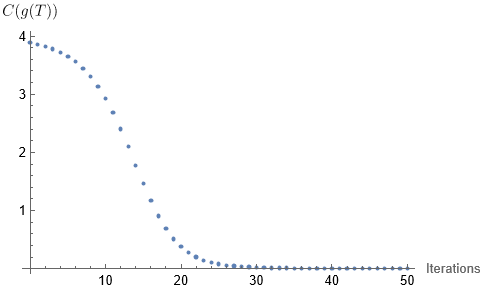
Figure 1. Cost function minimization via line-search algorithm for shooting problem on $SO(3)$

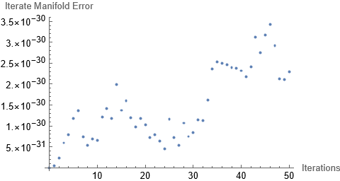
Figure 2. Iterate $SO(3)$ manifold error

This example can be visualized as follows. The objective is to find an element $g_{0}$ of $SO(3)$ such that under the time $T=1$ flow of $F$, $g(1)=g_{\text{target}}$ where $g(0)=g_{0}$. For this example, $g_{\text{target}}$ is chosen to be a $\pi/2$ counterclockwise rotation about the $z$-axis, i.e., in the $xy$ plane. Thus, we can imagine some test mass located at $\vec{v}\in\mathbb{R}^{3}$ which is rotated by $g(t)$, which generates a curve $g(t)\vec{v}$. In particular, choosing $\vec{v}=\hat{x}$, the unit vector in the $x$ direction, then the curve produced from rotating the test mass should end at $g_{\text{target}}\hat{x}=\hat{y}$. Each iteration in the algorithm generates such a curve. In Figure 3, several such curves are shown, with the initial point in the curve $g_{0}\hat{x}$ marked. Additionally, the desired terminal point $g_{\text{target}}\hat{x}$ is marked.

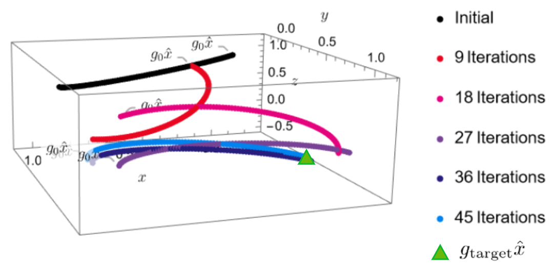
Figure 3. Visualization of the shooting problem on $SO(3)$ using a test mass over several iterations

Parameter Sensitivity Example. For our second example, we consider the following problem of the form (3.10),

$$\min_{u\in U}C( g(T))\equiv\frac{1}{2}\|g(T)-g_{\text{target}}\|_{F}^{2},$$

such that $$\dot{g}(t)=F(g(t),u),\ t\in(0,T),$$

$$g(0)=g_{0}.$$

Thus, this optimal control problem is to find $u\in U$ such that the vector field $F(\cdot,u)$ steers the initial condition $g_{0}\in G$ to some desired terminal-value $g_{\text{target}}\in G$.

We again take $G=SO(3)$. We will assume that $F$ is a parameter-dependent left-invariant vector field $F(g,u)=gX(u)$, where $u\in\mathbb{R}^{3}$ parametrizes $\mathfrak{so}(3)$ as

$$X(u)=\begin{pmatrix}0&-u_{z}&u_{y}\\ u_{z}&0&-u_{x}\\ -u_{y}&u_{x}&0\end{pmatrix}.$$

For simplicity, we take $g_{0}=\text{Id}_{3\times 3}=g_{\text{target}}$ since the analytic answer is known: $F$ should be the zero vector field, since $g_{0}=g_{\text{target}}$ and hence, the optimal value of $u$ is $u=(0,0,0)^{T}$. We take an initial guess of $u=(1,2,-1)^{T}$. We again take $T=1$ with $\Delta t=0.01$, using the same retraction as the previous example. We combine the parameter sensitivity, obtained from Algorithm 2, with a simple vector space line-search algorithm,

$$u\leftarrow u-\gamma\frac{d}{du}C,$$

with a fixed line-search step size $\gamma=0.1$. The cost function $C(g(T))$ over 50 iterations is shown in Figure 4.

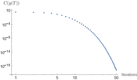
Figure 4. Cost function minimization via line-search algorithm for optimal control problem on $SO(3)$

4. Conclusion and Future Research Directions

In this paper, we developed continuous and discrete global Type II variational principles on the cotangent bundle of a Lie group $G$. In the discrete setting, the Type II variational principle leads to a structure-preserving variational integrator on $T^{*}G$ which we showed to be symplectic and momentum-preserving. Subsequently, we applied these Type II variational principles to the class of adjoint Hamiltonian systems on $T^{*}G$. This results in a structure-preserving method to perform adjoint sensitivity analysis on Lie groups, allowing one to exactly compute sensitivities in optimization problems subject to the dynamics of an ODE on $G$.

One research direction which we are currently pursuing is to explore the geometry of adjoint sensitivity analysis in the infinite-dimensional setting, with the application of PDE-constrained optimization in mind. It would be interesting to synthesize this line of research with the ideas presented in this paper, to develop Hamiltonian integrators for PDEs where the solutions are valued in Lie groups, algebras, or more generally, solutions which are stationary sections over principal and fibre bundles associated to a structure group $G$, such as gauge field theories (see, for example, [39; 19]). It would be particularly interesting to extend the Type II multisymplectic Hamiltonian variational integrators developed in [48] to apply to the setting of Lie groups-valued fields, in order to investigate the role of multisymplectic integrators for adjoint sensitivity analysis in both space and time.

Another natural research direction would be to explore the applications of geometric structure-preserving adjoint sensitivity analysis on Lie groups. One such application is the training of neural networks via backpropagation. In particular, if a neural network is viewed as a discretization of a neural ODE [10], then backpropagation can be viewed as a discretization of the corresponding adjoint equation [38]. As is discussed in [38], utilizing symplectic methods to perform backpropagation leads to efficient methods for training neural networks. It would be interesting to utilize the methods presented in this paper to perform symplectic backpropagation of neural networks where the neural ODE evolves over a Lie group, which would arise in group-equivariant neural networks [11; 24] where a Lie group symmetry is a fundamental feature of the neural network. In particular, the reduction theory for adjoint systems on Lie groups that was developed in this paper would be relevant.

References

• Absil et al. [2008] P.-A. Absil, R. Mahony, and R. Sepulchre. Optimization Algorithms on Matrix Manifolds. Princeton University Press, 2008.
• Barbero-Liñán and Martín de Diego [2021] M. Barbero-Liñán and D. Martín de Diego. Retraction maps: a seed of geometric integrators. ArXiv, abs/2106.00607, 2021.
• Benettin and Giorgilli [1994] G. Benettin and A. Giorgilli. On the Hamiltonian interpolation of near to the identity symplectic mappings with application to symplectic integration algorithms. J. Stat. Phys., 74:1117–1143, 1994.
• Benning et al. [2019] M. Benning, E. Celledoni, M. J. Ehrhardt, B. Owren, and C.-B. Schönlieb. Deep learning as optimal control problems: Models and numerical methods. J. Comput. Dyn., 6(2):171–198, 2019.
• Bobenko and Suris [1999] A. I. Bobenko and Yu. B. Suris. Discrete time Lagrangian mechanics on Lie groups, with an application to the Lagrange top. Commun. Math. Phys., 204:147–188, 1999.
• Bou-Rabee and Marsden [2009] N. Bou-Rabee and J. E. Marsden. Hamilton–Pontryagin integrators on Lie groups part I: Introduction and structure-preserving properties. Found. Comput. Math., 9:197–219, 2009.
• Cacuci [1981] D. G. Cacuci. Sensitivity theory for nonlinear systems. I. Nonlinear functional analysis approach. J. Math. Phys., 22(12):2794–2802, 1981.
• Cao et al. [2003] Y. Cao, S. Li, L. Petzold, and R. Serban. Adjoint sensitivity analysis for differential-algebraic equations: The adjoint DAE system and its numerical solution. SIAM J. Sci. Comput., 24(3):1076–1089 (14 pages), 2003.
• Celledoni and Iserles [2000] Elena Celledoni and Arieh Iserles. Approximating the exponential from a Lie algebra to a Lie group. Math. Comp., 69(232):1457–1480, 2000.
• Chen et al. [2018] R. T. Q. Chen, Y. Rubanova, J. Bettencourt, and D. Duvenaud. Neural ordinary differential equations. In Proceedings of the 32nd International Conference on Neural Information Processing Systems, NIPS’18, page 6572–6583, Red Hook, NY, USA, 2018. Curran Associates Inc.
• Cohen and Welling [2016] T. Cohen and M. Welling. Group equivariant convolutional networks. In M. F. Balcan and K. Q. Weinberger, editors, Proceedings of The 33rd International Conference on Machine Learning, volume 48 of Proceedings of Machine Learning Research, pages 2990–2999, New York, New York, USA, 20–22 Jun 2016. PMLR.
• d’Alembert [1743] J. d’Alembert. Traité de dynamique. 1743.
• Delgado-Téllez and Ibort [2003] M. Delgado-Téllez and A. Ibort. A panorama of geometrical optimal control theory. Extracta mathematicae, 18(2):129–151, 2003.
• Echeverría-Enríquez et al. [2003] A. Echeverría-Enríquez, J. Marín-Solano, M.C. Muñoz-Lecanda, and N. Román-Roy. Geometric reduction in optimal control theory with symmetries. Reports on Mathematical Physics, 52(1):89–113, 2003.
• Fahnestock et al. [2006] E. G. Fahnestock, T. Lee, M. Leok, N. H. McClamroch, and D. J. Scheeres. Polyhedral potential and variational integrator computation of the full two body problem. Proc. AIAA/AAS Astrodynamics Specialist Conf., AIAA-2006-6289, 2006.
• Giles and Pierce [2000] M. B. Giles and N. A. Pierce. An introduction to the adjoint approach to design. Flow, Turbulence and Combustion, 65:393–415, 2000.
• Griewank [2003] A. Griewank. A mathematical view of automatic differentiation. In Acta Numer., volume 12, pages 321–398. Cambridge University Press, 2003.
• Hairer et al. [2006] E. Hairer, C. Lubich, and G. Wanner. Geometric Numerical Integration: Structure-preserving algorithms for ordinary differential equations, volume 31 of Springer Series in Computational Mathematics. Springer-Verlag, Berlin, second edition, 2006.
• Hamilton [2017] M. J. D. Hamilton. Mathematical Gauge Theory. Springer Cham, 2017.
• Ibragimov [2006] N. H. Ibragimov. Integrating factors, adjoint equations and Lagrangians. Journal of Mathematical Analysis and Applications, 318(2):742–757, 2006.
• Ibragimov [2007] N. H. Ibragimov. A new conservation theorem. J. Math. Anal. Appl., 333(1):311–328, 2007.
• Iserles et al. [2000] A. Iserles, H. Munthe-Kaas, S. P. Nørsett, and A. Zanna. Lie-group methods. In Acta Numerica, volume 9, pages 215–365. Cambridge University Press, 2000.
• Kobilarov and Marsden [2011] M. B. Kobilarov and J. E. Marsden. Discrete geometric optimal control on Lie groups. IEEE Transactions on Robotics, 27(4):641–655, 2011.
• Kondor and Trivedi [2018] R. Kondor and S. Trivedi. On the generalization of equivariance and convolution in neural networks to the action of compact groups. In Jennifer Dy and Andreas Krause, editors, Proceedings of the 35th International Conference on Machine Learning, volume 80 of Proceedings of Machine Learning Research, pages 2747–2755. PMLR, 10–15 Jul 2018.
• Lee [2012] J. M. Lee. Introduction to Smooth Manifolds. Springer New York, NY, 2012.
• Lee et al. [2005] T. Lee, N. H. McClamroch, and M. Leok. A Lie group variational integrator for the attitude dynamics of a rigid body with applications to the 3D pendulum. Proc. IEEE Conf. on Control Applications, pages 962–967, 2005.
• Lee et al. [2007a] T. Lee, M. Leok, and N. H. McClamroch. Lie group variational integrators for the full body problem in orbital mechanics. Celestial Mechanics and Dynamical Astronomy, 98(2):121–144, 2007a.
• Lee et al. [2007b] T. Lee, M. Leok, and N. H. McClamroch. Lie group variational integrators for the full body problem. Comput. Methods Appl. Mech. Engrg., 196(29-30):2907–2924, 2007b.
• Lee et al. [2021] T. Lee, T. Tao, and M. Leok. Variational symplectic accelerated optimization on Lie groups. Proc. IEEE Conf. on Decision and Control, pages 233–240, 2021.
• Leok and Ohsawa [2011] M. Leok and T. Ohsawa. Variational and geometric structures of discrete Dirac mechanics. Found. Comput. Math., 11(5):529–562, 2011.
• Leok and Zhang [2011] M. Leok and J. Zhang. Discrete Hamiltonian variational integrators. IMA J. Numer. Anal., 31(4):1497–1532, 2011.
• Li and Petzold [2004] S. Li and L. Petzold. Adjoint sensitivity analysis for time-dependent partial differential equations with adaptive mesh refinement. Journal of Computational Physics, 198(1):310–325, 2004.
• Li and Petzold [2003] S. Li and L. R. Petzold. Solution adapted mesh refinement and sensitivity analysis for parabolic partial differential equation systems. In L. T. Biegler, M. Heinkenschloss, O. Ghattas, and B. van Bloemen Waanders, editors, Large-Scale PDE-Constrained Optimization, pages 117–132. Springer, Berlin, 2003.
• Ma and Rowley [2010] Z. Ma and C. W. Rowley. Lie–Poisson integrators: A Hamiltonian, variational approach. Int. J. Numer. Meth. Engng., 82:1609–1644, 2010.
• Marsden and Ratiu [1999] J. E. Marsden and T. S. Ratiu. Introduction to Mechanics and Symmetry. Springer New York, NY, 1999.
• Marsden and West [2001] J. E. Marsden and M. West. Discrete mechanics and variational integrators. Acta Numer., 10:317–514, 2001.
• Marsden et al. [1999] J. E. Marsden, S. Pekarsky, and S. Shkoller. Discrete Euler–Poincaré and Lie–Poisson equations. Nonlinearity, 12(6):1647, 1999.
• Matsubara et al. [2021] T. Matsubara, Y. Miyatake, and T. Yaguchi. Symplectic adjoint method for exact gradient of neural ODE with minimal memory. In Advances in Neural Information Processing Systems, 2021.
• Nakahara [2003] M. Nakahara. Geometry, Topology, and Physics. CRC Press, second edition, 2003.
• Nguyen et al. [2016] V. T. Nguyen, D. Georges, and G. Besançon. State and parameter estimation in 1-D hyperbolic PDEs based on an adjoint method. Automatica, 67(C):185–191, May 2016. ISSN 0005-1098.
• Pierce and Giles [2000] N. A. Pierce and M. B. Giles. Adjoint recovery of superconvergent functionals from PDE approximations. SIAM Rev., 42(2):247–264, 2000.
• Ross [2005] I. M. Ross. A roadmap for optimal control: The right way to commute. Ann. NY Acad. Sci., 1065(1):210–231, 2005.
• Ross and Fahroo [2001] M. Ross and F. Fahroo. A pseudospectral transformation of the convectors of optimal control systems. IFAC Proc. Ser., 34(13):543–548, 2001.
• Sanz-Serna [2016] J. M. Sanz-Serna. Symplectic Runge–Kutta schemes for adjoint equations, automatic differentiation, optimal control, and more. 58(1):3–33, 2016.
• Schmitt and Leok [2017] J. M. Schmitt and M. Leok. Properties of Hamiltonian variational integrators. IMA Journal of Numerical Analysis, 38(1):377–398, 2017.
• Sirkes and Tziperman [1997] Z. Sirkes and E. Tziperman. Finite difference of adjoint or adjoint of finite difference? Mon. Weather Rev., 125(12):3373–3378, 1997.
• Tang [1994] Y.-F. Tang. Formal energy of a symplectic scheme for Hamiltonian systems and its applications (i). Computers & Mathematics with Applications, 27(7):31 – 39, 1994.
• Tran and Leok [2022a] B. Tran and M. Leok. Multisymplectic Hamiltonian variational integrators. International Journal of Computer Mathematics (Special Issue on Geometric Numerical Integration, Twenty-Five Years Later), 99(1):113–157, 2022a.
• Tran and Leok [2022b] B. Tran and M. Leok. Geometric methods for adjoint systems. (preprint, arxiv/2205.02901 [math.OC]), 2022b.
• Vankerschaver et al. [2012] J. Vankerschaver, H. Yoshimura, and M. Leok. The Hamilton--Pontryagin principle and multi-Dirac structures for classical field theories. J. Math. Phys., 53(7):072903 (25 pages), 2012.
• Wang et al. [2012] Q. Wang, K. Duraisamy, J. J. Alonso, and G. Iaccarino. Risk assessment of scramjet unstart using adjoint-based sampling. AIAA J., 50(3):581--592, 2012.
• Yoshimura and Marsden [2006a] H. Yoshimura and J. E. Marsden. Dirac structures in Lagrangian mechanics Part I: Implicit Lagrangian systems. J. Geom. Phys., 57(1):133--156, 2006a.
• Yoshimura and Marsden [2006b] H. Yoshimura and J. E. Marsden. Dirac structures in Lagrangian mechanics Part II: Variational structures. J. Geom. Phys., 57(1):209--250, 2006b.