Chiral magnetic phases in Moire bilayers of magnetic dipoles

Abstract

In magnetic insulators, the sense of rotation of the magnetization is associated with novel phases of matter and exotic transport phenomena. Aimed to find new sources of chiral magnetism rooted in intrinsic fields and geometry, we study twisted square bilayers of magnetic dipoles with easy plane anisotropy. For no twist, each lattice settles in the antiferromagnetic zig-zag magnetic state and orders antiferromagnetically to the other layer. The moire patterns that result from the mutual rotation of the two square lattices influence such zig-zag order, giving rise to several magnetic phases that depict non-collinear magnetic textures with chiral motifs that break both time and inversion symmetry. For certain moire angles, helical and toroidal magnetic orders arise. These novel phases can be further manipulated by changing the vertical distance between layers. We show that the dipolar interlayer interaction originates an emergent twist-dependent chiral magnetic field orthogonal to the direction of the zig-zag chains, which is responsible for the internal torques conjugated to the toroidal orders.

I Introduction

Chiral magnetic textures are promising building blocks for storing information and offer new venues for the transport of energy in magnetic insulators Casher and Susskind (1974); Tomita et al. (2018); Thiaville and Fert (1992). The onset of such chiral textures is usually conditioned to the presence of antisymmetric spin interactions associated with spin-orbit effects such as the Dzyaloshinskii-Moriya (DM) interaction Dzyaloshinskii (1960, 1958); Heyderman and Stamps (2013); Togawa et al. (2016) or dipolar interactions. Indeed, for lattices of magnetic dipoles featuring out-of-plane anisotropy, the dipolar coupling among all point dipoles gives rise to antisymmetric interactions manifesting in chiral internal magnetic fields Mellado et al. (2023); Paula and Tapia (2023); Yu and Bauer (2021); Ray and Das (2021); Shindou et al. (2013); Lucassen et al. (2019). Among magnetic chiral orders, the study of skyrmions Nagaosa and Tokura (2013); Mohylna et al. (2022); Camosi et al. (2018) has led to a considerable amount of research motivating the inclusion of an elegant mathematical formalism in the field of topological defects, which is suitable to characterize a plethora of helical and chiral structures Schulz et al. (2012); Shaban et al. (2023). While finding materials that realize skyrmionic lattices is an active field of research, finding fields that can efficiently manipulate skyrmions and other topological textures as domain walls is crucial to moving the field to the next stage. More recently, ferrotoroidal phases Dong et al. (2015); Spaldin et al. (2008); Zimmermann et al. (2014); Kuprov et al. (2022) have attracted much interest because of their putative role in the manifestation of the magnetoelectric effect Astrov (1960); Date et al. (1961); Siratori et al. (1992); Ederer and Spaldin (2007); Mellado et al. (2020). Ferrotoroidicity has been defined as a fourth form of ferroic order and consists of a vortex-like magnetic state with zero magnetization and a spontaneously occurring toroidal moment. Because the toroidic order has zero magnetization, the main challenge is finding a conjugate field that couples to the toroidic ferroic order. Recent experiments with permalloy nanoislands interacting via dipolar coupling indeed manifested the ferrotoroidic phase and have achieved local control of the ferrotoroidicity by scanning a magnetic tip, thus widening the possibilities of control on chiral phases Lehmann and Lehmann (2022). In the same direction, the ideas of “twistronics” where the control over electric phases is achieved by the relative rotation between 2D layers of van der Waals materials Klebl et al. (2022); Xiao et al. (2020), which include graphene-based structures Andrei et al. (2021); He et al. (2021), transition-metal dichalcogenides Tran et al. (2019); Xiao et al. (2021), 2D magnets Li and Cheng (2020); Begum Popy et al. (2022), and thin films have motivated a related paradigm of twisted bilayer structures in magnetic systems. This approach does not rely on the engineering of correlated flat bands but can produce interesting new phases by combining known nontrivial properties of constituent monolayers Heyderman and Stamps (2013). While in heterostructures, the spin-wave control is accomplished by tuning the individual layer thicknesses and external fields, in magnetic insulators, the relative twist of bilayers with antiferromagnetic and ferromagnetic spin couplings was predicted to give rise to noncollinear magnetic textures for small twist angles between layers Hejazi et al. (2020); Yang et al. (2023); Li and Cheng (2020); Shimizu et al. (2021); Claassen et al. (2022); Luo et al. (2022). Some of these predictions have been tested recently in experiments Song et al. (2021).

Summary of results: motivated by the search of novel magnetic chiral phases and based on the ideas of twistronics, here we study the dynamics of magnetic dipoles placed at bilayers of square lattices and show that moire arrays of magnetic dipoles give rise to novel chiral magnetic phases absent in the untwisted counterparts. We find that depending on the twist angle $\theta$ and the distance between the layers $h$, the system mutates from an antiferromagnetic zig-zag pattern at zero twists to a set of chiral magnetic configurations which go from periodic arrays of well-defined magnetic antiferromagnetic toroidal patterns to disordered twisted phases passing through helical periodic configurations. Toroidal correlations are easily tuned by varying $\theta$ and $h$. We explain the chiral dipolar orders in terms of a chiral internal magnetic field which arises from the relative twist among the dipolar layers.

The rest of the paper is organized as follows. Section II describes square and moire lattices, the system of dipoles, and the inter and intra-layer dipolar interactions that arise. The different magnetic phases that emerge when the twist angle and the distance between layers is varied are described in sections III and IV. In section V we study the chiral magnetic fields that arise due to the twist and which are responsible for the chiral phases reported in section III. Section VI is devoted to concluding remarks. Appendix A shows details of molecular dynamics simulations used to solve the dynamics of each interacting dipole in the bilayer system, while Appendix B shows details of calculations shown in V.

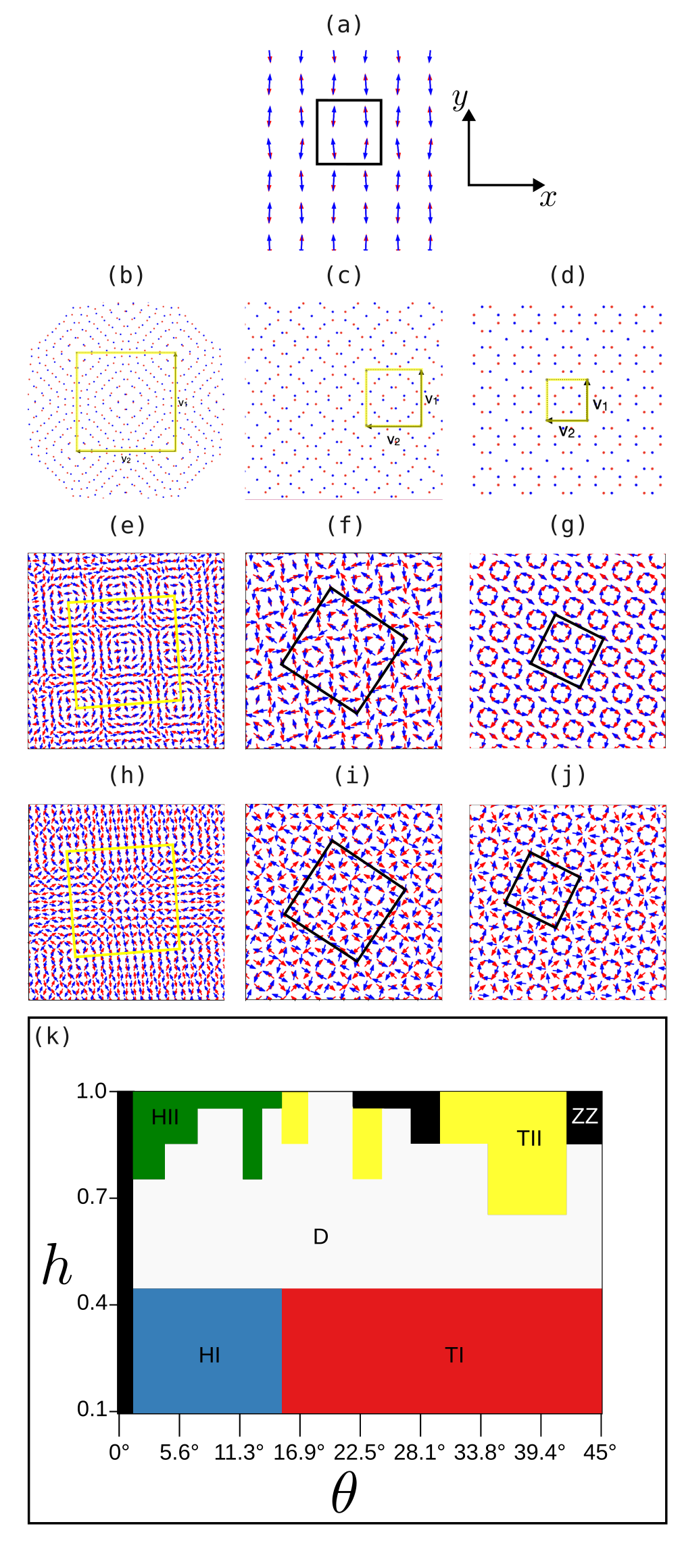
Figure 1: (a) The zig-zag order (ZZ) of the bilayer system for $\theta=0$. (b-d) Moire patterns obtained for twist angles (b) $\theta_{6,7}=8.79^{\circ}$, (c) $\theta_{2,3}=22.61^{\circ}$ and (d) $\theta_{1,2}=36.86^{\circ}$. Black long arrows show the moire lattice primitive vectors $v_{1}$ and $v_{2}$ in each case. (f-j) Real space dipolar configurations obtained from the numerical solution of the equations of motion for systems with (e) $\theta_{2,3}$ and $h=0.1$ featuring phase Helical I (HI), (f) $\theta_{2,3}$ and $h=0.1$ featuring phase Toroidal I (TI), (g) $\theta_{1,2}$ and $h=0.1$ featuring phase TI, (h) $\theta_{6,7}$ and $h=1$ featuring phase Helical II (HII), (i) $\theta_{2,3}$ and $h=1.0$ featuring phase Toroidal II (TII) and (j) $\theta_{1,2}$ and $h=0.9$ featuring phase TII. In all cases small blue arrows illustrate dipoles in layer 1 while red small arrows dipoles in lattice 2. Yellow squares indicate the moire lattice unit cell, while black squares indicate the magnetic unit cell. (k) Phase Diagram in terms of the twist angle $\theta$ and the dimensionless interlayer distance $h$.

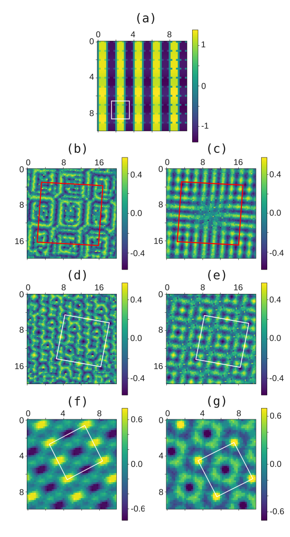
Figure 2: (a) Density plot of the magnetization of a dipolar layer featuring the ZZ order.(b-g) Density plots of the $z$-component of toroidal moment in twisted bilayers featuring phases (b) Helicoidal I: $\theta_{6\,7}=8.78^{\circ}$, $h=0.1$. (c) Helicoidal II: $\theta_{6\,7}=8.78^{\circ}$, $h=1.4$. (d) Toroidal I: $\theta_{2\,3}=22.62^{\circ}$, $h=0.1$. (e) Toroidal II: $\theta_{2\,3}=22.62^{\circ}$, $h=1.4$. (f) Toroidal I: $\theta_{1\,2}=36.87^{\circ}$, $h=0.1$. (g) Toroidal II: $\theta_{1\,2}=36.87^{\circ}$, $h=0.9$.

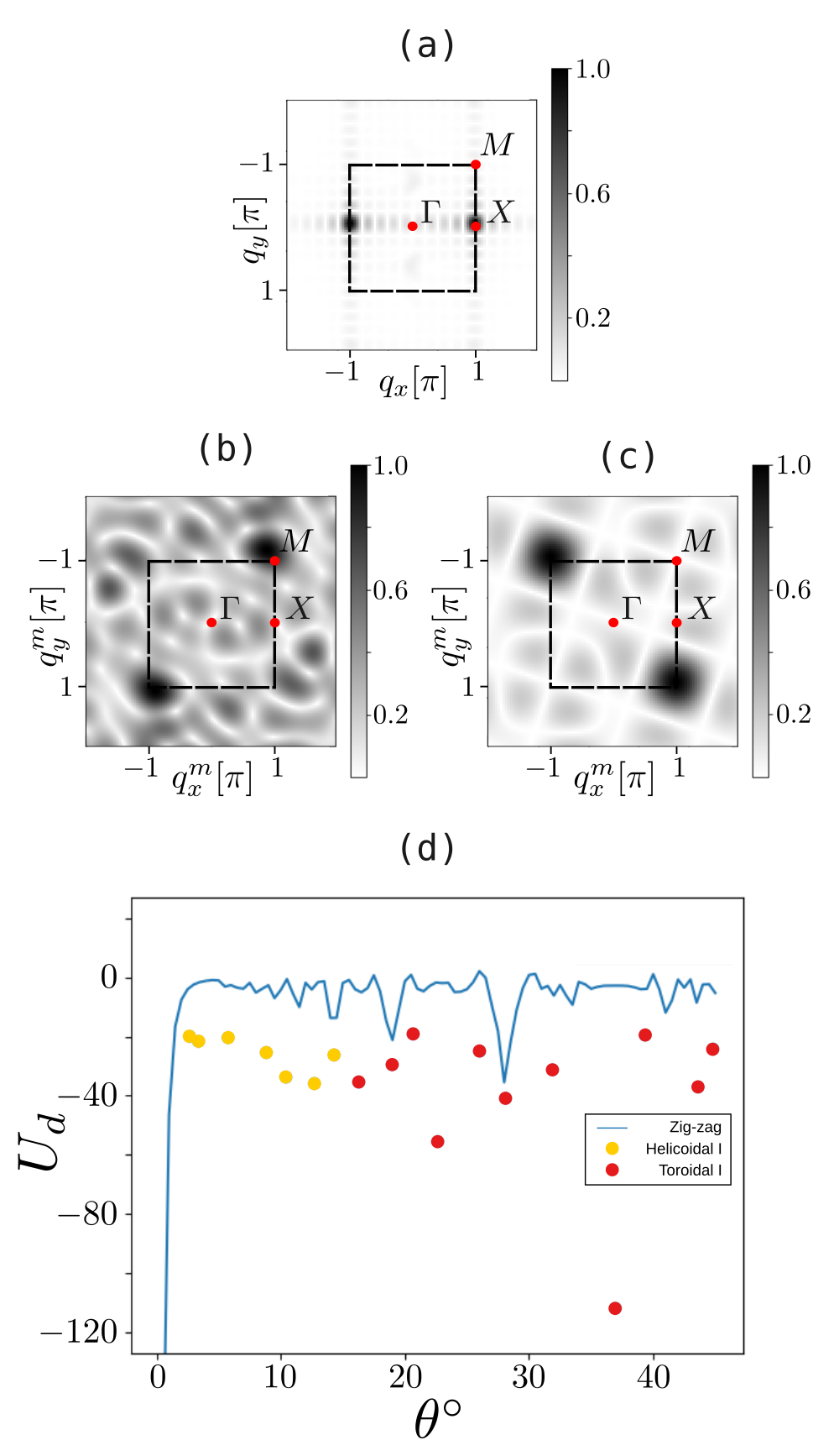
Figure 3: Density plot of the structure factor of the order parameters: (a) the magnetization for a single layer with zig-zag order , and the toroidal moment for Toroidal I phase obtained for (b) ($\theta_{23}=22.61^{\circ}$, $h=0.1$) and (c) ($\theta_{12}=36.87^{\circ}$, $h=0.1$). The dipolar energy obtained for simulations with $h=0.1$ as a function of $\theta$. The solid line shows the dipolar energy of the zig-zag configuration for different angles, while the dots show the energies obtained from the relaxation dynamics. The color of the dots indicates the phase obtained in the simulation: yellow for Helicoidal I and red for Toroidal I.

II Model

The bilayer system consists of two identical square lattices with lattice constant $a$ that extend in the $\hat{x}-\hat{y}$ plane and are stacked at a distance $h$ along the orthogonal $\hat{z}$ direction. At the $n=n_{s}^{2}$ vertices of each square layer of side $L=an_{s}$, $n$ magnetic dipoles are placed. They interact through the full long-range dipolar interaction with all other dipoles of the bilayer system:

$$U_{d}=\frac{g}{2}\sum_{\mu,\nu}^{2}\sum_{i,j}^{n}\frac{\hat{m}_{i}^{\mu}\cdot\hat{m}_{j}^{\nu}-3(\hat{m}_{i}^{\mu}\cdot\hat{r}_{ij}^{\mu,\nu})(\hat{m}_{j}^{\nu}\cdot\hat{r}_{ij}^{\mu,\nu})}{|{\bm{r}}_{i}^{\mu}-{\bm{r}}_{j}^{\nu}|^{3}}$$ (1)

where $\hat{\bm{r}}_{ij}^{\mu\nu}=\frac{({\bm{r}}_{i}^{\mu}-{\bm{r}}_{j}^{\nu})}{|{\bm{r}}_{i}^{\mu}-{\bm{r}}_{j}^{\nu}|}$ denotes the unit vector joining dipole $\hat{\bm{m}}_{i}^{\mu}$ at site $i$ and layer $\mu$ and dipole $\hat{\bm{m}}_{i}^{\nu}$ at site $j$ and layer $\nu$. $g=\frac{u_{0}m_{0}^{2}}{4\pi a^{3}}$ sets an energy scale Mellado et al. (2023) and contains the physical parameters of the system, such as $a$, the lattice constant along $x$ and $y$ directions, $u_{0}$, the magnetic permeability, and $m_{0}$, the intensity of the magnetic moments. Each layer has the full symmetry of the square Bravais lattice. They are set apart along $\hat{z}$ by distance $z=ha$ where $h$ is a positive real number in the range $h\in(0.1,1)$. Dipoles can rotate in the $\hat{x}-\hat{y}$ plane respect to a local axis fixed at their vertices, and have unit vector $\hat{m}_{i}^{\mu}=(m_{i,x}^{\mu},m_{i,y}^{\mu})=(\cos\alpha_{i}^{\mu},\sin\alpha_{i}^{\mu})$ where $\alpha_{i}^{\mu}$ defines the polar rotation angle of dipole i at layer $\mu$. Hereafter the magnetic moments are normalized by $m_{0}$.

Global rotations between layer are performed with respect to axis $\hat{z}$ located at the center of the two layers. The twisted bilayer system forms a crystal only for a discrete set of commensurate rotation angles. We focus on commensurate twist geometries that are amenable to numerical study using the standard Bloch representation. Hence we rotate the layers around specific angles that respond to the equation Kariyado and Vishwanath (2019): $\mathrm{\theta}_{p,q}=2\arctan(p/q)$, where p and q are natural numbers, and the angle is in radians. These types of rotations generate systems called moire geometries, where the patterns depend on $\mathrm{\theta}_{p,q}$ Kariyado and Vishwanath (2019). We note that any commensurate twist can be described by an integer valued ‘twist’ vector $v=(p,q)$ as shown in Figs.1(b-d). The corresponding moire unit cell comprises of $\mathrm{2}(p^{2}+q^{2})$ sites. We rotate the two perfectly aligned square lattices in opposite directions by $\mathrm{\theta}_{p,q}/2$, which leads to the sites originally at the locations $v$ and $\bar{v}=(-p,q)$ to lie atop each other. The unit cells for a selection of commensurate twist angles are illustrated in Fig.1(b-d).

Writing the unit vectors characterizing each layer as ${\bf a}_{1}$ and ${\bf a}_{2}$, the moire pattern induced by twist has a periodicity of ${\bf v}_{1}$ and ${\bf v}_{2}$, which is explicitly written as

$${\bf v}_{i}=v_{i}\hat{z}\times{\bf a}_{i}/(\sin\frac{\theta}{2})$$ (2)

Hermann (2012). The reciprocal lattice vectors of the first Brillouin zone of the moire lattice in each case are given by ${\bf G}_{i}=\frac{2\pi}{{\bf{v}_{i}}}$.

Next we consider the dipolar interaction between all dipoles of the bilayer at zero twist. By separating $\mathrm{U}_{d}$ in intra and inter-layer interactions $U_{d}^{\mu\mu}$ and $U_{d}^{\mu\nu}$, and identifying contributions between pair of dipoles with director vector along the square lattice symmetry axes $\hat{n}_{i}\in(\hat{x},\hat{y})$ and along any other direction, it is easy to see that dipoles prefer to align ferromagnetically with neighbours located along one of the $\hat{n}_{i}$ axes and antiferromagnetically with dipoles along the other orthogonal axis. Given the symmetry of the square lattice, the ground state magnetic configuration is already determined by dipolar interactions at the nearest neighbors level. Without loss of generality the square lattice can be seen as a collection of chains of dipoles along the $\hat{n_{1}}$ direction that extend parallel along the orthogonal direction $\hat{n_{2}}$. We can separate dipoles along the axis $\hat{n_{2}}$ in two sublattices $s_{a}\in(s_{1},s_{2})$ which correspond to the sets of odd and even positions along $\hat{n_{2}}$. Thus regardless the layer, the dipolar energy of the system can be separated in the contribution from dipoles interacting in the same sublattice and dipoles interacting in different sublattices: $U_{d}=\sum_{s_{a}}U_{d}^{(s_{a})}+U_{d}^{(s_{a},s_{b})}$. It is easy to verify that parallel dipoles minimize their energy when they point in opposite senses while collinear dipoles prefer to point in the same sense. If we choose all dipoles to be parallel to $\hat{n_{1}}$, then in units of g the dipolar interaction between dipoles in the same and different sublattices becomes respectively $U_{d}^{(s_{a})}=\sum_{s_{a}}\sum_{i,j\in s_{a}}\frac{\hat{m_{i}}^{s_{a}}\cdot\hat{m_{j}}^{s_{a}}}{(r_{ij})^{3}}(1-3(\frac{(r_{ij}^{n_{1}})^{2}}{(r_{ij})^{2}}))$ and $U_{d}^{(s_{a},s_{b})}=\sum_{s_{a},s_{b}}\sum_{i\in s_{a}j\in s_{b}}\frac{\hat{m_{i}}^{s_{a}}\cdot\hat{m_{j}}^{s_{a}}}{(r_{ij})^{3}}(1-3(\frac{(r_{ij}^{n_{1}})^{2}}{(r_{ij})^{2}}))$. A dipole in $s_{1}$, has two nearest neighbors in $s_{1}$ along $\hat{n}_{1}$ and two in $s_{2}$ along $\hat{n}_{2}$, and at the nearest neighbour level we get $U_{d}^{1nn}=\frac{\hat{m_{i}}^{s_{1}}\cdot\hat{m_{j}}^{s_{1}}}{(1+h^{2})^{3}}(1-\frac{3}{(1+h^{2})^{2}})+\frac{\hat{m_{i}}^{s_{1}}\cdot\hat{m_{j}}^{s_{2}}}{(1+h^{2})^{3}}$. The energy is minimized when dipoles in the same sublattice are ferromagnetic and dipoles in different sublattices are antiferromagnetically arranged. At second nearest neighbours level, interactions happen only between dipoles in different sublattices and though they favour the ferromagnetic interactions between $s_{1}$ and $s_{2}$, these are proportional to $\sim\frac{1}{(2+h^{2})^{3}}$ and therefore are overcomed by the antiferromagnetic first neighbour interaction. Third nearest neighbours interactions occur only between dipoles in the same sublattice and favour a ferromagnetic coupling between dipoles consistent with the first neighbour interaction.

The addition of another layer at zero twist angle further stabilizes the zig-zag order in each layer. The relative orientation of dipoles in the two layers at a distance $h$ is antiferromagnetic, which indeed corresponds to the most favourable magnetic configuration between two parallel magnetic dipoles. Magnetization and staggered magnetization in the bilayer system are defined $\rm{\bf M}=\frac{1}{n}\sum_{i}^{n}{\bf m}_{i}$ and $\rm{\bf N}=\frac{1}{n}\sum_{i}^{n}({\bf m}_{i}^{s_{1}}-{\bf m}_{i}^{s_{2}})$ respectively.

III Phase Diagram

To examine the possible equilibrium magnetic configurations of twisted dipolar bilayers, we solved the equations of motion of each dipole when the lattices are mutually rotated by $\theta/2$ in opposite senses and for a set of interlayer distances $h$, using molecular dynamics simulations. Details are presented in Appendix  A. In the simulations, each dipole $i$ consists of a magnetic bar with inertia moment $I$ and magnetic moment intensity $m_{0}$, which rotates with angle $\alpha_{i}$ respect to its local axis of rotation. The evolution of $\alpha_{i}$ is due to the torques $\mathcal{T}_{i}$ produced by dipolar interaction of dipole $i$ with all other dipoles in the lattice. The angular rotation has damping, product of the friction at the rotation axis as shown by Eq.9.

The twist angle determines the moire pattern of the bilayer while $h$ changes the strength of the interlayer interactions. Indeed, depending on $\theta$ and $h$, dipoles settle into six magnetic phases. Real space dipolar configurations obtained from the molecular dynamics simulations are shown in Fig.1(a) and Fig.1(e-j). At $\theta=0$ and for all the range of $h$ the bilayer settles in a zig-zag antiferromagnetic (ZZ) phase, in the $\hat{x}-\hat{y}$ plane as shown in Fig.1(a). The antiferromagnetic zig-zag phase is a colinear magnetic order along any of the axis $\hat{\bf n}_{1},\hat{\bf n}_{2}\in(\hat{\bf x},\hat{\bf y})$, which doubles the unit cell of the square lattice made of lattice vectors ${\bf a}_{1}=a(1,0)$ and ${\bf a}_{2}=a(0,1)$. As shown in Fig3(a) there are two possible order wave vectors: the two X points at the centers of the edges of the square first Brillouin zone (1BZ), which are half reciprocal vectors ${\bf b}_{1}/2=(\frac{\pi}{a},0)$ and ${\bf b}_{2}/2=(0,\frac{\pi}{a})$. The ZZ phase survives up to $\theta_{21,22}=\sim 2.7$.

Due to the $C_{4}$ symmetry of the square lattice, the maximum twist between layers is reached at $\theta=45^{\circ}$. In this limit the ground state magnetic state depends on the interlayer distance $h$. At $h\in(0.1,0.4)$ dipoles order in a chiral pattern denoted toroidal I (TI). TI is free of M and N and is featured by dipoles arranged in periodic octagonal chiral loops and stars as shown in Figs.1(f) and (g). The orientation of dipoles respect to the center of each loop, determines its vorticity $\mathcal{V}$. The octagonal loops in this phase have a vorticity which follows a zig-zag antiferromagnetic pattern. In the range $h\in(0.5,0.9)$ the periodic dipolar loops disappear and the system settles in a disordered state (D), until at $h=0.9$ it returns to a canted zig-zag pattern with dipoles in both lattices a bit rotated respect to the perfect collinear order of the untwisted bilayer. The previous scenario remains for moire angles in the range $\theta_{p,q}\in(43,45)$.

At angles $\theta_{p,q}\in(39,31)$ a new phase arises for large values of $h$. It is denoted Toroidal II (TII). Similar to TI it features chiral loops but this time their vorticity follows an antiferromagnetic pattern as shown in Fig.1(i) and Fig.1(j). The loops are intercalated by a square arrays of stars which feature zero flux, and by other squared pattern of pairs of dipoles arranged antiferromagnetically.

At moire angles $\theta_{p,q}\in(2,14)$ and for $h\in(0.1,0.4)$, dipoles arrange in phase Helical I (HI) shown in Fig1(e). The magnetic configuration is magnetization free and consists of a square pattern of a squared shaped magnetic vortices that contain several dipoles and resemble in-plane projections of spins in skyrmionic lattices. We describe this phase in more detail in section IV. In this range of $\theta_{p,q}$ and for large h beyond the D phase, the system orders once again and settles in phase Helical II (HII) shown in Fig1(h). HII differs from HI in the size of the magnetic unit cell. Larger interlayer distances are associated with smaller interlayer interactions. In these cases the magnetic unit cell grows, decreasing the order wavevector $q^{ord}$.

IV Antiferromagnetic toroidic orders.

In this section, we focus on helical and toroidal phases. Both break time and inversion symmetries and depict chiral magnetic motifs made out of dipoles of both layers. The main difference is the number of dipoles participating in the pattern that repeats in the magnetic unit cell. Toroidal phases possess periodic clusters that involve eight or fewer dipoles, while the periodic motif in helical phases resembles skyrmion textures in the plane, with many dipoles being part of a sizeable chiral cluster.

In order to characterize toroidal and helical chiral phases, we study their ferrotoroidic order parameter T or toroidization Lehmann and Lehmann (2022), which is derived from the toroidal moment $\bf t=\sum_{i}r_{i}\times m_{i}$, where $r_{i}$ and $m_{i}$ are the position and magnetic moment of the i-th dipole within the unit cell Spaldin et al. (2008). In the toroidal and helical phases, toroidal moments $t_{j}$ belonging to magnetic unit cells $j$ can align in particular ways to form a uniform toroidic state with a spontaneous macroscopic toroidization, ${\bf T}=\sum{\bf t}_{j}$ directed along $\pm\hat{z}$. The sense (sign) of the toroidal moment depends on the handedness of the arrangement of magnetic moments in a magnetic unit cell.

The in-plane helical patterns realized by chiral canted dipoles in these phases can be distinguished in terms of vorticity and helicity, which are used to characterize skyrmion spin structuresNagaosa and Tokura (2013). Introducing the polar coordinates $r=(r\cos\phi,r\sin\phi)$ at the center of each helical motif, for a dipolar texture $m(r)=(\cos\alpha(\phi),\sin\alpha(\phi))$, the vorticity is defined by the integer $\mathcal{V}=[\alpha(\phi)]_{\phi=0}^{\phi=2\pi}/2\pi$ Nagaosa and Tokura (2013). The helicity, $\gamma$ accounts for the phase appearing in $\alpha(\phi)=m\phi+\gamma$ Nagaosa and Tokura (2013). In a toroidal phase with all motifs having the same vorticity, $\gamma$ distinguishes octagonal loops from octagonal stars like those shown in Fig.1(j). Vorticity becomes helpful in distinguishing helical from toroidal phases. While toroidal phases have $\mathcal{V}=1$, helical phases feature dipolar clusters with $\mathcal{V}=-1$.

Figs.2(b-g) show real space density maps of the toroidal order parameter T in moire dipolar bilayers featuring phases TI, TII, HI, and HII, where x and y axes are in units of the square lattice constant. Blue and yellow stripes in the magnetization density plot of Figs.2(a) clearly distinguish ZZ phases. In toroidal phases, the periodic pattern of well-defined yellow and blue dots in Figs.2(d-g) accounts for the antiferromagnetic toroidic order TI and for the antiferromagnetic zig-zag pattern of toroidal loops realized at large $\theta_{1,2}$ and $h\in(0.1,0.4)$. The helical order depicts concentric squared stripes that alternate the sense of T as shown in Figs.2(b-c) .

The wave vector associated with zig-zag and AF orders can be identified in the structure factor of T,

$$S_{q}^{T}=\frac{1}{n}|\sum_{j}T_{j}e^{i{\bf q^{m}}\cdot{\bf r}_{j}}|^{2}$$ (3)

where $q^{m}$ denotes wave vectors in the moire in 1BZ. In Fig.3(a) black dots at the X points of 1BZ are due to the ZZ order in a single lattice.

For twisted bilayers with $\theta_{1,2}$, $\theta_{2,3}$ and for the case of strong interlayer interactions $h=0.1$ the black dots at the M points of 1BZ signal the AF toroidic order in Figs.3(b-c).

In order to show that the magnetic phases of Fig.1 correspond to the ground states of the bilayer systems in the range of $\theta$ and $h$ studied here, in Fig.3(d) the dipolar energy of ZZ phases is compared with that of toroidal and helical phases in the limit of strong interlayer interactions $h=0.1$. For $\theta>0.2$ it is apparent that the ZZ phase becomes too expensive, driving dipoles of both layers to rotate to give way to toroidal and helical phases.

As a hallmark of a ferroic order as the toroidal order, there must be a conjugate field to manipulate the order parameter. For ferrotoroidic materials, this is a toroidal field, a magnetic vortex field violating both space-inversion and time reversal symmetry, as we see next.

V Moire Torques

In the zig-zag equilibrium state at zero twists, the net torques on dipoles of both layers cancel out when they point along any of the $\hat{n}_{i}$ directions. In the previous section, we demonstrated that a relative twist between the layers affects such zig-zag pattern in each lattice and gives rise to canted magnetic configurations whose patterns and motifs can be manipulated by changing either $\theta$ or $h$. In this section, we show that the twist between layers changes the distribution of internal magnetic fields in the system and gives rise to an internal magnetic torque along the $z$ direction, which is responsible for the twisted phases of Fig.1. Consider the origin of the bilayer system $O^{\prime}=(0,0,0)$ at the center of both square lattices. In units of $u_{0}/4\pi$ a dipole ${\bf m}_{i}^{\mu}$ in layer $\mu$ at position ${\bf r}_{i}^{\mu}=(x_{i},y_{i},z_{i})^{\mu}$ respect to $O^{\prime}$ produces a magnetic field

$${\bf B}(r_{i}^{\mu},r_{j}^{\nu})=\frac{3[{\bf m}_{i}^{\mu}\cdot({\bf r}_{i}^{\mu}-{\bf r}_{j}^{\nu})]\cdot({\bf r}_{i}^{\mu}-{\bf r}_{j}^{\nu})-{\bf m}_{i}^{\mu}|{\bf r^{\mu}}_{i}-{\bf r}_{j}^{\nu}|^{2}}{|{\bf r}^{\mu}_{i}-{\bf r}_{j}^{\nu}|^{5}}$$ (4)

at point ${\bf r}_{j}^{\nu}$ in layer $\nu$. An infinitesimal rotation of the coordinate axes through angle $-\theta$ about $\hat{z}$ transforms the components of a magnetic field like those of other vectors such as the coordinates. In addition, $\mathbf{B}(\mathbf{r})$ depends on coordinates $\mathbf{r}$, which must now be expressed in terms of the new ones (see Appendix B for details). The overall infinitesimal change in $\mathbf{B}$, combining the two changes becomes:

$$\delta\mathbf{B}^{\mathrm{twist}}=\bm{\theta}\times\mathbf{B}-\bm{\theta}\cdot(\mathbf{r}\times\nabla)\mathbf{B},$$ (5)

At zero twist, the bilayer system settles in the zig-zag phase. If we take $\pm\hat{y}$ as the direction of the ferromagnetic collinear dipolar chains, we have that the interlayer magnetic field created by a dipole i in layer $\mu$, at points j of lattice $\nu$ is directed along the $\pm\hat{\bm{y}}$ direction (Appendix B). As a consequence, interlayer magnetic field and dipoles are parallel and the total magnetic torque due to interlayer dipolar interactions cancels out $\mathcal{T}(\theta=0)=\sum_{i,j}{\bf m}_{j}^{\nu}\times{\bf B}_{i,(\theta=0)}^{\mu}=0$.

Consider next a finite twist $\theta$. Following Eq.5, the change in ${\bf B}_{i}$ due to $\theta$ is given by:

$$\delta\mathbf{B}_{i}^{\mathrm{twist}}=\theta B_{i,(\theta=0)}(\hat{\bm{z}}\times\hat{\bm{y}})-\theta(\hat{\bm{z}}\cdot(\mathbf{r}\times\nabla))\mathbf{B}_{i},$$ (6)

$$\delta\mathbf{B}_{i}^{\mathrm{twist}}=(\theta B_{i,(\theta=0)},(-x\frac{\partial B_{i,(\theta=0)}}{\partial y}+y\frac{\partial B_{i,(\theta=0)}}{\partial x}),0),$$ (7)

Computing the total interlayer torque due to the twist, once again the $\hat{\bm{y}}$ component of $\delta\mathbf{B}_{i}^{\mathrm{twist}}$ does not produce torque. However the twist originates a magnetic field component along $\hat{\bm{x}}$ which was absent at zero twist. The component orthogonal to the dipolar chains gives rise to a torque along $\hat{\bm{z}}$,

$$\delta\mathcal{T}^{\mathrm{twist}}(h,\theta)=\theta B_{(\theta=0)}(\hat{\bm{z}})$$ (8)

in units of g. Being directed along $\hat{\bm{z}}$, $\delta\mathcal{T}^{\mathrm{twist}}$ rotates dipoles in the $\hat{x}-\hat{y}$ plane and gives rise to the toroidal phases of Fig.1.

VI Conclusion

Dipolar interactions in magnetic insulators with spins larger than one are more frequent than thought a decade ago. Even when their long-range feature contributes to stabilizing magnetic order, it is its anisotropy, the coupling of lattice and magnetic degrees of freedom, which makes it of particular interest for its role in non-collinear spin systems and topological magnetism.

Here, inspired by new research on twisted magnets, we have studied its effect on the magnetic ground states of twisted square bilayers of dipoles. At zero twist, the bilayers settle in a zig-zag antiferromagnetic order, and the interlayer magnetic field has a single component along the zig-zag chains, which gives zero net torque. We found that combining interlayer dipolar interactions between dipoles with an easy plane rotation and an out-of-plane relative rotation between dipolar layers gives rise to a net magnetic torque orthogonal to the bilayer system. The twist torque is due to the emergence of a new interlayer in-plane magnetic field produced by the relative twist between layers. In particular, the component of the twist field directed orthogonal to the zig-zag chains can rotate dipoles from their equilibrium positions, and for certain moire angles, it gives rise to new magnetic orders determined by the underlying moire pattern. The new magnetic phases are magnetization-free and break time and inversion symmetry while depicting chiral motifs that realize a nonzero toroidal moment. Thus, the emergent moire field orthogonal to the zig-zag chains is conjugated to the toroidal moment and, depending on the twist and the interlayer distance (that sets the interlayer coupling), can tune them to order in antiferromagnetic or zig-zag periodic fashions. We expect that our findings will motivate new research on moire versions of other types of dipolar lattices. In particular we anticipate that the study of spin waves in twisted bilayers of dipoles should manifest nontrivial topological effects.

Appendix A Molecular dynamics simulations

We modeled the set of magnetic dipoles as a system of $n$ mechanical rods. The position ${\bf r}_{i}$ ($i=1,\ldots,n$) of the center of mass of dipole $i$ remains fixed during the dynamics, and the orientation $\hat{\bf m}_{i}=(\cos{\alpha_{i}},\sin{\alpha_{i}},0)$ of dipole $i$ is constrained to the $\hat{x}-\hat{y}$ plane due to anisotropy. The magnetic state of the system is specified by the dynamical angular variables $\alpha_{i}$. Magnetic dipoles interact through the full long-range dipolar potential with all other dipoles in the system. The equation of motion of each dynamical angle $\alpha_{i}$ of each inertial dipole reads

$$I\frac{d^{2}\alpha_{i}}{dt^{2}}=\mathcal{T}_{i}^{z}-\xi\frac{d\alpha_{i}}{dt}\,\text{,}$$ (9)

where $I$ denotes the moment of inertia of the magnets and $\xi$ is the damping for the rotation of dipoles respect to their local axis. The first term at the right hand side of equation 9 is the $z$-component of the magnetic torque due to the action of the internal magnetic field from dipolar interaction between all dipoles in the system $\mathcal{T}_{i}^{z}=(\hat{\bf m}_{i}\times\rm{\bf B}_{i})\cdot\hat{\bf z}$, where $\rm{\bf B}_{i}={\partial U_{d}}/{\partial\hat{\bf m}_{i}}$ denotes the internal magnetic field produced by all dipoles but the $i$-$th$ at the position of $\hat{\bf m}_{i}$ and the potential energy defining the dipolar magnetic interactions is given by Eq.1. Following previous experiments Mellado et al. (2023) we used in the simulations dipolar rods with radius $r=0.79\times 10^{-3}$ m, length $L=12.7\times 10^{-3}$ m, and mass $=0.19\times 10^{-4}$ kg, saturation magnetization $M_{s}=1.05\times 10^{6}$ $\rm A/m$, inertial moment $I=1.53\times 10^{-9}$ $\rm kg\,m^{2}$ and magnetic moment $m_{0}=0.026\times 10^{6}$ $\rm A\,m^{2}$. The second term on the RHS of Eq.9 corresponds to a damping term. The viscosity $\xi(\alpha_{i})$ consists of a static and dynamic contributions. Here we used experimental values reported in Mellado et al. (2023). The static part the damping was computed directly by fitting the relaxation of a single rod under a perturbation to the solution $\alpha\sim\exp{-t/\tau_{D}}$. The estimated damping time $\tau_{D}\sim I/\xi$ of a single rod is $\tau_{D}=0.83$ s. The dynamics component is due to the rotation of dipoles in the lattice with other magnets and therefore is dependent on the orientation of the dipole, being maximum when it is orientated perpendicular to $\hat{\bf x}$ axis.
We solved this set of coupled equations using a discretized scheme for the integration of the differential equation, given by the recursion

$$\theta_{i}(t+\Delta t)=f_{a}\theta_{i}(t)-f_{b}\theta_{i}(t-\Delta t)+f_{c}\left(\hat{\bf z}\cdot\mathcal{T}_{i}(t)\right)\,\text{,}$$ (10)

where the functions $f_{a}$, $f_{b}$ and $f_{c}$ corresponds to

$$f_{a}=\frac{2}{1+\Delta t\,\eta(\theta_{i}(t))/2}\,\text{,}$$ (11)

$$f_{b}=\frac{1-\Delta t\,\eta(\theta_{i}(t))/2}{1+\Delta t\,\eta(\theta_{i}(t))/2}\,\text{,}$$ (12)

$$f_{c}=\frac{\Delta t^{2}}{I(1+\Delta t\,\eta(\theta_{i}(t))/2)}\,\text{.}$$ (13)

We initialized the simulations with two square lattices of $n_{s}\times n_{s}$ dipoles and lattice constant $a=2.2\times 10^{-2}\,\rm m$, separated by a distance equal to $h$ (in units of a), and with an offset angle $\theta$ between the lattice vectors of each layer. The dynamical angles $\alpha_{i}$ where initialized in a random configuration. We solved the system of equations Eq.9 numerically during a total time $t=3$ $\rm s$ using an integration step of $\Delta t=4\times 10^{-6}$ $\rm s$. The dynamics are such that the damping term drives the system to a magnetic configuration that locally minimizes the dipolar interactions between magnetic dipoles.

We performed simulations with different interlayer distances $0.1<h<2$ and different moire angles $0^{\circ}<\theta<45^{\circ}$ to characterize the different stationary configurations that appear in the relaxation. We explored system sizes up to $n=50$, and we used a replica method to avoid boundary effects. The simulations were initialized with random magnetic configurations.

The dipolar interactions decay fast with the distance between dipoles $(i,j)$ as $r_{ij}^{-3}$. We implemented a cutoff in the computation of the interactions, equal to $2a$, which shows results consistent with the dynamics observed in simulations with full long-range interactions.

Fig.2 shows a coarse grain of the $z$-component of the toroidal moment T as a function of real space. It can be written at each site as ${\bf T}_{i}={\bf r}_{i}\times{\bf m}_{i}$ and it was calculated using the final magnetic configurations obtained from the simulations. The value of the toroidal moment at position $(x,y)$ was computed numerically by considering a cylinder with center at position $(x,y)$ and a radius of $0.6a$, and then averaging the toroidal moment of the dipoles that are located within the cylinder. We considered cylinders spaced by $a/5$ to create the plots shown in Fig.2.

Appendix B Calculations details

B.1 Interlayer magnetic field in the ZZ phase

The magnetic field produced by a dipole i pointing along the $\hat{y}$ axis and located at layer $\mu$ and sublattice $s_{1}$ in all points j of layer $\nu$ can be separated into inter and intra-sublattice contributions:

$${\bf B}_{i}^{s_{1}}=\frac{(6mn,2m^{2}-4n^{2}-h^{2},3mh)}{(4n^{2}+m^{2}+h^{2})^{\frac{5}{2}}}$$

$${\bf B}_{i}^{s_{2}}=\frac{(-3m(2n+1),-2m^{2}+(2n+1)^{2}+h^{2},-3mh)}{((2n+1)^{2}+m^{2}+h^{2})^{\frac{5}{2}}}$$

in units of $g/m_{0}$ and where $n=(\Delta r_{ij}^{x})$, $m=(\Delta r_{ij}^{y})$. After summation over all the j points of layer $\nu$, the x and z components of $B_{i}$ cancel out to give only a non zero coponent along the y direction,

$${\bf B}_{i}=\sum_{m}\big{[}\sum_{n\in s_{1}}\frac{(0,2m^{2}-n^{2}-h^{2},0)}{(n^{2}+m^{2}+h^{2})^{\frac{5}{2}}}$$ (14)

$$+\sum_{n^{\prime}\in s_{2}}\frac{(0,-2m^{2}+n^{\prime 2}+h^{2},0)}{(n^{\prime 2}+m^{2}+h^{2})^{\frac{5}{2}}}\big{]}$$

B.2 Effect of rotation of coordinates on a Magnetic field

An infinitesimal rotation of the coordinate axes through angle $-\theta$ about $\hat{z}$ transforms the coordinates $(x,y,z)\mapsto(x^{\prime},y^{\prime},z^{\prime})$ as follows Weyl (1929):

$$x^{\prime}=x-y\theta,\quad y^{\prime}=y+x\theta,\quad z^{\prime}=z.$$

For a rotation about a general axis $\hat{\mathbf{n}}$ through infinitesimal angle $\theta$,

$$\mathbf{r}^{\prime}=\mathbf{r}+\bm{\theta}\times\mathbf{r},$$ (15)

where $\bm{\theta}=\theta\hat{\mathbf{n}}$. The inverse transform expresses the old coordinates in terms of the new ones:

$$\mathbf{r}=\mathbf{r}^{\prime}-\bm{\theta}\times\mathbf{r}^{\prime}.$$

The magnetic field changes as a result of the rotation in two ways. First, it is a vector quantity, so its components change like those of other vectors such as the coordinate (15):

$$\mathbf{B}^{\prime}=\mathbf{B}+\bm{\theta}\times\mathbf{B}.$$ (16)

Second, $\mathbf{B}(\mathbf{r})$ depends on coordinates $\mathbf{r}$, which must now be expressed in terms of the new ones $\mathbf{r}^{\prime}$:

$$\mathbf{B}^{\prime}(\mathbf{r}^{\prime}) = \mathbf{B}(\mathbf{r})=\mathbf{B}(\mathbf{r}^{\prime}-\bm{\theta}\times\mathbf{r}^{\prime})$$

$$= \mathbf{B}(\mathbf{r}^{\prime})-[(\bm{\theta}\times\mathbf{r}^{\prime})\cdot\nabla^{\prime}]\mathbf{B}(\mathbf{r}^{\prime}).$$

The overall infinitesimal change in $\mathbf{B}$, combining the two changes (16) and (B.2), can be written in a compact form:

$$\delta\mathbf{B}^{\mathrm{twist}}=\bm{\theta}\times\mathbf{B}-\bm{\theta}\cdot(\mathbf{r}\times\nabla)\mathbf{B}.$$ (18)

where we have dropped the primes.

References

- Casher and Susskind (1974) A. Casher and L. Susskind, Physical Review D 9, 436 (1974).
- Tomita et al. (2018) S. Tomita, H. Kurosawa, T. Ueda, and K. Sawada, Journal of Physics D: Applied Physics 51, 083001 (2018).
- Thiaville and Fert (1992) A. Thiaville and A. Fert, Journal of magnetism and magnetic materials 113, 161 (1992).
- Dzyaloshinskii (1960) I. E. Dzyaloshinskii, Soviet Physics JETP 10, 628 (1960).
- Dzyaloshinskii (1958) I. Dzyaloshinskii, J. Phys. Chem. Solids 4, 241 (1958).
- Heyderman and Stamps (2013) L. J. Heyderman and R. L. Stamps, Journal of Physics: Condensed Matter 25, 363201 (2013).
- Togawa et al. (2016) Y. Togawa, Y. Kousaka, K. Inoue, and J.-i. Kishine, Journal of the Physical Society of Japan 85, 112001 (2016).
- Mellado et al. (2023) P. Mellado, A. Concha, K. Hofhuis, and I. Tapia, Scientific reports 13, 1245 (2023).
- Paula and Tapia (2023) M. Paula and I. Tapia, Journal of Physics: Condensed Matter 35, 164002 (2023).
- Yu and Bauer (2021) T. Yu and G. E. Bauer, Chirality, Magnetism and Magnetoelectricity: Separate Phenomena and Joint Effects in Metamaterial Structures pp. 1–23 (2021).
- Ray and Das (2021) S. Ray and T. Das, Physical Review B 104, 014410 (2021).
- Shindou et al. (2013) R. Shindou, J.-i. Ohe, R. Matsumoto, S. Murakami, and E. Saitoh, Physical Review B 87, 174402 (2013).
- Lucassen et al. (2019) J. Lucassen, M. J. Meijer, O. Kurnosikov, H. J. Swagten, B. Koopmans, R. Lavrijsen, F. Kloodt-Twesten, R. Frömter, and R. A. Duine, Physical review letters 123, 157201 (2019).
- Nagaosa and Tokura (2013) N. Nagaosa and Y. Tokura, Nature nanotechnology 8, 899 (2013).
- Mohylna et al. (2022) M. Mohylna, F. G. Albarracín, M. Žukovič, and H. Rosales, Physical Review B 106, 224406 (2022).
- Camosi et al. (2018) L. Camosi, N. Rougemaille, O. Fruchart, J. Vogel, and S. Rohart, Physical Review B 97, 134404 (2018).
- Schulz et al. (2012) T. Schulz, R. Ritz, A. Bauer, M. Halder, M. Wagner, C. Franz, C. Pfleiderer, K. Everschor, M. Garst, and A. Rosch, Nature Physics 8, 301 (2012).
- Shaban et al. (2023) P. Shaban, I. Lobanov, V. Uzdin, and I. Iorsh, arXiv preprint arXiv:2304.08306 (2023).
- Dong et al. (2015) S. Dong, J.-M. Liu, S.-W. Cheong, and Z. Ren, Advances in Physics 64, 519 (2015).
- Spaldin et al. (2008) N. A. Spaldin, M. Fiebig, and M. Mostovoy, Journal of Physics: Condensed Matter 20, 434203 (2008).
- Zimmermann et al. (2014) A. S. Zimmermann, D. Meier, and M. Fiebig, Nature communications 5, 4796 (2014).
- Kuprov et al. (2022) I. Kuprov, D. Wilkowski, and N. Zheludev, Science Advances 8, eabq6751 (2022).
- Astrov (1960) D. N. Astrov, J. Exptl. Theoret. Phys. (U.S.S.R.) 38, 984 (1960).
- Date et al. (1961) M. Date, J. Kanamori, and M. Tachiki, Journal of the Physical Society of Japan 16, 2589 (1961).
- Siratori et al. (1992) K. Siratori, K. Kohn, and E. Kita, Acta Phys. Pol. A 81, 431 (1992).
- Ederer and Spaldin (2007) C. Ederer and N. A. Spaldin, Physical Review B 76, 214404 (2007).
- Mellado et al. (2020) P. Mellado, A. Concha, and S. Rica, Physical Review Letters 125, 237602 (2020).
- Lehmann and Lehmann (2022) J. Lehmann and J. Lehmann, Toroidal Order in Magnetic Metamaterials pp. 113–131 (2022).
- Klebl et al. (2022) L. Klebl, Q. Xu, A. Fischer, L. Xian, M. Claassen, A. Rubio, and D. M. Kennes, Electronic Structure 4, 014004 (2022).
- Xiao et al. (2020) Y. Xiao, J. Liu, and L. Fu, Matter 3, 1142 (2020).
- Andrei et al. (2021) E. Y. Andrei, D. K. Efetov, P. Jarillo-Herrero, A. H. MacDonald, K. F. Mak, T. Senthil, E. Tutuc, A. Yazdani, and A. F. Young, Nature Reviews Materials 6, 201 (2021).
- He et al. (2021) F. He, Y. Zhou, Z. Ye, S.-H. Cho, J. Jeong, X. Meng, and Y. Wang, ACS nano 15, 5944 (2021).
- Tran et al. (2019) K. Tran, G. Moody, F. Wu, X. Lu, J. Choi, K. Kim, A. Rai, D. A. Sanchez, J. Quan, A. Singh, et al., Nature 567, 71 (2019).
- Xiao et al. (2021) F. Xiao, K. Chen, and Q. Tong, Physical Review Research 3, 013027 (2021).
- Li and Cheng (2020) Y.-H. Li and R. Cheng, Physical Review B 102, 094404 (2020).
- Begum Popy et al. (2022) R. Begum Popy, J. Frank, and R. L. Stamps, Journal of Applied Physics 132 (2022).
- Hejazi et al. (2020) K. Hejazi, Z.-X. Luo, and L. Balents, Proceedings of the National Academy of Sciences 117, 10721 (2020).
- Yang et al. (2023) B. Yang, Y. Li, H. Xiang, H. Lin, and B. Huang, Nature Computational Science 3, 314 (2023).
- Shimizu et al. (2021) K. Shimizu, S. Okumura, Y. Kato, and Y. Motome, Physical Review B 103, 184421 (2021).
- Claassen et al. (2022) M. Claassen, L. Xian, D. M. Kennes, and A. Rubio, Nature communications 13, 4915 (2022).
- Luo et al. (2022) Z.-X. Luo, U. F. Seifert, and L. Balents, Physical Review B 106, 144437 (2022).
- Song et al. (2021) T. Song, Q.-C. Sun, E. Anderson, C. Wang, J. Qian, T. Taniguchi, K. Watanabe, M. A. McGuire, R. Stöhr, D. Xiao, et al., Science 374, 1140 (2021).
- Kariyado and Vishwanath (2019) T. Kariyado and A. Vishwanath, Physical Review Research 1, 033076 (2019).
- Hermann (2012) K. Hermann, Journal of Physics: Condensed Matter 24, 314210 (2012).
- Weyl (1929) H. Weyl, Bulletin of the American Mathematical Society 35, 716 (1929).