Convergence from discrete to continuous non-linear Fourier transform

Abstract.

In this note we study the convergence of discrete to continuous non-linear Fourier transforms. Relations between spectral problems and questions for complex function theory provide a new approach for the study of scattering problems and non-linear Fourier transform [Pol23]. In particular, non-linear Fourier transform can be viewed from the perspective of spectral problems. Results in [MP23, PZ23] can be viewed as results for non-linear Fourier transform. These results are similar to some convergence problems for discrete non-linear Fourier transform considered in [Tao02] and [TT12].

1. Introduction

We study the convergence from discrete to continuous inverse non-linear Fourier transform in this note.

Over the past few decades, a wealth of evidence has indicated that scattering problems for differential operators can be seen as a non-linear version of the classical Fourier transform [Tao02, TT12].

Naturally, one can ask whether certain properties of the linear Fourier transform hold in the non-linear scattering setting. These problems have been studied over the past several decades and remain active today. Most of developments and details of these problems can be found in [Sil17] and references therein. One of the more recent developments in non-linear Fourier transform is pointwise convergence.

Pointwise convergence of Fourier transform on ${\mathbb{R}}$, due to L. Carleson [Car66], is one of the fundamental results in Fourier analysis. Poltoratski recently proved a non-linear analog of the Carleson theorem on the half-line ${\mathbb{R}}_{+}$ [Pol23]. His approach is based on the study of resonances of Dirac systems using spectral theory for differential operators and complex function theory, which is independent of the existing results. Although it had been known that scattering and spectral problems are closely related to non-linear Fourier transform, this connection was never made explicit until [Pol23].

The non-linear Fourier transform defined in [TT12] relies on a limit, similar to its linear counterpart. Moreover, the definition is only ”explicit” for sequences. In general, there is not a formula like the linear Fourier transform for the non-linear transform. In section 5, we propose an alternative definition for the non-linear Fourier transform, which relies on the spectral measure of the underlying Dirac (or canonical) system. With this definition, there is a natural way to construction a sequence whose non-linear Fourier transform converge to the transform of a continuous function. Similar problems were considered in [TT12] without much detail. We are able to provide some of the details for this approach using our modified definition.

The explicit formula for discrete non-linear Fourier transform in [Tao02] involves a product of matrix exponential, which is hard to compute. Even for a finite sequence, it is challenging to obtain an explicit example from the formula. However, this formula for sequences is the only example for non-linear Fourier transform in the literature as far as we know. Our modified definition uses the spectral measure of a Dirac system and avoids explicitly taking the limit. With this definition, we are able to connect some sequences with their non-linear Fourier transforms, and obtain some examples for discrete non-linear Fourier transform.

The main object in [TT12] is discrete non-linear Fourier transform. It was mentioned there (without a proof) that NLFTs of discrete sequences can be used to approximate NLFTs of functions. For a Dirac system with pointmasses as ”potentials”, the smaller the distance between adjacent pointmasses is, the larger the period of its spectral measure gets. With the periodization approach used in [PZ23], we are able to construct sequences whose non-linear Fourier transforms converge to the non-linear Fourier transform of a function in the continuous sense.

The paper is organized as follows. We will introduce real Dirac systems and canonical systems in section 2, the basics of Krein-de Branges theory in section 3, and spectral measures in section 4. The definitions of non-linear Fourier transform of locally integrable functions and sequences, as well as some of their properties are contained in section 5. Our main result, using non-linear Fourier transforms of discrete sequences to approximate continuous ones, is in section 7. Finally in section 8 we will provide several explicit examples of the non-linear Fourier transform, which are hard to find in the existing literature.

2. Real Dirac Systems and Canonical Systems

Dirac systems on the right half-line $\mathbb{R}_{+}$ are systems of the form

$$\Omega\dot{X}(t)=zX(t)-Q(t)X(t),\ \ t\in(0,\infty),$$ (1)

where $z\in\mathbb{C}$ is a spectral parameter, $\Omega=\begin{pmatrix}0&1\\ -1&0\end{pmatrix}$ is the symplectic matrix, and $Q(t)=\begin{pmatrix}0&f(t)\\ f(t)&0\end{pmatrix}$ is the potential matrix, where $f(t)$ is a real-valued locally summable function, and $X(t,z)=\begin{pmatrix}u(t,z)\\ v(t,z)\end{pmatrix}$ is the unknown vector-function.

Dirac systems can be rewritten as canonical systems, which form a broad class of second-order differential systems. Canonical systems are $2\times 2$ differential equation systems of the form

$$\Omega\dot{X}(t)=zH(t)X(t),\ \ t\in(t_{-},t_{+}),\ \ -\infty<t_{-}<t_{+}\leqslant\infty,$$ (2)

where $z\in{\mathbb{C}}$ is a spectral parameter, $\Omega=\begin{pmatrix}0&1\\ -1&0\end{pmatrix}$ is the symplectic matrix as before, $H(t)=\begin{pmatrix}h_{11}(t)&h_{12}(t)\\ h_{21}(t)&h_{22}(t)\end{pmatrix}$ is a given matrix-valued function called the Hamiltonian of the system, and $X(t,z)=\begin{pmatrix}u(t,z)\\ v(t,z)\end{pmatrix}$ is the unknown vector-function. Here $H(t)\in\mathbb{R}^{2\times 2}$, $H(t)\in L^{1}_{loc}(\mathbb{R})$, and $H(t)\geqslant 0$ almost everywhere.

For reader’s convenience, we provide details on rewriting real Dirac systems as canonical systems. Details of this process can be found for instance in [MPS].

Let $V$ be the real $2\times 2$ matrix satisfying

$$\begin{cases}\Omega\dot{V}(t)=Q(t)V(t)\\ V(0)=I\end{cases}.$$

The solution is

$$V(t)=\begin{pmatrix}\exp(\int_{0}^{t}f(x)dx)&0\\ 0&\exp(-\int_{0}^{t}f(x)dx)\end{pmatrix}.$$

We claim that this matrix $V(t)$ satisfies $V^{\ast}(t)\Omega V(t)=\Omega$. First note that $V^{\ast}(t_{-})\Omega V(t_{-})=I$. It remains to show that $V^{\ast}(t)\Omega V(t)$ stays constant. We differentiate $V^{\ast}(t)\Omega V(t)$ and obtain

$$\begin{split}\dot{V^{\ast}}(t)\Omega V(t)+V^{\ast}(t)\Omega\dot{V}(t)&=-\left(\Omega\dot{V}(t)\right)^{\ast}V(t)+V^{\ast}(t)\left(-Q(t)V(t)\right)\\ &=\left(Q(t)V(t)\right)^{\ast}V(t)-V^{\ast}(t)Q(t)V(t)=0\end{split}$$

Finally, with a change of variable $X(t)=V(t)Y(t)$, where $X(t)$ is the vector solution in (1), we get

$$\begin{split}&\Omega\dot{\left(V(t)Y(t)\right)}=zV(t)Y(t)-Q(t)V(t)Y(t),\\ &\Omega\dot{V}(t)Y(t)+\Omega V(t)\dot{Y}(t)=zV(t)Y(t)-Q(t)V(t)Y(t),\\ &\cancel{\left(-Q(t)V(t)\right)Y(t)}+\Omega V(t)\dot{Y}(t)=zV(t)Y(t)\cancel{-Q(t)V(t)Y(t)},\\ &V^{\ast}\Omega V(t)\dot{Y}(t)=zV^{\ast}(t)V(t)Y(t),\end{split}$$

which is a canonical system with Hamiltonian

$$H^{D}=V^{\ast}(t)V(t)=\begin{pmatrix}\exp\left(2\int_{0}^{t}f(x)dx\right)&0\\ 0&\exp\left(-2\int_{0}^{t}f(x)dx\right)\end{pmatrix}.$$

If distributions are allowed in $f$, all canonical systems with diagonal and determinant-normalized Hamiltonians can be brought to real Dirac form as well. Therefore, we also allow a combination of real pointmasses to be in the potential of Dirac systems. In other words, we broaden the class of functions $f$ we allow in (1) where all $f$ satisfying $\exp(2\int_{0}^{t}f(x)dx)\in L^{1}_{loc}$ can be the potential of a Dirac system. Krein-de Branges theory for canonical systems applies to Dirac systems, see [deB68, Dym70, Rem18, Rom14]. The next section is a brief summary of the theory that we will need in this note.

3. Krein-de Branges theory

3.1. Inner function and Clark measure

This brief discussion on inner function and Clark measure is primarily based on [Pol15] and [PS06].

An inner function is a function in $H^{\infty}({\mathbb{C}_{+}})$ with absolute boundary value $1$ almost everywhere on ${\mathbb{R}}$, here $H^{\infty}({\mathbb{C}_{+}})$ denotes the space of bounded analytic functions on ${\mathbb{C}_{+}}$.

Analytic functions with non-negative imaginary parts are called Herglotz functions.

Theorem 3.1 (Herglotz representation theorem for ${\mathbb{C}_{+}}$).

Let $m\mathrel{\mathop{\mathchar 58\relax}}{\mathbb{C}_{+}}\to{\mathbb{C}_{+}}$ be analytic. Then there exists a finite positive measure $\mu$ on ${\mathbb{R}}$ and constant $A\geqslant 0$ such that

$$m(z)=\Re{m(i)}+Az+\frac{1}{\pi}\int\left(\frac{1}{t-z}-\frac{t}{1+t^{2}}\right)d\mu(t).$$ (3)

For every inner function $\Theta(z)$, by the Cayley transform there is a corresponding Herglotz function

$$m(z)=i\frac{1+\Theta(z)}{1-\Theta(z)}.$$

Given a Herglotz function $m(z)$, the corresponding $\Theta$ is inner if and only if the measure $\mu$ in (3) is singular with respect to the Lebesgue measure. Since we will use this to define the Clark measure, we write it down explicitly

$$\Re\frac{1+\Theta(z)}{1-\Theta(z)}=Ay+\frac{1}{\pi}\int\frac{yd\mu(t)}{(x-t)^{2}+y^{2}},$$ (4)

where $A$ can be interpreted as a point mass at infinity, the measure $\mu$ is singular to the Lebesgue measure, Poisson finite ($\int\frac{d\mathinner{\!\left\lvert\mu(t)\right\rvert}}{1+t^{2}}<\infty$), and supported on the set on ${\mathbb{R}}$ where the non-tangential limits of $\Theta(z)$ are $1$. The measure $\sigma=\mu+A\delta_{\infty}$ is called the Clark measure of $\Theta$.

For a given inner function $\Theta(z)$, we can define a family of Clark measures. The measure we just obtained is usually denoted by $\sigma_{1}$. Let $\alpha$ be a unimodular number, then $\tilde{\Theta}(z)=\bar{\alpha}\Theta(z)$ is still an inner function and we can obtain a different Clark measure $\tilde{\sigma}$ from (4). This Clark measure is usually denoted by $\sigma_{\alpha}$. We call the family of measures $\{\sigma_{\alpha}\}_{\mathinner{\!\left\lvert\alpha\right\rvert}=1}$ the family of Clark measures of an inner function $\Theta$.

In the case where the inner function $\Theta$ is meromorphic (MIF), we can write down the Clark measure $\sigma$ explicitly

$$\sigma=\sigma_{1}=\frac{2\pi}{\Theta^{\prime}(x)}\delta_{x},\quad\text{where~{}}x\in\{\Theta=1\}.$$

3.2. Model space

For each inner function $\Theta$, we can consider the associated model space

$$K_{\Theta}=H^{2}({\mathbb{C}_{+}})\ominus\Theta H^{2}({\mathbb{C}_{+}}),$$

where $\Theta H^{2}({\mathbb{C}_{+}})=\left\{\Theta(z)f(z)|f(z)\in H^{2}({\mathbb{C}_{+}})\right\}$. Here $\ominus$ is the orthogonal difference between the two sets.

$K_{\Theta}$ is a reproducing kernel Hilbert space. The reproducing kernel is

$$k_{\Theta}(z,w)=\frac{1}{2\pi i}\cdot\frac{1-\Theta(z)\overline{\Theta(w)}}{\overline{w}-z},$$

and for every $f\in K_{\Theta}$, $f(z)=\langle f,k_{\Theta}\rangle_{w}$.

Recall that $\sigma$ is the Clark measure corresponding to the inner function $\Theta$. Functions in $K_{\Theta}$ have non-tangential boundary values $\sigma-$almost everywhere, and can be recovered from the boundary values using the following formula

$$f(z)=\frac{1}{2\pi i}\left(1-\Theta(z)\right)\int f(t)\overline{\left(1-\Theta(t)\right)}dt+\frac{1-\Theta(z)}{2\pi i}\int\frac{f(t)}{t-z}d\sigma(t).$$ (5)

3.3. Entire functions and de Branges spaces

An entire function $E(z)$ is called a Hermite-Biehler function if $|E(z)|>|E(\overline{z})|$ for $z\in\mathbb{C}_{+}$. Given an entire function $E(z)$ of Hermite-Biehler class, define the de Branges’ space $B(E)$ based on $E$ as

$$B(E)=\left\{F\text{~{}entire}\ |\ F/E,F^{\#}/E\in H^{2}(\mathbb{C_{+}})\right\},$$

where $F^{\#}(z)=\overline{F(\overline{z})}$. The space $B(E)$ becomes a Hilbert space when endowed with the scalar product inherited from $H^{2}({\mathbb{C}}_{+})$:

$$[F,G]=\int_{-\infty}^{\infty}F(t)\overline{G(t)}\frac{dt}{|E(t)^{2}|}.$$

We call an entire function real if it is real-valued on ${\mathbb{R}}$. Associated with $E$ are two real entire functions $A=\frac{1}{2}(E+E^{\#})$ and $C=\frac{i}{2}(E-E^{\#})$ such that $E=A-iC$. De Branges’ spaces are also reproducing kernel Hilbert spaces. The reproducing kernels

$$K_{\lambda}(z)=\frac{\overline{E(\lambda)}E(z)-\overline{E^{\#}(\lambda)}E^{\#}(z)}{2\pi i(\overline{\lambda}-z)}=\frac{\overline{C(\lambda)}A(z)-\overline{A(\lambda)}C(z)}{\pi(\overline{\lambda}-z)}$$

are functions from $B(E)$ such that and $[F,K_{\lambda}]=F(\lambda)$ for all $F\in B(E)$, $\lambda\in\mathbb{C}$.

De Branges’ spaces have an alternative axiomatic definition, which is useful in many applications.

Theorem 3.2 ([deB68]).

Suppose that $H$ is a Hilbert space of entire functions that satisfies

• $F\in H$, $F(\lambda)=0$ $\Rightarrow$ $F(z)\frac{z-\overline{\lambda}}{z-\lambda}\in H$ with the same norm,

• $\forall\lambda\notin\mathbb{R}$, the point evaluation is a bounded linear functional on $H$,

• $F\to F^{\#}$ is an isometry.

Then $H=B(E)$ for some entire function $E$ of Hermite-Biehler class.

Every Hermite-Biehler entire function $E(z)$ gives rise to a meromorphic inner function $\Theta(z)=E^{\#}(z)/E(z)$, and a corresponding model space $K_{\Theta}$. There exists an isomorphism between $K_{\Theta}$ and $B(E)$ given by $F\mapsto EF$.

The most elementary example of de Branges spaces is the Paley-Wiener spaces. We denote by $PW_{t}$ the standard Paley-Wiener space: the subspace of $L^{2}({\mathbb{R}})$ consisting of entire functions of exponential type at most $t$. $PW_{t}=B(E)$ with $E(z)=e^{-itz}$. The reproducing kernels of $PW_{t}$ are the sinc functions,

$$\frac{\sin(t(z-\lambda))}{\pi(z-\lambda)}.$$

4. Spectral Measures

4.1. Spectral measure

A solution to (1) is a $C^{2}-$function

$$X(t,z)=X(t,z)=\begin{pmatrix}u(t,z)\\ v(t,z)\end{pmatrix}$$

on $(t_{-},t_{+})$ satisfying the equation. An initial value problem (IVP) for (1) is given by an initial condition $X(t_{-})=c$, $c\in\mathbb{R}^{2}$. Differential equation theory guarantees that every IVP for (1) has a unique solution $X(t,z)$ on $(t_{-},t_{+})$, see for instance chapter 1 of [Rem18].

Let $X(t,z)=\begin{pmatrix}u(t,z)\\ v(t,z)\end{pmatrix}$ be the unique solution for (1) on $(0,t_{+})$ satisfying a self-adjoint initial condition $X(t_{-})=x$, $x\in\mathbb{R}^{2}$. De Branges first observed that the function $E(t,z)=u(t,z)-iv(t,z)$ is an Hermite-Biehler entire function for every fixed $t$.

Every Dirac system delivers a family of nested de Branges’ spaces $B(E(t,z))$: if $t_{-}\leqslant t_{1}<t_{2}\leqslant t_{+}$, then $B(E(t_{1},z))\subseteq B(E(t_{2},z))$, and all such inclusions are isometric.

A positive measure $\mu$ on ${\mathbb{R}}$ is called the spectral measure of (1) corresponding to a fixed self-adjoint boundary condition at $t_{-}$ if all de Branges’ spaces $B(E_{t})$, $t\in[t_{-},t_{+})$ are isometrically embedded into $L^{2}(\mu)$. A spectral measure always exists, and it is unique if and only if

$$\int_{t_{-}}^{t_{+}}\text{trace~{}}H(t)dt=\infty.$$

The case when the integral above is infinite (and the spectral measure is unique) is called the limit point case, otherwise it is called the limit circle case.

Under our assumption for Dirac systems, any spectral measure $\mu$ is Poisson-finite, see for instance [deB68, Rem18].

We will pay special attention to systems whose spectral measures are sampling for all Paley-Wiener spaces $PW_{t}$.

Definition 4.1.

A positive Poisson-finite measure $\mu$ is sampling for the Paley-Wiener space $PW_{t}$ if there exist constants $0<c<C$ such that for all $f\in PW_{t}$

$$c\|f\|_{PW_{t}}\leqslant\|f\|_{L^{2}(\mu)}\leqslant C\|f\|_{PW_{t}}.$$

A positive measure $\mu$ is a Paley-Wiener measure ($\mu\in PW$) if it is sampling for $PW_{t}$ for all $t>0$.

It is not difficult to show that any PW-measure is Poisson-finite. For this and other basic properties of PW-measures, see [MP23] and references therein. We call a canonical system a PW-system if the corresponding de Branges’ spaces $B(E_{t})$ are equal to $PW_{t}$ as sets for all $t$. In this case any spectral measure $\mu$ of the system is a PW-measure. It follows that PW-systems can be equivalently defined as those systems whose spectral measures belong to the PW-class.

Real Dirac systems with locally summable potentials, as a particular case of canonical systems with determinant normalized Hamiltonians, always give rise to PW-spectral measures. For real Dirac systems with pointmasses as the potential, the corresponding spectral measures are periodic.

The class of PW-measures admits the following elementary description.

Definition 4.2.

Let $\mu$ be a positive measure on ${\mathbb{R}}$. We call an interval $I\subseteq\mathbb{R}$ a $(\mu,\delta)$-interval if

$$\mu(I)>\delta,\quad\text{and}\quad\mathinner{\!\left\lvert I\right\rvert}>\delta,$$

where $\mathinner{\!\left\lvert I\right\rvert}$ stands for the length of the interval $I$.

Theorem 4.3.

[MP23] A positive Poisson-finite measure $\mu$ is a Paley-Wiener measure if and only if

• $\sup_{x\in\mathbb{R}}(x,x+1)<\infty$,

• For any $d>0$, there exists $\delta>0$ such that for all sufficiently large intervals $I$, there exist at least $d\mathinner{\!\left\lvert I\right\rvert}$ disjoint $(\mu,\delta)$-intervals intersecting $I$.

We say that a measure $\mu$ has locally infinite support if $\text{supp\ }\mu\cap[-C,C]$ is an infinite set for some $C>0$, or equivalently if $\text{supp\ }\mu$ has a finite accumulation point. For a periodic measure one can easily deduce the following.

Corollary 4.4.

[MP23] A positive locally finite periodic measure is a Paley-Wiener measure if and only if it has locally infinite support.

We will see in section 6 that if pointmasses are allowed to be in the potential $f$ of a Dirac system and the pointmasses are evenly spaced, the corresponding system always gives rise to an even spectral measure.

4.2. Hilbert transform

This section is primarily based on section 19 of [MPS], and this is one of the key ingredient for our alternative definition for the non-linear Fourier transform in section 5.

Denote by $M(t,z)=\begin{pmatrix}A(t,z)&B(t,z)\\ C(t,z)&D(t,z)\end{pmatrix}$ the solution to the matrix initial value problem on the half-line

$$\Omega\dot{M}(t)=zM(t)-Q(t)M(t),\quad M(0)=I,$$ (6)

and $M_{0\to b}(t,z)=\begin{pmatrix}A_{0\to b}(t,z)&B_{0\to b}(t,z)\\ C_{0\to b}(t,z)&D_{0\to b}(t,z)\end{pmatrix}$ the solution to the matrix initial value problem on the interval $(0,b)$

$$\Omega\dot{M}_{0\to b}(t)=zM_{0\to b}(t)-Q(t)M_{0\to b}(t),\quad M(0)=I.$$ (7)

The matrix $M_{0\to b}(t,z)$ is entire with respect to $z$. The first column corresponds to the Neumann boundary condition at $t=0$, and the second column corresponds to the Dirichlet boundary condition at $t=0$.

Definition 4.5.

A matrix $\begin{pmatrix}A(z)&B(z)\\ C(z)&D(z)\end{pmatrix}$ is called a Nevanlinna matrix if all elements are entire functions and the following conditions are satisfied:

• this identity holds:

  $$A(z)D(z)-B(z)C(z)=1;$$

• for any fixed real $t$, the function

  $$w(z)=\frac{A(z)t-B(z)}{C(z)t-D(z)}$$

  satisfies the inequality

  $$\frac{\Im{w(z)}}{\Im{z}}>0.$$

The matrix solutions to the initial value problems 6 and 7 are both Nevanlinna matrices. In the rest of this section, we focus on (7), the case on an interval $(0,b)$. For convenience, we will use $A$ instead of $A_{0\to b}$, and similarly for $B$, $C$ and $D$.

We consider the following objects:

1. $E(z)=A(z)-iC(z)$ is the first Hermite-Biehler entire function, and $\mu_{A}$ is its spectral measure supported on $Z(A)$, $\mu_{C}$ is its spectral measure supported on $Z(C)$. Here $Z(A)$ and $Z(C)$ stand for the zero sets of functions $A(z)$ and $C(z)$ on ${\mathbb{R}}$.

2. $F(z)=A(z)+iB(z)$ is our second Hermite-Biehler entire function. We consider the associated inner function

   $$\Theta(z)=\frac{A(z)-iB(z)}{A(z)+iB(z)},$$

   and denote its Clark measures $\sigma_{\alpha}$. Then $\sigma_{-1}$ is supported on $Z(A)$, and $\sigma_{1}$ is supported on $Z(B)$.

Let $\mu^{F}$ be the spectral measure of $F(z)$ on $Z(A)$. Recall from the previous section that

$$\mu_{A}=-\frac{\pi\delta_{x}}{A^{\prime}C},\quad\quad\mu^{F}=\frac{\pi\delta_{x}}{A^{\prime}B},\quad\quad x\in Z(A).$$

On $Z(A)$, since the matrix $M$ is normalized by its determinant, we have $B(z)C(z)=-1$ on $Z(A)$, which is $B(z)=-1/C(z)$. Also note that on $Z(A)$, $\mathinner{\!\left\lvert E\right\rvert}^{2}=\mathinner{\!\left\lvert C\right\rvert}^{2}$ and $\mathinner{\!\left\lvert F\right\rvert}^{2}=\mathinner{\!\left\lvert B\right\rvert}^{2}$. Therefore,

$$\mu_{A}=-\frac{\pi\delta_{x}}{A^{\prime}}\frac{1}{C}=\frac{\pi\delta_{x}}{A^{\prime}}B=\mathinner{\!\left\lvert B\right\rvert}^{2}\frac{\pi\delta_{x}}{A^{\prime}B}=F^{2}\mu_{F}=\sigma_{-1}.$$

Since an inner function can be recovered from its spectral measure via the Schwarz transform, we get that for every finite $t\in(0,b)$,

$$\frac{B(z)}{A(z)}=-\frac{i}{\mathcal{S}_{\sigma_{-1}}}=-\frac{i}{\mathcal{S}_{\mu_{A}}}.$$ (8)

Similarly, we can look at the Hermite-Biehler functions $\tilde{E}(z)=B(z)-iD(z)$ and $\tilde{F}(z)=C(z)+iD(z)$, do a similar calculation and obtain

$$\frac{D(z)}{C(z)}=-\frac{i}{\mathcal{S}_{\tilde{\sigma}_{-1}}}=-\frac{i}{\mathcal{S}_{\mu_{C}}},$$ (9)

where $\tilde{\sigma}$ is the Clark measure of the inner function

$$\tilde{\Theta}(z)=\frac{C(z)-iD(z)}{C(z)+iD(z)}.$$

Equations (8) and (9) play an important role in the alternative definition for the non-linear Fourier transform next chapter.

5. Non-linear Fourier Transform

For reader’s convenience, we provide details on the connection between Hermit-Biehler entire functions and non-linear Fourier transform discussed in [Pol23]. Denote by $E(t,z)$ and $\tilde{E}(t,z)$ the Hermite-Biehler functions corresponding to the Neumann $X(0,z)=\begin{pmatrix}1\\ 0\end{pmatrix}$ and Dirichlet $X(0,z)=\begin{pmatrix}0\\ 1\end{pmatrix}$ boundary conditions, respectively. Then (1) for $E$ and $\tilde{E}$ becomes

$$\frac{\partial}{\partial t}E(t,z)=\left(-zv(t,z)+f(t)u(t,z)\right)-i\left(zu(t,z)-f(t)v(t,z)\right),$$

which yields

$$\frac{\partial}{\partial t}E(t,z)=-izE(t,z)+f(t)E^{\#}(t,z),$$ (10)

with initial conditions $E(0,z)=1-0i=1$ for $E$, and $\tilde{E}(0,z)=0-i=-i$ for $\tilde{E}$.

For each $t\geqslant 0$, define the following entire functions

$$\begin{split}a(t,z)&=\frac{\exp(itz)}{2}\left(E(t,z)+i\tilde{E}(t,z)\right),\\ b(t,z)&=\frac{\exp(itz)}{2}\left(E(t,z)-i\tilde{E}(t,z)\right).\end{split}$$ (11)

As in [Pol23], this notation is slightly different than the one in [Tao02] and [TT12], where their $a$ is $a^{\#}$ here.

The limit of $\left(a(t,z),b(t,z)\right)$ as $t\to\infty$ can be viewed as a non-linear analog of the Fourier transform, if the limit exists in some sense. We denote the limit by $\left(a(\infty,z),b(\infty,z)\right)$. This definition was used for instance in [Tao02]. It is known that when $f\in L^{2}$, the pair $\left(a(t,z),b(t,z)\right)$ converges normally on the half-plane ${\mathbb{C}_{+}}$ (see [Den06]), and the function $b(t,z)/a(t,z)$ converges pointwise on the half-line ${\mathbb{R}}_{+}$ (see [Pol23]).

Using (10), one can show that the matrix

$$G(t,z)=\begin{pmatrix}a^{\#}(t,z)&b^{\#}(t,z)\\ b(t,z)&a(t,z)\end{pmatrix}$$

satisfies the differential equation

$$\frac{\partial}{\partial t}G(t,z)=\begin{pmatrix}0&e^{-2izt}f(t)\\ e^{2izt}f(t)&0\end{pmatrix}G(t,z),$$ (12)

with initial condition $G(0,z)=I$.

Consider a matrix differential equation in the form of (12) with initial condition $G(0,z)=I$. The matrix solution will be of the form

$$G(t,z)=\begin{pmatrix}a^{\#}(t,z)&b^{\#}(t,z)\\ b(t,z)&a(t,z)\end{pmatrix}.$$

The limit of the solution $\left(a(t,z),b(t,z)\right)$ as $t\to\infty$ is analogous to the linear Fourier transform if the limit exists in some sense. This is the definition used in for instance [MTT02].

As in [Pol23], we will pay special attention to the functions

$$\overset{\ \curlywedge}{f}(z)=\frac{b(\infty,z)}{a(\infty,z)},$$

and

$$\overset{\ \curlywedge}{f}_{t}(z)=\frac{b(t,z)}{a(t,z)}.$$

The $\overset{\ \curlywedge}{f}_{t}$’s contain enough information to recover $(a(t,z),b(t,z))$: $a(t,z)$ can be uniquely recovered since $a(t,z)$ is outer for all $t$, positive at $0$, and $a(t,z)$ has absolute value

$$|a(t,z)|=\frac{1}{\sqrt{1-|\overset{\ \curlywedge}{f}_{t}|^{2}}}\quad\text{ on }\mathbb{R},$$

and $b(t,z)=a(t,z)\overset{\ \curlywedge}{f}_{t}$. Under the assumption $f\in L^{2}$, we have $\overset{\ \curlywedge}{f}_{t}\to\overset{\ \curlywedge}{f}$ almost everywhere [Pol23].

This function $\overset{\ \curlywedge}{f}$ also has a nice connection with the spectral measure of the underlying Dirac system: by (11), for every finite $t$, we have

$$\frac{b(t,z)}{a(t,z)}=\frac{E(t,z)-i\tilde{E}(t,z)}{E(t,z)+i\tilde{E}(t,z)}=\frac{1-i\frac{\tilde{E}(t,z)}{E(t,z)}}{1+i\frac{\tilde{E}(t,z)}{E(t,z)}}.$$

Since all the de Branges spaces are isometrically embedded into $L^{2}(\mu)$, both $\mu_{A}$ and $\mu_{C}$ go to $\mu$ as $t\to\infty$. Together with (8), we get

$$\frac{\tilde{u}(t,z)}{u(t,z)},\frac{\tilde{v}(t,z)}{v(t,z)}\to-i\frac{1}{\mathcal{S}_{\mu}(z)},\quad\text{as}\;t\to\infty,$$

where $\mathcal{S}_{\mu}(z)$ is the Schwarz transform

$$\mathcal{S}_{\mu}(z)=\frac{1}{\pi i}\int_{\mathbb{R}}\frac{1}{t-z}-\frac{t}{1+t^{2}}d\mu(t).$$

Then we have

$$\frac{b(t,z)}{a(t,z)}=\frac{1-i\frac{\tilde{E}(t,z)}{E(t,z)}}{1+i\frac{\tilde{E}(t,z)}{E(t,z)}}\to\frac{\mathcal{S}_{\mu}-1}{\mathcal{S}_{\mu}+1}.$$

Based on this, we propose the following definition for the non-linear Fourier transform.

Definition 5.1.

Let $f$ be a real-valued locally summable function on the half-line $\mathbb{R}_{+}$, and $\mu$ be a spectral measure of the real Dirac system with potential $Q=\begin{pmatrix}0&f(x)\\ f(x)&0\end{pmatrix}$. The non-linear Fourier transform (NLFT) of $f$ is

$$\overset{\ \curlywedge}{f}(z)=\frac{\mathcal{S}_{\mu}-1}{\mathcal{S}_{\mu}+1},$$

where $\mathcal{S}_{\mu}(z)$ is the Schwarz transform.

One advantage of this definition is that it avoids taking the limit of $\left(a(t,z),b(t,z)\right)$, which might not exist. The definition above agrees with $\lim_{t\to\infty}\left(a(t,z),b(t,z)\right)$ if such limit exists in some sense. This definition also applies to the discrete case studied by Tao and Thiele in [TT12] since distributions are allowed in the potential $f$. We will discuss the discrete case more in the second half of this section.

This transform $f\to\overset{\ \curlywedge}{f}$ has several properties similar to the linear Fourier transform. The following properties are summarized in [Sil17]:

• Modulation/ frequency shifting: if $h(t)=e^{2ist}{f}(t)$, then $\overset{\ \curlywedge}{h}(z)=\overset{\ \curlywedge}{f}(z-s)$ ;

• Translation / time shifting: if $h(t)=f(t-t_{0})$, then $\overset{\ \curlywedge}{h}(z)=e^{2it_{0}z}\overset{\ \curlywedge}{f}(z)$;

• Time scaling: for $a>0$ and $h(t)=af(at)$, then $\overset{\ \curlywedge}{h}(z)=\overset{\ \curlywedge}{f}(\frac{z}{a})$;

• Linearization at the origin is the Fourier transform :

  $$\overset{\ \curlywedge}{\epsilon f}(z)=\epsilon\hat{f}(z)+\mathcal{O}(\epsilon^{2});$$

• Non-linear Riemann-Lebesgue:

  $$|\overset{\ \curlywedge}{f}(z)|\leqslant\tanh\left(\mathinner{\!\left\lVert f\right\rVert}_{L^{1}(\mathbb{R})}\right);$$

• Non-linear Parseval:

  $$\|f\|_{L^{2}(\mathbb{R})}^{2}=\frac{1}{2}\mathinner{\!\left\lVert\log\left(1-|\overset{\ \curlywedge}{f}|^{2}\right)\right\rVert}_{L^{1}(\mathbb{R})}.$$

Tao and Thiele primarily studied non-linear Fourier transform of discrete sequences in [TT12]. Let $f$ be a combination of evenly spaced pointmasses

$$f(t)=\sum_{n=1}^{\infty}c_{n}\delta_{n}(t).$$

Define $a(N,z)$ and $b(N,z)$ as follows:

$$\begin{split}a(0,z)&=1,\quad b(0,z)=0,\\ \begin{pmatrix}a^{\#}(N,z)&b^{\#}(N,z)\\ b(N,z)&a(N,z)\end{pmatrix}&=\exp\begin{pmatrix}0&c_{N}\exp(-2izN)\\ c_{N}\exp(2izN)&0\end{pmatrix}\begin{pmatrix}a^{\#}(N-1,z)&b^{\#}(N-1,z)\\ b(N-1,z)&a(N-1,z)\end{pmatrix}.\end{split}$$

Note that this is different from the discrete transform in [TT12], since they work with $c_{n}\in\mathbb{T}$. This recursion above can be viewed as a discrete version of (12). In [TT12], the NLFT of $f$ or $\{c_{n}\}$ is defined as the limit of $(a(N,z),b(N,z))$ as $N\to\infty$, if the limit exists in some sense. If $f$ is a finite collection of pointmasses, $\sum_{n=1}^{N}c_{n}\delta_{n}$, then

$$\begin{pmatrix}a^{\#}(\infty,z)&b^{\#}(\infty,z)\\ b(\infty,z)&a(\infty,z)\end{pmatrix}=\prod_{n=1}^{N}\exp\begin{pmatrix}0&c_{n}\exp(-2izn)\\ c_{n}\exp(2izn)&0\end{pmatrix}.$$

Even in the finite product case above, this formula is still only symbolic. However, this is the only NLFT example (we know of) that exists in the literature.

For an infinite one-sided sequence, it is known that the limit of $\left(a(n,z),b(n,z)\right)$ exists when $\{c_{n}\}\in\ell^{p}$, $1\leqslant p\leqslant 2$, see [TT12]. Let $f$ be the potential of the Dirac system, and $\mu$ be the spectral measure, we can use definition 5.1 for the discrete case. The function $\overset{\ \curlywedge}{f}=b(\infty,z)/a(\infty,z)$ satisfies

$$\overset{\ \curlywedge}{f}=\frac{b(\infty,z)}{a(\infty,z)}=\frac{\mathcal{S}_{\mu}-1}{\mathcal{S}_{\mu}+1}.$$

With this connection between discrete NLFT and spectral measures, we will provide one way of explicitly obtaining inverse discrete NLFT in section 7.

6. Inverse Spectral Problems

The goal of inverse spectral problem is to recover the original differential equation from its spectral data. This section summarizes some recent developments on inverse spectral problems for canonical systems.

If $a_{n}$ and $b_{n}$ are trigonometric moments of a given locally finite $2\pi$-periodic measure $\mu$,

$$a_{0}=\frac{\mu([-\pi,\pi])}{2\pi},\ \ a_{n}=\frac{1}{\pi}\int_{-\pi}^{\pi}\cos(nx)\ d\mu(x),\ \ b_{n}=\frac{1}{\pi}\int_{-\pi}^{\pi}\sin(nx)\ d\mu(x),\ n=1,2,...$$

we will formally write $\mu=\sum_{n=0}^{\infty}(a_{n}cos(nx)+b_{n}\sin(nx))$.

The Dirac systems we are using to study the non-linear Fourier transform always give rise to a diagonal determinant normalized canonical systems without jump intervals. Moreover, canonical systems with diagonal Hamiltonians always give rise to even spectral measures (see [MP23] and references therein for details). The following 2 results provide an explicit way of recovering the Hamiltonian matrix in (2) if the spectral measure is even and periodic. Since we only consider systems with even spectral measures, we have $b_{n}=0$ for all $n$.

Theorem 6.1 ([MP23]).

Let $\mu$ be a spectral measure of a system (2). Suppose that $\mu$ is an even $2\pi$-periodic PW-measure, $d\mu(x)=\sum_{n=0}^{\infty}a_{n}cos(nx)dx$.

Consider the infinite Toeplitz matrix

$$J=\begin{pmatrix}a_{0}&\frac{a_{1}}{2}&\frac{a_{2}}{2}&\frac{a_{3}}{2}&\ldots\\ \frac{a_{1}}{2}&a_{0}&\frac{a_{1}}{2}&\frac{a_{2}}{2}&\ldots\\ \frac{a_{2}}{2}&\frac{a_{1}}{2}&a_{0}&\frac{a_{1}}{2}&\ldots\\ \frac{a_{3}}{2}&\frac{a_{2}}{2}&\frac{a_{1}}{2}&a_{0}&\ldots\\ \vdots&\vdots&\vdots&\vdots&\ddots\\ \end{pmatrix}.$$

Denote by $J_{n}$ the $(n+1)\times(n+1)$ sub-matrix on the upper-left corner of $J$. Then $h_{11}(t)$ in the Hamiltonian is a step function with

$$h_{11}(t)=\Sigma(J_{n}^{-1})-\Sigma(J_{n-1}^{-1})\;\text{on}\;\Big{(}\frac{n}{2},\frac{n+1}{2}\Big{]},\ n=0,1,2,\ldots$$

where $\Sigma$ denotes the sum of all elements in the matrix, and $J_{-1}^{-1}=0$.

Via a change of variable one can extend the last statement to $2T-$periodic measures:

Corollary 6.2.

[PZ23] Let $\mu$ be an even $2T$-periodic PW-measure, $d\mu(x)=\left(\sum_{n=0}^{\infty}a_{n}cos\left(\frac{2n\pi}{2T}x\right)\right)dx$. Consider the infinite Toeplitz matrix

$$J=\begin{pmatrix}a_{0}&\frac{a_{1}}{2}&\frac{a_{2}}{2}&\frac{a_{3}}{2}&\ldots\\ \frac{a_{1}}{2}&a_{0}&\frac{a_{1}}{2}&\frac{a_{2}}{2}&\ldots\\ \frac{a_{2}}{2}&\frac{a_{1}}{2}&a_{0}&\frac{a_{1}}{2}&\ldots\\ \frac{a_{3}}{2}&\frac{a_{2}}{2}&\frac{a_{1}}{2}&a_{0}&\ldots\\ \vdots&\vdots&\vdots&\vdots&\ddots\\ \end{pmatrix}.$$

Denote by $J_{n}$ the $(n+1)\times(n+1)$ sub-matrix on the upper-left corner of $J$. Then $h_{11}(t)$ in the Hamiltonian is a step function with

$$h_{11}(t)=\Sigma(J_{n}^{-1})-\Sigma(J_{n-1}^{-1})\;\text{on}\;\Big{(}\frac{n\pi}{2T},\frac{(n+1)\pi}{2T}\Big{]},n=0,1,2,\ldots$$

where $\Sigma$ denotes the sum of all elements in the matrix, and $J_{-1}^{-1}=0$.

Theorem 6.1 also connects inverse spectral problems with orthogonal polynomials on the unit circle (OPUC).

Theorem 6.3 ([MP23]).

The value of the $n$-th step of $h_{11}(t)$ is $\mathinner{\!\left\lvert\varphi_{n}(1)\right\rvert}^{2}$, where $\varphi_{n}(z)$ is the $n$-th orthonormal polynomial on $\mathbb{T}$ with $\mu_{\mathbb{T}}=\frac{1}{2\pi}\mu|_{[-\pi,\pi]}$.

For non-periodic spectral measures, the inverse spectral problem can be solved using a ”periodization” approach. Let $\mu$ be an even spectral measure of a canonical system. We denote by $\mu_{T}$ its $2T-$periodization, defined as $\mu_{T}(S)=\mu(S)$ for $S\subseteq[-T,T]$, and and extended periodically to the rest of $\mathbb{R}$.

Theorem 6.4.

[PZ23] Let $\mu$ be an even spectral measure of a PW-system, and $\mu_{T}$ be its periodizations, then $h_{11}^{T}\overset{\ast}{\to}h_{11}$ as $T\to\infty$.

Here, $h_{11}^{T}\overset{\ast}{\to}h_{11}$ means $\int_{0}^{\infty}h_{11}^{T}(t)\phi(t)dt{\to}\int_{0}^{\infty}h_{11}(t)\phi(t)dt$ as $T\to\infty$, for every continuous compactly supported function $\phi$ on $\mathbb{R}_{+}$.

7. Main Results

If a family evenly spaced pointmasses is the potential of a Dirac system, the corresponding canonical system has a diagonal Hamiltonian and $h_{11}$ is a step function of step size $1/2$, which is the case considered in theorems 6.1 and 6.3. Via direct computation, theorem 6.3 yields the following result:

Theorem 7.1.

Let $\mu$ be an even $2\pi-$periodic PW-measure, and let $\{\varphi_{n}\}_{n=0}^{\infty}$ be the family of polynomials orthonormal in $L^{2}_{\frac{\mu}{2\pi}}(\mathbb{T})$. The inverse non-linear Fourier transform of $\frac{S_{\mu}-1}{S_{\mu}+1}$ is

$$\sum_{n=1}^{\infty}\log\left(\frac{|\varphi_{n}(1)|}{|\varphi_{n-1}(1)|}\right)\delta_{n/2}.$$

Let $w(x)$ be the absolutely continuous part of the measure $\mu$. The spectral measures we consider in this note are known satisfy the Szegö condition: $\log\mathinner{\!\left\lvert w(x)\right\rvert}\in L^{1}(\Pi)$, see [Den06] for details on this and related results. If an even PW-measure satisfies the Szegö condition, we can take it to be the spectral measure of real Dirac system, take its inverse non-linear Fourier transform, and obtain a discrete sequence of point masses. It can be shown that this sequence has to be square summable, which is the following corollary, see [TTT] for details.

Corollary 7.2.

Let $\mu$ be an even PW-measure on the unit circle $\mathbb{T}$ satisfying the Szegö condition, and let $\{\varphi_{n}\}_{n=0}^{\infty}$ be the family of polynomials orthonormal in $L^{2}_{\frac{\mu}{2\pi}}(\mathbb{T})$. The sequence

$$\log\left(\frac{|\varphi_{n}(1)|}{|\varphi_{n-1}(1)|}\right)$$

is in $\ell_{2}$.

It was mentioned in [TT12] that NLFT of sequences can be used to approximate NLFT of functions and obtain a convergence result for inverse NLFT. Our next goal is to use this idea to get a convergence result on inverse NLFT.

Let $\mu$ be the spectral measure of the Dirac system, and $\mu_{T}$ be the $2T-$periodization of $\mu$, defined by $\mu_{T}(S)=\mu(S)$ if $S\subseteq[-T,T]$ and $\mu_{T}$ is $2T-$periodic. Denote by $h_{11}^{T}$ the first entry in the Hamiltonian corresponding to $\mu_{T}$,

$$\begin{split}\overset{\ \curlyvee}{f^{T}}(t)&=\frac{1}{2}\frac{d}{dt}\log\left(h_{11}^{T}(t)\right),\\ \overset{\ \curlyvee}{f}(t)&=\frac{1}{2}\frac{d}{dt}\log\left(h_{11}(t)\right),\end{split}$$

and $f^{T}$ and $f$ the non-linear Fourier transforms of $\overset{\ \curlyvee}{f^{T}}$ and $\overset{\ \curlyvee}{f}$ respectively.

Functions from the closed unit ball in $H^{\infty}({\mathbb{C}_{+}})$ (or $H^{\infty}({\mathbb{D}})$) are called Schur functions. Based on definition 5.1, NLFTs of one-sided sequences $\{a_{n}\}_{n>0}\in\ell^{p}$ and functions $f\in L^{p}$ are Schur functions.

Theorem 7.3.

Let $f(z)$ be a Schur function corresponding to the spectral measure $\mu$ of a Dirac system. Recall that

$$f(z)=\frac{\mathcal{S}_{\mu}(z)-1}{\mathcal{S}_{\mu}(z)+1}.$$

Denote by $f^{T}(z)$, the $2T-$periodization of $f(z)$ defined as the following: Let $\mu_{T}$ be the $2T-$periodization of $\mu$, and

$$f^{T}(z)=\frac{\mathcal{S}_{\mu_{T}}(z)-1}{\mathcal{S}_{\mu_{T}}(z)+1}.$$

Then $f^{T}(z)\to f(z)$ pointwise on $\mathbb{R}$, and normally on $\mathbb{C}_{+}$.

Denote by $\overset{\ \curlyvee}{f}$ and $\overset{\ \curlyvee}{f^{T}}$ the inverse NLFT of $f$ and $f^{T}$, respectively. Then we also have

$$\exp(2\int_{0}^{t}\overset{\ \curlyvee}{f^{T}}(x)dx)\overset{\ast}{\to}\exp(2\int_{0}^{t}\overset{\ \curlyvee}{f}(x)dx).$$ (13)

Note that convergence of $\overset{\ \curlyvee}{f^{T}}$ to $\overset{\ \curlyvee}{f}$ follows from theorem 6.4. It remains to prove $f^{T}\to f$ on $\mathbb{R}$ and normally on $\mathbb{C}_{+}$.

Proof.

It follows from the definition of $\mu_{T}$ and theorem 4.3 that for a PW-measure $\mu$ and a $C$ be the constant such that $\mu(x,x+1)<C$ for all $x\in\mathbb{R}$, $\mu_{T}(x,x+1)<2C$ for all $x\in\mathbb{R}$ and $T>0$.

We first prove pointwise convergence on $\mathbb{R}$: fix $z\in\mathbb{R}$:

$$\begin{split}\mathinner{\!\left\lvert S_{\mu}(z)-S_{\mu_{T}}(z)\right\rvert}&=\mathinner{\!\left\lvert\frac{1}{\pi i}\int_{\mathbb{R}}\frac{1}{t-z}-\frac{t}{1+t^{2}}d\mu(t)-\frac{1}{\pi i}\int_{\mathbb{R}}\frac{1}{t-z}-\frac{t}{1+t^{2}}d{\mu_{T}}(t)\right\rvert}\\ &=\mathinner{\!\left\lvert\frac{1}{\pi i}\int_{\mathinner{\!\left\lvert t\right\rvert}>T}\frac{1}{t-z}-\frac{t}{1+t^{2}}d(\mu-\mu_{T})(t)\right\rvert}\\ &\leqslant\mathinner{\!\left\lvert\frac{1}{\pi i}\right\rvert}\int_{\mathinner{\!\left\lvert t\right\rvert}>T}\mathinner{\!\left\lvert\frac{1}{t-z}-\frac{t}{1+t^{2}}\right\rvert}d\mathinner{\!\left\lvert\mu-\mu_{T}\right\rvert}(t)\\ &\leqslant\frac{6C}{\pi}\int_{\mathinner{\!\left\lvert t\right\rvert}>T}\mathinner{\!\left\lvert\frac{1}{t-z}-\frac{t}{1+t^{2}}\right\rvert}dt\to 0,\quad\text{as}\;T\to\infty.\end{split}$$

Let $K$ be a compact subset in $\mathbb{C}_{+}$, then there exists $R>0$ such that $|z|<R$ for all $z\in K$. Since $S_{\mu}(z)=P_{\mu}(z)+iQ_{\mu}(z)$, it suffices to show uniform convergence of the Poisson and conjugate Poisson integrals on $K$. We start with the Poisson integrals. Let $T>R$,

$$\begin{split}\mathinner{\!\left\lvert P_{\mu}(z)-P_{\mu_{T}}(z)\right\rvert}&=\mathinner{\!\left\lvert\frac{1}{\pi}\int_{\mathbb{R}}\frac{y}{(t-x)^{2}+y^{2}}d\mu(t)-\frac{1}{\pi}\int_{\mathbb{R}}\frac{y}{(t-x)^{2}+y^{2}}d\mu_{T}(t)\right\rvert}\\ &=\frac{1}{\pi}\mathinner{\!\left\lvert\int_{\mathinner{\!\left\lvert t\right\rvert}>T}\frac{y}{(t-x)^{2}+y^{2}}d(\mu-\mu_{T})(t)\right\rvert}\\ &\leqslant\frac{6C}{\pi}\int_{\mathinner{\!\left\lvert t\right\rvert}>T}\mathinner{\!\left\lvert\frac{y}{(t-x)^{2}+y^{2}}\right\rvert}dt\leqslant\frac{6CR}{\pi}\int_{\mathinner{\!\left\lvert t\right\rvert}>T}\frac{1}{(t-x)^{2}}dt\\ &\leqslant\frac{6CR}{\pi}\int_{\mathinner{\!\left\lvert t\right\rvert}>T}\frac{1}{(t-R)^{2}}dt\to 0,\quad\text{as}\;T\to\infty.\end{split}$$

Now we look at the conjugate Poisson integrals.

$$\begin{split}\mathinner{\!\left\lvert Q_{\mu}(z)-Q_{\mu_{T}}(z)\right\rvert}&=\mathinner{\!\left\lvert\frac{1}{\pi}\int_{\mathbb{R}}\left(\frac{x-t}{(x-t)^{2}+y^{2}}+\frac{t}{1+t^{2}}\right)d(\mu-\mu_{T})(t)\right\rvert}\\ &=\frac{1}{\pi}\mathinner{\!\left\lvert\int_{\mathinner{\!\left\lvert t\right\rvert}>T}\left(\frac{x-t}{(x-t)^{2}+y^{2}}+\frac{t}{1+t^{2}}\right)d(\mu-\mu_{T})(t)\right\rvert}\\ &\leqslant\frac{6C}{\pi}\int_{\mathinner{\!\left\lvert t\right\rvert}>T}\mathinner{\!\left\lvert\frac{x-t}{(x-t)^{2}+y^{2}}+\frac{t}{1+t^{2}}\right\rvert}dt.\end{split}$$

For every fixed $z=x+iy\in K$, $\int_{\mathinner{\!\left\lvert t\right\rvert}>T}\mathinner{\!\left\lvert\frac{x-t}{(x-t)^{2}+y^{2}}+\frac{t}{1+t^{2}}\right\rvert}dt$ is monotonically decreasing in $T$, and converges to $0$. By Dini’s theorem, $\int_{\mathinner{\!\left\lvert t\right\rvert}>T}\mathinner{\!\left\lvert\frac{x-t}{(x-t)^{2}+y^{2}}+\frac{t}{1+t^{2}}\right\rvert}dt$ converges uniformly on $K$. ∎

Remark 7.4.

Convergence established in the theorem above between $\overset{\ \curlyvee}{f^{T}}$ and $\overset{\ \curlyvee}{f}$ is weak. However, we cannot strengthen the mode of convergence in general based on the following examples.

Example 7.5.

This example shows (13) is not preserved in general if logarithm is taken on both sides.

Let $f_{0}(t)$ be the $1$-periodic step function on ${\mathbb{R}}_{+}$ with

$$f_{0}(t)=\begin{cases}1\quad&t\in\left[0,\frac{1}{2}\right)\\ \frac{1}{4},&t\in\left[\frac{1}{2},1\right)\end{cases}.$$

Let $f^{T}(t)=f_{0}(T\cdot t)$, then $f^{T}(t)$’s converge weakly to the constant function $f=\left(1+\frac{1}{4}\right)/2=\frac{5}{8}$. If we take the logarithm on both $f^{T}$ and $f$, we get

$$\log\left(f_{T}(t)\right)\overset{\ast}{\to}\left(\log(1)+\log\left(\frac{1}{4}\right)\right)/2\neq\log\left(f\right).$$

We cannot eliminate examples like this. These $f^{T}$’s, if taken to be $h_{11}(t)$’s in canonical systems (2) with diagonal determinant normalized Hamiltonians, give rise to periodic spectral measures $\mu_{T}$’s. Whether these $\mu_{T}$’s converge to $\mu$, the spectral measure of the canonical system with $h_{11}(t)=f$, is still unclear. If $\mu_{T}\to\mu$ in some sense, this example becomes the limit of discrete NLFTs is not the NLFT of the limit of the discrete sequences, which would suggest that (13) cannot be strengthened.

Remark 7.6.

If we think of the $2$ inside the exponential in (13) as a square, then we can construct a similar example to show that we cannot take the squareroot while preserving weak convergence.

8. Examples of Non-linear Fourier Transform

The following examples are derived from examples of solutions to inverse spectral problems for canonical systems in Makarov and Poltoratski’s work [MP23].

Example 8.1.

$$f(t)=\sum_{k=1}^{\infty}\log\left(\frac{k+2}{k}\right)\delta_{k/2};$$

$$\overset{\ \curlywedge}{f}(z)=\frac{-e^{iz}}{2-e^{iz}};$$

$$a_{\infty}(z)=\frac{2-e^{iz}}{\sqrt{2}(1-e^{iz})},\quad b_{\infty}(z)=\frac{-e^{iz}}{\sqrt{2}(1-e^{iz})}.$$

Example 8.2.

$$f(t)=C\delta_{1};$$

$$\overset{\ \curlywedge}{f}(z)=\tanh{(2C)}\cdot e^{iz/2};$$

$$a_{\infty}(z)=\cosh{(2C)},\quad b_{\infty}(z)=\sinh{(2C)}\cdot e^{iz/2}.$$

Remark 8.3.

This example shows that the non-linear Fourier transform behaves similarly to its linear counterpart: a point mass is transformed to an exponential. However, the constant in front is transformed non-linearly.

Example 8.4.

Consider the spectral measure $\mu=\sqrt{2\pi}\delta_{0}+\frac{1}{\sqrt{2\pi}}m$, where $\delta_{0}$ is the unit point mass at the origin, and $m$ is the Lebesgue measure.

We first compute $f$ and $\overset{\ \curlywedge}{f}$ from $\mu$. As shown in [MP23], $h_{11}(t)=\frac{\sqrt{2\pi}}{(1+2t)^{2}}$, then $f(t)=\frac{-4\sqrt{2\pi}}{1+2t}$. We also have

$$\overset{\ \curlywedge}{f}(z)=\frac{\mathcal{S}_{\mu}-1}{\mathcal{S}_{\mu}+1}=\frac{-2\sqrt{\pi}z+\sqrt{2}z+2i\sqrt{2}}{2\sqrt{\pi}z+\sqrt{2}z+2i\sqrt{2}}=\frac{\left(1-2\pi\right)z^{2}+4i\sqrt{2\pi}z+4}{\left(1+2\pi+2\sqrt{2\pi}\right)z^{2}+4}.$$

The $2T$-periodization $\mu_{T}=\frac{1}{\sqrt{2\pi}}m+\sum_{n\in\mathbb{Z}}\sqrt{2\pi}\delta_{2nT}$. As shown in [PZ23], the $n-$th step of $h_{11}^{T}$ takes value

$$\frac{\sqrt{2\pi}T^{2}}{(n\pi+T)(n\pi+T+\pi)}.$$

Then by theorem 7.1 the corresponding potentials in the Dirac systems are

$$f(t)=\sum_{n\in\mathbb{Z}_{+}}\log\left(\frac{n\pi+T}{n\pi+2\pi+T}\right)\delta_{\frac{n\pi}{2T}},$$

the NLFTs of these $f^{T}$’s are

$$\overset{\ \curlywedge}{f^{T}}(z)=\frac{\mathcal{S}_{\mu_{T}}-1}{\mathcal{S}_{\mu_{T}}+1}=\frac{i\left(\sqrt{2}\pi\cot(\pi z/2T)+2i\sqrt{\pi}T-i\sqrt{2}T\right)}{i\sqrt{2}\pi\cot(\pi z/2T)+2\sqrt{\pi}T+\sqrt{2}T}.$$

Now let $T\to\infty$, we have

$$\lim_{T\to\infty}\overset{\ \curlywedge}{f^{T}}(z)=\frac{\left(1-2\pi\right)z^{2}+4i\sqrt{2\pi}z+4}{\left(1+2\pi+2\sqrt{2\pi}\right)z^{2}+4},$$

For this example, we get convergence stronger than (13). If $f^{T}=\sum_{n\in\mathbb{Z}_{+}}a_{n}^{T}\delta_{\frac{n\pi}{2T}}\to f$ weakly, we should see the values $a_{n}^{T}/\frac{\pi}{2T}$ getting closer to $f(\frac{n\pi}{2T})$. In figure 1, the orange curve is the actual $f(t)$, and the green line segments represent

$$a_{n}^{T}\frac{2T}{\pi}\delta_{\frac{n\pi}{2T}}.$$

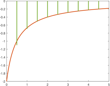
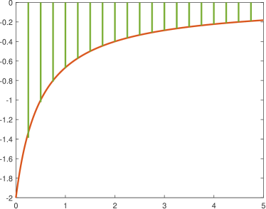
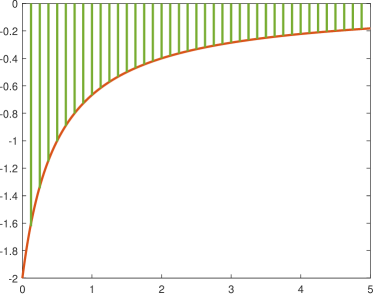
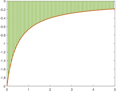
Figure 1. Comparison between $\overset{\ \curlyvee}{f^{T}}$ and $\overset{\ \curlyvee}{f}$ when $f=\frac{-4\sqrt{2\pi}}{1+2t}$.

Upper left: $T=\pi$. Upper right: $T=2\pi$. Lower left: $T=4\pi$. Lower right: $T=8\pi$.

Example 8.5.

We can further generalize the measure in the example above to the following: let $\mu=m+\beta\pi\delta_{0}$, then

$$f(t)=-\frac{\beta}{1+\beta t}$$

and

$$\overset{\ \curlywedge}{f}(z)=\frac{\beta i}{2z+\beta i}.$$

The traditionally studied $(a,b)-$pair can be recovered from $\overset{\ \curlywedge}{f}$ as well:

$$a_{\infty}(z)=\frac{2z+\beta i}{2z},\quad b_{\infty}(z)=\frac{\beta i}{2z}.$$

References

• [Car66] L. Carleson “On convergence and growth of partial sums of Fourier series” In Acta Mathematics 116, 1966, pp. 135–157 DOI: https://doi.org/10.1007/BF02392815
• [deB68] L. deBranges “Hilbert spaces of entire functions” Prentice-Hall, 1968
• [Den06] S.A. Denisov “Continuous analogs of polynomials orthogonal on the unit circle and Krein systems” 54517 In International Mathematics Research Surveys 2006, 2006, pp. 426–447 DOI: 10.1155/IMRS/2006/54517
• [Dym70] H. Dym “An introduction to de Branges spaces of entire functions with applications to differential equations of the Sturm-Liouville type” In Advances in Mathematics 5.3, 1970, pp. 395–471 DOI: https://doi.org/10.1016/0001-8708(70)90011-3
• [MP23] N. Makarov and A. Poltoratski “Etudes for the inverse spectral problem” In Journal of the London Mathematical Society 108.3, 2023, pp. 916–977 DOI: https://doi.org/10.1112/jlms.12772
• [MPS] N. Makarov, A. Poltoratski and M. Sodin “Lectures on linear complex analysis” unpublished lecture notes
• [MTT02] C. Muscalu, T. Tao and C. Thiele “A Carleson type theorem for a Cantor group model of the scattering transform” In Nonlinearity 16.1, 2002, pp. 219–246 DOI: 10.1088/0951-7715/16/1/314
• [Pol15] A. Poltoratski “Toeplitz Approach to Problems of the Uncertainty Principle”, CBMS series Providence, Rhode Island: American Mathematical Society, 2015
• [Pol23] A. Poltoratski “Pointwise convergence of the non-linear Fourier transform” In Annals of Mathematics To appear, 2023
• [PS06] A. Poltoratski and D. Sarason “Aleksandrov-Clark measures” In Contemporary Mathematics 393 Providence, Rhode Island: American Mathematical Society, 2006, pp. 1–14 DOI: http://dx.doi.org/10.1090/conm/393
• [PZ23] A. Poltoratski and A.R. Zhang “Periodic approximations in inverse spectral problems for canonical Hamiltonian systems” In Journal of Functional Analysis 284.11, 2023 DOI: https://doi.org/10.1016/j.jfa.2023.109883
• [Rem18] C. Remling “Spectral Theory of Canonical Systems” 70, De Gruyter Studies in Mathematics De Gruyter, 2018
• [Rom14] R. Romanov “Canonical Systems and de Branges Spaces”, 2014 URL: https://arxiv.org/abs/1408.6022
• [Sil17] D. Silva “Inequalities in nonlinear Fourier analysis”, 2017 URL: https://www.math.tecnico.ulisboa.pt/~oliveiraesilva/attachments/CIM.pdf
• [Tao02] T. Tao “An introduction to the nonlinear Fourier transform”, 2002 URL: http://www.math.ucla.edu/~tao/preprints/Expository/
• [TT12] T. Tao and C. Thiele “Nonlinear Fourier Analysis, IAS/Park City Graduate Summer School”, 2003, 2012 URL: https://arxiv.org/abs/1201.5129
• [TTT] T. Tao, C. Thiele and Y-J. Tsai “The nonlinear Fourier transform” URL: http://131.220.132.179/people/thiele/teaching/2012NLFT/chapter.pdf