Heat kernel gradient estimates for the Vicsek set

Abstract

We prove pointwise and $L^{p}$ gradient estimates for the heat kernel on the bounded and unbounded Vicsek set and applications to Sobolev inequalities are given. We also define a Hodge semigroup in that setting and prove estimates for its kernel.

1 Introduction

Heat kernel gradient estimates have proven to be a powerful and versatile tool in many different situations. For instance, they play an important role in the abstract Bakry-Émery theory of curvature bounds and functional inequalities, see [6]. They can also be used in harmonic analysis to prove boundedness of Riesz transforms, see [4, 14, 11] and in Riemannian and sub-Riemannian geometry to prove Sobolev and isoperimetric inequalities, see [9, 13, 29, 23].

On a complete Riemannian manifold, if we denote by $p_{t}$ the heat kernel, $d$ the Riemannian distance, and $\mu(B(x,\sqrt{t})$ the Riemannian volume measure of a geodesic ball with center $x$ and radius $\sqrt{t}$, then the Gaussian heat kernel estimates

$$\frac{c_{1}}{\mu(B(x,\sqrt{t}))}\exp\left(-c_{2}\frac{d(x,y)^{2}}{t}\right)\leq p_{t}(x,y)\leq\frac{c_{3}}{\mu(B(x,\sqrt{t}))}\exp\left(-c_{4}\frac{d(x,y)^{2}}{t}\right)$$ (1)

are equivalent to the combination of the volume doubling property and the 2-Poincaré inequality, see the celebrated works [21, 26]. However the matching gradient estimate

$$|\nabla_{x}p_{t}(x,y)|\leq\frac{C}{\sqrt{t}\mu(B(x,\sqrt{t}))}\exp\left(-c\frac{d(x,y)^{2}}{t}\right)$$ (2)

does not always follow from (1) and requires different assumptions on the manifold, like the Ricci curvature being non-negative, see [24]. The heat kernel Gaussian estimates (1) and corresponding gradient estimates (2) can more generally be studied in metric measure spaces and Dirichlet spaces which admit a carré du champ operator $\Gamma(f)$ which is used as a substitute to $|\nabla f|^{2}$, see for instance [16] and references therein.

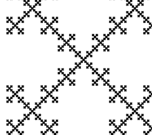
Figure 1: A part of an infinite, or unbounded, Vicsek set.

In a recent work [19], heat kernel gradient estimates have been obtained on some fractal-like cable systems for which the heat kernel has Gaussian estimates in small time and sub-Gaussian estimates in large time. In the present paper, we are interested in proving heat kernel gradient estimates in a metric measure space $(X,d,\mu)$, the unbounded Vicsek set (Figure 1), for which the heat kernel has the following sub-Gaussian estimates for every $t>0$:

$$\frac{c_{1}}{t^{d_{h}/d_{w}}}\exp\left(-c_{2}\Bigl{(}\frac{d(x,y)^{d_{w}}}{t}\Bigr{)}^{\frac{1}{d_{w}-1}}\right)\leq p_{t}(x,y)\leq\frac{c_{3}}{t^{d_{h}/d_{w}}}\exp\left(-c_{4}\Bigl{(}\frac{d(x,y)^{d_{w}}}{t}\Bigr{)}^{\frac{1}{d_{w}-1}}\right).$$

The parameter $d_{h}=\frac{\log 5}{\log 3}$ is the Hausdorff dimension of the metric space $(X,d)$, $\mu$ the Hausdorff measure and $d_{w}=d_{h}+1>2$ is a parameter which is called the walk dimension. Our interest in the Vicsek set comes from the fact that it provides a simple example of a space with sub-Gaussian heat kernel estimates and which does not admit a carré du champ operator. In such settings, heat kernel gradient estimates have never been obtained.

A first key point is to understand what a gradient estimate means in that setting. Despite the lack of a carré du champ operator, we recently introduced in [10] a notion of weak gradient $\partial$ on the Vicsek set. The key property that allows to define this gradient is that the Vicsek set is a metric tree. Intuitively, the gradient is defined on a dense but zero Hausdorff measure subset of the Vicsek set, the so-called skeleton $\mathcal{S}$, through the fundamental theorem of calculus:

$$f(x)-f(o)=\int_{\gamma}\partial f$$

where $o$ is the root of the Vicsek set and $\gamma$ the unique geodesic between $o$ and $x$. The function $\partial f$ can then be seen as a function on $\mathcal{S}$ which is locally integrable with respect to some measure $\nu$ on $\mathcal{S}$. It is worth noting, and at the heart of the many difficulties arising in our analysis, that due to the fractal nature of the Vicsek set, the measure $\nu$ is singular with respect to the measure $\mu$. More precisely, $\nu$ is supported on one-dimensional sets while $\mu$ which is the Hausdorff measure is supported on $d_{h}$ dimensional sets.

The first main result of the paper is the following theorem, see Proposition 3.5.

Theorem.

In the unbounded Vicsek set, the heat kernel $p_{t}(x,y)$ satisfies the following gradient estimate

$$|\partial_{x}p_{t}(x,y)|\leq\frac{C}{t^{1/d_{w}}}p_{ct}(x,y),\quad t>0.$$ (3)

The key idea and novelty in this estimate is to prove a substantial improvement of the weak Bakry-Émery estimates for the semigroup that were first obtained in [2], see Theorem 3.3. After proving the pointwise gradient estimate, we will shift our focus to the study of $L^{p}$ gradient bounds for the heat semigroup $P_{t}$ and obtain the following $L^{q}\to L^{p}$ gradient estimate. That is, let $1\leq q\leq p\leq+\infty$, then for every $f\in L^{q}$ and $t>0$,

$$\|\partial P_{t}f\|_{L^{p}(\mathcal{S},\nu)}\leq\frac{C}{t^{\left(1-\frac{1}{p}-\frac{1}{q}\right)\frac{1}{d_{w}}+\frac{1}{q}}}\|f\|_{L^{q}(X,\mu)}.$$ (4)

As an application of the heat kernel gradient estimates (4) we prove the following family of Nash inequalities

$$\|f\|_{L^{p}(X,\mu)}\leq C\|\partial f\|_{L^{p}(\mathcal{S},\nu)}^{\theta}\|f\|^{1-\theta}_{L^{1}(X,\mu)},\quad p>1,$$

where $\theta=\frac{(p-1)(d_{w}-1)}{pd_{w}-1}$.

In the second part of the paper we prove the existence of a semigroup $\vec{P_{t}}$ on $L^{2}(\mathcal{S},\nu)$ that satisfies the intertwining

$$\partial P_{t}=\vec{P_{t}}\partial.$$

By an analogy with the situation on Riemannian manifolds, we call $\vec{P_{t}}$ the Hodge semigroup. Our main result concerning the Hodge semigroup is the following, see Theorem 4.2.

Theorem.

The Hodge semigroup $\vec{P}_{t}$ admits a kernel $\vec{p}_{t}(x,y)$ that satisfies the estimate

$$|\vec{p}_{t}(x,y)|\leq\frac{C}{t^{1/d_{w}}}\exp\biggl{(}-c\Bigl{(}\frac{d(x,y)^{d_{w}}}{t}\Bigr{)}^{\frac{1}{d_{w}-1}}\biggr{)},\quad t>0.$$

Finally in the last part of the paper we show how the previous results can appropriately be modified if the underlying space is the bounded Vicsek set.

Let us point out that for simplicity of the presentation, we restrict our analysis to the planar Vicsek set. However our definitions and results trivially extend to the higher dimensional Vicsek sets. More generally, it appears reasonable to infer that our approach is general and might be extended to a large class of volume doubling metric trees which are increasing limits of cable systems trees. This will possibly be investigated in a later work.

Notations:

Throughout the paper, we use the letters $c,C,c_{1},c_{2},c_{3},c_{4}$ to denote positive constants which may vary from line to line.

2 Preliminaries

2.1 Vicsek set

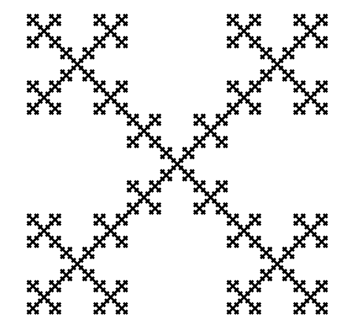
Figure 2: Bounded Vicsek set $K$

Let $q_{1}=(0,0)$ be the center of of the unit square in the plane and let $q_{2}=(-\sqrt{2}/2,\sqrt{2}/2)$, $q_{3}=(\sqrt{2}/2,\sqrt{2}/2)$ , $q_{4}=(\sqrt{2}/2,-\sqrt{2}/2)$, and $q_{5}=(-\sqrt{2}/2,-\sqrt{2}/2)$ be the 4 corners of the square. Define $\psi_{i}(z)=\frac{1}{3}(z-q_{i})+q_{i}$ for $1\leq i\leq 5$. The Vicsek set $K$ is the unique non-empty compact set such that

$$K=\bigcup_{i=1}^{5}\psi_{i}(K)$$

and the unbounded Vicsek set $X$ is defined by

$$X=\bigcup_{m=1}^{\infty}3^{m}K.$$

Let $W_{0}=\{q_{1},q_{2},q_{3},q_{4},q_{5}\}$. We define a sequence of sets of vertices $\{W_{n}\}_{n\geq 0}$ inductively by

$$W_{n+1}=\bigcup_{i=1}^{5}\psi_{i}(W_{n})\subset K.$$

By definition, a cable system with vertices in $W_{n}$ is a union of segments, called edges, whose extremities are in $W_{n}$. The unique connected cable system with vertices in $W_{n}$ and included in $K$ will be denoted $\bar{W}_{n}$.

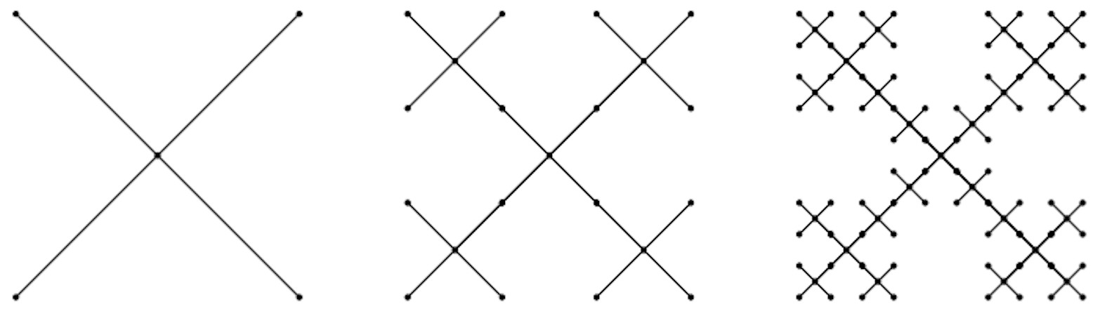
Figure 3: Cable systems $\bar{W}_{0}$, $\bar{W}_{1}$ and $\bar{W}_{2}$

We will denote

$$V_{n}=\bigcup_{m\geq 1}3^{m-n}W_{m},\quad\bar{V}_{n}=\bigcup_{m\geq 1}3^{m-n}\bar{W}_{m}$$

The set

$$\mathcal{S}=\bigcup_{n\geq 0}\bar{V}_{n}$$

is called the skeleton of $X$, it is a dense subset in $X$. We have then a natural sequence of cable systems $\{\bar{V}_{n}\}_{n\geq 0}$ whose edges have length $3^{-n}$ and whose set of vertices is $V_{n}$.

If $u,v$ are adjacent vertices in $\bar{V}_{n}$ connected by an edge, we will write $u\sim v$ and say that $u\leq v$ if the geodesic distance from the center $q_{1}=(0,0)$ to $u$ in $\bar{V}_{n}$ is less than the geodesic distance from $q_{1}$ to $v$. We will denote by $\mathbf{e}(u,v)$ the unique edge in $\bar{V}_{n}$ connecting $u$ to $v$.

We note that $\bar{V}_{n}$ is a metric tree when equipped of the geodesic distance. Given any $u,v\in\bar{V}_{n}$, we will denote by $\gamma(u,v)$ the unique geodesic in $\bar{V}_{n}$ connecting $u$ to $v$.

2.2 Geodesic distance and measures

On $X$, we will consider the geodesic distance $d$. More precisely, for $x,y\in X$, the distance $d(x,y)$ is defined as the infimum of the length of the rectifiable curves $\gamma:[0,1]\to\mathbb{R}^{2}$ such that $\gamma(0)=x$, $\gamma(1)=y$ and $\gamma(s)\in X$ for every $s\in[0,1]$. Note that the metric space $(X,d)$ is a metric tree.

The Hausdorff measure $\mu$ of $(X,d)$ is the unique measure on $X$ such that for every $i_{1},\cdots,i_{n}\in\{1,2,3,4,5\}$ and $m\geq 0$

$$\mu(3^{m}\psi_{i_{1}}\circ\cdots\circ\psi_{i_{n}}(K))=5^{m-n}.$$

The Hausdorff dimension of $X$ is then $d_{h}=\frac{\log 5}{\log 3}$ and the metric space $(X,d)$ is $d_{h}$-Ahlfors regular in the sense that there exist constants $c,C>0$ such that for every $x\in K$, $r\geq 0$,

$$c\,r^{d_{h}}\leq\mu(B(x,r))\leq Cr^{d_{h}},$$

where $B(x,r)=\left\{y\in X,d(x,y)\leq r\right\}$ denotes the closed ball with center $x$ and radius $r$.

There is also a reference measure $\nu$ on the skeleton $\mathcal{S}$, the Lebesgue measure. It is characterized by the property that for every edge $\mathbf{e}$ in $\bar{V}_{n}$ connecting two neighboring vertices:

$$\nu(\mathbf{e})=3^{-n}.$$

The measure $\nu$ is not finite (because the skeleton obviously has infinite length) but it is $\sigma$-finite on the $\sigma$-field generated by the $\mathbf{e}(x,y)$, $x,y\in V_{n}$, $x\sim y$, $n\geq 0$. The measure $\nu$ is not a Radon measure neither since the measure of any ball with positive radius is infinite. From the definition, it is also clear that $\nu$ is singular with respect to the Hausdorff measure $\mu$ since the skeleton has $\mu$-measure zero.

2.3 Weak gradients, Sobolev spaces

We denote by $L^{1}_{\mathrm{l}oc}(\mathcal{S},\nu)$ the space of measurable functions with respect to the $\sigma$-field generated by the $\mathbf{e}(x,y)$, $x,y\in V_{n}$, $x\sim y$, $n\geq 0$ and $\nu$-integrable on each of those $\mathbf{e}(x,y)^{\prime}s$.

Definition 2.1.

Let $f\in C(X)$. We say that $f$ admits a weak gradient if there exists a measurable function $\partial f\in L^{1}_{\mathrm{l}oc}(\mathcal{S},\nu)$ such that that for every $n$ and for every adjacent $u,v\in V_{n}$ with $u\leq v$

$$f(v)-f(u)=\int_{\mathbf{e}(u,v)}\partial fd\nu.$$ (5)

The set $\bar{V}_{n}$ is a cable system. As such, see for instance Section 5.1 in [12], one can see any continuous function on $\bar{V}_{n}$ as a collection of functions $(f_{\mathbf{e}})_{\mathbf{e}\in E_{n}}$ where $E_{n}$ is the set of edges of $\bar{V}_{m}$ and $f_{\mathbf{e}}:\left[0,3^{-n}\right]\to\mathbb{R}$ is a continuous function with the appropriate boundary conditions. For $f\in C(X)$ let us denote $f^{n}=f_{|\bar{V}_{n}}$. One can then see that $f$ admits a weak gradient if and only if we have for all $\mathbf{e}$ in $E_{n}$, $f^{n}_{\mathbf{e}}\in W^{1,1}\left(\left[0,3^{-n}\right]\right)$, where for an interval $I\subset\mathbb{R}$, $W^{1,1}(I)$ is the usual $(1,1)$ Sobolev space for the Lebesgue measure. The following proposition is immediate from properties of weak derivatives on the real line.

Proposition 2.2 (Chain, Leibniz, and scaling rules).

1. Let $f\in C(X)$ and let $\Phi$ be a $C^{1}$ function on $\mathbb{R}$. If $f$ admits a weak gradient, then $\Phi(f)$ admits a weak gradient and

   $$\partial\Phi(f)=\Phi^{\prime}(f)\partial f.$$

2. Let $f,g\in C(X)$. If $f$ and $g$ admit weak gradients, then $fg$ admits a weak gradient and

   $$\partial(fg)=f\partial g+g\partial f.$$

3. Let $f\in C(X)$. If $f$ admits a weak gradient, then for every $i_{1},\cdots,i_{n}\in\{1,2,3,4,5\}$, the function $f\circ\psi_{i_{1}}\circ\cdots\circ\psi_{i_{n}}$ admits a weak gradient and

   $$\partial(f\circ\psi_{i_{1}}\circ\cdots\circ\psi_{i_{n}})=3^{-n}(\partial f)\circ\psi_{i_{1}}\circ\cdots\circ\psi_{i_{n}}.$$

Definition 2.3.

Let $1\leq p\leq\infty$. For $f\in C(X)$, we say that $f\in D^{1,p}(X)$ if it admits a weak gradient $\partial f\in L^{p}(\mathcal{S},\nu)$. We will denote $W^{1,p}(X)=L^{p}(X,\mu)\cap D^{1,p}(X)$.

The seminorm on $D^{1,p}(X)$ is defined by

$$\|f\|_{D^{1,p}(X)}:=\|\partial f\|_{L^{p}(X,\nu)}.$$

One can see that $D^{1,\infty}(X)$ is the space of Lipschitz continuous functions on $X$ and that $\|\partial f\|_{L^{\infty}(X,\nu)}$ is the Lipschitz constant $\mathrm{Lip}(f)$ of $f$. We refer to [10, Section 3] for equivalent characterizations in the compact Vicsek set of the space $W^{1,p}(X)$, in terms of Korevaar-Schoen-Sobolev seminorms and discrete $p$-energies.

We note that it easily follows from the definition that if $f\in D^{1,p}(X)$, then for every $x,y\in\mathcal{S}$

$$|f(x)-f(y)|\leq\int_{\gamma(x,y)}|\partial f|d\nu,$$

where we recall that $\gamma(x,y)$ denotes the unique geodesic in $\mathcal{S}$ connecting $x$ to $y$. From Hölder’s inequality we get that for every $x,y\in\mathcal{S}$

$$|f(x)-f(y)|\leq d(x,y)^{1-\frac{1}{p}}\left(\int_{\gamma(x,y)}|\partial f|^{p}d\nu\right)^{p}\leq d(x,y)^{1-\frac{1}{p}}\|\partial f\|_{L^{p}(X,\nu)}^{p}.$$

This inequality then holds for every $x,y\in X$ since $f$ is continuous and $\mathcal{S}$ is dense in $X$. Therefore for $p>1$, any $f\in D^{1,p}(X)$ is $1-\frac{1}{p}$ Hölder continuous.

We now collect some basic properties of the weak gradient that will be important in the sequel.

Proposition 2.4.

Let $1<p\leq+\infty$. The operator $\partial:W^{1,p}(X)\to L^{p}(X,\nu)$ is closed.

Proof.

Let $f_{n}$ be a sequence in $W^{1,p}(X)$ that converges to some $f$ in $L^{p}(X,\mu)$ and such that $\partial f_{n}$ converges in $L^{p}(X,\nu)$ to some $g\in L^{p}(X,\nu)$. We have for every $n$ and for every $u,v\in\mathcal{S}$

$$|f_{n}(v)-f_{n}(u)|\leq\int_{\gamma(u,v)}\left|\partial f_{n}\right|d\nu\leq d(u,v)^{1-\frac{1}{p}}\left(\int_{\gamma(u,v)}|\partial f_{n}|^{p}d\nu\right)^{1/p}\leq d(u,v)^{1-\frac{1}{p}}\|\partial f_{n}\|_{L^{p}(X,\nu)}.$$

Since $\partial f_{n}$ converges in $L^{p}(X,\nu)$, there exists therefore a constant $C>0$ such that for every $n$ and for every $u,v\in\mathcal{S}$

$$|f_{n}(v)-f_{n}(u)|\leq Cd(u,v)^{1-\frac{1}{p}}.$$

By continuity of $f_{n}$ and density in $X$ of $\mathcal{S}$, this inequality holds true for every $u,v\in X$. Using the assumed convergence of $f_{n}$ to $f$ in $L^{p}(X,\mu)$ and Arzela-Ascoli theorem we deduce that given $u,v\in V_{m}$ with $u,v$ adjacent and $u\leq v$, there exists a subsequence $f_{n_{k}}$ such that $f_{n_{k}}$ converges uniformly to $f$ on $\mathbf{e}(u,v)$. Since

$$f_{n_{k}}(v)-f_{n_{k}}(u)=\int_{\mathbf{e}(u,v)}\partial f_{n_{k}}d\nu$$

one deduces by taking the limit that

$$f(v)-f(u)=\int_{\mathbf{e}(u,v)}gd\nu.$$

Since $g\in L^{p}(X,\nu)$ one deduces that $f\in W^{1,p}(X)$ and that $g=\partial f$. ∎

Proposition 2.5.

Let $1<p\leq+\infty$. The operator $\partial:D^{1,p}(X)\to L^{p}(\mathcal{S},\nu)$ is surjective.

Proof.

Let $\omega\in L^{p}(\mathcal{S},\nu)$. For $v\in\mathcal{S}$, let

$$f(v)=\int_{\gamma(0,v)}\omega(x)d\nu(x),$$

where we recall that $\gamma(0,v)$ denotes the unique geodesic path from $0$ to $v$. As before, one can see that for every $u,v\in\mathcal{S}$,

$$|f(v)-f(u)|\leq d(u,v)^{1-1/p}\left(\int_{\mathcal{S}}|\omega|^{p}d\nu\right)^{1/p}.$$

Therefore $f$ admits a unique Hölder continuous extension to $X$ that we still denote by $f$. We have then $f\in D^{1,p}(X)$ and $\partial f=\omega$. ∎

The following notion of piecewise affine function will play an important role.

Definition 2.6.

A continuous function $\Phi:X\to\mathbb{R}$ is called $n$-piecewise affine, if there exists $n\geq 0$ such that $\Phi$ is piecewise affine on the cable system $\bar{V}_{n}$ (i.e linear between the vertices of $\bar{V}_{n}$) and constant on any connected component of $\bar{V}_{m}\setminus\bar{V}_{n}$ for every $m>n$. In other words, a continuous function $\Phi:X\to\mathbb{R}$ is $n$-piecewise affine if

$$\Phi(x)=\Phi(0)+\int_{\gamma(0,x)}\eta d\nu,\quad x\in\mathcal{S},$$

where $\eta$ is a function on $\mathcal{S}$ which is supported on $\bar{V}_{n}$ and which is constant on each of the edges of $\bar{V}_{n}$.

We have the following approximation result.

Lemma 2.7.

Let $1\leq p<+\infty$. For any $\eta\in L^{p}(\mathcal{S},\nu)\cap L^{\infty}(\mathcal{S},\nu)$, there exists a sequence $\phi_{n}\in W^{1,p}(X)$ such that

1. $\partial\phi_{n}$ is bounded in $L^{p}(\mathcal{S},\nu)$;

2. $\partial\phi_{n}\to\eta$ in $L^{q}(\mathcal{S},\nu)$, $p<q<+\infty$;

3. $\|\partial\phi_{n}\|_{L^{\infty}(\mathcal{S},\nu)}\leq 2\|\eta\|_{L^{\infty}(\mathcal{S},\nu)}$.

Proof.

We first construct a convenient family of cutoff functions. Consider the unique 1-piecewise affine function $h$ on $X$ which is equal to 1 on the vertices $\frac{1}{3}W_{0}$ and zero on all of the other vertices of $V_{1}$. Let

$$h_{n}(x)=h(x/3^{n}),\,x\in X.$$

We have then for every $x\in X$, $h_{n}(x)\to 1$ when $n\to\infty$ and moreover

$$|\partial h_{n}(x)|\leq 3^{-n}1_{3^{n}\bar{W}_{0}\setminus 3^{n-1}\bar{W}_{0}}(x).$$ (6)

For $\eta\in L^{p}(\mathcal{S},\nu)\cap L^{\infty}(\mathcal{S},\nu)$, we define

$$\phi_{n}(x)=h_{n}(x)\int_{\gamma(0,x)}\eta d\nu,\quad x\in\mathcal{S}.$$

By continuity, $\phi_{n}$ admits an extension to $X$, which is still denoted by $\phi_{n}$. Since $\phi_{n}$ is continuous and compactly supported, we have $\phi_{n}\in L^{p}(X,\mu)$.

Next we observe that for $\nu$ a.e. $x\in\mathcal{S}$

$$\partial\phi_{n}(x)=\partial h_{n}(x)\int_{\gamma(0,x)}\eta d\nu+h_{n}(x)\eta(x).$$

Since $\eta\in L^{q}(\mathcal{S},\nu)$ for $q\geq p$, it is easy to see that $h_{n}\eta\to\eta$ in $L^{q}(\mathcal{S},\nu)$ when $q\geq p$. On the other hand, we have from (6) and Hölder’s inequality that

$$\int_{\mathcal{S}}\left|\partial h_{n}(x)\int_{\gamma(0,x)}\eta d\nu\right|^{q}d\nu(x) \leq\int_{\mathcal{S}}\left(3^{-n}1_{3^{n}\bar{W}_{0}\setminus 3^{n-1}\bar{W}_{0}}(x)\right)^{q}\left(\|\eta\|_{L^{p}(\mathcal{S},\nu)}d(0,x)^{1-\frac{1}{p}}\right)^{q}d\nu(x)$$

$$\leq 3^{-nq}\|\eta\|_{L^{p}(\mathcal{S},\nu)}^{q}\int_{\mathcal{S}}1_{3^{n}\bar{W}_{0}\setminus 3^{n-1}\bar{W}_{0}}(x)d(0,x)^{q-\frac{q}{p}}d\nu(x)$$

$$\leq 3^{-nq}\|\eta\|_{L^{p}(\mathcal{S},\nu)}^{q}3^{n\left(q-\frac{q}{p}\right)}\nu(3^{n}\bar{W}_{0}\setminus 3^{n-1}\bar{W}_{0})$$

$$\leq 3^{n\left(1-\frac{q}{p}\right)}\|\eta\|_{L^{p}(\mathcal{S},\nu)}^{q}.$$

Hence the integral is bounded for $p=q$, and converges to zero when $n\to+\infty$ for $p<q<\infty$. We deduce that $\partial\phi_{n}\to\eta$ in $L^{q}(\mathcal{S},\nu)$ for $p<q<+\infty$, and $\partial\phi_{n}$ is bounded in $L^{p}(\mathcal{S},\nu)$. So claims $(\mathrm{i})$ and $(\mathrm{ii})$ hold.

Finally, we have $\nu$ a.e. $x\in\mathcal{S}$

$$|\partial\phi_{n}(x)| \leq|\partial h_{n}(x)|\,\left|\int_{\gamma(0,x)}\eta d\nu\right|+h_{n}(x)|\eta(x)|$$

$$\leq 3^{-n}1_{3^{n}\bar{W}_{0}\setminus 3^{n-1}\bar{W}_{0}}(x)d(0,x)\|\eta\|_{L^{\infty}(\mathcal{S},\nu)}+\|\eta\|_{L^{\infty}(\mathcal{S},\nu)}$$

$$\leq 2\|\eta\|_{L^{\infty}(\mathcal{S},\nu)}.$$

This concludes $(\mathrm{iii})$ and we finish the proof. ∎

Proposition 2.8.

Let $1<p<+\infty$. The range of the operator $\partial:W^{1,p}(X)\to L^{p}(\mathcal{S},\nu)$ is dense in $L^{p}(\mathcal{S},\nu)$.

Proof.

Let $1<p<+\infty$. Since $L^{1}(\mathcal{S},\nu)\cap L^{\infty}(\mathcal{S},\nu)$ is dense in $L^{p}(\mathcal{S},\nu)$, it is enough to prove that the range of $\partial$ is $L^{p}$ dense in $L^{1}(\mathcal{S},\nu)\cap L^{\infty}(\mathcal{S},\nu)$, which immediately follows from Lemma 2.7 $(\mathrm{ii})$. ∎

3 Heat kernel gradient bounds

3.1 Dirichlet form, Heat kernel

We now introduce the canonical Dirichlet form on $X$ and recall some of the basic properties of its associated heat kernel with respect to the measure $\mu$. For $f,g\in W^{1,2}(X)$, define

$$\mathcal{E}(f,g)=\int_{\mathcal{S}}\partial f\,\partial g\,d\nu.$$

We note that if $\Phi:X\to\mathbb{R}$ is $n$-piecewise affine, then for every $m>n$

$$\mathcal{E}(\Phi,\Phi)=\frac{1}{2}3^{m}\sum_{x,y\in V_{m},x\sim y}|\Phi(x)-\Phi(y)|^{2}.$$

Using then known result about Dirichlet forms as limits of self-similar energies on infinite nested fractals as in [7, Theorem 7.14] and [20, Theorem 2.7] (see also Theorem 2.9 in [10]), we have the following result.

Theorem 3.1.

The quadratic form $\mathcal{E}$ with domain $W^{1,2}(X)$ is a strongly local and regular Dirichlet form in $L^{2}(X,\mu)$. A core for $\mathcal{E}$ is the set of compactly supported piecewise affine functions. Moreover, for every $f\in W^{1,2}(X)$

$$\mathcal{E}(f,f)=\lim_{m\to+\infty}\frac{1}{2}3^{m}\sum_{x,y\in V_{m},x\sim y}|f(x)-f(y)|^{2}.$$

Let $\Delta$ be the generator of $(\mathcal{E},W^{1,2}(X))$ in $L^{2}(X,\mu)$, i.e., for $f\in\mathrm{dom}(\Delta)$ and $g\in W^{1,2}(X)$,

$$\int_{\mathcal{S}}\partial f\partial gd\nu=-\int_{X}g\Delta fd\mu.$$

The associated heat semigroup $(P_{t})_{t\geq 0}=(e^{t\Delta})_{t\geq 0}$ admits a continuous heat kernel with respect to the Hausdorff measure $\mu$ that we denote by $p_{t}(x,y)$. The heat kernel $p_{t}(x,y)$ satisfies sub-Gaussian estimates, see [7, Theorem 8.18] and [20, Theorem 1]. More precisely, for every $(x,y)\in X\times X$ and $t>0$

$$c_{1}t^{-d_{h}/d_{w}}\exp\biggl{(}-c_{2}\Bigl{(}\frac{d(x,y)^{d_{w}}}{t}\Bigr{)}^{\frac{1}{d_{w}-1}}\biggr{)}\leq p_{t}(x,y)\leq c_{3}t^{-d_{h}/d_{w}}\exp\biggl{(}-c_{4}\Bigl{(}\frac{d(x,y)^{d_{w}}}{t}\Bigr{)}^{\frac{1}{d_{w}-1}}\biggr{)},$$ (7)

where $d_{w}:=d_{h}+1$ is often called the walk dimension. Those sub-Gaussian estimates easily imply (see Lemma 2.3 in [2]) that for every $\kappa\geq 0$, there are constants $c,C>0$ so that for every $x,y\in X$, and $t>0$

$$d(x,y)^{\kappa}p_{t}(x,y)\leq Ct^{\kappa/d_{w}}p_{ct}(x,y).$$ (8)

For later use we record the following bound which classically follows from the heat kernel estimates, see for instance [18, Corollary 5].

Lemma 3.2.

There exist constants $c,C>0$ such that for every $t>0$ and $x,y\in X$,

$$|\partial_{t}p_{t}(x,y)|\leq Ct^{-1-d_{h}/d_{w}}\exp\biggl{(}-c\Bigl{(}\frac{d(x,y)^{d_{w}}}{t}\Bigr{)}^{\frac{1}{d_{w}-1}}\biggr{)}.$$ (9)

3.2 Heat kernel Lipschitz estimates and gradient bounds

We start with the following Lipschitz estimate for the heat kernel.

Theorem 3.3.

There exist constants $c,C>0$ such that for every $x,y,z\in X$, and $t>0$

$$|p_{t}(z,x)-p_{t}(z,y)|\leq C\frac{d(x,y)}{t^{1/d_{w}}}(p_{ct}(z,x)+p_{ct}(z,y)).$$ (10)

Proof.

Denote by

$$g_{\lambda}(x,y)=\int_{0}^{+\infty}e^{-\lambda t}p_{t}(x,y)dt,\quad\lambda>0,$$

the resolvent kernel of $\Delta$, i.e.,

$$G_{\lambda}f(x)=(\Delta-\lambda)^{-1}f(x)=\int_{X}g_{\lambda}(x,y)f(y)d\mu(y),\quad f\in L^{2}(X,\mu).$$

From [7, Theorem 3.40], one has the following estimate

$$|g_{\lambda}(z,x)-g_{\lambda}(z,y)|\leq C\lambda^{1-d_{h}/d_{w}}d(x,y)(g_{\lambda}(z,x)+g_{\lambda}(z,y)).$$

Integrating the estimate yields that for $f\in L^{2}(X,\mu)$

$$|G_{\lambda}f(x)-G_{\lambda}f(y)|\leq C\lambda^{1-d_{h}/d_{w}}d(x,y)(G_{\lambda}|f|(x)+G_{\lambda}|f|(y)).$$

Thus, for any $f\in\mathrm{dom}(\Delta)$ and $\lambda>0$

$$|f(x)-f(y)|\leq C\lambda^{1-d_{h}/d_{w}}d(x,y)(G_{\lambda}|(\Delta-\lambda)f|(x)+G_{\lambda}|(\Delta-\lambda)f|(y)).$$

We now apply this equality with $f=p_{t}(z,\cdot)$, this gives

$$|p_{t}(z,x)-p_{t}(z,y)|\leq C\lambda^{1-d_{h}/d_{w}}d(x,y)(G_{\lambda}|(\Delta-\lambda)p_{t}(z,\cdot)|(x)+G_{\lambda}|(\Delta-\lambda)p_{t}(z,\cdot)|(y)).$$

We then have from Lemma 3.2

$$G_{\lambda}|(\Delta-\lambda)p_{t}(z,\cdot)|(x) =\int_{X}g_{\lambda}(x,u)|(\Delta-\lambda)p_{t}(z,u)|d\mu(u)$$

$$\leq C\left(\lambda+\frac{1}{t}\right)\int_{X}g_{\lambda}(x,u)p_{c_{1}t}(z,u)d\mu(u),$$

and

$$\int_{X}g_{\lambda}(x,u)p_{c_{1}t}(z,u)d\mu(u) =\int_{0}^{+\infty}\int_{X}e^{-\lambda s}p_{s}(x,u)p_{c_{1}t}(z,u)d\mu(u)ds$$

$$=\int_{0}^{+\infty}e^{-\lambda s}p_{s+c_{1}t}(x,z)ds$$

$$\leq e^{c_{1}\lambda t}\int_{0}^{+\infty}e^{-\lambda u}p_{u}(x,z)du.$$

One now uses the estimate

$$\int_{0}^{+\infty}e^{-\lambda u}p_{u}(x,z)du\leq C\lambda^{\frac{d_{h}}{d_{w}}-1}e^{-c_{2}\lambda^{1/d_{w}}d(x,z)}.$$

which follows from the upper bound in (7) by integrating with respect to $\lambda$ (see [7, Proposition 3.28]). Therefore, we have

$$\int_{X}g_{\lambda}(x,u)p_{ct}(z,u)d\mu(u)\leq C\lambda^{\frac{d_{h}}{d_{w}}-1}e^{c_{1}\lambda t-c_{2}\lambda^{1/d_{w}}d(x,z)},$$

and conclude

$$|p_{t}(z,x)-p_{t}(z,y)|\leq Cd(x,y)\left(\lambda+\frac{1}{t}\right)\left(e^{c_{1}\lambda t-c_{2}\lambda^{1/d_{w}}d(x,z)}+e^{c_{1}\lambda t-c_{2}\lambda^{1/d_{w}}d(y,z)}\right).$$

Assume first $d(y,z)\geq d(x,z)$. One has then

$$|p_{t}(z,x)-p_{t}(z,y)|\leq Cd(x,y)\left(\lambda+\frac{1}{t}\right)e^{c_{1}\lambda t-c_{2}\lambda^{1/d_{w}}d(x,z)}.$$

If we choose $\lambda=\alpha\left(\frac{d(x,z)}{t}\right)^{\frac{d_{w}}{d_{w}-1}}$ with a constant $\alpha>0$ small enough such that $c_{2}\alpha^{1/d_{w}}-c_{1}\alpha>0$ (such difference is denoted by $c_{3}$), one obtains

$$|p_{t}(z,x)-p_{t}(z,y)| \leq Cd(x,y)\left(\left(\frac{d(x,z)}{t}\right)^{\frac{d_{w}}{d_{w}-1}}+\frac{1}{t}\right)e^{-c_{3}\Bigl{(}\frac{d(x,z)^{d_{w}}}{t}\Bigr{)}^{\frac{1}{d_{w}-1}}}$$

$$\leq\frac{C}{t}d(x,y)e^{-c_{4}\Bigl{(}\frac{d(x,z)^{d_{w}}}{t}\Bigr{)}^{\frac{1}{d_{w}-1}}}$$

$$\leq\frac{C}{t^{1-d_{h}/d_{w}}}d(x,y)p_{ct}(x,z),$$

where we used the fact that

$$d(x,z)^{\frac{d_{w}}{d_{w}-1}}e^{-c_{3}\Bigl{(}\frac{d(x,z)^{d_{w}}}{t}\Bigr{)}^{\frac{1}{d_{w}-1}}}\leq Ct^{\frac{1}{d_{w}-1}}e^{-c_{4}\Bigl{(}\frac{d(x,z)^{d_{w}}}{t}\Bigr{)}^{\frac{1}{d_{w}-1}}}.$$

Similarly, if $d(y,z)\geq d(x,z)$, one obtains

$$|p_{t}(z,x)-p_{t}(z,y)|\leq\frac{C}{t^{1-d_{h}/d_{w}}}d(x,y)p_{ct}(y,z)$$

and the conclusion follows. ∎

As a corollary, we get an improved weak Bakry-Émery estimate (compared to [2, Theorem 3.7]).

Corollary 3.4.

There exist constants $c,C>0$ such that for every $f\in L^{\infty}(X,\mu)$, $x,y\in X$ and $t>0$

$$|P_{t}f(x)-P_{t}f(y)|\leq C\frac{d(x,y)}{t^{1/d_{w}}}(P_{ct}|f|(x)+P_{ct}|f|(y)).$$

Therefore, there exist constants $c,C>0$ such that for every $f\in L^{\infty}(X,\mu)$, $\nu$ a.e. $x\in\mathcal{S}$ and every $t>0$

$$|\partial P_{t}f(x)|\leq\frac{C}{t^{1/d_{w}}}P_{ct}|f|(x).$$

Proof.

The first part of the corollary follows directly from the previous theorem. Indeed, for every $f\in L^{\infty}(X,\mu)$, $x,y\in X$ and $t>0$

$$|P_{t}f(x)-P_{t}f(y)| =\left|\int_{X}p_{t}(z,x)d\mu(z)-\int_{X}p_{t}(z,y)d\mu(z)\right|$$

$$\leq\int_{X}|p_{t}(z,x)-p_{t}(z,y)|\,|f(z)|d\mu(z)$$

$$\leq C\frac{d(x,y)}{t^{1/d_{w}}}\int_{X}(p_{ct}(z,x)+p_{ct}(z,y))|f(z)|d\mu(z)$$

$$\leq C\frac{d(x,y)}{t^{1/d_{w}}}(P_{ct}|f|(x)+P_{ct}|f|(y)).$$

For the second part, notice that for every $x,y\in\mathcal{S}$ such that $\gamma(x,y)$ does not intersect the center $0$ of $X$, one has

$$|P_{t}f(x)-P_{t}f(y)|=\left|\int_{\gamma(x,y)}\partial P_{t}f(u)d\nu(u)\right|.$$

One obtains therefore

$$\left|\int_{\gamma(x,y)}\partial P_{t}f(u)d\nu(u)\right|\leq C\frac{d(x,y)}{t^{1/d_{w}}}(P_{ct}|f|(x)+P_{ct}|f|(y)).$$

Since $P_{ct}|f|$ is continuous, it then easily follows from the Lebesgue differentiation theorem that for $\nu$ a.e. $x\in\mathcal{S}$ and every $t>0$

$$|\partial P_{t}f(x)|\leq\frac{C}{t^{1/d_{w}}}P_{ct}|f|(x).$$

∎

We also obtain the following gradient estimate for the heat kernel.

Proposition 3.5.

There exist $c,C>0$ such that for every $t>0$, $y\in X$, and $\nu$ a.e. $x\in\mathcal{S}$

$$|\partial_{x}p_{t}(x,y)|\leq\frac{C}{t^{1/d_{w}}}p_{ct}(x,y)$$

and such that for every $t>0$, $x\in X$, and $\nu$ a.e. $y\in\mathcal{S}$

$$|\partial_{y}p_{t}(x,y)|\leq\frac{C}{t^{1/d_{w}}}p_{ct}(x,y).$$

Proof.

This follows from Theorem 3.3 and the same arguments as in the proof of Corollary 3.4. ∎

Remark 3.6.

Using the sub-Gaussian upper bound (7) one can rewrite the gradient estimate in Proposition 3.5 as

$$|\partial_{x}p_{t}(x,y)|\leq\frac{C}{t}\exp\left(-c\Bigl{(}\frac{d(x,y)^{d_{w}}}{t}\Bigr{)}^{\frac{1}{d_{w}-1}}\right).$$ (11)

3.3 Continuity $L^{q}\to W^{1,p}$ of the heat semigroup

In the previous section we obtained pointwise gradient estimates for the heat kernel. The goal of this section is to obtain $L^{p}$ gradient bounds. Let us observe that one can not obtain integrated gradient estimates by simply integrating with respect to $\nu$ the upper bound (11). Indeed, since $\nu$ is not a Radon measure, for $\nu$ a.e. $x\in\mathcal{S}$ the function $y\to\exp\left(-c\Bigl{(}\frac{d(x,y)^{d_{w}}}{t}\Bigr{)}^{\frac{1}{d_{w}-1}}\right)$ is not in $L^{p}(\mathcal{S},\nu)$ for any $p\geq 1$. Instead we will obtain integrated gradient estimates using the co-differential operator and an associated Poincaré type inequality proved in the Proposition 3.8 below.

The co-differential is defined as the $L^{2}$ adjoint of the weak gradient $\partial$. This means that the operator $\partial^{*}$ is the densely defined operator from $L^{2}(\mathcal{S},\nu)\to L^{2}(X,\mu)$ with domain

$$\mathrm{dom}\,\partial^{*}:=\left\{\eta\in L^{2}(\mathcal{S},\nu):~{}\exists f\in L^{2}(X,\mu),~{}\text{with }\int_{\mathcal{S}}\eta\partial\phi d\nu=\int_{X}f\phi d\mu,\forall~{}\phi\in W^{1,2}(X)\right\}.$$

Given $\eta\in\mathrm{dom}\,\partial^{*}$, there is a unique $f\in L^{2}(X,\mu)$ that satisfies

$$\int_{\mathcal{S}}\eta\partial\phi d\nu=\int_{X}f\phi d\mu,\quad\forall~{}\phi\in W^{1,2}(X)$$

and we define then $\partial^{*}\eta=f$.

Lemma 3.7.

We have

$$\operatorname{dom}\Delta=\left\{u\in\operatorname{dom}\mathcal{E}~{}|~{}\partial u\in\operatorname{dom}\partial^{*}\right\},$$

and for $u\in\operatorname{dom}\Delta$,

$$\Delta u=-\partial^{*}\partial u.$$

Proof.

Observe that $u\in\operatorname{dom}\mathcal{E}$ is in $\operatorname{dom}\Delta$ if and only if $\mathcal{E}(u,\phi)=-\int_{X}\phi\Delta ud\mu$ for all $\phi\in W^{1,2}(X)$. Since

$$\mathcal{E}(u,\phi)=\int_{\mathcal{S}}\partial u\partial\phi d\nu,$$

the result follows. ∎

The co-differential satisfies the following inequality.

Proposition 3.8.

Let $\eta\in\mathrm{dom}\,\partial^{*}$ and $x_{0}\in X$. Assume that $\int_{X}d(x_{0},x)|\partial^{*}\eta|(x)d\mu(x)<\infty$ and $d(x_{0},x)|\eta(x)|\to 0$ as $d(x_{0},x)\to+\infty$. Then we have

$$\int_{\mathcal{S}}|\eta|d\nu\leq\int_{X}d(x_{0},x)|\partial^{*}\eta|(x)d\mu(x).$$

Proof.

We consider the sequence of cutoff functions $\{h_{n}\}_{n\geq 1}$ introduced in the proof of Lemma 2.7. Let now $\eta\in\mathrm{dom}\,\partial^{*}$ and $x_{0}\in X$ satisfy the assumptions of the proposition. For $n\geq 1$, we define

$$g_{n}(x)=h_{n}(x)\left(\int_{\gamma(0,x)}\frac{\eta(y)}{|\eta(y)|+1/n}d\nu(y)-\int_{\gamma(0,x_{0})}\frac{\eta(y)}{|\eta(y)|+1/n}d\nu(y)\right),\quad x\in\mathcal{S}$$

which we extend by continuity to $X$. The extension is still denoted by $g_{n}$ and it is easy to see that it satisfies for every $x\in X$

$$|g_{n}(x)|\leq d(x_{0},x),$$

because the function

$$x\to\int_{\gamma(0,x)}\frac{\eta(y)}{|\eta(y)|+1/n}d\nu(y)-\int_{\gamma(0,x_{0})}\frac{\eta(y)}{|\eta(y)|+1/n}d\nu(y)$$

is 1-Lipschitz and vanishes at $x_{0}$. Note also that $g_{n}$ is compactly supported and therefore in $L^{2}(X,\mu)$.

We have for $\nu$ a.e. $x\in X$

$$\partial g_{n}(x)=\varepsilon_{n}(x)+\frac{h_{n}(x)\eta(x)}{|\eta(x)|+1/n}.$$

where

$$\varepsilon_{n}(x)=\partial h_{n}(x)\left(\int_{\gamma(0,x)}\frac{\eta(y)}{|\eta(y)|+1/n}d\nu(y)-\int_{\gamma(0,x_{0})}\frac{\eta(y)}{|\eta(y)|+1/n}d\nu(y)\right).$$

We obtain therefore

$$\int_{\mathcal{S}}\frac{h_{n}(x)\eta(x)^{2}}{|\eta(x)|+1/n}d\nu(x) =\int_{\mathcal{S}}\partial g_{n}(x)\eta(x)d\nu(x)-\int_{\mathcal{S}}\varepsilon_{n}(x)\eta(x)d\nu(x)$$

$$=\int_{X}g_{n}(x)\partial^{*}\eta(x)d\mu(x)-\int_{\mathcal{S}}\varepsilon_{n}(x)\eta(x)d\nu(x).$$

This yields

$$\int_{\mathcal{S}}\frac{h_{n}(x)\eta(x)^{2}}{|\eta(x)|+1/n}d\nu(x) \leq\int_{X}|g_{n}(x)\partial^{*}\eta(x)|d\mu(x)+\int_{\mathcal{S}}|\varepsilon_{n}(x)||\eta(x)|d\nu(x)$$

$$\leq\int_{X}d(x_{0},x)|\partial^{*}\eta(x)|d\mu(x)+\int_{\mathcal{S}}|\partial h_{n}(x)|d(x_{0},x)|\eta(x)|d\nu(x),$$

where we used in the last inequality that

$$|\varepsilon_{n}(x)|\leq|\partial h_{n}(x)|d(x_{0},x).$$

Recall that $h_{n}\to 1$ as $n\to\infty$. By Fatou’s lemma, it therefore remains to prove that

$$\lim_{n\to+\infty}\int_{\mathcal{S}}|\partial h_{n}(x)|d(x_{0},x)|\eta(x)|d\nu(x)=0.$$

This simply follows from the fact that

$$\int_{\mathcal{S}}|\partial h_{n}(x)|d(x_{0},x)|\eta(x)|d\nu(x) \leq\frac{1}{3^{n}}\int_{3^{n}\bar{W}_{0}\setminus 3^{n-1}\bar{W}_{0}}d(x_{0},x)|\eta(x)|d\nu(x)$$

$$\leq\frac{\nu\left(3^{n}\bar{W}_{0}\setminus 3^{n-1}\bar{W}_{0}\right)}{3^{n}}\sup_{x\in 3^{n}\bar{W}_{0}\setminus 3^{n-1}\bar{W}_{0}}d(x_{0},x)|\eta(x)|$$

$$\leq C\sup_{x\in 3^{n}\bar{W}_{0}\setminus 3^{n-1}\bar{W}_{0}}d(x_{0},x)|\eta(x)|,$$

where we used (6) in the first inequality. ∎

From the previous lemma, one can get the following $L^{1}$ bound for the gradient of the heat kernel.

Lemma 3.9.

There exists a constant $C>0$ such that for every $t>0$ and $x\in X$

$$\int_{\mathcal{S}}|\partial_{y}p_{t}(x,y)|d\nu(y)\leq\frac{C}{t^{d_{h}/d_{w}}}.$$

Proof.

From Lemma 3.7 and Proposition 3.8,

$$\int_{\mathcal{S}}|\partial_{y}p_{t}(x,y)|d\nu(y)\leq\int_{X}d(x,y)|\Delta_{y}p_{t}(x,y)|d\mu(y).$$

We deduce then from Lemma 3.2 and (8) that

$$\int_{\mathcal{S}}|\partial_{y}p_{t}(x,y)|d\nu(y) \leq Ct^{-1-d_{h}/d_{w}}\int_{X}d(x,y)\exp\biggl{(}-c\Bigl{(}\frac{d(x,y)^{d_{w}}}{t}\Bigr{)}^{\frac{1}{d_{w}-1}}\biggr{)}d\mu(y)$$

$$\leq Ct^{-2-2/d_{w}}\int_{X}\exp\biggl{(}-c\Bigl{(}\frac{d(x,y)^{d_{w}}}{t}\Bigr{)}^{\frac{1}{d_{w}-1}}\biggr{)}d\mu(y).$$

It is easy to see that

$$\int_{X}\exp\biggl{(}-c\Bigl{(}\frac{d(x,y)^{d_{w}}}{t}\Bigr{)}^{\frac{1}{d_{w}-1}}\biggr{)}d\mu(y)\leq Ct^{d_{h}/d_{w}}$$

and the results follows since $d_{w}=d_{h}+1$. ∎

We can now prove the continuity of the semigroup seen as an operator $L^{q}(X,\mu)\to W^{1,p}(X)$.

Theorem 3.10.

Let $1\leq q\leq p\leq+\infty$. There exists a constant $C>0$ such that for every $f\in L^{q}(X,\mu)$ and $t>0$,

$$\|\partial P_{t}f\|_{L^{p}(\mathcal{S},\nu)}\leq\frac{C}{t^{\left(1-\frac{1}{p}-\frac{1}{q}\right)\frac{1}{d_{w}}+\frac{1}{q}}}\|f\|_{L^{q}(X,\mu)}.$$

In particular, $P_{t}:L^{p}(X,\mu)\to W^{1,p}(X)$ is bounded for any $p\geq 1$ with

$$\|\partial P_{t}f\|_{L^{p}(\mathcal{S},\nu)}\leq\frac{C}{t^{\alpha_{p}}}\|f\|_{L^{p}(X,\mu)}$$ (12)

where $\alpha_{p}=\left(1-\frac{2}{p}\right)\frac{1}{d_{w}}+\frac{1}{p}$.

Proof.

Let $f\in L^{q}(X,\mu)$ with $1\leq q\leq+\infty$. For every adjacent vertices $u,v$ in some $V_{n}$ with $u\leq v$, we have

$$P_{t}f(v)-P_{t}f(u) =\int_{X}p_{t}(v,z)f(z)d\mu(z)-\int_{X}p_{t}(u,z)f(z)d\mu(z)$$

$$=\int_{X}(p_{t}(v,z)-p_{t}(u,z))f(z)d\mu(z)$$

$$=\int_{X}\left(\int_{\mathbf{e}(u,v)}\partial_{x}p_{t}(x,z)d\nu(x)\right)f(z)d\mu(z)$$

$$=\int_{\mathbf{e}(u,v)}\left(\int_{X}\partial_{x}p_{t}(x,z)f(z)d\mu(z)\right)d\nu(x)$$

where the use of Fubini theorem can be justified thanks to the bound in Proposition 3.5. Therefore we have for $\nu$ a.e. $x\in\mathcal{S}$

$$\partial P_{t}f(x)=\int_{X}\partial_{x}p_{t}(x,y)f(y)d\mu(y).$$ (13)

Assume first $q>1$. Using Hölder’s inequality we obtain then for $\nu$ a.e. $x\in\mathcal{S}$

$$|\partial P_{t}f(x)|\leq\left(\int_{X}|\partial_{x}p_{t}(x,y)|^{q^{\prime}}d\mu(y)\right)^{1/q^{\prime}}\|f\|_{L^{q}(X,\mu)}$$

where $q^{\prime}$ is the conjugate exponent of $q$, i.e., $\frac{1}{q^{\prime}}+\frac{1}{q}=1$. We now apply Proposition 3.5, which yields

$$\int_{X}|\partial_{x}p_{t}(x,y)|^{q^{\prime}}d\mu(y) \leq Ct^{-q^{\prime}}\int_{X}\exp\biggl{(}-c\Bigl{(}\frac{d(x,y)^{d_{w}}}{t}\Bigr{)}^{\frac{1}{d_{w}-1}}\biggr{)}d\mu(y)\leq Ct^{-q^{\prime}+\frac{d_{h}}{d_{w}}}.$$

We obtain

$$\|\partial P_{t}f\|_{L^{\infty}(\mathcal{S},\nu)}\leq\frac{C}{t^{1-\frac{d_{h}}{pd_{w}}}}\|f\|_{L^{q}(X,\mu)}=\frac{C}{t^{1-\left(1-\frac{1}{q}\right)\frac{d_{h}}{d_{w}}}}\|f\|_{L^{q}(X,\mu)}.$$ (14)

For $q=\infty$, this bound also holds thanks to Corollary 3.4.

On the other hand, we also deduce from (13) that

$$\int_{\mathcal{S}}|\partial P_{t}f(x)|d\nu(x)\leq\int_{X}\left(\int_{\mathcal{S}}\left|\partial_{x}p_{t}(x,y)\right|d\nu(x)\right)|f(y)|d\mu(y).$$

By Lemma 3.9 one has

$$\int_{\mathcal{S}}\left|\partial_{x}p_{t}(x,y)\right|d\nu(x)\leq\frac{C}{t^{d_{h}/d_{w}}}.$$

We get therefore

$$\int_{\mathcal{S}}|\partial P_{t}f(x)|d\nu(x)\leq\frac{C}{t^{d_{h}/d_{w}}}\|f\|_{L^{1}(X,\mu)}.$$ (15)

In view of (14) and (15), the conclusion follows then from the Riesz-Thorin interpolation theorem by noticing that $d_{w}-d_{h}=1$.

∎

3.4 Sobolev inequalities

In this section we use the heat kernel gradient bounds from the previous sections to prove Sobolev inequalities. We start with an interesting Poincaré type inequality for the heat kernel measures.

Lemma 3.11.

Let $p\geq 1$. There exist constants $c_{1},c_{2}>0$ such that for every $f\in W^{1,p}(X)$, $t>0$ and $x\in X$

$$\int_{X}p_{t}(x,y)|f(x)-f(y)|^{p}d\mu(y)\leq c_{1}t^{p\alpha_{p}}\int_{\mathcal{S}}p_{c_{2}t}(x,z)|\partial f|^{p}(z)d\nu(z),$$

where, as before, $\alpha_{p}=\left(1-\frac{2}{p}\right)\frac{1}{d_{w}}+\frac{1}{p}.$

Proof.

Let $f\in W^{1,p}(X)$. Similarly to [10, Theorem 3.13], we have for every $x,y\in X$

$$|f(y)-f(x)|\leq d(x,y)^{1-\frac{1}{p}}\left(\int_{\mathcal{S}\cap B(x,d(x,y))}|\partial f|^{p}(z)d\nu(z)\right)^{1/p}.$$

Therefore, in view of (8) we obtain

$$\int_{X}p_{t}(x,y)|f(x)-f(y)|^{p}d\mu(y) \leq\int_{X}\int_{\mathcal{S}\cap B(x,d(x,y))}p_{t}(x,y)d(x,y)^{p-1}|\partial f|^{p}(z)d\nu(z)d\mu(y)$$

$$\leq c_{3}t^{\frac{p-1}{d_{w}}}\int_{X}\int_{\mathcal{S}\cap B(x,d(x,y))}p_{c_{4}t}(x,y)|\partial f|^{p}(z)d\nu(z)d\mu(y)$$

$$\leq c_{3}t^{\frac{p-1}{d_{w}}}\int_{\mathcal{S}}\left(\int_{X\setminus B(x,d(x,z))}p_{c_{4}t}(x,y)d\mu(y)\right)|\partial f|^{p}(z)d\nu(z).$$

Denoting $r=d(x,z)$, we conclude with the following estimates where for the sake of readability we track the constants a little more explicitly than in the rest of the paper,

$$\int_{X\setminus B(x,r)}p_{c_{4}t}(x,y)d\mu(y) \leq\frac{c_{5}}{t^{d_{h}/d_{w}}}\int_{X\setminus B(x,r)}\exp\biggl{(}-c_{6}\Bigl{(}\frac{d(x,y)^{d_{w}}}{t}\Bigr{)}^{\frac{1}{d_{w}-1}}\biggr{)}\,d\mu(y)$$

$$\leq\frac{c_{5}}{t^{d_{h}/d_{w}}}\sum_{k=1}^{\infty}\int_{B(x,2^{k}r)\setminus B(x,2^{k-1}r)}\exp\biggl{(}-c_{6}\Bigl{(}\frac{d(x,y)^{d_{w}}}{t}\Bigr{)}^{\frac{1}{d_{w}-1}}\biggr{)}\,d\mu(y)$$

$$\leq\frac{c_{5}}{t^{d_{h}/d_{w}}}\sum_{k=1}^{\infty}\mu(B(x,2^{k}r))\exp\biggl{(}-c_{6}\Bigl{(}\frac{2^{(k-1)d_{w}}r^{d_{w}}}{t}\Bigr{)}^{\frac{1}{d_{w}-1}}\biggr{)}$$

$$\leq\frac{c_{7}}{t^{d_{h}/d_{w}}}\sum_{k=1}^{\infty}r^{d_{h}}2^{kd_{h}}\exp\biggl{(}-c_{6}\Bigl{(}\frac{r^{d_{w}}}{t}\Bigr{)}^{\frac{1}{d_{w}-1}}\Bigl{(}2^{\frac{d_{w}}{d_{w}-1}}\Bigr{)}^{k-1}\biggr{)}$$

$$\leq c_{7}\sum_{k=1}^{\infty}2^{d_{h}}\Bigl{(}\frac{(2^{k-1}r)^{d_{w}}}{t}\Bigr{)}^{\frac{d_{h}}{d_{w}}}\exp\biggl{(}-2^{-\frac{d_{w}}{d_{w}-1}}c_{6}\Bigl{(}\frac{(2^{k}r)^{d_{w}}}{t}\Bigr{)}^{\frac{1}{d_{w}-1}}\biggr{)}$$

$$\leq c_{8}\sum_{k=1}^{\infty}\int_{(2^{k-1}r)^{d_{w}}/t}^{(2^{k}r)^{d_{w}}/t}s^{\frac{d_{h}}{d_{w}}}\exp\Bigl{(}-2^{-\frac{d_{w}}{d_{w}-1}}c_{6}s^{\frac{1}{d_{w}-1}}\Bigr{)}\frac{1}{(d_{w}\log 2)s}\,ds$$

$$\leq c_{9}\int_{r^{d_{w}}/t}^{\infty}s^{\frac{d_{h}}{d_{w}}-1}\exp\Bigl{(}-2^{-\frac{d_{w}}{d_{w}-1}}c_{6}s^{\frac{1}{d_{w}-1}}\Bigr{)}\,ds$$

$$\leq c_{10}\exp\biggl{(}-c_{11}\Bigl{(}\frac{r^{d_{w}}}{t}\Bigr{)}^{\frac{1}{d_{w}-1}}\biggr{)}$$

$$\leq c_{12}t^{\frac{d_{h}}{d_{w}}}p_{c_{13}t}(x,z).$$ (16)

∎

The following corollary is an $L^{p}$ pseudo-Poincaré inequality for the heat semigroup.

Lemma 3.12.

Let $p\geq 1$. There exists a constant $c>0$ such that for every $f\in W^{1,p}(X)$, $t>0$

$$\|P_{t}f-f\|_{L^{p}(X,\mu)}\leq Ct^{\alpha_{p}}\|\partial f\|_{L^{p}(\mathcal{S},\nu)}.$$

Proof.

From Lemma 3.11 and Hölder’s inequality, we have

$$\|P_{t}f-f\|^{p}_{L^{p}(X,\mu)} =\int_{X}|P_{t}f(x)-f(x)|^{p}d\mu(x)$$

$$=\int_{X}\left|\int_{X}p_{t}(x,y)f(y)d\mu(y)-f(x)\right|^{p}d\mu(x)$$

$$=\int_{X}\left|\int_{X}p_{t}(x,y)(f(y)-f(x))d\mu(y)\right|^{p}d\mu(x)$$

$$\leq\int_{X}\int_{X}p_{t}(x,y)|f(y)-f(x)|^{p}d\mu(y)d\mu(x)$$

$$\leq Ct^{p\alpha_{p}}\int_{X}\int_{\mathcal{S}}p_{ct}(x,z)|\partial f|^{p}(z)d\nu(z)d\mu(x)$$

$$\leq Ct^{p\alpha_{p}}\int_{\mathcal{S}}|\partial f|^{p}(z)d\nu(z),$$

where we used Fubini’s theorem in the last step. ∎

We are now ready for applications to Sobolev inequalities.

Theorem 3.13.

For $p>1$, the following Nash inequality holds for every $f\in W^{1,p}(X)$,

$$\|f\|_{L^{p}(X,\mu)}\leq C\|\partial f\|_{L^{p}(\mathcal{S},\nu)}^{\theta}\|f\|^{1-\theta}_{L^{1}(X,\mu)}$$

where $\theta=\frac{(p-1)d_{h}}{p-1+pd_{h}}$.

Proof.

We first note the following two easily proved properties that indicate that the Sobolev norm behaves nicely under cutoffs. In what follows we denote $a\wedge b=\min(a,b)$ and $a_{+}=\max(a,0)$.

• For every $s,t\geq 0$, and $f\in W^{1,p}(X)$,

  $$\int_{\mathcal{S}}|\partial((f-t)_{+}\wedge s)|^{p}d\nu\leq\int_{\mathcal{S}}|\partial f|^{p}d\nu.$$

• For any non-negative $f\in W^{1,p}(X)$ and any $\rho>1$,

  $$\sum_{k\in\mathbb{Z}}\int_{\mathcal{S}}|\partial f_{\rho,k}|^{p}d\nu\leq\int_{\mathcal{S}}|\partial f|^{p}d\nu,$$

  where $f_{\rho,k}:=(f-\rho^{k})_{+}\wedge\rho^{k}(\rho-1)$, $k\in\mathbb{Z}$.

On the other hand, it immediately follows from the heat kernel upper bound that for any $f\in L^{1}(X,\mu)$ one has

$$\|P_{t}f\|_{L^{\infty}(X,\mu)}\leq\frac{C}{t^{d_{h}/d_{w}}}\|f\|_{L^{1}(X,\mu)}$$

Remarkably, together with Lemma 3.12, the previous observations are enough to obtain the full scale of Gagliardo-Nirenberg inequalities and in particular the stated Nash inequalities. The results follow from applying the results of [5, Theorem 9.1] (see also [1]).

∎

Remark 3.14.

For $p=2$, Nash inequalities have been studied in connection with heat kernel estimates in the more general context of p.c.f. fractals. In particular, in the case $p=2$, Theorem 3.13 recovers [7, Theorem 8.3] on the Vicsek set.

One can obtain further Sobolev type inequalities from the previous results.

Theorem 3.15.

For $p\geq 1$, $0<s<\alpha_{p}$, there exists a constant $C>0$ such that for every $f\in W^{1,p}(X)$

$$\|(-\Delta)^{s}f\|_{L^{p}(X,\mu)}\leq C\|f\|^{1-\frac{s}{\alpha_{p}}}_{L^{p}(X,\mu)}\|\partial f\|_{L^{p}(\mathcal{S},\nu)}^{\frac{s}{\alpha_{p}}}.$$ (17)

And for $p\geq 1$, $s>\alpha_{p}$, there exists a constant $C>0$ such that for every $f\in L^{p}(X,\mu)$

$$\|\partial f\|_{L^{p}(\mathcal{S},\nu)}\leq C\|f\|_{L^{p}(X,\mu)}^{1-\frac{\alpha_{p}}{s}}\|(-\Delta)^{s}f\|_{L^{p}(X,\mu)}^{\frac{\alpha_{p}}{s}}.$$ (18)

Proof.

The inequality (17) follows from Lemma 3.12 and [3, Proposition 4.23]. For the inequality (18), we adapt the approach for the proof of [17, Lemma 4.5]. For any $s>\alpha_{p}$, Theorem 3.10 yields that

$$\|\partial(I-t\Delta)^{-s}f\|_{L^{p}(\mathcal{S},\nu)}\leq Ct^{-\alpha_{p}}\|f\|_{L^{p}(\mathcal{S},\nu)},\quad\forall f\in L^{p}(X,\mu).$$

Indeed, this can be observed by writing

$$\partial(I-t\Delta)^{-s}f=\frac{1}{\Gamma(s)}\int_{0}^{\infty}r^{s-1}e^{-r}\partial P_{rt}fdr.$$

Hence we have

$$\|\partial f\|_{L^{p}(\mathcal{S},\nu)}\leq Ct^{-\alpha_{p}}\|(I-t\Delta)^{s}f\|_{L^{p}(X,\mu)}\leq Ct^{-\alpha_{p}}\left(\|f\|_{L^{p}(X,\mu)}+t^{s}\|(-\Delta)^{s}f\|_{L^{p}(X,\mu)}\right),$$

and the proof is concluded by taking $t=\|f\|_{L^{p}(X,\mu)}^{\frac{1}{s}}\|(-\Delta)^{s}f\|_{L^{p}(X,\mu)}^{1-\frac{1}{s}}$. ∎

From our proofs one can not take $s=\alpha_{p}$ in (17) and (18), however the following conjecture is natural.

Conjecture 3.16 (Boundedness of the Riesz transform).

The operator $\partial(-\Delta)^{-\alpha_{1}}$ is weak $(1,1)$ and for $p>1$ there exist constants $c,C>0$ such that for every $f\in W^{1,p}(X)$,

$$c\|\partial f\|_{L^{p}(\mathcal{S},\nu)}\leq\|(-\Delta)^{\alpha_{p}}f\|_{L^{p}(X,\mu)}\leq C\|\partial f\|_{L^{p}(\mathcal{S},\nu)}.$$

4 Hodge Laplacian and associated heat kernel

The goal of the section is to introduce a Hodge Laplacian and a Hodge semigroup and to prove that the associated heat kernel admits a sub-Gaussian upper bound.

4.1 Hodge Laplacian

In view of the map $\partial:W^{1,p}(X,\mu)\to L^{p}(\mathcal{S},\nu)$ where $\partial$ is thought of as a differential, it is natural to think of elements of $L^{p}(\mathcal{S},\nu)$ as $p$ integrable one-forms, see [12, 15, 22] for related discussions in the general setting of Dirichlet spaces. With this in mind, we define the Hodge Laplacian on $X$ by $\vec{\Delta}=-\partial\partial^{*}$ with the domain

$$\operatorname{dom}\vec{\Delta}=\left\{\eta\in L^{2}(\mathcal{S},\nu)~{}|~{}\partial^{*}\eta\in\operatorname{dom}\partial=W^{1,2}(X)\right\}.$$

Since $\partial^{*}$ is densely defined and closed, from a Von Neumann’s theorem (confer [28, theorem 8.4] or the proof of theorem VIII.32 in [25]), the operator $\vec{\Delta}=-(\partial^{*})^{*}\partial^{*}$ is self-adjoint in $L^{2}(\mathcal{S},\nu)$. Alternatively, since $\partial^{*}$ is closed, we may also see $\vec{\Delta}$ as the self-adjoint generator of the closed symmetric bilinear form on $L^{2}(\mathcal{S},\nu)$:

$$\vec{\mathcal{E}}(\omega,\eta)=\int_{X}\partial^{*}\omega\partial^{*}\eta d\mu.$$

It is worth noting that $\vec{\mathcal{E}}$ is not a Dirichlet form (it is not Markovian). We shall denote the Hodge semigroup $e^{t\vec{\Delta}}$ in $L^{2}(\mathcal{S},\nu)$ by $\vec{P}_{t}$. It is classically defined via the spectral theorem by using functional calculus (see for instance Theorem 4.15 in [8]). The fundamental property of the Hodge semigroup is the following intertwining formula.

Theorem 4.1.

For $f\in W^{1,2}(X)$, we have

$$\partial P_{t}f=\vec{P}_{t}\partial f,\quad t\geq 0.$$

Proof.

Since we have $\partial\Delta=\vec{\Delta}\partial$ on the space $\cap_{k\geq 1}\mathrm{dom}(\Delta^{k})$, this type of commutation is standard, see also Theorem 3.1 in Shigekawa [27] for statement in a more general abstract setting. Indeed, for $f\in L^{2}(X,\mu)$ and $t>0$, one has from spectral theory that $\Delta P_{t}f\in W^{1,2}(X)$. We have

$$\frac{d}{dt}\partial P_{t}f=\partial\Delta P_{t}f=\vec{\Delta}\partial P_{t}f.$$

Here, we see $t\to\partial P_{t}f$ as a curve $\mathbb{R}_{\geq 0}\to L^{2}(\mathcal{S},\nu)$. Denote now $\Psi(t)=\partial P_{t}f-\vec{P}_{t}\partial f\in\mathrm{dom}(\vec{\Delta})$. We note that

$$\frac{d}{dt}\Psi(t)=\vec{\Delta}\Psi(t),\quad\Psi(0)=0.$$

Let $\alpha(t)=\int_{\mathcal{S}}\Psi(t)^{2}d\nu$. We have

$$\alpha^{\prime}(t)=2\int_{\mathcal{S}}\Psi(t)\frac{d}{dt}\Psi(t)d\nu=2\int_{\mathcal{S}}\Psi(t)\vec{\Delta}\Psi(t)d\nu=-2\int_{\mathcal{S}}\partial^{*}\Psi(t)^{2}d\nu\leq 0.$$

Therefore $\Psi$ is non-increasing and non-negative. Since $\Psi(0)=0$, we get that $\Psi(t)=0$ for every $t\geq 0$. ∎

4.2 Hodge heat kernel upper bound

Our goal in this section is to prove the following result.

Theorem 4.2.

The Hodge semigroup $\vec{P}_{t}$ admits a heat kernel, that is, there exists a measurable function $\vec{p}_{t}(x,y):(0,+\infty)\times\mathcal{S}\times\mathcal{S}\to\mathbb{R}$ such that for every $\eta\in L^{2}(\mathcal{S},\nu)$, and $\nu$ a.e. $x\in\mathcal{S}$,

$$\vec{P}_{t}\eta(x)=\int_{\mathcal{S}}\vec{p}_{t}(x,y)\eta(y)d\nu(y).$$

Moreover, there exist $c_{1},c_{2}>0$ such that for every $t>0$ and $\nu$-a.e. $x,y\in\mathcal{S}$

$$|\vec{p}_{t}(x,y)|\leq\frac{C}{t^{1/d_{w}}}\exp\biggl{(}-c\Bigl{(}\frac{d(x,y)^{d_{w}}}{t}\Bigr{)}^{\frac{1}{d_{w}-1}}\biggr{)}.$$

The proof is based on the following gradient bound of the heat kernel.

Proposition 4.3.

Let $p\geq 1$. There exists constant $c_{1},c_{2}>0$ such that for every $t>0$, $f\in W^{1,p}(X)$, and $\nu$ a.e. $x\in\mathcal{S}$,

$$|\partial P_{t}f|^{p}(x)\leq Ct^{1-\frac{2}{d_{w}}}\int_{\mathcal{S}}p_{ct}(x,y)|\partial f|^{p}(y)d\nu(y).$$

Proof.

Let $f\in W^{1,p}(X)$. We have for $\nu$ a.e. $x\in\mathcal{S}$

$$\partial P_{t}f(x)=\int_{X}\partial_{x}p_{t}(x,z)f(z)d\mu(z).$$

Since for for $\nu$ a.e. $x\in\mathcal{S}$, $\int_{X}\partial_{x}p_{t}(x,z)d\mu(z)=0$, we obtain

$$\partial P_{t}f(x)=\int_{X}\partial_{x}p_{t}(x,z)(f(z)-f(x))d\mu(z).$$

Combining with Proposition 3.5, this yields

$$|\partial P_{t}f(x)| \leq\frac{C}{t^{1/d_{w}}}\int_{X}p_{ct}(x,y)|f(x)-f(y)|d\mu(y)$$

$$\leq\frac{C}{t^{1/d_{w}}}\left(\int_{X}p_{ct}(x,y)|f(x)-f(y)|^{p}d\mu(y)\right)^{1/p}$$

and we conclude the proof by applying Lemma 3.11.

∎

We are now ready for the proof of Theorem 4.2.

Proof.

In view of Theorem 4.1, Proposition 4.3 and the heat kernel upper bound in (7), we obtain that for every $f\in W^{1,2}(X)$ and for $\nu$ a.e. $x\in\mathcal{S}$,

$$|\vec{P}_{t}\partial f|(x)^{2}\leq c_{1}t^{1-\frac{2}{d_{w}}}\int_{\mathcal{S}}p_{c_{2}t}(x,y)|\partial f|^{2}(y)d\nu(y)\leq\frac{c}{t^{1/d_{w}}}\|\partial f\|^{2}_{L^{2}(\mathcal{S},\nu)}.$$ (19)

Let now $\eta\in L^{2}(\mathcal{S},\nu)$. Since $\partial:W^{1,2}(X)\to L^{2}(\mathcal{S},\nu)$ has a dense range (see Proposition 2.8), there exists a sequence $\phi_{n}\in W^{1,2}(X)$ such that $\partial\phi_{n}$ converges to $\eta$ in $L^{2}(\mathcal{S},\nu)$. According to (19) this implies that $\nu$ a.e. $\vec{P}_{t}\partial\phi_{n}$ converges to some $\gamma_{t}\in L^{\infty}(\mathcal{S},\nu)$ that satisfies

$$\|\gamma_{t}\|^{2}_{L^{\infty}(\mathcal{S},\nu)}\leq\frac{C}{t^{1/d_{w}}}\|\eta\|^{2}_{L^{2}(\mathcal{S},\nu)}.$$

Since $\vec{P}_{t}$ is bounded in $L^{2}(\mathcal{S},\nu)$, the sequence $\vec{P}_{t}\partial\phi_{n}$ converges in $L^{2}(\mathcal{S},\nu)$ to $\vec{P}_{t}\eta$. We must then have $\vec{P}_{t}\eta=\gamma_{t}$, $\nu$ a.e. so that

$$\|\vec{P}_{t}\eta\|^{2}_{L^{\infty}(\mathcal{S},\nu)}\leq\frac{C}{t^{1/d_{w}}}\|\eta\|^{2}_{L^{2}(\mathcal{S},\nu)}.$$

Hence, the existence of a heat kernel $\vec{p}_{t}$ for $\vec{P}_{t}$ follows from the Riesz representation theorem in the Hilbert space $L^{2}(\mathcal{S},\nu)$.

Using Theorem 4.1 and Proposition 4.3 we also obtain that for every $f\in W^{1,1}(X)\cap W^{1,2}(X)$ and for $\nu$ a.e. $x\in\mathcal{S}$

$$\left|\int_{\mathcal{S}}\vec{p}_{t}(x,y)\partial f(y)d\nu(y)\right|=|\vec{P}_{t}\partial f|(x)\leq Ct^{1-\frac{2}{d_{w}}}\int_{\mathcal{S}}p_{ct}(x,y)|\partial f|(y)d\nu(y).$$

For $\nu$ a.e. $x\in\mathcal{S}$, both $\eta\to\int_{\mathcal{S}}\vec{p}_{t}(x,y)\eta(y)d\nu(y)$ and $\eta\to\int_{\mathcal{S}}p_{c_{2}t}(x,y)\eta(y)d\nu(y)$ are continuous in $L^{2}(\mathcal{S},\nu)$. Therefore, since $\partial:W^{1,2}(X)\to L^{2}(\mathcal{S},\nu)$ has a dense range we conclude that for every $\eta\in L^{1}(\mathcal{S},\nu)\cap L^{2}(\mathcal{S},\nu)$

$$\left|\int_{\mathcal{S}}\vec{p}_{t}(x,y)\eta(y)d\nu(y)\right|\leq Ct^{1-\frac{2}{d_{w}}}\int_{\mathcal{S}}p_{ct}(x,y)|\eta|(y)d\nu(y)$$

and the conclusion follows by testing this inequality for all $\eta=1_{A}$, where $A$ is any finite measure subset of $\mathcal{S}$. ∎

4.3 $L^{p}$ theory of the Hodge semigroup

Interestingly the Hodge semigroup can be extrapolated to all $L^{p}(\mathcal{S},\nu)$’s and our goal in this section to prove the following theorem.

Theorem 4.4.

Let $1\leq p\leq+\infty$. There exists a unique semigroup of bounded operators $\vec{P}^{(p)}_{t}:L^{p}(\mathcal{S},\nu)\to L^{p}(\mathcal{S},\nu)$ such that for every $\eta\in L^{p}(\mathcal{S},\nu)\cap L^{2}(\mathcal{S},\nu)$, $\vec{P}^{(p)}_{t}\eta=\vec{P}_{t}\eta$. Moreover, there exists a constant $c>0$ such that for every $\eta\in L^{p}(\mathcal{S},\nu)$ and $t\geq 0$,

$$\|\vec{P}^{(p)}_{t}\eta\|_{L^{p}(\mathcal{S},\nu)}\leq C\|\eta\|_{L^{p}(\mathcal{S},\nu)}.$$

We divide the proof in several lemmas.

Lemma 4.5.

Let $p\geq 2$. For $\eta\in L^{\infty}(\mathcal{S},\nu)\cap L^{2}(\mathcal{S},\nu)$ and $t>0$

$$\|\vec{P}_{t}\eta\|_{L^{\infty}(\mathcal{S},\nu)}\leq\frac{C}{t^{1/pd_{w}}}\|\eta\|_{L^{p}(\mathcal{S},\nu)}.$$

Proof.

The case $p=2$ is already addressed in the proof of Theorem 4.2. Let now $p>2$ and $\eta\in L^{\infty}(\mathcal{S},\nu)\cap L^{2}(\mathcal{S},\nu)$. Thanks to Lemma 2.7 we consider a sequence $\phi_{n}\in W^{1,2}(X)\cap W^{1,\infty}(X)$ such that $\partial\phi_{n}\to\eta$ in $L^{p}(\mathcal{S},\nu)$ and $\partial\phi_{n}$ is bounded in $L^{2}(\mathcal{S},\nu)$. Since from Theorem 4.1 and Proposition 4.3 we have $\nu$ a.e.

$$|\vec{P}_{t}\partial\phi_{n}|^{p}(x)=|\partial P_{t}\phi_{n}|^{p}(x)\leq\frac{C}{t^{1/d_{w}}}\|\partial\phi_{n}\|^{p}_{L^{p}(\mathcal{S},\nu)},$$

we deduce that $\vec{P}_{t}\partial\phi_{n}$ converges $\nu$ a.e. to some $\omega_{t}\in L^{\infty}(\mathcal{S},\nu)$ that satisfies

$$\|\omega_{t}\|_{L^{\infty}(\mathcal{S},\nu)}\leq\frac{C}{t^{1/pd_{w}}}\|\eta\|_{L^{p}(\mathcal{S},\nu)}.$$

On the other hand, since $\partial\phi_{n}$ is bounded in $L^{2}(\mathcal{S},\nu)$ we can extract a subsequence $\partial\phi_{n_{k}}$ that weakly converges in $L^{2}(\mathcal{S},\nu)$. Since $\partial\phi_{n}\to\eta$ converges in $L^{p}(\mathcal{S},\nu)$ to $\eta$, this weak limit has to be $\eta$. Therefore, $\nu$ a.e.

$$\vec{P}_{t}\partial\phi_{n_{k}}(x)=\int_{\mathcal{S}}\vec{p}_{t}(x,y)\partial\phi_{n_{k}}(y)d\nu(y)$$

converges to $\vec{P}_{t}\eta(x)$ so that $\omega_{t}=\vec{P}_{t}\eta$. ∎

Lemma 4.6.

There exists a constant $C>0$ such that for every $t\geq 0$, and $f\in W^{1,\infty}(X)$

$$\|\partial P_{t}f\|_{L^{\infty}(\mathcal{S},\nu)}\leq C\|\partial f\|_{L^{\infty}(\mathcal{S},\nu)}.$$

Proof.

Let $f\in W^{1,\infty}(X)$. For any $x\in\mathcal{S}$, we apply Corollary 3.4 to $f-f(x)$

$$|\partial P_{t}f(x)|\leq\frac{C}{t^{1/d_{w}}}P_{ct}(|f-f(x)|)(x).$$

We now have

$$P_{ct}(|f-f(x)|)(x)=\int_{X}p_{ct}(x,y)|f(y)-f(x)|d\mu(y).$$

However, since $f$ is Lipschitz we have $|f(y)-f(x)|\leq\|\partial f\|_{L^{\infty}(\mathcal{S},\nu)}d(x,y)$, therefore we obtain

$$|\partial P_{t}f(x)|\leq\frac{C}{t^{1/d_{w}}}\int_{X}p_{ct}(x,y)d(x,y)d\mu(y)\,\|\partial f\|_{L^{\infty}(\mathcal{S},\nu)}.$$

From (8) one has $\int_{X}p_{ct}(x,y)d(x,y)d\mu(y)\leq Ct^{1/d_{w}}$ and the conclusion follows. ∎

Lemma 4.7.

There exists a semigroup of bounded operators $\vec{P}^{\infty}_{t}:L^{\infty}(\mathcal{S},\nu)\to L^{\infty}(\mathcal{S},\nu)$ such that for every $\eta\in L^{\infty}(\mathcal{S},\nu)\cap L^{2}(\mathcal{S},\nu)$, $\vec{P}^{\infty}_{t}\eta=\vec{P}_{t}\eta$. Moreover, there exists a constant $c>0$ such that for every $\eta\in L^{\infty}(\mathcal{S},\nu)$ and $t\geq 0$,

$$\|\vec{P}^{\infty}_{t}\eta\|_{L^{\infty}(\mathcal{S},\nu)}\leq C\|\eta\|_{L^{\infty}(\mathcal{S},\nu)}.$$

Proof.

From Theorem 4.1 and Lemma 4.6 one has for every $f\in W^{1,2}(X)\cap W^{1,\infty}(X)$

$$\|\vec{P}_{t}\partial f\|_{L^{\infty}(\mathcal{S},\nu)}\leq C\|\partial f\|_{L^{\infty}(\mathcal{S},\nu)}.$$

Let now $\eta\in L^{2}(\mathcal{S},\nu)\cap L^{\infty}(\mathcal{S},\nu)$ and a sequence $\phi_{n}\in W^{1,2}(X)\cap W^{1,\infty}(X)$ such that

• $\partial\phi_{n}\to\eta$ in $L^{4}(\mathcal{S},\nu)$;

• $\|\partial\phi_{n}\|_{L^{\infty}(\mathcal{S},\nu)}\leq 2\|\eta\|_{L^{\infty}(\mathcal{S},\nu)}$.

From the proof of Lemma 4.5, we get that $\vec{P}_{t}\partial\phi_{n}$ converges to $\vec{P}_{t}\eta$ when $n\to+\infty$. This yields

$$\|\vec{P}_{t}\eta\|_{L^{\infty}(\mathcal{S},\nu)}\leq C\|\eta\|_{L^{\infty}(\mathcal{S},\nu)}.$$

Consider now the sequence

$$\eta_{n}(x,y)=\frac{\vec{p}_{t}(x,y)}{|\vec{p}_{t}(x,y)|+1/n},\quad\nu\text{ a.e. }x,y\in\mathcal{S}.$$

For $\nu$ a.e. $x\in\mathcal{S}$, we have $\eta_{n}(x,\cdot)\in L^{2}(\mathcal{S},\nu)\cap L^{\infty}(\mathcal{S},\nu)$. Therefore, for $\nu$ a.e. $x\in\mathcal{S}$

$$\int_{\mathcal{S}}\frac{\vec{p}_{t}(x,y)^{2}}{|\vec{p}_{t}(x,y)|+1/n}d\nu(y)\leq\|\vec{P}_{t}\eta_{n}(x,\cdot)\|_{L^{\infty}(\mathcal{S},\nu)}\leq C\|\eta_{n}(x,\cdot)\|_{L^{\infty}(\mathcal{S},\nu)}\leq C.$$

Letting then $n\to+\infty$ yields $\int_{\mathcal{S}}|\vec{p}_{t}(x,y)|\nu(dy)\leq C$, so that for $\eta\in L^{\infty}(\mathcal{S},\nu)$ we can define

$$\vec{P}^{\infty}_{t}\eta(x)=\int_{\mathcal{S}}\vec{p}_{t}(x,y)\eta(y)d\nu(y).$$

∎

We are now ready for the proof of Theorem 4.4.

Proof of Theorem 4.4.

From the Riesz-Thorin interpolation theorem and Lemma 4.7, it is enough to consider the $L^{1}$ case. Let $\eta\in L^{1}(\mathcal{S},\nu)\cap L^{2}(\mathcal{S},\nu)$. For any $\omega\in L^{2}(\mathcal{S},\nu)\cap L^{\infty}(\mathcal{S},\nu)$, one has

$$\left|\int_{\mathcal{S}}(\vec{P}_{t}\eta)\omega d\nu\right|=\left|\int_{\mathcal{S}}\eta(\vec{P}_{t}\omega)d\nu\right|\leq\|\eta\|_{L^{1}(\mathcal{S},\nu)}\|\vec{P}_{t}\omega\|_{L^{\infty}(\mathcal{S},\nu)}\leq C\|\eta\|_{L^{1}(\mathcal{S},\nu)}\|\omega\|_{L^{\infty}(\mathcal{S},\nu)}.$$

This gives $\|\vec{P}_{t}\eta\|_{L^{1}(\mathcal{S},\nu)}\leq c\|\eta\|_{L^{1}(\mathcal{S},\nu)}$. Therefore $\vec{P}_{t}$ can uniquely be extended to a bounded operator $L^{1}(\mathcal{S},\nu)\to L^{1}(\mathcal{S},\nu)$. ∎

5 Heat kernel gradient bounds in the compact Vicsek set

In this section we discuss gradient bounds for the heat kernel on the compact Vicsek set $K$. Most of the proofs are simpler and simple modifications of arguments of the previous sections. We denote by $\mathcal{S}_{K}=K\cap\mathcal{S}$ the skeleton of $K$ and otherwise use the notations already introduced in Section 2.1. Let $1\leq p\leq\infty$. For $f\in C(K)$, we say that $f\in W^{1,p}(K)$ if $f$ can be extended to $X$ to a function $\tilde{f}\in W^{1,p}(K)$. For $\nu$ a.e. $x\in\mathcal{S}_{K}$, we then set $\partial f(x)=\partial\tilde{f}(x)$. For $f,g\in W^{1,2}(K)$, we define

$$\mathcal{E}_{K}(f,g)=\int_{\mathcal{S}_{K}}\partial f\,\partial g\,d\nu.$$

The following result follows from [7, Theorem 7.14].

Theorem 5.1.

The quadratic form $\mathcal{E}_{K}$ with domain $W^{1,2}(K)$ is a strongly local and regular Dirichlet form in $L^{2}(K,\mu)$. A core for $\mathcal{E}_{K}$ is the set of piecewise affine functions defined on $K$. Moreover for every $f\in W^{1,2}(K)$

$$\mathcal{E}_{K}(f,f)=\lim_{m\to+\infty}\frac{1}{2}3^{m}\sum_{x,y\in W_{m},x\sim y}|f(x)-f(y)|^{2}.$$

Let $\Delta_{K}$ be the generator of $(\mathcal{E}_{K},W^{1,2}(K))$ on $L^{2}(K,\mu)$. The associated heat semigroup $(P^{K}_{t})_{t\geq 0}$ admits a heat kernel that we denote by $p^{K}_{t}(x,y)$. A difference with respect to the unbounded case is that from spectral theory, the heat kernel $p_{t}^{K}(x,y)$ admits a convergent spectral expansion:

$$p_{t}^{K}(x,y)=1+\sum_{j=1}^{+\infty}e^{-\lambda_{j}t}\Phi_{j}(x)\Phi_{j}(y),\quad t>0,x,y\in K,$$ (20)

where the $\lambda_{j}$’s are the eigenvalues of $-\Delta_{K}$ and the $\Phi_{j}$’s the corresponding eigenfunctions.

From [7, Theorem 8.18] the heat kernel $p^{K}_{t}(x,y)$ satisfies sub-Gaussian estimates in small times. More precisely, for every $(x,y)\in K\times K$ and $t\in(0,1)$

$$c_{1}t^{-d_{h}/d_{w}}\exp\biggl{(}-c_{2}\Bigl{(}\frac{d(x,y)^{d_{w}}}{t}\Bigr{)}^{\frac{1}{d_{w}-1}}\biggr{)}\leq p^{K}_{t}(x,y)\leq c_{3}t^{-d_{h}/d_{w}}\exp\biggl{(}-c_{4}\Bigl{(}\frac{d(x,y)^{d_{w}}}{t}\Bigr{)}^{\frac{1}{d_{w}-1}}\biggr{)}.$$ (21)

Lemma 5.2.

There exist constants $c,C>0$ such that for every $t>0$,

$$|\partial_{t}p^{K}_{t}(x,y)|\leq\frac{Ce^{-\lambda_{1}t}}{(1\wedge t)^{1+d_{h}/d_{w}}}\exp\biggl{(}-c\Bigl{(}\frac{d(x,y)^{d_{w}}}{t}\Bigr{)}^{\frac{1}{d_{w}-1}}\biggr{)}.$$ (22)

Proof.

For small time $t\in(0,1)$, the bound

$$|\partial_{t}p^{K}_{t}(x,y)|\leq\frac{C}{t^{1+d_{h}/d_{w}}}\exp\biggl{(}-c\Bigl{(}\frac{d(x,y)^{d_{w}}}{t}\Bigr{)}^{\frac{1}{d_{w}-1}}\biggr{)}$$

follows from the heat kernel estimates (21), while for $t\geq 1$ the estimate

$$|\partial_{t}p^{K}_{t}(x,y)|\leq Ce^{-\lambda_{1}t}$$

follows from the spectral expansion (20). Indeed, one gets from (20)

$$|\partial_{t}p^{K}_{t}(x,y)|\leq\sum_{j=1}^{+\infty}\lambda_{j}e^{-\lambda_{j}t}\|\Phi_{j}\|^{2}_{L^{\infty}(K,\mu)}.$$

Now $\|\Phi_{j}\|_{L^{\infty}(K,\mu)}$ can be bounded by noticing that for any $0<s<1$

$$|\Phi_{j}(x)|=e^{\lambda_{j}s}|P_{s}\Phi_{j}(x)|=e^{\lambda_{j}s}\left|\int_{K}p_{s}^{K}(x,y)\Phi_{j}(y)d\mu(y)\right|\leq e^{\lambda_{j}s}\sqrt{p_{2s}^{K}(x,x)}\leq C\frac{e^{\lambda_{j}s}}{s^{d_{h}/2d_{w}}},$$

where we used the sub-Gaussian upper bound (21) in the last inequality. Choosing $s=\frac{\lambda_{1}}{\lambda_{j}}$ yields

$$\|\Phi_{j}\|_{L^{\infty}(K,\mu)}\leq C\lambda_{j}^{d_{h}/2d_{w}}$$ (23)

and therefore for $t\geq 1$

$$|\partial_{t}p^{K}_{t}(x,y)|\leq C\sum_{j=1}^{+\infty}\lambda_{j}^{1+d_{h}/d_{w}}e^{-\lambda_{j}t}.$$

The conclusion follows then easily since

$$\sum_{j=1}^{+\infty}\lambda_{j}^{1+d_{h}/d_{w}}e^{-\lambda_{j}t}\leq Ce^{-\lambda_{1}t}.$$

∎

The following gradient bound can be proved as Proposition 3.5.

Theorem 5.3.

There exist $c,C>0$ such that for every $t>0$, $y\in K$, and $\nu$ a.e $x\in\mathcal{S}_{K}$

$$|\partial_{x}p^{K}_{t}(x,y)|\leq C\frac{e^{-\lambda_{1}t}}{(1\wedge t)^{1/d_{w}}}p^{K}_{ct}(x,y).$$

Proof.

The proof of the estimate

$$|\partial_{x}p^{K}_{t}(x,y)|\leq\frac{C}{t^{1/d_{w}}}p^{K}_{ct}(x,y)$$ (24)

is an elementary modification of that of Proposition 3.5, so we omit the details and focus on the exponential decay when $t\to+\infty$. Since for $t\geq 1$ we uniformly have from the spectral expansion (20) that

$$p^{K}_{ct}(x,y)\geq c_{1}$$

for some constant $c_{1}>0$, it is enough to prove that for $t\geq 1$

$$|\partial_{x}p^{K}_{t}(x,y)|\leq Ce^{-\lambda_{1}t}.$$

To prove the latter we observe that for $x,y,z\in K$

$$|p_{t}(x,z)-p_{t}(y,z)| \leq\sum_{j=1}^{+\infty}e^{-\lambda_{j}t}|\Phi_{j}(x)-\Phi_{j}(y)||\Phi_{j}(z)|$$

$$\leq\sum_{j=1}^{+\infty}e^{-\lambda_{j}t}\|\Phi_{j}\|_{L^{\infty}(K,\mu)}|\Phi_{j}(x)-\Phi_{j}(y)|$$

$$\leq C\sum_{j=1}^{+\infty}\lambda_{j}^{d_{h}/2d_{w}}e^{-\lambda_{j}t}|\Phi_{j}(x)-\Phi_{j}(y)|$$

where we used (23) in the last inequality. On the other hand, we have for any $s>0$

$$|\Phi_{j}(x)-\Phi_{j}(y)| \leq e^{\lambda_{j}s}\int_{K}|p_{s}^{K}(z,x)-p_{s}^{K}(z,y)||\Phi_{j}(z)|d\mu(z)$$

$$\leq C\lambda_{j}^{d_{h}/2d_{w}}e^{\lambda_{j}s}\int_{K}|p_{s}^{K}(z,x)-p_{s}^{K}(z,y)|d\mu(z)$$

$$\leq C\lambda_{j}^{d_{h}/2d_{w}}e^{\lambda_{j}s}\frac{d(x,y)}{s^{1/d_{w}}},$$

where we used (24) in the last inequality. With $s=1/\lambda_{j}$ this gives

$$|\Phi_{j}(x)-\Phi_{j}(y)|\leq C\lambda_{j}^{(d_{h}+2)/2d_{w}}d(x,y)$$

so that

$$|p_{t}(x,z)-p_{t}(y,z)|\leq Cd(x,y)\sum_{j=1}^{+\infty}\lambda_{j}^{(d_{h}+1)/d_{w}}e^{-\lambda_{j}t}$$

and the proof is now complete. ∎

The following result is the analogue of Theorem 12 and can be proved in an identical way.

Theorem 5.4.

Let $1\leq q\leq p\leq+\infty$. There exists a constant $C>0$ such that for every $f\in L^{q}(K,\mu)$ and $t>0$,

$$\|\partial P^{K}_{t}f\|_{L^{p}(\mathcal{S}_{K},\nu)}\leq\frac{Ce^{-\lambda_{1}t}}{(1\wedge t)^{\left(1-\frac{1}{p}-\frac{1}{q}\right)\frac{1}{d_{w}}+\frac{1}{q}}}\|f\|_{L^{q}(K,\mu)}.$$

As before, the co-differential is defined as the adjoint of the weak gradient $\partial$. More precisely, the operator $\partial^{*}$ is the densely defined operator from $L^{2}(\mathcal{S}_{K},\nu)\to L^{2}(K,\mu)$ with domain

$$\mathrm{dom}\,\partial^{*}:=\left\{\eta\in L^{2}(\mathcal{S}_{K},\nu):~{}\exists f\in L^{2}(K,\mu),~{}\text{with }\int_{\mathcal{S}_{K}}\eta\partial\phi d\nu=\int_{K}f\phi d\mu,\forall~{}\phi\in W^{1,2}(K)\right\},$$

and we have $\partial^{*}\eta=f$. Observe that we have for $u\in\operatorname{dom}\Delta_{K}$, $\partial^{*}\partial u=-\Delta_{K}u$. We then define the Hodge Laplacian by $\vec{\Delta}_{K}=-\partial\partial^{*}$ with the obvious domain. In the compact case, the domain of $\partial^{*}$ and $\vec{\Delta}_{K}$ can be described using spectral theory as shown in the next lemma.

Lemma 5.5.

We have

$$\mathrm{dom}\,\partial^{*}=\left\{\eta\in L^{2}(\mathcal{S},\nu):~{}\sum_{j=1}^{+\infty}\left(\int_{\mathcal{S}}\eta\partial\phi_{j}d\nu\right)^{2}<+\infty\right\},$$

and for $\eta\in\mathrm{dom}\,\partial^{*}$,

$$\partial^{*}\eta=\sum_{j=1}^{+\infty}\left(\int_{\mathcal{S}}\eta\partial\phi_{j}d\nu\right)\phi_{j}.$$

Furthermore

$$\operatorname{dom}\vec{\Delta}=\left\{\eta\in L^{2}(\mathcal{S}_{K},\nu):~{}\sum_{j=1}^{+\infty}\lambda_{j}\left(\int_{\mathcal{S}_{K}}\eta\partial\phi_{j}d\nu\right)^{2}<+\infty\right\}$$

and for every $\eta\in\operatorname{dom}\vec{\Delta}$,

$$-\vec{\Delta}\eta=\sum_{j=1}^{+\infty}\left(\int_{\mathcal{S}_{K}}\eta\partial\phi_{j}d\nu\right)\partial\phi_{j}.$$

Proof.

We observe first that

$$\operatorname{dom}\mathcal{E} =\left\{f\in L^{2}(K,\mu):~{}\lim_{t\to 0}\left\langle\frac{f-e^{t\Delta}f}{t},f\right\rangle_{L^{2}(K,\mu)}\text{ exists}\right\}$$

$$=\left\{f\in L^{2}(K,\mu):~{}\lim_{t\to 0}\frac{1}{t}\sum_{j=1}^{+\infty}(1-e^{-\lambda_{j}t})\langle f,\phi_{j}\rangle_{L^{2}(K,\mu)}^{2}\text{ exists}\right\}$$

$$=\left\{f\in L^{2}(K,\mu):~{}\sum_{j=1}^{+\infty}\lambda_{j}\langle f,\phi_{j}\rangle_{L^{2}(K,\mu)}^{2}<+\infty\right\},$$

and moreover that for $f\in\operatorname{dom}\partial=\operatorname{dom}\mathcal{E}$,

$$\partial f=\sum_{j=1}^{+\infty}\langle f,\phi_{j}\rangle_{L^{2}(K,\mu)}\partial\phi_{j}.$$ (25)

As a consequence,

$$\operatorname{dom}\partial^{*}=\left\{\eta\in L^{2}(\mathcal{S}_{K},\nu):~{}\sum_{j=1}^{+\infty}\langle\eta,\partial\phi_{j}\rangle_{L^{2}(\mathcal{S}_{K},\nu)}^{2}<+\infty\right\},$$

and for $\eta\in\operatorname{dom}\partial^{*}$,

$$\partial^{*}\eta=\sum_{j=1}^{+\infty}\langle\eta,\partial\phi_{j}\rangle_{L^{2}(\mathcal{S}_{K},\nu)}\phi_{j}.$$

From the definition of $\vec{\Delta}$, this immediately yields

$$\operatorname{dom}\vec{\Delta}=\left\{\eta\in L^{2}(\mathcal{S}_{K},\nu):~{}\sum_{j=1}^{+\infty}\lambda_{j}\langle\eta,\partial\phi_{j}\rangle_{L^{2}(\mathcal{S}_{K},\nu)}^{2}<+\infty\right\}$$

and for every $\eta\in\operatorname{dom}\vec{\Delta}$ we have,

$$-\vec{\Delta}\eta=\sum_{j=1}^{+\infty}\langle\eta,\partial\phi_{j}\rangle_{L^{2}(\mathcal{S}_{K},\nu)}\partial\phi_{j}.$$

∎

We denote the Hodge semigroup $e^{t\vec{\Delta}_{K}}$ by $\vec{P}^{K}_{t}$. The following result easily follows from Lemma 5.5.

Theorem 5.6.

For $\eta\in L^{2}(\mathcal{S}_{K},\nu)$,

$$\vec{P}^{K}_{t}\eta(x)=\int_{\mathcal{S}_{K}}\vec{p}_{t}^{\,\,K}(x,y)\eta(y)\nu(dy),$$

where

$$\vec{p}_{t}^{\,\,K}(x,y)=-\sum_{j=1}^{+\infty}\frac{1}{\lambda_{j}}e^{-\lambda_{j}t}\partial\phi_{j}(x)\partial\phi_{j}(y)$$

is the Hodge heat kernel.

Finally, the following result is analogous to Theorem 4.2 and can be proved in a similar way so we omit the proof.

Theorem 5.7.

There exist $c,C>0$ such that for every $t>0$ and $\nu$ a.e. $x,y\in\mathcal{S}_{K}$

$$|\vec{p}_{t}^{\,\,K}(x,y)|\leq\frac{Ce^{-\lambda_{1}t}}{(1\wedge t)^{1/d_{w}}}\exp\biggl{(}-c\Bigl{(}\frac{d(x,y)^{d_{w}}}{t}\Bigr{)}^{\frac{1}{d_{w}-1}}\biggr{)}.$$

Fabrice Baudoin: baudoin.fabrice@gmail.com
Department of Mathematics, University of Connecticut, Storrs, CT 06269

Li Chen: lichen@lsu.edu
Department of Mathematics, Louisiana State University, Baton Rouge, LA 70803

References

- [1] P. Alonso Ruiz and F. Baudoin. Gagliardo-Nirenberg, Trudinger-Moser and Morrey inequalities on Dirichlet spaces. J. Math. Anal. Appl., 497(2):Paper No. 124899, 26, 2021.
- [2] P. Alonso-Ruiz, F. Baudoin, L. Chen, L. Rogers, N. Shanmugalingam, and A. Teplyaev. Besov class via heat semigroup on Dirichlet spaces III: BV functions and sub-Gaussian heat kernel estimates. Calc. Var. Partial Differential Equations, 60(5):Paper No. 170, 38, 2021.
- [3] P. Alonso-Ruiz, F. Baudoin, L. Chen, L. G. Rogers, N. Shanmugalingam, and A. Teplyaev. Besov class via heat semigroup on Dirichlet spaces I: Sobolev type inequalities. J. Funct. Anal., 278(11):108459, 48, 2020.
- [4] P. Auscher, T. Coulhon, X. T. Duong, and S. Hofmann. Riesz transform on manifolds and heat kernel regularity. Ann. Sci. École Norm. Sup. (4), 37(6):911–957, 2004.
- [5] D. Bakry, T. Coulhon, M. Ledoux, and L. Saloff-Coste. Sobolev inequalities in disguise. Indiana Univ. Math. J., 44(4):1033–1074, 1995.
- [6] D. Bakry, I. Gentil, and M. Ledoux. Analysis and geometry of Markov diffusion operators, volume 348 of Grundlehren der mathematischen Wissenschaften [Fundamental Principles of Mathematical Sciences]. Springer, Cham, 2014.
- [7] M. T. Barlow. Diffusions on fractals. In Lectures on probability theory and statistics (Saint-Flour, 1995), volume 1690 of Lecture Notes in Math., pages 1–121. Springer, Berlin, 1998.
- [8] F. Baudoin. Diffusion processes and stochastic calculus. EMS Textbooks in Mathematics. European Mathematical Society (EMS), Zürich, 2014.
- [9] F. Baudoin. Geometric inequalities on Riemannian and sub-Riemannian manifolds by heat semigroups techniques. In New trends on analysis and geometry in metric spaces, volume 2296 of Lecture Notes in Math., pages 7–91. Springer, Cham, [2022] ©2022.
- [10] F. Baudoin and L. Chen. Sobolev spaces and Poincaré inequalities on the Vicsek fractal. Ann. Fenn. Math., 48(1):3–26, 2023.
- [11] F. Baudoin and N. Garofalo. A note on the boundedness of Riesz transform for some subelliptic operators. Int. Math. Res. Not. IMRN, (2):398–421, 2013.
- [12] F. Baudoin and D. J. Kelleher. Differential one-forms on Dirichlet spaces and Bakry-Émery estimates on metric graphs. Trans. Amer. Math. Soc., 371(5):3145–3178, 2019.
- [13] F. Baudoin and B. Kim. Sobolev, Poincaré, and isoperimetric inequalities for subelliptic diffusion operators satisfying a generalized curvature dimension inequality. Rev. Mat. Iberoam., 30(1):109–131, 2014.
- [14] L. Chen, T. Coulhon, J. Feneuil, and E. Russ. Riesz transform for without Gaussian heat kernel bound. J. Geom. Anal., 27(2):1489–1514, 2017.
- [15] F. Cipriani and J.-L. Sauvageot. Derivations as square roots of Dirichlet forms. J. Funct. Anal., 201(1):78–120, 2003.
- [16] T. Coulhon, R. Jiang, P. Koskela, and A. Sikora. Gradient estimates for heat kernels and harmonic functions. J. Funct. Anal., 278(8):108398, 67, 2020.
- [17] T. Coulhon and A. Sikora. Riesz meets Sobolev. Colloq. Math., 118(2):685–704, 2010.
- [18] E. B. Davies. Non-Gaussian aspects of heat kernel behaviour. J. London Math. Soc. (2), 55(1):105–125, 1997.
- [19] B. Devyver, E. Russ, and M. Yang. Gradient Estimate for the Heat Kernel on Some Fractal-Like Cable Systems and Quasi-Riesz Transforms. International Mathematics Research Notices, 2023(18):15537–15583, 10 2022.
- [20] P. J. Fitzsimmons, B. M. Hambly, and T. Kumagai. Transition density estimates for Brownian motion on affine nested fractals. Comm. Math. Phys., 165(3):595–620, 1994.
- [21] A. A. Grigor’yan. The heat equation on noncompact Riemannian manifolds. Mat. Sb., 182(1):55–87, 1991.
- [22] M. Ionescu, L. G. Rogers, and A. Teplyaev. Derivations and Dirichlet forms on fractals. J. Funct. Anal., 263(8):2141–2169, 2012.
- [23] M. Ledoux. On improved Sobolev embedding theorems. Math. Res. Lett., 10(5-6):659–669, 2003.
- [24] P. Li and S.-T. Yau. On the parabolic kernel of the Schrödinger operator. Acta Math., 156(3-4):153–201, 1986.
- [25] M. Reed and B. Simon. Methods of modern mathematical physics. I. Functional analysis. Academic Press, New York-London, 1972.
- [26] L. Saloff-Coste. A note on Poincaré, Sobolev, and Harnack inequalities. International Mathematics Research Notices, 1992(2):27–38, 01 1992.
- [27] I. Shigekawa. Semigroup domination on a Riemannian manifold with boundary. Acta Appl. Math., 63(1-3):385–410, 2000. Recent developments in infinite-dimensional analysis and quantum probability.
- [28] M. E. Taylor. Partial differential equations. I, volume 115 of Applied Mathematical Sciences. Springer-Verlag, New York, 1996. Basic theory.
- [29] N. T. Varopoulos, L. Saloff-Coste, and T. Coulhon. Analysis and geometry on groups, volume 100 of Cambridge Tracts in Mathematics. Cambridge University Press, Cambridge, 1992.