Radiative transfer of Lyman-$\bm{\alpha}$ photons at cosmic dawn with realistic gas physics

Abstract

The cosmic dawn 21-cm signal is enabled by Ly $\alpha$ photons through a process called the Wouthuysen-Field effect. An accurate model of the signal in this epoch hinges on the accuracy of the computation of the Ly $\alpha$ coupling, which requires one to calculate the specific intensity of UV radiation from sources such as the first stars. Most traditional calculations of the Ly $\alpha$ coupling assume a delta-function scattering cross-section, as the resonant nature of the Ly $\alpha$ scattering makes an accurate radiative transfer solution computationally expensive. Attempts to improve upon this traditional approach using numerical radiative transfer have recently emerged. However, the radiative transfer computation in these treatments suffers from assumptions such as a uniform density of intergalactic gas, zero gas temperature, and absence of gas bulk motion, or numerical approximations such as core skipping. We investigate the role played by these approximations in setting the value of the Ly $\alpha$ coupling and the 21-cm signal at cosmic dawn. We present results of Monte Carlo radiative transfer simulations, without core skipping, and show that neglecting gas temperature in the radiative transfer significantly underestimates the scattering rate and hence the Ly $\alpha$ coupling and the 21-cm signal. We also discuss the effect of these processes on the 21-cm power spectrum from the cosmic dawn. This work points the way towards higher-accuracy models to enable better inferences from future measurements.

1 Introduction

Before the emergence of the first stars, during the cosmic dark ages collisions of hydrogen atoms with each other and with atoms of other species bring hyperfine transitions of neutral hydrogen in equilibrium with the gas. This enables a global 21-cm signal in absorption, with the strongest feature being about $50\text{\,}\mathrm{mK}$ at $z\sim 80$ (Pritchard & Loeb, 2012). As the Universe cools down and dilutes due to adiabatic Hubble expansion, the hyperfine transitions equilibriate with the cosmic microwave background (CMB). This washes out any contrast against the background, rendering the global 21-cm signal zero. Formation of the first stars marks the beginning of the cosmic dawn as they produce Lyman-series photons that tend to bring hyperfine transitions again in equilibrium with the gas. At the same time, radiation (mostly X-rays) heats up the gas (Mesinger et al., 2013). The interplay of these processes is expected to result in an absorption signal with an amplitude of the order of $100\text{\,}\mathrm{mK}$ at redshifts $z=15$–$20$.

Several global 21-cm experiments are in development or have been developed to target the cosmic dawn, such as the Experiment to Detect the Global EoR Signal (EDGES, Bowman et al., 2018), Shaped Antenna measurement of the background RAdio Spectrum (SARAS, Singh et al., 2022), Large Aperture Experiment to Detect the Dark Ages (LEDA, Bernardi et al., 2015, 2016; Price et al., 2018), Probing Radio Intensity at high-Z from Marion (PRIzM, Philip et al., 2019), and Radio Experiment for the Analysis of Cosmic Hydrogen (REACH, de Lera Acedo, 2019; de Lera Acedo et al., 2022). At the same time, interferometers such as LOw Frequency ARray (LOFAR, van Haarlem et al., 2013), Square Kilometre Array (SKA, Koopmans et al., 2015), The Amsterdam–ASTRON Radio Transients Facility and Analysis Center (AARTFAAC, Prasad et al., 2016), Hydrogen Epoch Reionization Array (HERA, DeBoer et al., 2017), and New extension in Nançay upgrading LOFAR (NenuFAR, Zarka et al., 2018) are trying to measure 21-cm power spectrum. Despite the ongoing efforts on theoretical and experimental fronts we still lack a coherent picture of the cosmic dawn. Given the heightened experimental activity, improvements in the accuracy of the theoretical modelling of the cosmic dawn 21-cm signal are timely.

In this work, we focus on the accuracy of one particular aspect of 21-cm signal calculation: the Lyman-$\alpha$ (Ly $\alpha$) coupling caused by the Wouthuysen–Field (WF) effect (Field, 1958; Wouthuysen, 1952). This refers to a change in the occupation number of hyperfine states due to resonance scattering of Ly $\alpha$ photons by the hydrogen atom. This effect makes the 21-cm signal distinguishable from the CMB. We study the radiative transfer (RT) of Ly $\alpha$ photons to understand the rate of scattering in a cosmological volume. Previous analytical global 21-cm signal calculations (e.g. Furlanetto & Pritchard, 2006) or even semi-numerical ones (e.g. Mesinger et al., 2011) assumed that photons originating on the blue side of the Ly $\alpha$ line centre stream freely until they cosmologically redshift down to the line centre, where they are absorbed by the hydrogen atom and possibly produce a hyperfine transition. However, in reality Ly $\alpha$ photons have a large optical depth in the intergalactic medium (IGM) because of which they scatter multiple times even before they reach the Ly $\alpha$ frequency. Stated differently, the photons have a broad line profile because of which they can scatter on either side of the line centre.

Previous authors who improved this picture include Chuzhoy & Zheng (2007); Naoz & Barkana (2008) and Reis et al. (2021, 2022). The RT technique followed by these authors was based on the analytical treatment developed by Loeb & Rybicki (1999, hereafter LR99), where the intergalactic medium was considered uniform, homogeneous, neutral, and undergoing Hubble expansion at a zero temperature. Such an approach fails to capture the inhomogeneity of the density and temperature of the intergalactic gas. Baek et al. (2009) were the first to study the 3D RT of Ly $\alpha$ photons on a real cosmological temperature and density distribution using the technology introduced by Semelin et al. (2007, hereafter S07). Their work was further extended by Vonlanthen et al. (2011) by adding the effects of RT of higher Lyman-series photons. However, a drawback in their procedure was the use of core-skipping algorithms in order to speed up the RT simulations. In such a scheme the gas velocity effects are missed in the line core where the largest number of scatterings happen. Most recently Semelin et al. (2023) improved their computations by taking into account the line core RT effects. However, they sacrifice the inhomogeneities of the cosmological system for this.

Solving the full RT equation coupled to the hydrodynamics is a computationally expensive task because of the high dimensionality of the RT equation and the huge difference in the timescales of RT and the hydrodynamics. But even without the hydrodynamics RT can be quite challenging. For this reason one of the most popular approaches for RT is a Monte Carlo (MC) technique, where one does not directly deal with any integro-differential equations but rather tracks individual photons. In this work, we use the Monte Carlo code rascas (Michel-Dansac et al., 2020) for 3D RT of Ly $\alpha$ photons for the epoch of cosmic dawn.

This paper is organized as follows. In section 2, we discuss the basics of 21-cm signal in brief. Our focus will be on the details of our Ly $\alpha$ RT for the computation of Ly $\alpha$ coupling. We present our results in section 3. In the same section we contrast our work with previous literature. We highlight caveats and discuss future work in section 4, and end with a summary in section 5. We use the following cosmological parameters: $\Omega_{\mathrm{m}}=0.315$, $\Omega_{\mathrm{b}}=0.049$, $\Omega_{\Lambda}=0.685$, $h=0.674$, $Y_{\mathrm{p}}=0.245$, $T_{0}=$2.725\text{\,}\mathrm{K}$$, $\sigma_{8}=0.811$ and $n_{\mathrm{s}}=0.965$ (Fixsen, 2009; Planck Collaboration et al., 2020), where $T_{0}$ and $Y_{\mathrm{p}}$ are the CMB temperature measured today and primordial helium fraction by mass, respectively. We prefix the distance units with a ‘c’ to indicate a comoving length while no prefix to indicate proper physical lengths.

2 Theory and Methods

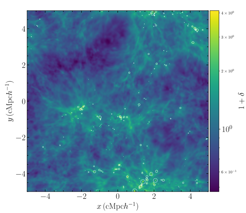
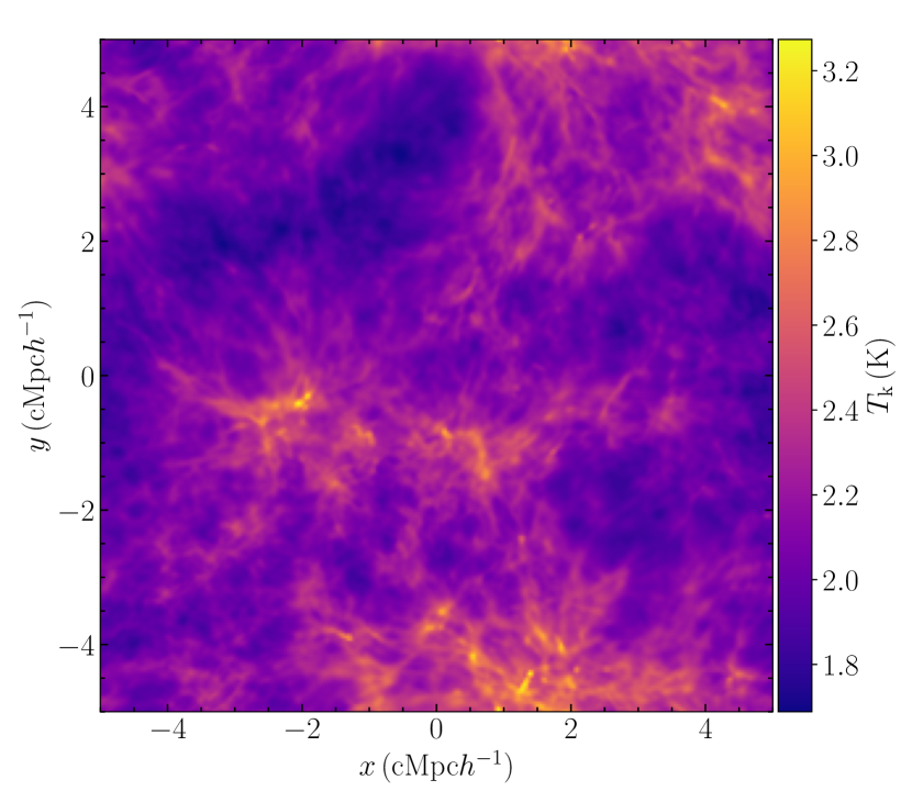
Figure 1: Left: projection-averaged gas overdensity, $1+\delta$ along the length in $\mathord{\mathchoice{\ooalign{$\displaystyle z$\cr\vrule height=2.05373pt,depth=-1.82124pt,width=2.29062pt\cr}\vphantom{\hbox{\set@color$\displaystyle z$}}}{\ooalign{$\textstyle z$\cr\vrule height=2.05373pt,depth=-1.82124pt,width=2.29062pt\cr}\vphantom{\hbox{\set@color$\textstyle z$}}}{\ooalign{$\scriptstyle z$\cr\vrule height=1.47249pt,depth=-1.24pt,width=1.60344pt\cr}\vphantom{\hbox{\set@color$\scriptstyle z$}}}{\ooalign{$\scriptscriptstyle z$\cr\vrule height=1.08498pt,depth=-0.8525pt,width=1.14531pt\cr}\vphantom{\hbox{\set@color$\scriptscriptstyle z$}}}}$ axis of our ramses simulation box. The white circles mark dark matter haloes, which serve as sources of UV photons in our subsequent RT computations. Circle size corresponds to the mass of the halo. Right: projection-averaged gas kinetic temperature $T_{\mathrm{k}}$ (K) along the length in $\mathord{\mathchoice{\ooalign{$\displaystyle z$\cr\vrule height=2.05373pt,depth=-1.82124pt,width=2.29062pt\cr}\vphantom{\hbox{\set@color$\displaystyle z$}}}{\ooalign{$\textstyle z$\cr\vrule height=2.05373pt,depth=-1.82124pt,width=2.29062pt\cr}\vphantom{\hbox{\set@color$\textstyle z$}}}{\ooalign{$\scriptstyle z$\cr\vrule height=1.47249pt,depth=-1.24pt,width=1.60344pt\cr}\vphantom{\hbox{\set@color$\scriptstyle z$}}}{\ooalign{$\scriptscriptstyle z$\cr\vrule height=1.08498pt,depth=-0.8525pt,width=1.14531pt\cr}\vphantom{\hbox{\set@color$\scriptscriptstyle z$}}}}$ axis of the simulation box. The box is a unigrid cube of length $10\,\mathrm{cMpc}h^{-1}$ on each side, with $256^{3}$ cells.

2.1 21-cm signal

Readers new to 21-cm physics are referred to more detailed accounts in reviews such as those by Furlanetto et al. (2006) and Pritchard & Loeb (2012); here we give only a brief summary. The 21-cm signal is a measurement of the 21-cm brightness against the CMB. In our previous papers (Mittal & Kulkarni, 2020; Mittal et al., 2022; Mittal & Kulkarni, 2022b) we worked with the ‘global’ signal, which is an average of the 21-cm brightness contrast over a cosmological volume. Here we work with a 21-cm signal at position r and redshift $z$, which is approximately given by

$$T_{21}(\textbf{{r}},z)=27x_{\text{H\,{i}}}(\textbf{{r}},z)\left[1+\delta(\textbf{{r}},z)\right]\left(\frac{1-Y_{\mathrm{p}}}{0.76}\right)\left(\frac{\Omega_{\mathrm{b}}h^{2}}{0.023}\right)\\ \times\sqrt{\frac{0.15}{\Omega_{\mathrm{m}}h^{2}}\frac{1+z}{10}}\left[1-\frac{T_{\gamma}(z)}{T_{\mathrm{s}}(\textbf{{r}},z)}\right]$\mathrm{mK}$\,,$$ (1)

where $T_{\mathrm{s}}$ is the spin temperature, $T_{\gamma}$ is the CMB temperature, $x_{\text{H\,{i}}}\equiv n_{\text{H\,{i}}}/(n_{\text{H\,{i}}}+n_{\text{H\,{ii}}})$ is the ratio of number densities of neutral hydrogen (H i) to the total hydrogen (H), and we have assumed a matter-dominated Universe so that $H(z)=H_{0}\sqrt{\Omega_{\mathrm{m}}(1+z)^{3}}$. The baryon overdensity is 1+$\delta(\textbf{{r}},z)=\rho_{\mathrm{b}}(\textbf{{r}},z)/\bar{\rho}_{\mathrm{b}}$, where $\bar{\rho}_{\mathrm{b}}$ is the mean of cosmic baryon density $\rho_{\mathrm{b}}(\textbf{{r}},z)$. As appropriate for high redshifts, such as in this work, we have ignored the gradient of peculiar velocity of gas cloud along the line of sight. In the presence of an excess radio background at frequencies $\sim$1.4\text{\,}\mathrm{GHz}$$ (Fixsen et al., 2011; Dowell & Taylor, 2018; Singal et al., 2023) one should replace CMB with CMB plus excess radio background (Feng & Holder, 2018; Fialkov & Barkana, 2019; Mittal & Kulkarni, 2022a). However, in this work we do not include the contribution of such a radio intensity.

We use the following expression for the spin temperature (which quantifies the relative population of hyperfine levels in a neutral hydrogen atom),

$$T_{\mathrm{s}}^{-1}(\textbf{{r}},z)\\ =\frac{x_{\gamma}(\textbf{{r}},z)T_{\gamma}^{-1}(z)+[x_{\mathrm{k}}(\textbf{{r}},z)+x_{\alpha}(\textbf{{r}},z)]T_{\mathrm{k}}^{-1}(\textbf{{r}},z)}{x_{\gamma}(\textbf{{r}},z)+x_{\mathrm{k}}(\textbf{{r}},z)+x_{\alpha}(\textbf{{r}},z)}\,,$$ (2)

where $T_{\mathrm{k}}$ is the gas temperature, $x_{\gamma}$, $x_{\mathrm{k}}$ and $x_{\alpha}$ are the 21-cm, collisional and Ly $\alpha$ coupling, respectively. Because of a near thermal equilibrium of gas and Ly $\alpha$ photons, we have made an assumption that the colour temperature is equal to the gas kinetic temperature, i.e., $T_{\alpha}\approx T_{\mathrm{k}}$ (Field, 1958). We do not discuss 21-cm and collisional coupling any further, and point the interested reader to the details in our previous work (Mittal et al., 2022).

Unlike in our previous work we have explicitly shown the position dependence on ionisation fraction, density and temperature (except for CMB, which is nearly uniform) in equation (2) to emphasise that we are interested in a non-global 21-cm signal. When we write $(\textbf{{r}},z)$ for any quantity (such as ionisation fraction, gas overdensity or gas temperature) derived from the simulated cosmological boxes, we mean the value of that field at the centre of cell located at r and redshift $z$ of the snapshot.

Besides the 21-cm signal itself we also look at its power spectrum. For 21-cm power spectrum we define the fluctuation in 21-cm signal as (in units of temperature)

$$\delta_{21}(\textbf{{r}})=T_{21}(\textbf{{r}})-\left\langle T_{21}\right\rangle\,,$$ (3)

where for brevity we dropped the $z$ dependence, and $\left\langle T_{21}\right\rangle$ represents the box or the space average of $T_{21}(\textbf{{r}})$. If the Fourier transform of $\delta_{21}(\textbf{{r}})$ is $\tilde{\delta}_{21}(\textbf{{k}})$ then the 21-cm power spectrum $P_{21}(k)$ is obtained via

$$\left\langle\tilde{\delta}_{21}(\bm{k_{1}})\tilde{\delta}_{21}(\bm{k_{2}})\right\rangle_{\mathrm{EA}}=(2\pi)^{3}\delta_{\mathrm{D}}(\bm{k_{1}}+\bm{k_{2}})P_{21}(\bm{k_{1}})\,,$$ (4)

where $\delta_{\mathrm{D}}$ is the Dirac-delta function and $\langle\cdot\rangle_{\mathrm{EA}}$ represents the ensemble average. We will quantify only the isotropic fluctuations so that we focus on the spherically averaged power spectrum in $k$ space, $P_{21}(\bm{k})=P_{21}(k)$. Also, instead of $P_{21}(k)$ we will illustrate our results in terms of

$$\Delta^{2}_{21}(k)=\frac{k^{3}}{2\pi^{2}}P_{21}(k)\,,$$ (5)

which has the dimensions of temperature-squared.

Gas density, temperature and neutral hydrogen fraction

We simulate the evolution and interaction of dark matter and gas via gravity, hydrodynamics and radiative cooling & heating using the cosmological adaptive mesh refinement (AMR) code ramses (Teyssier, 2002). In ramses DM particles are collisionless particles that interact only via gravity and to track their evolution a collisionless Boltzmann solver is used. The dynamics of gas on the other hand is modelled using the hydrodynamical Euler equations (in their conservative form) coupled to DM through gravity.

To get the number density of ionic species (only $n_{\text{H\,{i}}},n_{\text{H\,{ii}}}$ and $n_{\mathrm{e}}$ are of interest to us) we use the default ramses configuration where a collisional ionisation equilibrium – but not thermal equilibrium – is assumed. In this case, starting with a known primordial gas composition of hydrogen and helium, the number conservation along with the balance of creation and destruction rates uniquely determines all the abundances. The creation and destruction is governed by collisional ionisation and recombination, along with photoionisation if there is a non-zero ionising radiation present. Collisional ionisation, excitation, recombination and free-free emission (bremsstrahlung) inevitably give rise to a gas cooling collectively known as radiative cooling. Besides these channels there is also the inverse Compton cooling. Photoionisation heating is active only in the presence of a non-zero ionising radiation. Note that all of the above mentioned processes are effective and important at high densities and for gas temperatures above ${10}^{4}\text{\,}\mathrm{K}$ (Katz et al., 1996). As we neither investigate high density regions at small scales nor do we model reionisation where temperatures are high, radiative cooling is unimportant and the gas temperature falls adiabatically in accordance with the Hubble expansion. This translates to $T_{\mathrm{k}}\propto(1+z)^{2}$, assuming an ideal gas law for the baryonic gaseous matter of adiabatic index $\gamma=5/3$. In order to single out the effects of fully self-consistent 3D RT of Ly $\alpha$ photons we ignore X-ray heating or Ly $\alpha$ heating of IGM in this work. Impact of these processes is left for future analysis.

We get our initial conditions using first-order Lagrangian perturbation theory with Eisenstein & Hu (1998) fit to the CDM transfer function with baryonic features at $z=30$. We set our box size to $10\,\mathrm{cMpc}h^{-1}$ with $256^{3}$ cells, which implies each cell being $39\,\mathrm{ckpc}h^{-1}$ in size. We have a total of $256^{3}$ DM particles each of mass $4.55\times 10^{6}\,\mathrm{M}_{\odot}h^{-1}$. As we are not interested in simulations of individual stars/galaxies or structure formation we have worked on a uni-grid system, so that there is no grid refinement, for all the results of this work. After preparing initial conditions we run our hydrodynamic simulation down to $z\approx 9$. Maps of gas overdensity and temperature are shown in Fig. 1. We show a projected average of the quantity of interest which can be defined as

$$\tilde{f}(x,y)=\frac{\int f(x,y,\mathord{\mathchoice{\ooalign{$\displaystyle z$\cr\vrule height=2.28192pt,depth=-2.02362pt,width=2.54515pt\cr}\vphantom{\hbox{\set@color$\displaystyle z$}}}{\ooalign{$\textstyle z$\cr\vrule height=2.28192pt,depth=-2.02362pt,width=2.54515pt\cr}\vphantom{\hbox{\set@color$\textstyle z$}}}{\ooalign{$\scriptstyle z$\cr\vrule height=1.6361pt,depth=-1.37779pt,width=1.7816pt\cr}\vphantom{\hbox{\set@color$\scriptstyle z$}}}{\ooalign{$\scriptscriptstyle z$\cr\vrule height=1.20554pt,depth=-0.94724pt,width=1.27257pt\cr}\vphantom{\hbox{\set@color$\scriptscriptstyle z$}}}})\mathrm{d}\mathord{\mathchoice{\ooalign{$\displaystyle z$\cr\vrule height=2.28192pt,depth=-2.02362pt,width=2.54515pt\cr}\vphantom{\hbox{\set@color$\displaystyle z$}}}{\ooalign{$\textstyle z$\cr\vrule height=2.28192pt,depth=-2.02362pt,width=2.54515pt\cr}\vphantom{\hbox{\set@color$\textstyle z$}}}{\ooalign{$\scriptstyle z$\cr\vrule height=1.6361pt,depth=-1.37779pt,width=1.7816pt\cr}\vphantom{\hbox{\set@color$\scriptstyle z$}}}{\ooalign{$\scriptscriptstyle z$\cr\vrule height=1.20554pt,depth=-0.94724pt,width=1.27257pt\cr}\vphantom{\hbox{\set@color$\scriptscriptstyle z$}}}}}{\int\mathrm{d}\mathord{\mathchoice{\ooalign{$\displaystyle z$\cr\vrule height=2.28192pt,depth=-2.02362pt,width=2.54515pt\cr}\vphantom{\hbox{\set@color$\displaystyle z$}}}{\ooalign{$\textstyle z$\cr\vrule height=2.28192pt,depth=-2.02362pt,width=2.54515pt\cr}\vphantom{\hbox{\set@color$\textstyle z$}}}{\ooalign{$\scriptstyle z$\cr\vrule height=1.6361pt,depth=-1.37779pt,width=1.7816pt\cr}\vphantom{\hbox{\set@color$\scriptstyle z$}}}{\ooalign{$\scriptscriptstyle z$\cr\vrule height=1.20554pt,depth=-0.94724pt,width=1.27257pt\cr}\vphantom{\hbox{\set@color$\scriptscriptstyle z$}}}}}\,,$$ (6)

if projection is done along the $\mathord{\mathchoice{\ooalign{$\displaystyle z$\cr\vrule height=2.28192pt,depth=-2.02362pt,width=2.54515pt\cr}\vphantom{\hbox{\set@color$\displaystyle z$}}}{\ooalign{$\textstyle z$\cr\vrule height=2.28192pt,depth=-2.02362pt,width=2.54515pt\cr}\vphantom{\hbox{\set@color$\textstyle z$}}}{\ooalign{$\scriptstyle z$\cr\vrule height=1.6361pt,depth=-1.37779pt,width=1.7816pt\cr}\vphantom{\hbox{\set@color$\scriptstyle z$}}}{\ooalign{$\scriptscriptstyle z$\cr\vrule height=1.20554pt,depth=-0.94724pt,width=1.27257pt\cr}\vphantom{\hbox{\set@color$\scriptscriptstyle z$}}}}$ axis. The left panel shows the gas overdensity, $1+\delta$, the colour bar for which is in logarithmic scale. The white circles mark the DM haloes, found using HOP algorithm. The dark matter haloes will serve as sources of photons in our work (more on this in section 2.2). The average, maximum and minimum overdensity for this box are approximately $0.92,360$ and $0.02$, respectively. The right panel shows the gas kinetic temperature, $T_{\mathrm{k}}$, the colour bar for which is in linear scale. The average, maximum and minimum temperature for this box are approximately $2.13,86.5$ and $0.5\text{\,}\mathrm{K}$, respectively. Note that the mean value is consistent with the value expected from adiabatic evolution, i.e. $0.02(1+z)^{2}$ at $z\approx 9$ gives $2\text{\,}\mathrm{K}$. To read the ramses output we use the python package yt (Turk et al., 2010).

In our work the DM haloes will serve as our sources for photons (more on this later). For small box sizes, such as in this work, one may not find many collapsed objects at high redshifts. For this reason we do our analysis at a low redshift of $z\approx 9$ for simulations. While in reality cosmic dawn is expected to be at higher redshifts, our set-up is sufficiently useful in model building and for drawing useful conclusions.

Ly $\alpha$ coupling

We now discuss the Ly $\alpha$ coupling, $x_{\alpha}$. The probability that scattering of Ly $\alpha$ photon off a neutral hydrogen atom will cause a hyperfine transition is $4/27$ (Meiksin, 2000; Hirata, 2006; Dijkstra & Loeb, 2008a). If the rate of scattering of Ly $\alpha$ photons per atom is $P_{\alpha}$ then the Ly $\alpha$ coupling term is (Furlanetto et al., 2006)

$$x_{\alpha}=\frac{T_{*}}{T_{\gamma}}\frac{4P_{\alpha}}{27A_{10}}\,,$$ (7)

where $T_{*}=$0.068\text{\,}\mathrm{K}$$ and $A_{10}=$2.85\text{\times}{10}^{-15}\text{\,}\mathrm{Hz}$$ is the Einstein coefficient of spontaneous emission for the hyperfine transition. The scattering rate per atom may be calculated as

$$P_{\alpha}(\bm{r})=4\pi\int_{0}^{\infty}J(\bm{r},\nu)\sigma_{12}(\nu)\mathrm{d}\nu\,,$$ (8)

where $J$ and $\sigma_{12}$ are the local specific intensity (by number) and the cross-section of Ly $\alpha$ photons of frequency $\nu$, respectively. Discussion of its numerical computation is left for section 2.3.3.

2.2 The sources of Lyman-series photons

This section gives the description of the sources and the luminosity $L$ of our Lyman-series photons. The fundamental idea is that Lyman-series photons are produced by star forming galaxies that started appearing at cosmic dawn. Given the spectral energy distribution (SED) of the star/galaxy and an assumption that the emission rate should roughly follow the star formation rate we can construct the local emissivity function. We used a similar idea in our previous work to compute the uniform and homogeneous version of emissivity (Mittal & Kulkarni, 2020; Mittal et al., 2022). Our first ingredient required is the star formation rate density (SFRD) which is discussed next.

Given that we extract density or temperature from hydrodynamical simulation it would be logical to get SFRD from the simulation itself with a given star formation prescription. However, as we are working at redshifts of cosmic dawn, finding stars self-consistently is expensive as it can require not only large simulation boxes but high resolution as well. To circumvent this problem we construct our SFRD ‘by hand’ based on the idea of baryons collapsing into DM haloes turning into star particles. For this we would still need to locate the DM haloes, but this is readily done using a halo finder. Once these DM haloes are located (as shown in the left panel of Fig. 1 by white circles), we assume that each one of them contributes equally to the SFR of the full box. Following a simple analytical prescription for the SFRD (Furlanetto, 2006), the SFR due to each halo is

$$\mathrm{SFR_{per\ halo}}=\frac{V_{\mathrm{box}}}{N_{\mathrm{haloes}}}\times f_{\star}\bar{\rho}_{\mathrm{b}}\frac{\mathrm{d}F_{\mathrm{coll}}(z)}{\mathrm{d}t}\,,$$ (9)

where $f_{\star}$ is the star formation efficiency, $\bar{\rho}_{\mathrm{b}}$ is the mean cosmic baryon density today, $V_{\mathrm{box}}$ is the comoving box volume and $N_{\mathrm{haloes}}$ is the number of haloes found at the current snapshot.

We use a halo finder inspired by the HOP algorithm (Eisenstein & Hut, 1998) using the default value of density threshold, $\delta_{\mathrm{peak}}=160$. For the snapshot shown in Fig. 1, we find the minimum and maximum halo masses $1.96\times 10^{8}\,\mathrm{M}_{\odot}h^{-1}$ and $1.09\times 10^{10}\,\mathrm{M}_{\odot}h^{-1}$, respectively and a total of 213 haloes.

The star formation efficiency is a measure of the fraction of baryons that collapsed into the haloes and converted into star particles. In this work we take it to be $f_{\star}=0.1$ throughout. The fraction of DM that has collapsed into haloes is

$$F_{\mathrm{coll}}(z)=\mathrm{erfc}\left[\frac{\delta_{\mathrm{crit}}(z)}{\sqrt{2}\sigma(m_{\mathrm{min}})}\right]\,,$$ (10)

where $\delta_{\mathrm{crit}}$ is the linear critical overdensity of collapse and $\sigma^{2}$ is the variance in smoothed density field. The minimum halo mass for star formation is (Barkana & Loeb, 2001)

$$m_{\mathrm{min}}=\frac{10^{8}\mathrm{M}_{\odot}}{\sqrt{\Omega_{\mathrm{m}}h^{2}}}\left[\frac{10}{1+z}\frac{0.6}{\mu}\frac{\mathrm{min}(T_{\text{vir}})}{$1.98\text{\times}{10}^{4}$}\right]^{3/2}\,.$$ (11)

For atomic cooling threshold min($T_{\text{vir}})=${10}^{4}\text{\,}\mathrm{K}$$ and a fairly neutral medium at cosmic dawn $\mu\approx 1.22$. We do not include any feedback effects, such as the Lyman–Werner feedback.

If there are $N_{\mathrm{haloes}}^{i}$ haloes in a cell $i$ (cell location $\bm{r}_{i}$), then the local SFRD at $\bm{r}_{i}$ is

$$\dot{\rho_{\star}}(\bm{r}_{i},z)=N_{\mathrm{haloes}}^{i}\times\frac{\mathrm{SFR_{per\ halo}}}{V_{\mathrm{cell}}}\,.$$ (12)

where $V_{\mathrm{cell}}$ is the comoving volume of the $i^{\mathrm{th}}$ cell. With the above procedure we are finally able to obtain our SFRD in each cell and hence the local SFRD function, $\dot{\rho_{\star}}=\dot{\rho_{\star}}(\bm{r},z)$.

Next we need the SED of Lyman-series photons emitted from the stars and galaxies. Our knowledge of properties of stars and star formation at cosmic dawn is only speculative. Stellar population synthesis data of, such as BPASS or Bruzual & Charlot (2003), are calibrated to low redshift observations only. Thus, the employment of such data to high redshift is as good as any other model. We set SED of emission from any of these sources, residing in haloes, to be the same i.e. independent of halo mass, metallicity or age. Ly $\alpha$ photons can be generated in two ways: either the photons emitted by the source between Ly $\alpha$ and Ly $\beta$ frequencies get redshifted to Ly $\alpha$ photons, which we know as continuum photons, or via radiative cascading of higher Lyman-series photons, which are known as injected photons (Chen & Miralda-Escudé, 2004). In this work we do not account for the injected photons, i.e. our sources do not emit any photons beyond Ly $\beta$. Our SED – $\phi(\nu)$, defined in terms of number of photons per baryonic particle per unit frequency range – follows a Pop-II model so that it is proportional to $\nu^{-0.86}$ extending from Ly $\alpha$ to Ly $\beta$ frequencies with the normalisation set to $N_{\alpha\beta}=6520$ photons per baryonic particle (Barkana & Loeb, 2005). As pointed out by Chuzhoy & Zheng (2007, hereafter CZ07) owing to the short range of continuum photons the results should only be mildly dependent on our SED choice. Note that for simplicity we assume that the DM haloes are at rest so that the frequency of photons emitted in their rest frame is same as in the global frame. Also, we assume an isotropic emission from each halo.

Finally, with the SED and SFRD in place, the local emissivity (in terms of number of photons per unit comoving volume per unit time per unit frequency) at redshift $z$ and frequency $\nu$ is

$$\epsilon(\bm{r},\nu,z)=\frac{1}{m_{\mathrm{b}}}\dot{\rho}_{\star}(\bm{r},z)\phi(\nu)\,,$$ (13)

where $m_{\mathrm{b}}\approx 1.22m_{\mathrm{H}}$ is the average baryon mass and $m_{\mathrm{H}}$ being the hydrogen mass. Consequently, the total luminosity (required for equation 28) in a box of comoving volume $V_{\mathrm{box}}$ can be written as

$$L=V_{\mathrm{box}}N_{\alpha\beta}f_{\star}\bar{n}_{\mathrm{b}}\frac{\mathrm{d}F_{\mathrm{coll}}(z)}{\mathrm{d}t}\,,$$ (14)

where $\bar{n}_{\mathrm{b}}$ is the global average baryon comoving number density. As an example at $z\sim 9$ and for a box of side length $10\,\mathrm{cMpc}h^{-1}$ we have $L=$8.91\text{\times}{10}^{55}\text{\,}\mathrm{s}^{-1}$$.

2.3 Radiative transfer of Ly $\alpha$ photons

We use rascas (Michel-Dansac et al., 2020) to post-process our ramses simulation (thus accounting for cosmological density, temperature and bulk motion) to do a propagation of Ly $\alpha$ photons with multiple scatterings. We use the version presented by Garel et al. (2021) that includes an implementation of the Hubble flow, but we make three main modifications described in sections 2.3.1, 2.3.2 and 2.3.3, respectively – (i) the introduction of a global comoving frame in which photons redshift during their propagation, (ii) stopping criterion for photon propagation, and (iii) the computation of the scattering rate per atom.

We give here a general description of the algorithm of Monte Carlo radiative transfer (MCRT) of Ly $\alpha$ photons. Readers familiar with the RT details may skip and jump straight to the results section below. Before we get to the more detailed version of MCRT algorithm we describe three types of reference frames of interest. These are as follows:

• Global comoving frame: an observer in this frame can see both contributions to the velocity, viz., macroscopic bulk or peculiar velocity $(\textbf{{v}}_{\mathrm{b}})$ and microscopic thermal motion $(\textbf{{v}}_{\mathrm{th}})$ of the hydrogen atom. One can think of this observer to be sitting at the corner of the cosmological box observing all the events happening. We put no subscript on the photon’s frequency in this frame.

• Cell or gas frame: an observer in this frame cannot see the bulk velocity of gas but only the thermal velocity. It is in this frame that the line profile of atomic transition is a Voigt function. We use the subscript ‘cell’ on $\nu$ to represent the frequency of photons in this frame. Thus,

  $$\nu_{\mathrm{cell}}=\nu\left(1-\frac{\textbf{{v}}_{\mathrm{b}}}{c}\cdot\hat{\textbf{{k}}}\right)\,,$$ (15)

  where $\hat{\textbf{{k}}}$ is the photon’s direction of propagation. In the above equation – and for similar ones that follow – we used the linearised version of the Lorentz transformation as appropriate for non-relativistic velocities.

• Atom frame: as the name suggests, the observer does not see any velocity and the atom is at rest. The line profile in this frame is simply the natural (Lorentzian) line profile. We use the subscript ‘atom’ on $\nu$ to represent the frequency in this frame. Thus,

  $$\nu_{\mathrm{atom}}=\nu_{\mathrm{cell}}\left(1-\frac{\textbf{{v}}_{\mathrm{th}}}{c}\cdot\hat{\textbf{{k}}}\right)=\nu\left(1-\frac{\textbf{{v}}_{\mathrm{b}}+\textbf{{v}}_{\mathrm{th}}}{c}\cdot\hat{\textbf{{k}}}\right)\,,$$ (16)

  where we neglected the second-order term in velocity.

We now discuss the main steps in MCRT describing the important concepts along the way.

1. Initialising the photon: a photon is started from the source of known position. We assign it a direction $(\hat{\textbf{{k}}})$ chosen from an isotropic distribution and a frequency (in the source frame) chosen from a given SED of the source i.e. spectral sampling from the SED (Michel-Dansac et al., 2020). Then we translate the frequency to external frame according to the source velocity. Note that in our work the sources (DM haloes) are at rest in which case frequency in source and external frame are the same.

2. Propagating the photon: after emission (or a scattering event) we assign the photon a new optical depth, which we choose from an exponential distribution, i.e., $\tau_{\mathrm{event}}=-\ln(1-r)$, for a random number $r\in[0,1)$. We then move the photon a real physical distance along its current direction of propagation such that the optical depth it covers is $\tau_{\mathrm{event}}$. At the new location, a resonant scattering occurs.

   Michel-Dansac et al. (2020) move the photons from event to event depending on the ambient density, temperature, and the photon frequency until the optical depth accumulates to $\tau_{\mathrm{event}}$. By an ‘event’ we mean either a cell-crossing event or a scattering event. For a distance $l$ inside a cell of number density $n_{\text{H\,{i}}}$ and gas temperature $T_{\mathrm{k}}$ the optical depth for the Ly $\alpha$ photon is

   $$\tau=n_{\text{H\,{i}}}\sigma_{12}(\nu,T_{\mathrm{k}})l\,.$$ (17)

   In the above we assumed that all hydrogen atoms are in the ground state, so that $n_{\text{H\,{i}},1}\approx n_{\text{H\,{i}}}$, because of the smallness of transition time ($A_{21}^{-1}\sim${10}^{-9}\text{\,}\mathrm{s}$$) compared to other times scales and the high characteristic temperature for $1\to 2$ excitation compared to $T_{\mathrm{k}}$. Note that we do not assume any deuterium or dust impurities in the IGM gas in any of the models in our work.

   The photon propagation picture presented above is applicable to a non-Hubble-expanding system. With Hubble flow in action the optical depth calculation needs modification and is discussed in section 2.3.1.

   Independent of Hubble flow or not, in MCRT codes one finds it easiest to work in gas/cell frame when computing the optical depth in which case the cross-section is represented by the convolution of natural (Lorentzian) and thermal (Gaussian) line profiles. Thus,

   $$\sigma_{\mathrm{V}}(\nu_{\mathrm{cell}},T_{\mathrm{k}})=\frac{3\lambda_{\alpha}^{2}a}{2\sqrt{\pi}}H_{a}(x_{\mathrm{cell}})\,,$$ (18)

   where $x_{\mathrm{cell}}=(\nu_{\mathrm{cell}}-\nu_{\alpha})/\Delta\nu_{\mathrm{D}}$ and $a=A_{21}/(4\pi\Delta\nu_{\mathrm{D}})$ is the ratio of natural to thermal line broadening for $A_{21}=$6.25\text{\times}{10}^{8}\text{\,}\mathrm{Hz}$$, the Einstein spontaneous emission coefficient of Ly $\alpha$ transition. The line centre frequency for Ly $\alpha$ is $\nu_{\alpha}=$2.47\text{\times}{10}^{15}\text{\,}\mathrm{Hz}$$. The Voigt function is defined as

   $$H_{a}(x)=\frac{a}{\pi}\int_{-\infty}^{\infty}\frac{\mathrm{e}^{-y^{2}}}{(x-y)^{2}+a^{2}}\mathrm{d}y\,,$$ (19)

   which is a non-dimensional function normalised such that $\int H_{a}(x)\mathrm{d}x=\sqrt{\pi}$. The temperature dependence enters through the Doppler width $\Delta\nu_{\mathrm{D}}=b/\lambda_{\alpha}$, where $b=(2k_{\mathrm{B}}T_{\mathrm{k}}/m_{\mathrm{H}})^{1/2}$ is the mean thermal velocity for hydrogen atom of mass $m_{\mathrm{H}}$ and $\lambda_{\alpha}=$1215.67\text{\,}\mathrm{\SIUnitSymbolAngstrom}$$ is the central wavelength.

3. Scattering: after we have moved the photon by a physical distance governed by $\tau_{\mathrm{event}}$ a scattering event occurs where we assign the photon a new direction and frequency. The angle by which the photon is scattered is decided by the phase function. If $\mu=\cos\theta$, where $\theta$ is the scattering angle or the angle between the outgoing and incoming direction of the photon, then the probability of $\cos\theta$ to be in $\mu$ to $\mu+\mathrm{d}\mu$ is $\mathcal{P}(\mu)\mathrm{d}\mu$. For the Ly $\alpha$ line, there are two limiting cases depending on whether the photon is in the core or wings of the line profile as seen by the atom just before scattering (Dijkstra & Loeb, 2008b),

   $$\mathcal{P}(\mu)=\begin{cases}(11+3\mu^{2})/24,\text{ if }|\nu_{\mathrm{atom,in}}-\nu_{\alpha}|<0.2\Delta\nu_{\mathrm{D}}\\ 3(1+\mu^{2})/8,\text{ otherwise}\,,\end{cases}$$ (20)

   and $\mu$ goes from $-1$ to 1. For simplicity, we label this as anisotropic scattering. Note that under the assumption of non-relativistic velocities the angle of scattering $\theta$ is the same in any frame.

   Without the loss of generality, let us align the incoming photon along the positive $x$ axis and the outgoing photon in $xy$ plane, so that $\hat{\textbf{{k}}}_{\mathrm{in}}=(1,0,0)$ and $\hat{\textbf{{k}}}_{\mathrm{out}}=(\mu,\sqrt{1-\mu^{2}},0)$. In this coordinate system only the $x$ component (parallel) and $y$ component (perpendicular) of thermal velocity are important for the determination of $\hat{\textbf{{k}}}_{\mathrm{out}}$.

   We choose the parallel velocity component from a Maxwell–Boltzmann distribution biased by the fact that it is such that the photon appears closer to resonance. Thus, the probability distribution of parallel thermal velocity component is

   $$P_{\parallel}(u^{\parallel}_{\mathrm{th}})=\frac{1}{H_{a}(x_{\mathrm{cell,in}})}\frac{a}{\pi}\frac{\mathrm{e}^{-{u^{\parallel}_{\mathrm{th}}}^{2}}}{\left(x_{\mathrm{cell,in}}-u^{\parallel}_{\mathrm{th}}\right)^{2}+a^{2}}\,,$$ (21)

   where $u^{\parallel}_{\mathrm{th}}=v^{\parallel}_{\mathrm{th}}/b$ is the non-dimensionalised parallel component of thermal velocity. The perpendicular component, on the other hand, is not seen by the photon and hence we choose it from a pure 1D Maxwell–Boltzmann distribution, which is simply a Gaussian function. Thus,

   $$P_{\perp}(u^{\perp}_{\mathrm{th}})=\frac{1}{\sqrt{\pi}}\mathrm{e}^{-{u^{\perp}_{\mathrm{th}}}^{2}}\,.$$ (22)

   Having obtained $\mu$ (and hence $\hat{\textbf{{k}}}_{\mathrm{out}}$) and $\textbf{{v}}_{\mathrm{th}}=(bu^{\parallel}_{\mathrm{th}},bu^{\perp}_{\mathrm{th}},\text{`not important'})$ the new frequency to first order in $\textbf{{v}}_{\mathrm{th}}/c$ is

   $$\nu_{\mathrm{cell,out}}=\nu_{\mathrm{cell,in}}\frac{1+(\hat{\textbf{{k}}}_{\mathrm{out}}-\hat{\textbf{{k}}}_{\mathrm{in}})\cdot\textbf{{v}}_{\mathrm{th}}/c}{1+(1-\hat{\textbf{{k}}}_{\mathrm{out}}\cdot\hat{\textbf{{k}}}_{\mathrm{in}})h_{\mathrm{P}}\nu_{\mathrm{cell,in}}/m_{\mathrm{H}}c^{2}}\,,$$ (23)

   where $h_{\mathrm{P}}$ is the Planck’s constant. Numerator is just the term due to a change of frames assuming a coherent scattering in atom frame, i.e., $\nu_{\mathrm{atom,in}}=\nu_{\mathrm{atom,out}}$. But if recoil in the atom is taken into account then there is a partial transfer of energy from photon to atom, which means the outgoing frequency is slightly lowered by the factor in the denominator (Adams, 1972; Zheng & Miralda-Escudé, 2002). Figure 9 illustrates the effect of recoil on the output specific intensity in an idealised configuration.

4. Stopping criterion: we repeat steps 2 and 3 until the IGM becomes transparent enough for the photon. See section 2.3.2 for details on this.

We repeat all steps for a desired number of Monte Carlo (MC) photons to achieve convergence.

Some general remarks about our RT approach are in order. rascas is a passive RT code i.e. RT does not have any effect on the hydrodynamics or in other words the gas density and temperature distribution provided by ramses serve as a fixed background on which RT is run.

Related to the above point, note that when we write ‘recoil in the atom’ it is mentioned here only as a theoretical concept meant to explain the decrease in photon energy. In actual computation in the code, the energy transfer is a one-sided process which affects only the photon since rascas is a passive RT code run in post-process. If indeed the energy gain in the atom is taken into account then it gives rise to the so-called ‘Ly $\alpha$ heating’. However, this heating is quite small and we do not expect the energy conservation violation to be severe. One can realise the smallness of the recoil effect by comparing the energy of a Ly $\alpha$ photon and the rest mass energy of a hydrogen atom, i.e., $h_{\mathrm{P}}\nu_{\alpha}/m_{\mathrm{H}}c^{2}\sim 10^{-8}$.

A final important point we mention is that our purpose of RT simulation is not to calculate the Ly $\alpha$ spectrum escaping some domain but rather the rate of scattering, $P_{\alpha}$, over the full domain volume.

Figure 2: This schematic demonstrates our calculation of the rate of scattering per atom, $P_{\alpha}$. Shown are trajectories of two example photons in cells $c_{1}$ and $c_{2}$ from our cosmological box. Red and blue dots mark scattering and cell-crossing events, respectively. Both photons originate from location ‘0’. (Although this schematic is shown for 2D, it is easy to visualise the concept in 3D.)

2.3.1 Hubble flow

Michel-Dansac et al. (2020) did not account for redshifting of photons. Often in MCRT codes one works in global rest frame to capture the effect of Hubble expansion. In this case scatterers are given an additional Hubble flow velocity keeping the frequency of the photon unchanged as it freely propagates between scatterings. This is a reasonable approach as long as the mean free path of the photons is small. We instead work in a comoving frame when the photon is in free propagation. In such a case the observer does not see any additional Hubble flow velocity of atoms but directly redshifts the photons as they propagate.

With redshifting in place an additional complication arises in either of the approaches mentioned above: redshifting the photons corresponding to a large distance $l$ in just one step may cause large shifts in $x_{\mathrm{cell}}$ even though $\nu$ may change by a very small amount. This may cause the photon to miss the essential core scatterings where the line profile is sharply peaked. Hence, following Garel et al. (2021), we use an adaptive scheme to accurately account for the H i-Ly $\alpha$ overlap. In this method, instead of moving photons over large steps of length $l$ we move them over sub-cell lengths, $\delta l$. For sufficiently small $\delta l$ one correctly captures the redshifting by altering the frequency by a factor of $(1-H\delta l/c)$ as well as does not miss the essential core scatterings.

Consider a photon at redshift $z_{0}$ of frequency $\nu_{0}$ at some location and after a short time interval $\delta t$ it reaches $z_{1}$ at frequency $\nu_{1}$. In a Hubble expanding medium, the frequencies can be related as

$$\frac{\nu_{1}}{1+z_{1}}=\frac{\nu_{0}}{1+z_{0}}\,.$$ (24)

For a small distance travelled by the photon, $\delta l$, the change in redshift is $z_{1}-z_{0}=\delta z$, where $|\delta z|\ll 1$. We get

$$\nu_{1}=\nu_{0}\left(1+\frac{\delta z}{1+z_{0}}\right)\,.$$ (25)

Eliminating $z$’s using the definition of Hubble factor and writing in terms of $\delta t$, we get $\nu_{1}=\nu_{0}(1-H\delta t)$. Finally, setting $\delta t=\delta l/c$ the above becomes

$$\nu_{1}=\nu_{0}\left(1-\frac{H\delta l}{c}\right)\,.$$ (26)

The assumption made in the above derivation is that the Hubble factor does not change significantly for a photon propagating in a fixed snapshot. This condition is satisfied for small distances $\delta l$ and a small overall distance covered on its journey.

With this new scheme of propagation equation (17) is modified to

$$\tau=\sum_{i}n_{\text{H\,{i}}}\sigma_{\mathrm{V}}(\nu_{i},T_{\mathrm{k}})\delta l_{i}\,,$$ (27)

where $\nu_{i+1}$ is related to previous frequency $\nu_{i}$ via equation (26).

For a quantitative comparison of the two implementations – first in which the gas atoms are given Hubble flow velocity and the second in which we directly reduce the photon frequency – see section A.2.

2.3.2 IGM transparency

As we use periodic boundary conditions for the photons, we give details of the stopping criterion of our MCRT procedure. We terminate the MCRT in step 4 when the IGM becomes transparent enough or in other words when the photon has drifted far to the red wings of the line profile. Quantitatively we set the stopping criterion to be when the cell frame frequency, $\nu_{\mathrm{cell}}$, goes below $(\nu_{\alpha}-6\Delta\nu_{\mathrm{D}})$, i.e. when $x_{\mathrm{cell}}\leqslant-6$. In such a case the cross-section at the critical frequency relative to that at the line centre is, for example, $\sigma_{\mathrm{V}}(\nu_{\mathrm{cell}},T_{\mathrm{k}})/\sigma_{\mathrm{V}}(\nu_{\alpha},T_{\mathrm{k}})\approx 8.1\times 10^{-4}$ and $7.8\times 10^{-5}$ at $T_{\mathrm{k}}=1$ and $100\text{\,}\mathrm{K}$, respectively. In configurations which require $T_{\mathrm{k}}=0$ we stop the MCRT when the cell frame frequency goes below $(\nu_{\alpha}-60\tilde{A})$, where $\tilde{A}=A_{21}/(4\pi)$. For this choice, $\sigma_{\mathrm{L}}(\nu_{\mathrm{cell}})/\sigma_{\mathrm{L}}(\nu_{\alpha})\approx 2.8\times 10^{-4}$, where $\sigma_{\mathrm{L}}$ is the Lorentzian cross-section.

2.3.3 Rate of Ly $\alpha$ scattering

In numerical simulations it can be computationally expensive to record $J(\bm{r},\nu)$ because it is a four dimensional quantity. It is thus simpler to work directly with $P_{\alpha}(\bm{r})$ in order to get $x_{\alpha}$. Following Lucy (1999) and Seon & Kim (2020), we compute $P_{\alpha}$ in a cell by summing optical depth segments due to all the MC photons that visited that cell times the luminosity (by number) carried by each MC photon normalised to the number of atoms in that cell. Thus, the scattering rate per atom in a cell ‘X’ is

$$P_{\alpha}(\mathrm{X})=\frac{L/N_{\mathrm{mc}}}{V_{\mathrm{X}}n_{\text{H\,{i}},\mathrm{X}}}\sum\tau_{\mathrm{X}}\,,$$ (28)

where $L$ is the total box luminosity by number (equation 14), $N_{\mathrm{mc}}$ is the number of MC photons used, $V_{\mathrm{X}}$ is the volume of cell X, $n_{\text{H\,{i}},\mathrm{X}}$ is the neutral hydrogen number density in cell X and $\sum\tau_{\mathrm{X}}$ is the total optical depth in cell X due to all the MC photons that crossed this cell. Note that a slightly more accurate approach to $P_{\alpha}$ is to count the number of scatterings rather than summing the optical depths in which case one must replace $\sum\tau_{\mathrm{X}}$ by $N_{\mathrm{scatt,X}}$, the number of scatterings in each cell (Seon & Kim, 2020). However, we work with the definition in equation (28) for reasons discussed in appendix B.

Figure 2 illustrates the scheme of equation (28) diagrammatically in a toy model consisting of 2 cells $c_{1}$ and $c_{2}$ and 2 MC photons. The cell crossings are marked by blue dots and scattering events are shown by red dots. In cell $c_{1}$ there are 2 segments of the photon trajectory namely $0\to 1$ and $0\to 5$. Accordingly the scattering rate following equation (28) will be

$$\frac{L/2}{V_{c_{1}}n_{\text{H\,{i}},c_{1}}}(\tau_{01}+\tau_{05})\,.$$

Similarly in cell $c_{2}$ there are 4 segments $1\to 2,2\to 3,3\to 4$ and $5\to 6$ and hence

$$\frac{L/2}{V_{c_{2}}n_{\text{H\,{i}},c_{2}}}(\tau_{12}+\tau_{23}+\tau_{34}+\tau_{56})\,,$$

where $\tau_{ij}$ refers to the optical depth corresponding to the length segment $l_{ij}$ and $i,j$ label the scattering or cell-crossing event.

In order to get a ‘converged’ $P_{\alpha}$, one requires a large number of MC photons for a given number of cells. For our main results in this work, we have used $N_{\mathrm{mc}}=10^{8}$ and $256^{3}$ cells in a cube of side length $10\,\mathrm{cMpc}h^{-1}$. The MC noise associated with our RT simulation is discussed in section 4.

2.4 Ly $\alpha$ coupling without multiple scatterings

In section 3, we intend to compare the method presented in this paper (accounting for multiple Ly $\alpha$ scatterings) with our previous work (Mittal & Kulkarni, 2020) which did not include this effect. Therefore, we briefly summarise the framework introduced in Mittal & Kulkarni (2020) modified to 3D calculation below.

We use the following expression for the Ly $\alpha$ coupling term

$$x_{\alpha}=(1-\delta_{\alpha})\frac{J_{\alpha}}{J_{0}}\,,$$ (29)

where

$$J_{0}\approx$5.54\text{\times}{10}^{-8}$(1+z)\,${\mathrm{m}}^{-2}\text{\,}{\mathrm{s}}^{-1}\text{\,}{\mathrm{Hz}}^{-1}\text{\,}{\mathrm{sr}}^{-1}$\,.$$ (30)

The distortion in the Ly $\alpha$ background due to interaction with neutral hydrogen atom under the wing approximation is quantified by $\delta_{\alpha}$. See Mittal & Kulkarni (2020) for more details.

In this formalism we need the background Ly $\alpha$ specific intensity, $J_{\alpha}(\bm{r},z)=J(\bm{r},z,\nu=\nu_{\alpha})$, throughout the simulation box. In our previous works we used the following equation (Mittal & Kulkarni, 2020)

$$J_{\alpha}(z)=\frac{c}{4\pi}(1+z)^{2}\int\frac{\epsilon(\nu^{\prime},z^{\prime})}{H(z^{\prime})}\,\mathrm{d}z^{\prime}\,,$$ (31)

for the computation of $J_{\alpha}$. However, the above is applicable only when we have a continuous uniform emission over the whole volume of interest; position information was irrelevant for the resulting $J_{\alpha}$. In our current system emission is not uniformly distributed over the volume. Instead emission occurs from specific sites (which in this work we set at the DM halo positions).

For 3D version of equation (31), we follow Santos et al. (2008, 2010) to get the spherically averaged number of photons arriving per unit proper area per unit proper time per unit frequency per unit solid angle,

$$J_{\alpha}(\bm{r},z)=\frac{1}{4\pi}(1+z)^{2}\int_{0}^{r_{\mathrm{max}}}\int\epsilon(\bm{r}+\bm{r}^{\prime},\nu^{\prime},z^{\prime})\,\frac{\mathrm{d}\Omega^{\prime}}{4\pi}\mathrm{d}r^{\prime}\,,$$ (32)

where

$$\nu^{\prime}=\nu_{\alpha}(1+z^{\prime})/(1+z)\,,$$ (33)

$z$ is the redshift of our snapshot and $z^{\prime}$ is the redshift at the source from where the photons start and reach the point of interest $(\bm{r},z)$ while travelling in a straight line a comoving distance of $r^{\prime}$. For a given $z$ and $r^{\prime}$, $z^{\prime}$ is obtained via

$$r^{\prime}=\int_{z}^{z^{\prime}}\frac{c}{H(z^{\prime\prime})}\mathrm{d}z^{\prime\prime}\,.$$ (34)

Note how $J_{\alpha}$ is independent of local gas density, local gas temperature and line profile shape – and hence any off-centre scatterings – since there is no scattering factor $\mathrm{e}^{-\tau}$ in the computation of equation (32). The assumption $\tau=0$ originates from the notion of employing a Dirac-delta cross-section centred at resonant frequency. In such a scenario bluer photons have no overlap with the scatterer allowing the photons to travel long distances without getting scattered at all. They are scattered only when they cosmologically redshift to line centre.

Because $J_{\alpha}$ is independent of local physical quantities, $x_{\alpha}$ is also independent of them (except weakly through $\delta_{\alpha}$, which is typically $\sim 0$). This formalism has been used in popular 21-cm codes such as 21cmFAST (Mesinger et al., 2011).

For consistency with the SED used in this work we have not added the contribution of higher Lyman-series photons to the total intensity in equation (32). The maximum comoving distance, away from the desired position a photon could have started so that it reaches at Ly $\alpha$ frequency, allowed is $r_{\mathrm{max}}$. It may be computed by setting $\nu^{\prime}$ to $\nu_{\beta}$ – which is the frequency of Ly $\beta$ line – in equation (33) and putting the corresponding $z^{\prime}$ into equation (34).

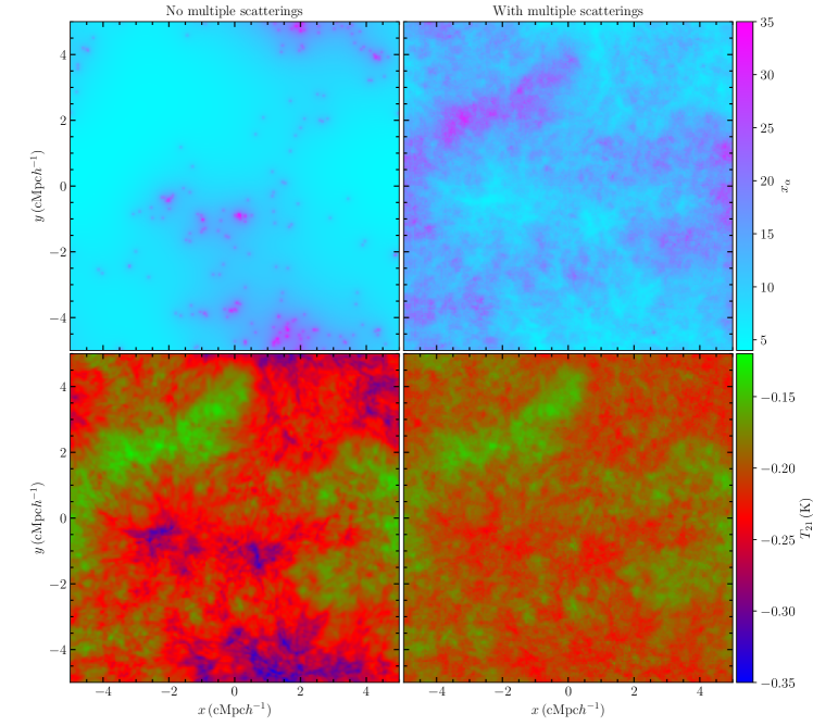
Figure 3: Top panels show projected average along the full depth in $\mathord{\mathchoice{\ooalign{$\displaystyle z$\cr\vrule height=2.05373pt,depth=-1.82124pt,width=2.29062pt\cr}\vphantom{\hbox{\set@color$\displaystyle z$}}}{\ooalign{$\textstyle z$\cr\vrule height=2.05373pt,depth=-1.82124pt,width=2.29062pt\cr}\vphantom{\hbox{\set@color$\textstyle z$}}}{\ooalign{$\scriptstyle z$\cr\vrule height=1.47249pt,depth=-1.24pt,width=1.60344pt\cr}\vphantom{\hbox{\set@color$\scriptstyle z$}}}{\ooalign{$\scriptscriptstyle z$\cr\vrule height=1.08498pt,depth=-0.8525pt,width=1.14531pt\cr}\vphantom{\hbox{\set@color$\scriptscriptstyle z$}}}}$ axis of the Ly $\alpha$ coupling $x_{\alpha}$, calculated without (left) and with (right) multiple scatterings. Bottom panels show the corresponding 21-cm signal $T_{21}$, projected average along the $\mathord{\mathchoice{\ooalign{$\displaystyle z$\cr\vrule height=2.05373pt,depth=-1.82124pt,width=2.29062pt\cr}\vphantom{\hbox{\set@color$\displaystyle z$}}}{\ooalign{$\textstyle z$\cr\vrule height=2.05373pt,depth=-1.82124pt,width=2.29062pt\cr}\vphantom{\hbox{\set@color$\textstyle z$}}}{\ooalign{$\scriptstyle z$\cr\vrule height=1.47249pt,depth=-1.24pt,width=1.60344pt\cr}\vphantom{\hbox{\set@color$\scriptstyle z$}}}{\ooalign{$\scriptscriptstyle z$\cr\vrule height=1.08498pt,depth=-0.8525pt,width=1.14531pt\cr}\vphantom{\hbox{\set@color$\scriptscriptstyle z$}}}}$ axis. The box-averaged value of the 21-cm signal for left- and right-hand sides are $\langle T_{21}\rangle=$-215.98\text{\,}\mathrm{mK}$$ and $-195.60\text{\,}\mathrm{mK}$, respectively. The box is of size $10\,\mathrm{cMpc}h^{-1}$ with $256^{3}$ cells.

Equation (32) maybe more useful when written in terms of a single volume integral, emissivity in terms of SED-SFRD and with replacement $\bm{r}+\bm{r}^{\prime}\to\bm{r}^{\prime}$. Thus,

$$J_{\alpha}(\bm{r},z)=\frac{1}{4\pi}(1+z)^{2}\frac{1}{m_{\mathrm{b}}}\int\left[\dot{\rho}_{\star}(\bm{r}^{\prime},z)\right]\left[\frac{\phi(\nu^{\prime})}{4\pi|\bm{r}-\bm{r}^{\prime}|^{2}}\right]\mathrm{d}^{3}r^{\prime}\,.$$ (35)

where $\nu^{\prime}=\nu^{\prime}(|\bm{r}-\bm{r}^{\prime}|)$. In the above relation we have made an assumption that the SFRD affects $J_{\alpha}$ instantaneously so that in the second argument of $\dot{\rho}_{\star}$ we set $z^{\prime}\approx z$.

Table 1: Simulations A to F designed to investigate the relative importance of different ingredients of Ly $\alpha$ radiative transfer. The bottom 5 rows list the values of $x_{\alpha}$ and $T_{21}$ in all simulations, and their difference from the fiducial simulation.

Process	A	B	C	D	E	F	Fiducial
Bulk motion	No	Yes	No	Yes	Yes	Yes	Yes
Cosmological H i density	No	No	Yes	No	Yes	Yes	Yes
Non-zero temperature	No	No	Yes	Yes	Yes	Yes	Yes
Anisotropic scattering	No	No	Yes	Yes	Yes	No	Yes
Recoil	No	No	Yes	Yes	No	Yes	Yes
Results
Mean difference from fiducial in $x_{\alpha}$	$-10.6$	$-12.5$	$1.9$	$-5.8$	$2.4$	$-0.1$	0
RMS difference from fiducial in $x_{\alpha}$	$17.7$	$18.8$	$14.3$	$15.8$	$10.8$	$13.2$	0
Box-averaged $T_{21}\,$(mK)	$-166.62$	$-78.74$	$-213.06$	$-195.86$	$-199.78$	$-195.43$	$-195.60$
Mean difference from fiducial in $|T_{21}|\,$(mK)	$-29.0$	$-116.9$	$17.5$	$0.3$	$4.2$	$-0.2$	0
RMS difference from fiducial in $|T_{21}|\,$(mK)	$77.7$	$132.5$	$71.6$	$68.8$	$44.8$	$61.6$	0

The fact that the integral in equation (35) is a convolution of two functions, viz., $\dot{\rho}_{\star}$ and $\phi/4\pi r^{2}$, saves us a lot of time computationally. Since a direct computation of the integral can be expensive, one may resort to convolution theorem of Fourier transforms.

3 Results

Figure 3 shows our main result: the Ly $\alpha$ coupling (top panels) and the corresponding 21-cm signal (bottom panels). The left panels show the quantities without multiple scatterings (using the scheme in section 2.4) and the right panels show them with multiple scatterings (using our RT simulation set-up described in section 2.3).

Comparing the Ly $\alpha$ coupling maps visually one can immediately notice the differences. In the case without multiple scatterings, the photons have a vanishing cross-section away from the centre. Consequently, they have the freedom to travel large distances without getting scattered. So the photons travel in straight lines and can get scattered only when they reach the line centre beyond which they do not make any impact. In this case the gas density and temperature inhomogeneities are not reflected $x_{\alpha}$ and consequently $x_{\alpha}$ has a smooth distribution away from the sources. On the other hand when there is a finite spread in the cross-section around the line centre photons undergo scatterings not only on the blue side but on the red side as well and continue to do so until the medium becomes transparent. As a consequence $x_{\alpha}$ picks up the density and temperature inhomogeneities as well as exhibits a non-spherical symmetry around the sources.

The mean and root mean square (RMS) difference in $x_{\alpha}$ between the computation with multiple scatterings and that without is $\langle\Delta x_{\alpha}\rangle=-4.8$ and $\sqrt{\langle(\Delta x_{\alpha})^{2}\rangle}=17.8$, respectively. ($\Delta x_{\alpha}$ represents $x_{\alpha,\mathrm{No\ MS}}-x_{\alpha,\mathrm{MS}}$). Similarly, mean and RMS of the difference in 21-cm signal magnitude are $\langle\Delta|T_{21}|\rangle=$20.4\text{\,}\mathrm{mK}$$ and $\sqrt{\langle(\Delta|T_{21}|)^{2}\rangle}=$82.8\text{\,}\mathrm{mK}$$, respectively. The box-averaged 21-cm signal is $-215.98\text{\,}\mathrm{mK}$ without multiple scatterings and $-195.60\text{\,}\mathrm{mK}$ with multiple scatterings. Consequently, the relative difference (RMS) in terms of 21-cm signal between with and without multiple scatterings is 42.3 %. We conclude that accounting for multiple scatterings can have a significant impact on the 21-cm signal. Multiple scatterings also have a substantial impact on the 21-cm power spectrum at small scales. We discuss this below in section 3.2.

3.1 Relative importance of various physical processes in setting the Ly $\alpha$ coupling

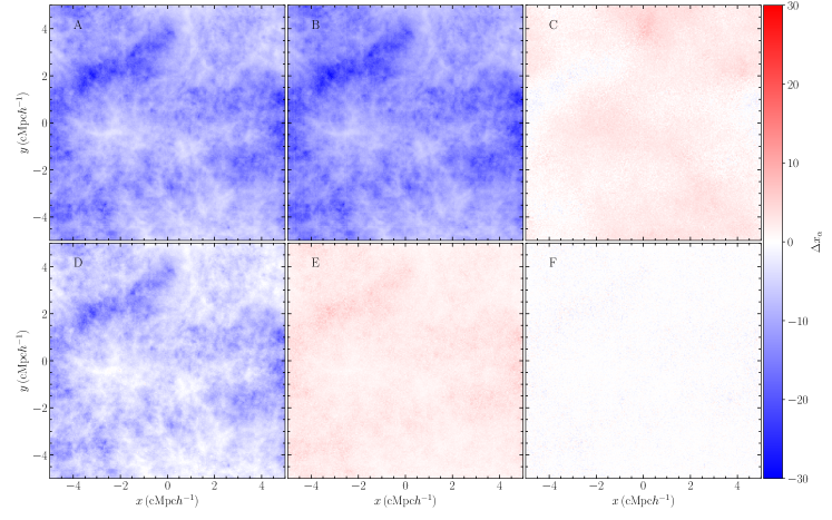
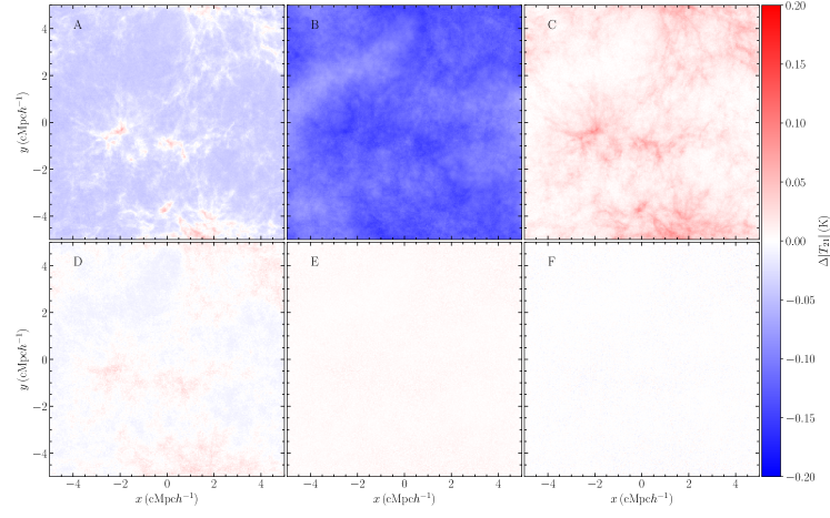
Figure 4: The relative importance of different ingredients of Ly $\alpha$ radiative transfer for the computation of Ly $\alpha$ coupling $x_{\alpha}$ (top) and 21-cm signal $T_{21}$ (bottom). The colour shows the difference $\Delta x_{\alpha}$ in the Ly $\alpha$ coupling (top) and $\Delta|T_{21}|$ in the 21-cm signal (bottom) between each of our specially designed simulations A to F and fiducial simulation. The quantities $\Delta x_{\alpha}$ and $\Delta|T_{21}|$ are averaged along the $\mathord{\mathchoice{\ooalign{$\displaystyle z$\cr\vrule height=2.05373pt,depth=-1.82124pt,width=2.29062pt\cr}\vphantom{\hbox{\set@color$\displaystyle z$}}}{\ooalign{$\textstyle z$\cr\vrule height=2.05373pt,depth=-1.82124pt,width=2.29062pt\cr}\vphantom{\hbox{\set@color$\textstyle z$}}}{\ooalign{$\scriptstyle z$\cr\vrule height=1.47249pt,depth=-1.24pt,width=1.60344pt\cr}\vphantom{\hbox{\set@color$\scriptstyle z$}}}{\ooalign{$\scriptscriptstyle z$\cr\vrule height=1.08498pt,depth=-0.8525pt,width=1.14531pt\cr}\vphantom{\hbox{\set@color$\scriptscriptstyle z$}}}}$ axis of the simulation box. The difference $\Delta x_{\alpha}$ is given by $x_{\alpha,i}-x_{\alpha,0}$, where $x_{\alpha,0}$ is the Ly $\alpha$ coupling from our fiducial simulation, and $x_{\alpha,i}$ is the Ly $\alpha$ coupling in each of the simulations A to F. (A similar definition is used for $\Delta|T_{21}|$). The simulations A to F are described in Table 1.

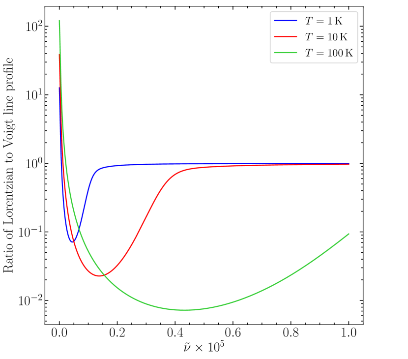
Figure 5: The ratio of Lorentzian and Voigt line profiles for Ly $\alpha$ photons at three different temperatures. The horizontal axis shows frequency in units of $\tilde{\nu}=(\nu-\nu_{\alpha})/\nu_{\alpha}$. For temperatures $\sim$100\text{\,}\mathrm{K}$$ the Lorentzian can be lower than Voigt by factors as high as 100. This explains the under prediction of Ly $\alpha$ coupling in configurations A and B.

Loeb & Rybicki (1999, LR99) considered RT of Ly $\alpha$ photons emitted by a point source in a uniform, homogeneous and neutral medium undergoing a Hubble expansion but at a zero temperature. In this framework, because of zero thermal velocity of atoms and absence of recoil, scattering does not change the photon frequency. Therefore, frequency changes only as a result of redshifting.

To our knowledge, CZ07 were the first to consider the effect of multiple scatterings of Ly $\alpha$ photons in the context of a 21-cm signal. However, similar to LR99 the RT algorithm was applied to a homogeneous medium having no thermal motions. Moreover, only wing scatterings (applicable to photons having large frequency offset) were considered.

The seminal work by S07 introduced a 3D RT code which could self-consistently be applied to real cosmological settings without recourse to assumptions like homogeneous density and zero temperature. They studied 3D RT for some idealised configurations such as a homogeneous medium with a point source at the centre, a high-density central clump at the centre or an isothermal density profile. Baek et al. (2009) applied the technology from S07 for the first time to real cosmological simulations. The period of cosmic history of interest in their work was the epoch of reionisation.

S07 and followup works by Baek et al. (2009) and Vonlanthen et al. (2011) assumed isotropic scattering whereas in our work we consider the more accurate phase function (Dijkstra & Loeb, 2008b). They assumed coherent scattering in the atom frame while we account for the recoil effect (equation 23). Finally, these authors have used acceleration schemes like core-skipping algorithms that we avoid in this work. When a photon is in its line core it undergoes a large number of scatterings over short distances. Often in MCRT codes, to speed up the computation, the photon is moved directly to the wings (Ahn et al., 2002). In particular, Baek et al. (2009) trigger core-skipping when the photon is within $10\Delta\nu_{\mathrm{D}}$ of the $\nu_{\alpha}$ and add $\sim 10^{6}$ scatterings ‘by hand’ at the same location. As has been recently pointed out by Semelin et al. (2023), core-skipping mechanisms inadvertently miss the effect of gas velocities in line core RT. The new code introduced in their work does not rely on such an algorithm and solves the RT throughout the line self-consistently. However, their code is applicable at 0 K and a medium of uniform scatterer density, similar to the LR99 set-up.

Another notable work that deals with Ly $\alpha$ RT is by Naoz & Barkana (2008). They calculate the specific intensity due to wing scatterings by inserting a ‘correction’ factor $f_{\mathrm{ws}}(n+1\to n,r_{z^{\prime}z})$. This factor would serve as a correction for photons of frequencies between Ly$n$ and Ly$(n+1)$ when the photon was emitted at a redshift $z^{\prime}$ and shifts into Ly $\alpha$ at $z$ such that the straight line distance is $r$ from the point of emission and the point where the photon becomes a Ly $\alpha$ photon.

Reis et al. (2021, 2022) further extended Naoz & Barkana (2008). They fit a general form of a function to the histogram which describes the number of photons in the logarithmic bin at $r$. However, as in LR99 or CZ07, Reis et al. (2021, 2022) do not account for the bulk motion of the gas, non-zero temperature effects (so that a Lorentzian line profile can be assumed and thermal motion can be ignored) or the cosmological hydrogen distribution but instead assumed it to be at the average value at the redshift of interest. Further, the scattering was assumed to be isotropic with no recoil.

In Fig. 3 we compared our results to a system which does not account for multiple scatterings at all. We now compare our results accounting for multiple scatterings of Ly $\alpha$ photons with results from specially designed simulations in which each time we invoke a specific RT assumption in effect, namely bulk motion, cosmological H i density, non-zero temperature, scattering direction and recoil. Table 1 shows the different configurations against which we make our comparisons. The simulations details remain the same as above. Throughout the following discussion, we refer to the results of the right-hand-side panels of Fig. 3 as our fiducial results.

The resulting Ly $\alpha$ coupling difference, $\Delta x_{\alpha}$, and difference in 21-cm signal magnitude, $\Delta|T_{21}|$, averaged along the $\mathord{\mathchoice{\ooalign{$\displaystyle z$\cr\vrule height=2.28192pt,depth=-2.02362pt,width=2.54515pt\cr}\vphantom{\hbox{\set@color$\displaystyle z$}}}{\ooalign{$\textstyle z$\cr\vrule height=2.28192pt,depth=-2.02362pt,width=2.54515pt\cr}\vphantom{\hbox{\set@color$\textstyle z$}}}{\ooalign{$\scriptstyle z$\cr\vrule height=1.6361pt,depth=-1.37779pt,width=1.7816pt\cr}\vphantom{\hbox{\set@color$\scriptstyle z$}}}{\ooalign{$\scriptscriptstyle z$\cr\vrule height=1.20554pt,depth=-0.94724pt,width=1.27257pt\cr}\vphantom{\hbox{\set@color$\scriptscriptstyle z$}}}}$ axis are shown in Fig. 4. We show $\Delta x_{\alpha}$ and $\Delta|T_{21}|$ in 6 different cases labelled A to F. We discuss each case in detail below, but Table 1 give the essential details. In Fig. 4, $\Delta x_{\alpha}$ is defined as $x_{\alpha,i}-x_{\alpha,0}$, where $x_{\alpha,0}$ is our Ly $\alpha$ coupling predicted in fiducial model (shown in the right column of Fig. 3) and $x_{\alpha,i}$ is that obtained for one of the A to F configurations. The quantity $\Delta|T_{21}|$ is defined similarly.

In configurations which require a non-cosmological density, we replace the $n_{\text{H\,{i}}}$ in all the cells of the simulation box to a constant value $186.6\text{\,}\mathrm{m}^{-3}$, which is the average neutral hydrogen density in our fiducial box. In cases involving non-zero gas temperature the temperature distribution is identical to the fiducial simulation. In particular configuration A is similar to what was used by Reis et al. (2021) where we do not account for bulk motion of scatterers, assume uniform $n_{\text{H\,{i}}}$, $T_{\mathrm{k}}=0$, use isotropic scattering and do not account for recoil. Configuration B is similar to what was used by Semelin et al. (2023) where we do account for the cosmological bulk motion but the other assumptions remain the same as for Reis et al. (2021).

Note that all of these assumptions refer only to the RT. So, for example assumptions such as uniform gas density or zero gas temperature employed in these numerical experiments will affect the RT computation of $x_{\alpha}(\bm{r},z)$, but when we compute the 21-cm signal, $T_{21}(\textbf{{r}},z)$, we still use the cosmological values $\delta(\bm{r},z)$ or $T_{\mathrm{k}}(\bm{r},z)$ obtained from our ramses simulation.

We now discuss each configuration in detail.

A

In this configuration we do not account for bulk motion, assume uniform $n_{\text{H\,{i}}}$, $T_{\mathrm{k}}=0$, do not account for recoil and assume isotropic scattering. From Fig. 4 we conclude that configuration A under-predicts the Ly $\alpha$ coupling compared to fiducial model. The reason is as follows. In a medium of non-zero temperature, photons close to the resonance will have a large scattering cross-section $\sigma$. Using a Lorentzian (the appropriate cross section at $T_{\mathrm{k}}=0$) for $\sigma$ will as a consequence significantly under-predict the number of scatterings and hence $x_{\alpha}$. Only for a small frequency range is the Lorentzian is greater than Voigt cross-section. As an example, at $T_{\mathrm{k}}=$100\text{\,}\mathrm{K}$$ and for a photon of frequency $\left(1+$5\text{\times}{10}^{-6}$\right)\nu_{\alpha}$ the Lorentzian is lower than Voigt function by a factor of $\sim 10^{2}$. (See Fig. 5.) This can under-predict the 21-cm signal as seen in Fig. 4; the box-averaged 21-cm signal is $-166.62\text{\,}\mathrm{mK}$. The RMS difference in the 21-cm signal magnitude compared to fiducial model is $77.7\text{\,}\mathrm{mK}$. Consequently, the relative difference (RMS) is 39.7 %.

B

Configuration B differs from A only in the inclusion of bulk motion. We find $x_{\alpha}$ is underestimated which also leads to an underestimation of $T_{21}$. This is explained more via configuration C. The box-averaged $T_{21}$ comes out to be the lowest, at a value of $-78.74\text{\,}\mathrm{mK}$. The RMS difference and the RMS relative difference in the 21-cm signal magnitude compared to fiducial model are $132.5\text{\,}\mathrm{mK}$ and 67.7 %, respectively.

C

We consider the effect of bulk motion more explicitly through configuration C. Configuration C differs from the fiducial model only in accounting of bulk motion. At $0\,$K (as in configuration B) the cross-section is a Lorentzian which is a sharply peaked function. Even though the comoving frequency smoothly decreases as a result of redshifting (by ensuring small enough $\delta l$) the cell frame frequency can have large jumps from point to point in space due to varying bulk velocities. This may cause the photon to miss essential scatterings if it is in the line core. This is the case for configuration B. However, this issue is diluted when bulk motion is taken into account in conjunction with non-zero temperature as the line profile is broader.

The box-averaged $T_{21}$ is $-213.06\text{\,}\mathrm{mK}$ compared to our $-195.60\text{\,}\mathrm{mK}$. The RMS difference and the RMS relative difference in the 21-cm signal magnitude compared to fiducial model are $71.6\text{\,}\mathrm{mK}$ and 36.6 %, respectively.

D

At first, the expression of rate of scatterings per atom, $P_{\alpha}$, suggests that it should be independent of number density (see equation 28). However, the number density variations affect the photon trajectories and hence $P_{\alpha}$, as evident in Fig. 4 panel D. In configuration D we use a uniform number density of hydrogen but everything else is same as in fiducial model. Though the box-averaged $T_{21}$ comes out to be $-195.86\text{\,}\mathrm{mK}$, which is close compared to our $\langle T_{21}\rangle=$-195.60\text{\,}\mathrm{mK}$$, the RMS difference is $68.8\text{\,}\mathrm{mK}$. This indicates a wide spread in the distribution of difference in the 21-cm signal. The RMS relative difference in the 21-cm signal magnitude compared to fiducial model is 35.2 %.

E

In this configuration everything is same as in the fiducial model except for recoil. Not including recoil overestimates $x_{\alpha}$ as evident in Fig. 4 panel E. This is mostly because with recoil included, the photons lose energy faster compared to the case when recoil is excluded. As a result ‘non-recoiling’ photons redshift out of the line core at a slower rate compared to recoiling photons. This allows non-recoiling photons to spend more time in the core thereby increasing the number of scatterings. Because we get a higher $x_{\alpha}$ we get a stronger 21-cm signal as evident in Fig. 4 panel E. The box-averaged $T_{21}$ comes out to be $-199.78\text{\,}\mathrm{mK}$ compared to our $-195.60\text{\,}\mathrm{mK}$. The RMS difference and the relative difference in the 21-cm signal magnitude compared to fiducial model are $44.8\text{\,}\mathrm{mK}$ and 22.9 %, respectively.

Note that accounting for recoil is an important physical mechanism to establish the thermal equilibrium between the Ly $\alpha$ photons and the gas. It is this process which sets the colour temperature, $T_{\alpha}$, to the gas temperature (Seon & Kim, 2020). When we calculate the spin temperature in configuration E we assume $T_{\alpha}=T_{\mathrm{k}}$.

F

In this configuration everything is same as in fiducial model except for the scattering phase function. Here we use a uniform function as appropriate for isotropic scattering. The box-averaged $T_{21}$ in this configuration is $-195.86\text{\,}\mathrm{mK}$ compared to our $-195.60\text{\,}\mathrm{mK}$. The RMS difference and the RMS relative difference in the 21-cm signal magnitude compared to fiducial model are $61.6\text{\,}\mathrm{mK}$ and 31.5 %, respectively.

In general all 5 ingredients are important for Ly $\alpha$ RT and consequently the tomographic 21-cm signal as suggested by the large RMS difference in each case. However, at the first level of approximation a cosmological $n_{\text{H\,{i}}}$, recoil and anisotropy are sub-dominant when a box-averaged 21-cm signal is desired as the mean difference is small between fiducial model and D, E or F. The mean percentage difference in the 21-cm signal is not more than $2\,$% in any of these configurations.

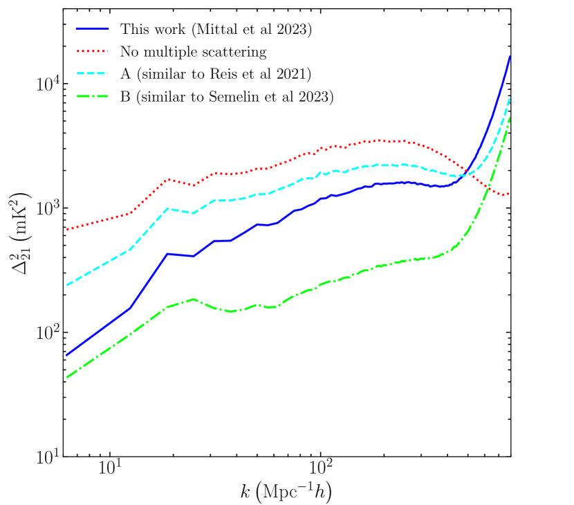
Figure 6: The 21-cm power spectrum $\Delta^{2}_{21}$ for cosmic dawn like conditions in our fiducial simulation. We show here results for four different cases as follows. The blue-solid and red-dotted curves correspond to results accounting for multiple scatterings and no multiple scatterings, respectively; Fig. 3 shows the 21-cm maps for these. Cyan-dashed and green-dash-dotted curves correspond to multiple scatterings of configurations A and B, respectively.

3.2 21-cm power spectrum

We next investigate how the fluctuations in 21-cm signal differ in different configurations. In our work there are three major contributors to the total 21-cm fluctuations, viz., gas temperature, density and Ly $\alpha$ scattering as evident from the 21-cm expression in equation (1). (As hydrogen is mostly neutral and uniform throughout, $x_{\text{H\,{i}}}$ fluctuations have a negligible contribution.) See Fig. 6 where we show results in terms of $\Delta^{2}_{21}\,(\mathrm{mK}^{2})$ as a function of physical wavenumber $k\,(\mathrm{Mpc}^{-1}h)$.

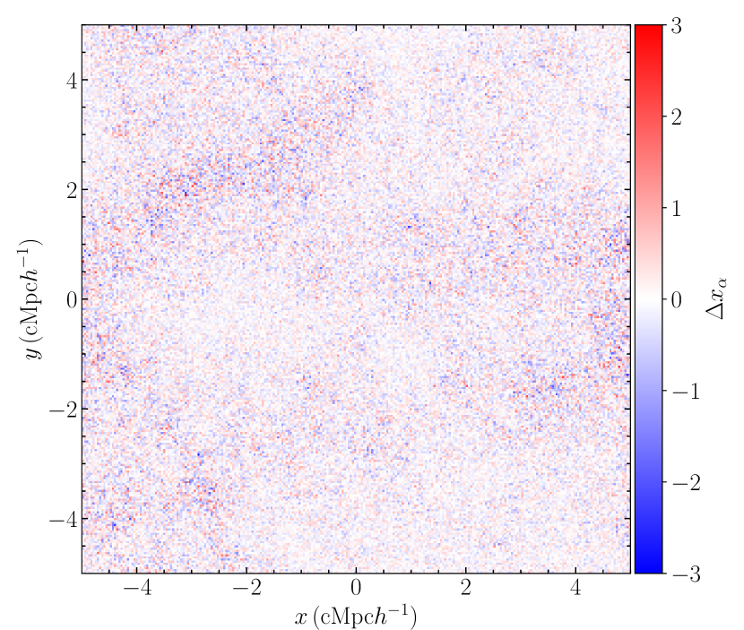
Figure 7: Projected average of $\Delta x_{\alpha}$ along the full depth in $\mathord{\mathchoice{\ooalign{$\displaystyle z$\cr\vrule height=2.05373pt,depth=-1.82124pt,width=2.29062pt\cr}\vphantom{\hbox{\set@color$\displaystyle z$}}}{\ooalign{$\textstyle z$\cr\vrule height=2.05373pt,depth=-1.82124pt,width=2.29062pt\cr}\vphantom{\hbox{\set@color$\textstyle z$}}}{\ooalign{$\scriptstyle z$\cr\vrule height=1.47249pt,depth=-1.24pt,width=1.60344pt\cr}\vphantom{\hbox{\set@color$\scriptstyle z$}}}{\ooalign{$\scriptscriptstyle z$\cr\vrule height=1.08498pt,depth=-0.8525pt,width=1.14531pt\cr}\vphantom{\hbox{\set@color$\scriptscriptstyle z$}}}}$ axis. We compare our fiducial run with $N_{\mathrm{mc}}=10^{8}$ against that done with $N_{\mathrm{mc}}=2\times 10^{8}$. The mean difference is $\sim\mathrm{10^{-4}}$ and RMS $\approx 6.6$. The box-averaged 21-cm signal for higher MC photons comes out to be $-202.91\text{\,}\mathrm{mK}$ compared to $-195.60\text{\,}\mathrm{mK}$ for a lower MC photon count. See text for more details.

At $k=6\,\mathrm{Mpc}^{-1}h$ we have $\Delta^{2}_{21}\approx$66\text{\,}\mathrm{m}\mathrm{K}^{2}$$ for our fiducial model. $\Delta^{2}_{21}(k)$ increases monotonically towards large $k$. The blue-solid curve corresponds to our fiducial simulations. A similar monotonic trend is seen for power spectra corresponding to configurations A and B shown in cyan-dashed and green-dash-dotted curves, respectively. The red-dotted curve corresponds to the no-multiple-scatterings case, which moves downwards at small scales (large $k$). This is mostly because of the smoother coupling and signal distribution in the domain thereby misses the small-scale inhomogeneities. An overall downward shift exists for the green-dashed curve because of its lower box-averaged $T_{21}$.

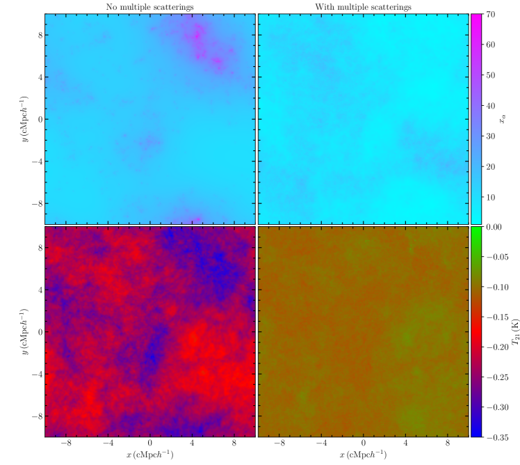
Figure 8: Effect of the box size on our results. This figure has the same quantities as for Fig. 3, but for a box of size $20\,\mathrm{cMpc}h^{-1}$ with $512^{3}$ cells. Note that the colour bar ranges are different than those in Fig. 3. The box-averaged 21-cm signal for left- and right-hand sides are $\langle T_{21}\rangle=$-236.97\text{\,}\mathrm{mK}$$ and $-101.53\text{\,}\mathrm{mK}$, respectively.

4 Possible future improvements

The above results indicate the effect that RT has on Ly $\alpha$ coupling at cosmic dawn. The results also help us understand the relative importance of various gas properties in setting the Ly $\alpha$ coupling. Nonetheless, we can now identify possible future improvements. These include improvements in the simulation box size, number of MC photons, spatial and mass resolution, and the MCRT stopping criterion. We now discuss each of these points.

Perhaps the most important factor which decides convergence of RT simulations is the number of MC photons $N_{\mathrm{mc}}$. As is generally true for MC process, an MCRT simulation result would suffer from sampling noise. Following Semelin et al. (2023), the relative error in our Ly $\alpha$ coupling, when a broad Voigt-like line profile and periodic boundary conditions are used, can be estimated to be $\eta=\sqrt{N_{\mathrm{cell}}/(N_{\mathrm{eff}}N_{\mathrm{mc}})}$, where $N_{\mathrm{cell}}$ is the number of cells in the simulation box and $N_{\mathrm{eff}}$ is the average effective number of times an MC photon is seen in the box until the medium becomes transparent. We did our main runs with $N_{\mathrm{cell}}=256^{3}$ and $N_{\mathrm{mc}}=10^{8}$; we found that photons on an average loop over the box 21 times, so that $N_{\mathrm{eff}}=22$ which gives $\eta\approx 8.7\,$%. In order to get reasonably convergent results with, say, $\eta=1\,$% accuracy one would require $N_{\mathrm{mc}}\approx 8\times 10^{9}$. A simulation with these many number of photons can be prohibitively costly and thus, has been left for future. Nevertheless, we run a simulation with $2\times 10^{8}$ MC photons and compare the results with our fiducial model for which we used $10^{8}$ MC photons.

Figure 7 shows the difference, $\Delta x_{\alpha}$, in Ly $\alpha$ coupling using $10^{8}$ and $2\times 10^{8}$ MC photons. We define $\Delta x_{\alpha}$ as $x_{\alpha,1}-x_{\alpha,0}$, where $x_{\alpha,0}$ and $x_{\alpha,1}$ are the Ly $\alpha$ couplings with $10^{8}$ (the fiducial run, shown in the right-hand side column of Fig. 3) and $2\times 10^{8}$ MC photons, respectively. The mean and RMS of the difference over the complete domain are $\langle\Delta x_{\alpha}\rangle=5.8\times 10^{-4}$ and $\sqrt{\langle(\Delta x_{\alpha})^{2}\rangle}=6.6$, respectively. As to the spatial distribution of $\Delta x_{\alpha}$, we find that closer to the source the difference is somewhat smaller while it increase farther away from it. This is understandable as closer to the emission point the MC photon density is higher thereby reducing the MC noise. The box-averaged 21-cm signal comes out to be $\langle T_{21}\rangle=$-202.91\text{\,}\mathrm{mK}$$ compared $-195.60\text{\,}\mathrm{mK}$ when $10^{8}$ MC photons are used.

We next investigate the effect of simulation box size. Consider a box of side length $20\,\mathrm{cMpc}h^{-1}$ with $512^{3}$ cells. This set-up differs from our fiducial model in terms of box length and number of cells but has the same resolution of $39\,\mathrm{ckpc}h^{-1}$. Since the simulation box is different, we rerun our halo finder to find the sources and luminosity. We find a total of 1544 haloes (cf. our fiducial configuration where we had 213 haloes) and luminosity, $L=$7.1\text{\times}{10}^{56}\text{\,}\mathrm{s}^{-1}$$ (which is 8 times our fiducial model value; equation 14). We show results in Fig. 8. The box-averaged 21-cm signal without and with multiple scatterings is $-236.97\text{\,}\mathrm{mK}$ and $-101.53\text{\,}\mathrm{mK}$, respectively. We used different initial conditions so that we have a different density and temperature distribution compared to that shown in Fig. 1. As we have increased the number of cells but kept the MC photon count the same, this result suffers from a larger MC sampling noise.

Third, the spatial and mass resolution of the simulation can also be improved. Our fiducial simulation has a spatial resolution of $39\,\mathrm{ckpc}h^{-1}$ and the minimum halo mass resolved by the simulation is $1.96\times 10^{8}\,\mathrm{M}_{\odot}h^{-1}$. It remains to be understood how unresolved gas density structures affect the Ly $\alpha$ RT. The halo mass resolution also should ideally extend down to the uncertain star formation threshold at cosmic dawn. While the technology presented in this paper is now potentially capable of answering these questions, the computational expense involved forces us to leave resolution improvements to future work.

Finally, we used the stopping criterion of $x_{\mathrm{cell,crit}}=-6$. As mentioned in section 2.3.2, for this choice of critical frequency, the critical cross-section is $\sim 10^{-4}$ times central cross-section. By running test cases with successively higher $-x_{\mathrm{cell,crit}}$ (at fixed $N_{\mathrm{mc}}$, box size, and resolution) we found that going beyond $x_{\mathrm{cell,crit}}\approx-6$ to conditions such as $x_{\mathrm{cell,crit}}=-16$ has less than a per cent impact on the 21-cm signal. However, it remains to be explored the convergence of MCRT simulation in terms of $-x_{\mathrm{cell,crit}}$ combined with other possible improvements mentioned above.

By bringing greater realism in the treatment of gas physics, this work provides a starting point for a more accurate computation of Ly $\alpha$ coupling and the 21-cm signal, keeping the above considerations in mind.

5 Conclusions

In this work we have set up the technology to study multiple scatterings effect of Ly $\alpha$ photons for the computation of tomographic cosmological 21-cm signal at cosmic dawn. Using the AMR code ramses we performed hydrodynamical simulations to obtain the cosmological boxes giving us the density, temperature and bulk velocity of the gas. We post-processed our simulation with the rascas code to compute the propagation of Ly $\alpha$ photons with multiple scatterings using a Monte Carlo radiative transfer simulation. We modified rascas to account for the cosmological redshifting of photons and to compute the scattering rate using a path-based method. In contrast with previous works, we also account for recoil and anisotropic scattering, and more importantly, do not use core-skipping algorithms.

We investigate the role of multiple scatterings of Ly $\alpha$ photons due a finite spread of line profile against the traditional computation which implicitly assumes a Dirac-delta line profile. We also study the role played by different gas properties such as non-zero temperature, cosmological number density and bulk velocity in establishing the Ly $\alpha$ coupling and the 21-cm signal at cosmic dawn. Our main findings in this work are as follows.

1. Ly $\alpha$ coupling and consequently the 21-cm signal differ significantly when multiple scatterings are taken into account compared to the traditional calculations where no multiple scatterings are considered. The 21-cm signal in our fiducial simulation differs from the results of a traditional calculation by about 40 % (RMS).

2. Our treatment brings greater realism in how intergalactic gas physics is modelled in the computation of the Ly $\alpha$ RT. For example, previous work in the literature that modelled multiple scatterings of Ly $\alpha$ photons ignored effects of non-zero gas temperature. As a result these attempts reported a smaller value of the Ly $\alpha$ coupling $x_{\alpha}$ relative to our fiducial model. This is largely because a Lorentzian cross-section has a lower value compared to Voigt in the line core for a large part of frequency space where most scatterings happen. This under-predicts $x_{\alpha}$ and hence the 21-cm signal. In particular, our results in terms of 21-cm signal differ by 40 and 68 % (RMS), respectively from the radiative transfer computations comparable to those of Reis et al. (2021) and Semelin et al. (2023).

3. We investigate the relative importance of the gas bulk motion, cosmological H i density distribution, non-zero gas temperature, anisotropic scattering, and recoil, for Ly $\alpha$ RT. We conclude that the gas bulk motion and the non-zero gas temperature are the most important of these gas properties.

4. In agreement with previous authors, we find that Ly $\alpha$ RT reduces the 21-cm power spectrum at large scales, although the decrement in our simulations is less compared to previous RT models.

The global 21-cm signal is a promising probe for the thermal state of the universe at cosmic dawn. Accurate inferences from its measurements are valuable for a range of astrophysical and cosmological processes such galaxy formation, initial mass function of the first stars, nature of dark matter among others. This work offers an understanding of the various radiative transfer effects in increasing the accuracy in the modelling of Lyman-$\alpha$ coupling and hence the 21-cm signal. This work paves the way forward for better modelling and inferring from future experiments such as REACH.

Data Availability

The modified version of rascas developed by us for this work, along with the parameter files to reproduce the main results of this work will be made public soon. Additional codes to analyse the outputs, and parameter files to run music and ramses are available at https://github.com/shikharmittal04/lyman-a.

Appendix A Code Tests

In this appendix we present some tests of our version of the rascas code. The first two tests are the standard spectra reproducible by a non-Hubble-expanding version of the code, while the remaining four are the newer tests we did for testing our modified code for the scattering rate and/or Hubble expansion.

Unless stated otherwise in all of the following tests we do not account for the bulk motion of the scatterers or recoil, and assume an isotropic scattering. Because of the latter condition the phase function is simply given by $\mathcal{P}(\mu)=1$ as opposed to equation (20) which we have used in the main results of this paper. Finally note that we do not assume periodic boundary conditions for these tests and stop the photon propagation when it just crosses the domain boundary. We run all our tests on a $256^{3}$ grid box.

A.1 Effect of recoil on the output spectrum from a static medium

In this test we investigate how the recoil affects the output spectrum from a uniform, non-absorbing, static, optically thick sphere with a point source sitting at the centre emitting at the Lyman-$\alpha$ frequency. The analytical solution in the absence of recoil is given by (Dijkstra et al., 2006)

$$J(x)=\sqrt{\frac{\pi}{6}}\frac{1}{4a\tau_{0}}\frac{x^{2}}{1+\cosh\left(\sqrt{\frac{2\pi^{3}}{27}}\frac{|x|^{3}}{a\tau_{0}}\right)}\,,$$ (36)

valid for a large line centre optical depth from the centre of sphere to its boundary, $\tau_{0}=N_{\text{H\,{i}}}\sigma(\nu_{\alpha})$. Here $x$ is the frequency deviation form the line centre in Doppler units and $a$ is the Voigt parameter defined as the ratio of natural to Doppler line width. For Ly $\alpha$ scattering off hydrogen atoms

$$a=4.71\times 10^{-4}\left(\frac{T}{${10}^{4}\text{\,}\mathrm{K}$}\right)^{-1/2}\,,$$ (37)

and

$$\tau_{0}=8.3\times 10^{6}\left(\frac{N_{\text{H\,{i}}}}{$2\text{\times}{10}^{24}\text{\,}\mathrm{m}^{-2}$}\right)\left(\frac{T}{$2\text{\times}{10}^{4}\text{\,}\mathrm{K}$}\right)^{-1/2}\,,$$ (38)

for a uniform temperature $T$. The column density, $N_{\text{H\,{i}}}$, is set by the number density of hydrogen and the system size, in this case the sphere radius $(r)$, so that $N_{\text{H\,{i}}}=n_{\text{H\,{i}}}r$.

The spectrum given by equation (36) is normalised such that

$$\int_{-\infty}^{\infty}J(x)\,\mathrm{d}x=\frac{1}{4\pi}\,.$$ (39)

Figure 9 shows our results. We first note that the simulation result without recoil is in an excellent agreement with the analytical solution, as also established in Michel-Dansac et al. (2020). More importantly the figure illustrates the effect of recoil on the photons. In a static Universe and in the absence of recoil a photon is equally likely to get a positive and a negative Doppler shift on every scattering because of random thermal motion of scatterers. However, with recoil taken into account the frequency shifts are no longer unbiased; photons lose a small amount of energy to the scatterers. Hence, there are more photons with low energy which explains the enhanced left-hand-side peak.

For interested readers the following are our set-up parameters. The medium is at $T=$100\text{\,}\mathrm{K}$$, number density of neutral hydrogen is $n_{\text{H\,{i}}}=$3.477\text{\times}{10}^{17}\text{\,}\mathrm{m}^{-3}$$ and radius of the sphere is $r=$4.9\text{\times}{10}^{5}\text{\,}\mathrm{m}$$ so that $N_{\text{H\,{i}}}=$1.7\text{\times}{10}^{23}\text{\,}\mathrm{m}^{-2}$$ and the line centre optical depth is $\tau_{0}=10^{7}$. We run our simulation for $10^{6}$ Monte Carlo (MC) photons. We normalise the resulting numerical histogram, using 100 bins, according to equation (39).

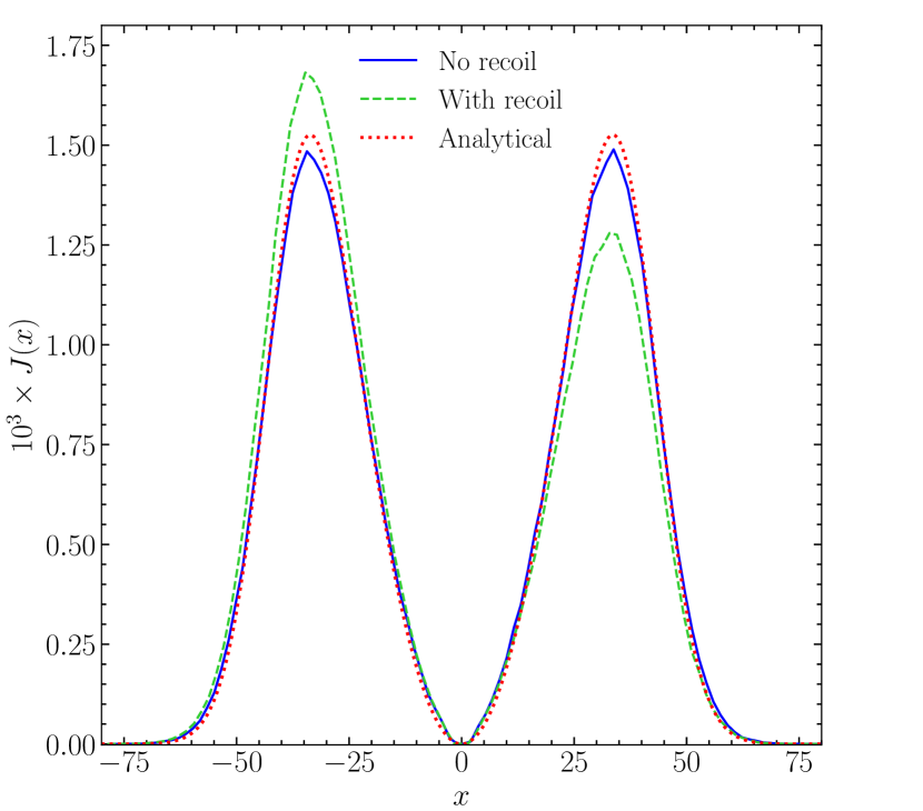
Figure 9: The figure shows the output spectrum normalised to $1/4\pi$ from a homogeneous static sphere with a point source emitting from the centre at Ly $\alpha$ frequency. The medium temperature and the line centre optical depth are $100\text{\,}\mathrm{K}$ and $\tau_{0}=10^{7}$, respectively. The red dotted curve shows the analytical solution (Dijkstra et al., 2006) applicable to a medium with large optical depths such as in this case. Blue-solid curve shows the output predicted by running a rascas simulation when no recoil is taken into account. The agreement between the two curves shows an agreement between the analytical solution and numerical simulation. With recoil the spectrum is asymmetric as shown by the green-dashed curve.

A.2 Radially- vs Hubble-expanding medium

Here we highlight the difference between output spectra from a medium simply given a radial dilation vs that from a Hubble-expanding medium. Our radially-expanding medium is similar to the previous configuration except this time the medium has an additional bulk motion. The velocity increases linearly with radius from 0 at the centre of sphere to $v_{\mathrm{max}}=\mathcal{H}r$ at the outermost shell, just as in the set-up of Laursen et al. (2009). In such a system the photons that are initially Doppler shifted to higher frequency due to random thermal motion of scatterers, on reaching larger radii (when radially outwards velocity becomes large) will appear closer to the line centre to scatterers. These photons have a high scattering rate compared to the initially redder photons which become even redder when reaching larger radii. Thus, more redder photons escape the boundary than the bluer ones which results in an asymmetric spectrum. We firstly note that the output from this system matches with that of Laursen et al. (2009) as shown in Fig. 10.

Let us now consider Hubble-expanding medium. While equation (26) at first seems to suggest redshifting can be captured by Doppler shifting the photon by giving the scatterer precisely the Hubble velocity, it is only applicable when the mean free path is small. An alternative and perhaps the best way to understand why the two cases are different is through the following thought experiment. Let us label the two cases as ‘radial’ version and ‘Hubble’ version for ease of discussion. Consider a very rare scenario where a photon moves from the centre to boundary without scattering even once. In radial version photon will exit the sphere with the same frequency as its emission frequency because it never touched an atom which could have caused a frequency shift. But in Hubble version the photon undergoes a cosmological redshift which has nothing to do with the presence of atoms and hence the photon exits with a lower frequency than it originally started with (Dijkstra et al., 2006).

From the above discussion it is clear that radially-expanding and a Hubble-expanding medium will produce different outputs. As evident from Fig. 10 the output spectrum from a Hubble-expanding medium (green dashed curve, labelled ‘Hubble expansion’) is slightly more shifted compared to that from a radially expanding medium (blue solid curve, labelled ‘Radial expansion’) in accordance with our expectation. Additionally, we conclude that to capture the cosmological redshifting, it is better to work in a comoving frame where one redefines photon frequency in gas frame (according to equation 26) over predetermined small distances traversed by the photon while in free propagation.

For interested readers the following are our set-up parameters. The medium has a uniform neutral hydrogen density of $n_{\text{H\,{i}}}=$3.84\text{\times}{10}^{3}\text{\,}\mathrm{m}^{-3}$$, a constant temperature of $T=${10}^{4}\text{\,}\mathrm{K}$$ and a radius $1.69\text{\times}{10}^{-2}\text{\,}\mathrm{Mpc}$. The column density and line centre optical depth are $N_{\text{H\,{i}}}=$2\text{\times}{10}^{24}\text{\,}\mathrm{m}^{-2}$$ and $\tau_{0}\approx 1.2\times 10^{7}$, respectively. For $\mathcal{H}=$1184.23\text{\,}\mathrm{k}\mathrm{m}\mathrm{s}^{-1}\mathrm{M}\mathrm{pc}^{-1}$$ the maximum velocity – which is at the edge of the sphere – is $20\text{\,}\mathrm{k}\mathrm{m}\mathrm{s}^{-1}$. We run our simulation for $10^{6}$ MC photons. We normalise the resulting numerical histogram, using 100 bins, according to equation (39).

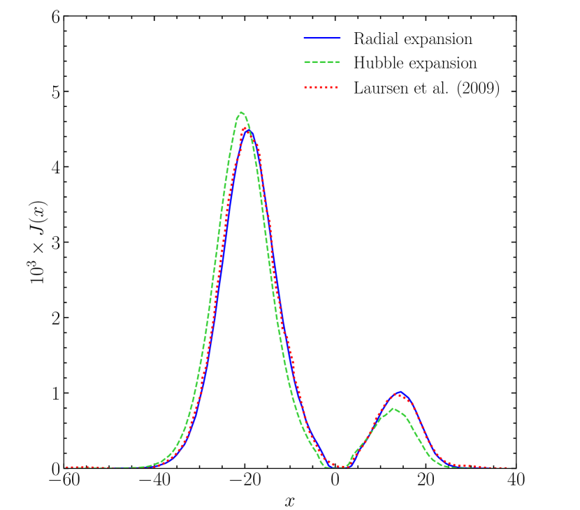
Figure 10: We reproduce the result of fig. 8 of Laursen et al. (2009) and also illustrate how a true Hubble-expanding medium differs from a medium in which the atoms are given an additional Hubble-flow-like velocity field. Our set-up has a point source at the centre of our sphere emitting at Ly $\alpha$ frequency. The medium temperature, column density and the edge velocity are ${10}^{4}\text{\,}\mathrm{K}$, $N_{\text{H\,{i}}}=$2\text{\times}{10}^{24}\text{\,}\mathrm{m}^{-2}$$ and $v_{\mathrm{max}}=$20\text{\,}\mathrm{k}\mathrm{m}\mathrm{s}^{-1}$$, respectively. The red-dotted curve shows the result from previous literature, the blue solid curve shows the result from a medium given a radial dilation and the green dashed curve represents output from a truly Hubble-expanding medium. Hubble expansion results in a higher frequency shift because of which the green curve is more leftwards than blue one.

A.3 Scattering rate in a non-Hubble-expanding medium

Here we run our first test for the scattering rate per atom by comparing with the results from Seon & Kim (2020). rascas version introduced in Michel-Dansac et al. (2020) did not have the $P_{\alpha}$ calculation capabilities. We have introduced this in our version.

The set-up is similar to the previous cases where we have a monochromatic source emitting at Ly $\alpha$ frequency from the centre of sphere. The column density is $1.69\text{\times}{10}^{19}\text{\,}\mathrm{m}^{-2}$ and the temperature is $100\text{\,}\mathrm{K}$ giving us a line centre optical depth of $\tau_{0}=10^{3}$. We run our simulations for two sub-cases – i) where we have a static medium, and ii) where medium is expanding outwards (not Hubble) with the outermost velocity being $10\text{\,}\mathrm{k}\mathrm{m}\mathrm{s}^{-1}$. We make a radial profile of $P_{\alpha}$ to facilitate a comparison with previous work. For our numerical set-up we used $10^{7}$ MC photons and 80 histogram bins for the radial profile.

As evident from Fig. 11 we match reasonably well with results from previous literature. As the source strength is irrelevant for this test case we show a normalised version of $P_{\alpha}$ such that $P_{\alpha}=1$ at the farthest distance from the source. Also, we normalise the distance with the sphere radius. Solid and dashed curves are ours and their results, respectively.

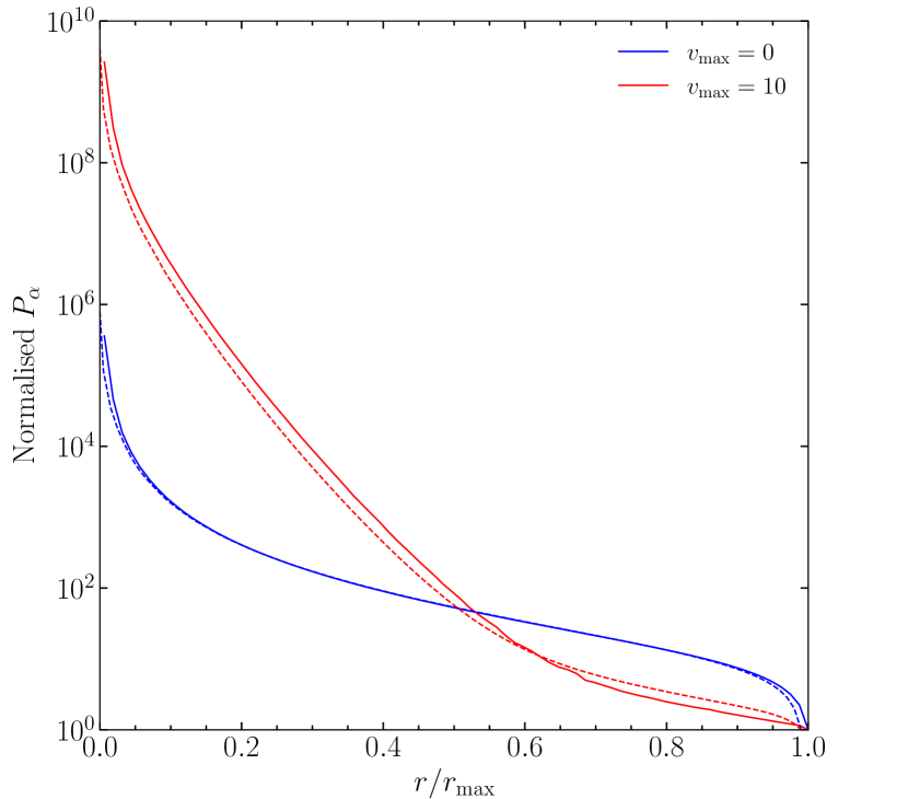
Figure 11: Spherically-averaged radial profile of scattering rate $P_{\alpha}$ in a medium of uniform density and temperature ($100\text{\,}\mathrm{K}$) with a single source emitting at Ly $\alpha$ frequency from the centre. The line centre optical depth is $\tau_{0}=10^{3}$. The blue and red curves correspond to a static and radially expanding media, respectively. $v_{\mathrm{max}}$ indicates the maximum velocity observed at the spherical boundary in units of $\mathrm{k}\mathrm{m}\mathrm{s}^{-1}$. The solid curves, results from our own simulations, match reasonably well with the dashed curves which are the results by Seon & Kim (2020).

A.4 Spectrum in a Hubble-expanding medium

Here we reproduce the analytical solution given by Loeb & Rybicki (1999, LR99). In this set-up the spherical medium undergoes a Hubble expansion and is at absolute zero. The consequence of the latter is that the gas atoms do not have any thermal motion and the line profile of the Ly $\alpha$ photons is simply given by a Lorentzian as follows

$$\sigma_{\mathrm{L}}(\nu)=\frac{3\lambda_{\alpha}^{2}}{2\pi}\frac{\tilde{A}^{2}}{(\nu-\nu_{\alpha})^{2}+\tilde{A}^{2}}\,,$$ (40)

where $\tilde{A}=A_{21}/(4\pi)$. However, to be exactly consistent with LR99 radiative transfer physics we use the wing approximation to the above form, i.e.

$$\sigma_{\mathrm{L}}(\nu)\approx\frac{3\lambda_{\alpha}^{2}}{2\pi}\frac{\tilde{A}^{2}}{(\nu-\nu_{\alpha})^{2}}\,.$$ (41)

We place our source at the centre of the sphere emitting at the frequency of Ly $\alpha$, i.e. $\nu=\nu_{\alpha}$. Because of the absence of thermal motion and recoil, frequency is not affected by scattering but changes merely due to redshifting. Note that contrary to the previous set-up, this time we have a true Hubble expansion.

The analytical solution for the set-up described above is given by

$$\tilde{J}(\tilde{\nu},\tilde{r})=\frac{1}{4\pi}\left(\frac{9}{4\pi\tilde{\nu}^{3}}\right)^{3/2}\exp\left(-\frac{9\tilde{r}^{2}}{4\tilde{\nu}^{3}}\right)\,,$$ (42)

where $\tilde{r}=r/r_{\star}$ and $\tilde{\nu}=(\nu_{\alpha}-\nu)/\nu_{\star}$, where $\nu_{\star}$ is a convenient frequency scale introduced by LR99 for which a photon initially at frequency $\nu_{\alpha}-\nu_{\star}$ has an optical depth 1 out to infinity. Similarly, $r_{\star}$ is the proper distance from the source where the Hubble expansion produces a frequency shift of $\nu_{\star}$.

For our numerical set-up we prepare a 2D histogram of 1000 bins in both, $\tilde{r}$ and $\tilde{\nu}$ space. We increment the bin value by 1 corresponding to photon’s current position and frequency as the photon is made to propagate over small distances. We run our simulations at $z=10$ for which $\nu_{\star}=$1.2\text{\times}{10}^{13}\text{\,}\mathrm{Hz}$$, $r_{\star}=$3.22\text{\times}{10}^{22}\text{\,}\mathrm{m}$$ and assigned uniform density of $254\text{\,}\mathrm{m}^{-3}$. We normalise our numerical histogram such that the peak of our numerical result coincides with that of analytical curve. We use $10^{7}$ MC photons for this test.

Figure 12 shows results from our general purpose MCRT code compared with the analytical solution, equation (42). We find reasonable agreement between the two.

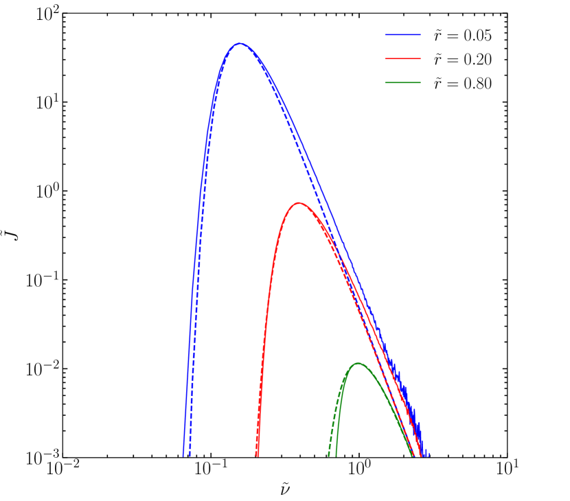
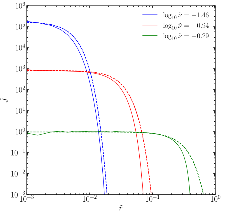
Figure 12: We demonstrate that our radiative transfer simulation reproduces the analytical solution by Loeb & Rybicki (1999) (equation 42) for the specific intensity, $\tilde{J}=\tilde{J}(\tilde{r},\tilde{\nu})$, in a spherical medium of uniform number density of scatterers undergoing Hubble expansion at a temperature of $0\text{\,}\mathrm{K}$ (so that the line profile is given by a Lorentzian and the scatterers have no thermal motion). A single source emits at Ly $\alpha$ frequency from the centre of the sphere. Left panel: $\tilde{J}$ as a function of non-dimensionalised frequency, $\tilde{\nu}$, at fixed radii. Right panel: $\tilde{J}$ as a function of non-dimensionalised radius, $\tilde{r}$, at fixed frequencies. In both panels the solid curves show our results and the dashed curves show the analytical solution. See text for more details.

A.5 Scattering rate in a Hubble expanding medium

For our final test we reproduce the $r^{-2.3}$ and $r^{-2}$ behaviour of the radial profile of $P_{\alpha}$ at small radii and large radii, respectively by a source which has a flat SED in a spherical medium of uniform hydrogen number density. See CZ07 for an explanation for this trend. We emphasise that $r^{-2.3}$ behaviour is seen only with the current SED type. Variations in the SED results in slight deviations from $r^{-2.3}$ behaviour.

The following are our set-up details. We set the radius of the sphere to $100\,\mathrm{cMpc}$ and hydrogen number density at $254\text{\,}\mathrm{m}^{-3}$, which is the average value at $z=10$ for our cosmological parameters. We place the source at the centre with flat SED – in terms of number of photons per unit frequency bin. Just as in the previous test we work at $0\text{\,}\mathrm{K}$ so that the line profile is a Lorentzian and gas atoms have no thermal motion. We used $10^{7}$ MC photons and 50 histogram bins for the radial profile.

We recover the $r^{-2.3}$ and $r^{-2}$ behaviour of $P_{\alpha}=P_{\alpha}(r)$ at small and large radii, respectively, in agreement with S07 and/or CZ07 as evident in Fig. 13. The blue-solid line shows the result from our simulation. (The minor deviation from $r^{-2}$ visible can be fixed by considering even larger radii). Just as for our third test run we show only a normalised version of $P_{\alpha}$ such that $P_{\alpha}=1$ at the farthest distance from the source.

As a further sanity check of our MCRT implementation we find that on setting a Dirac-delta line profile we recover $r^{-2}$ trend of $P_{\alpha}(r)$ (green circles). As to why this should be the case can be seen as follows. A Dirac-delta line profile implies that multiple scatterings of Ly $\alpha$ are ignored. In this case the photon only scatters when it is exactly at the line centre frequency. Given an initial frequency one can compute the distance covered $r$ before they redshift and reach the line centre from the source. All photons of the same initial frequency will cross the sphere of radius $r$ at the same time and thus, the ‘Ly $\alpha$’ flux and hence the scattering rate is simply proportional to $L/4\pi r^{2}$, where $L$ is the source luminosity (see also Dijkstra & Loeb, 2008a). This implicit assumption for the calculation of background specific intensity has been used in 21-cm literature previously.

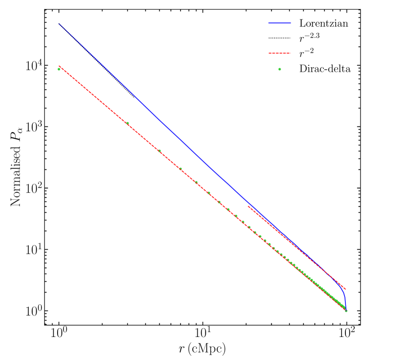
Figure 13: Spherically-averaged profile of scattering rate $P_{\alpha}$. At small and large radius we recover the $r^{-2.3}$ and $r^{-2}$ behaviour, respectively when a Lorentzian line profile is used (blue-solid curve), consistent with previous literature. The medium is maintained at a uniform density and $0\text{\,}\mathrm{K}$ with a single source emitting from the centre with a flat SED in terms of number by frequency extending from Ly $\alpha$ to Ly $\beta$. We also recover the $r^{-2}$ behaviour (green circles) when the line profile is replaced by a Dirac-delta function. Red-dashed and black-dotted lines are guides representing slopes of $-2$ and $-2.3$ (on log-log scale), respectively. The different curves are separated only for clarity; the vertical positioning is unimportant.

Appendix B Path-based vs point-based scattering rate

In this section we investigate two different styles of computing the scattering rate per atom, $P_{\alpha}$. In the first method we compute $P_{\alpha}$ by counting the number of scatterings in each cell while in the second method we sum the total optical depth traversed by all the photons in each cell. Throughout this work we have used the second definition even though the first one better aligns with the meaning of $P_{\alpha}$. The second version is an approximation to the first one and in general is accurate in regions of low optical depths (Seon & Kim, 2020).

We follow the second definition because it gives a smoother version of $P_{\alpha}$, and hence $x_{\alpha}$. A photon will pass through several cells but scatter in a much smaller number of cells. First version will give non-zero $P_{\alpha}$ only in cells where scattering occurred while second version gives a non-zero $P_{\alpha}$ in all the cells through which the photon passed. Thus, the second version gives an ‘interpolated’ map of the first version. As an example, for the toy model shown in Fig. 2 the first version of $P_{\alpha}$ would give $P_{\alpha}(c_{1})=0$ and

$$P_{\alpha}(c_{2})=\frac{L/2}{V_{c_{2}}n_{\text{H\,{i}},c_{2}}}\times 2\,.$$

This clearly shows that first version may lead to abrupt variations in $P_{\alpha}$ and the derived quantities.

When the number of MC photons is large the difference between the two versions is expected to be small as evident through Fig. 14. Also, note that the error is somewhat higher in regions of high density as they have large optical depth compared to low density areas. This is consistent with the approximation which leads to the $2^{\text{nd}}$ version from the $1^{\text{st}}$ one (see Seon & Kim, 2020). Since the overall error is small and leads to even smaller effect on the 21-cm signal we work with the second version of $P_{\alpha}$.

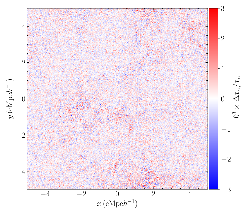
Figure 14: Projected average of the relative difference between Ly $\alpha$ coupling, $(x_{\alpha,2}-x_{\alpha,1})/x_{\alpha,1}$, because of two different versions of $P_{\alpha}$, where $x_{\alpha,1,2}$ are the couplings in the $1^{\text{st}}$ and $2^{\text{nd}}$ version, respectively. In the $1^{\text{st}}$ version we count the number of scatterings in each cell while in the $2^{\text{nd}}$ version we sum the optical depths. We used $10^{8}$ MC photons for this result. As evident, overall the error is small and one may continue to work with the $2^{\text{nd}}$ version of $P_{\alpha}$.

References

- Adams (1972) Adams T. F., 1972, ApJ, 174, 439
- Ahn et al. (2002) Ahn S.-H., Lee H.-W., Lee H. M., 2002, ApJ, 567, 922
- Baek et al. (2009) Baek S., Di Matteo P., Semelin B., Combes F., Revaz Y., 2009, A&A, 495, 389
- Barkana & Loeb (2001) Barkana R., Loeb A., 2001, Phys. Rep., 349, 125
- Barkana & Loeb (2005) Barkana R., Loeb A., 2005, ApJ, 626, 1
- Bernardi et al. (2015) Bernardi G., McQuinn M., Greenhill L. J., 2015, ApJ, 799, 90
- Bernardi et al. (2016) Bernardi G., et al., 2016, MNRAS, 461, 2847
- Bowman et al. (2018) Bowman J. D., Rogers A. E. E., Monsalve R. A., Mozdzen T. J., Mahesh N., 2018, Nature, 555, 67
- Bruzual & Charlot (2003) Bruzual G., Charlot S., 2003, MNRAS, 344, 1000
- Chen & Miralda-Escudé (2004) Chen X., Miralda-Escudé J., 2004, ApJ, 602, 1
- Chuzhoy & Zheng (2007) Chuzhoy L., Zheng Z., 2007, ApJ, 670, 912
- DeBoer et al. (2017) DeBoer D. R., et al., 2017, PASP, 129, 045001
- Dijkstra & Loeb (2008a) Dijkstra M., Loeb A., 2008a, New Astron., 13, 395
- Dijkstra & Loeb (2008b) Dijkstra M., Loeb A., 2008b, MNRAS, 386, 492
- Dijkstra et al. (2006) Dijkstra M., Haiman Z., Spaans M., 2006, ApJ, 649, 14
- Dowell & Taylor (2018) Dowell J., Taylor G. B., 2018, ApJ, 858, L9
- Eisenstein & Hu (1998) Eisenstein D. J., Hu W., 1998, ApJ, 496, 605
- Eisenstein & Hut (1998) Eisenstein D. J., Hut P., 1998, ApJ, 498, 137
- Feng & Holder (2018) Feng C., Holder G., 2018, ApJ, 858, L17
- Fialkov & Barkana (2019) Fialkov A., Barkana R., 2019, MNRAS, 486, 1763
- Field (1958) Field G. B., 1958, Proc. IRE, 46, 240
- Fixsen (2009) Fixsen D. J., 2009, ApJ, 707, 916
- Fixsen et al. (2011) Fixsen D. J., et al., 2011, ApJ, 734, 5
- Furlanetto (2006) Furlanetto S. R., 2006, MNRAS, 371, 867
- Furlanetto & Pritchard (2006) Furlanetto S. R., Pritchard J. R., 2006, MNRAS, 372, 1093
- Furlanetto et al. (2006) Furlanetto S. R., Peng Oh S., Briggs F. H., 2006, Phys. Rep., 433, 181
- Garel et al. (2021) Garel T., Blaizot J., Rosdahl J., Michel-Dansac L., Haehnelt M. G., Katz H., Kimm T., Verhamme A., 2021, MNRAS, 504, 1902
- Hahn & Abel (2011) Hahn O., Abel T., 2011, MNRAS, 415, 2101
- Hirata (2006) Hirata C. M., 2006, MNRAS, 367, 259
- Katz et al. (1996) Katz N., Weinberg D. H., Hernquist L., 1996, ApJS, 105, 19
- Koopmans et al. (2015) Koopmans L., et al., 2015, PoS, AASKA14, 001
- Laursen et al. (2009) Laursen P., Razoumov A. O., Sommer-Larsen J., 2009, ApJ, 696, 853
- Loeb & Rybicki (1999) Loeb A., Rybicki G. B., 1999, ApJ, 524, 527
- Lucy (1999) Lucy L., 1999, A&A, 344, 282
- Meiksin (2000) Meiksin A., 2000, Detecting the Epoch of First Light in 21-CM Radiation. Perspectives on Radio Astronomy: Science with Large Antenna Arrays, ASTRON
- Mesinger et al. (2011) Mesinger A., Furlanetto S., Cen R., 2011, MNRAS, 411, 955
- Mesinger et al. (2013) Mesinger A., Ferrara A., Spiegel D. S., 2013, MNRAS, 431, 621