Can We Trust the Similarity Measurement in Federated Learning?

Abstract

Is it secure to measure the reliability of local models by similarity in federated learning (FL)? This paper delves into an unexplored security threat concerning applying similarity metrics, such as the $L_{2}$ norm, Euclidean distance, and cosine similarity, in protecting FL. We first uncover the deficiencies of similarity metrics that high-dimensional local models, including benign and poisoned models, may be evaluated to have the same similarity while being significantly different in the parameter values. We then leverage this finding to devise a novel untargeted model poisoning attack, Faker, which launches the attack by simultaneously maximizing the evaluated similarity of the poisoned local model and the difference in the parameter values. Experimental results based on seven datasets and eight defenses show that Faker outperforms the state-of-the-art benchmark attacks by 1.1-9.0X in reducing accuracy and 1.2-8.0X in saving time cost, which even holds for the case of a single malicious client with limited knowledge about the FL system. Moreover, Faker can degrade the performance of the global model by attacking only once. We also preliminarily explore extending Faker to other attacks, such as backdoor attacks and Sybil attacks. Lastly, we provide a model evaluation strategy, called the similarity of partial parameters (SPP), to defend against Faker. Given that numerous mechanisms in FL utilize similarity metrics to assess local models, this work suggests that we should be vigilant regarding the potential risks of using these metrics.

1 Introduction

Federated learning (FL) requires multiple local devices (i.e., clients) to train a shared model collaboratively. During this process, clients submit the trained local models to the centralized server for aggregation while the raw training data is maintained locally [32]. Due to the distributed nature of FL, it is nearly impossible to ensure that all clients are benign.

Figure 1: Measuring the reliability of local models by similarity is insecure. The attacker can submit well-crafted poisoned local models to pass the detection of similarity metrics.

Such a distributed system is vulnerable to adversarial attacks, including model poisoning attacks [11], backdoor attacks [2], Sybil attacks[15], etc. These attacks have different targets and initiation methods, but all of them require the manipulation of local model parameters. Take model poisoning attacks as an example, which undermine the overall accuracy of the global model on test data by modifying local models before submitting them to the server [52, 44]. The attackers can bypass the detection of the defenses by using an iterative approach to find a shared scalar for all the parameters in the local model to change its direction and/or magnitude [11, 38]. Some attacks also utilize generative adversarial networks [50] and the data variance [3] to generate poisoned local models. However, in this work, we find that most existing attacks are computationally inefficient and incapable of guaranteeing the success of attacks; besides, most of them require the cooperation of multiple malicious clients to launch effective attacks, which is not applicable to distributed machine learning systems in practice.

To defend against adversarial attacks, various defensive strategies have also been proposed recently. However, since the server (i.e., the defender) has no access to clients’ raw data that are usually non-independent and identically distributed (non-IID) [29], mitigating the impacts of the model poisoning attack on FL is challenging. Researchers design defenses based on various metrics to evaluate the local models before aggregation, assuming that the poisoned local model is significantly different from the benign one [6, 19]. Commonly used metrics include similarity metrics (e.g., $L_{2}$ norm, Euclidean distance, and cosine similarity as summarized in Table 2), statistical metrics (e.g., mean, median, and trim-mean)[48], and sparcification[36]. However, the security of those metrics is questionable as smart attackers can carefully craft poisoned local models to fool the server once the employed metrics are available to the attackers by any means. A recent work [22] illustrates that cosine similarity applied in FLTrust [7] is not robust. Our investigation in this work finds that most defenses against adversarial attacks do not consider the risk of being attacked due to deficiencies of evaluation metrics, especially the most widely applied similarity metrics. Hence, the question arises: is it secure to measure the reliability of local models by the evaluated similarity in FL?

Our Work and Contributions: We find that measuring the reliability of local models by similarity is not secure. We first analyze the vulnerabilities of similarity metrics in evaluating local models . It turns out to be that there exist malicious models similar to the benign ones in terms of evaluation results but the values of parameters in the models are significantly different. Such deficiencies are mainly attributed to the fact that the evaluated similarity of high-dimension local models is jointly affected by all parameters. Thus, the attacker can carefully craft the parameter values in the poisoned local model to obtain an acceptable evaluation result (see Fig. 1).

To illustrate the potential threats to FL systems posed by similarity metrics, we design a simple yet effective untargeted model poisoning attack based on their shortcomings, termed Faker. The main objective of Faker is to allow the attacker to submit well-crafted poisoned local models to pass the detection of similarity metrics while being malicious. In this way, we transfer the model poisoning attack into an optimization problem that maximizes the similarity of the poisoned local model and the difference in parameter values between the poisoned and benign models. For a single malicious client, launching Faker is as simple as only knowing its own trained local model and the adopted defense, and then solving the formulated optimization problems for a certain defense mechanism. The variables of the optimization problem are the scalars to change each parameter in the local model. In practice, we take measures, such as assigning values to some of them in advance within a specific feasible domain and grouping variables, to reduce the difficulty of the solution. As a result, the worst-case time complexity of Faker can be reduced from $\mathcal{O}(J)$ with $J$ being the number of local model parameters to $\mathcal{O}(T)$ with $T\ll J$ being the number of divided groups.

We conduct extensive experiments on seven datasets using eight benchmark defenses, and the results show that Faker outperforms the most widely discussed benchmark model poisoning attacks (i.e., LA[11] and MB[38]) by 1.1-9.0X in reducing accuracy and 1.2-8.0X in saving time cost regardless of the data distribution, even with limited knowledge about the FL system. The most significant performance difference from benchmark attacks is that Faker can always maintain a 100% attack success rate. Besides, Faker can successfully undermine the global model by attacking only once. While our focus in this paper is on untargeted model poisoning attacks, we also explore the potential of expanding Faker in targeted backdoor attacks and Sybil attacks. The preliminary experimental results show that Faker performs well on other adversarial attacks, further demonstrating the threats of similarity metrics’ vulnerabilities.

To defend against Faker, we sketch a strategy, the similarity of partial parameters (SPP). Specifically, SPP requires the server to calculate the similarity of randomly selected partial parameters rather than all the parameters of the local model. Thus, the attackers can not know how local models will be evaluated, increasing the possibility of the poisoned local models being detected. The theoretical analysis and experimental results compared with the benchmark defense show that SPP is effective in resisting Faker.

Overall, the major contribution of our paper is to reveal the unreliability of similarity metrics in FL. Given the extensive applications of similarity metrics in FL systems, ranging from security to other areas such as fairness [9], client selection[13], heterogeneity problem [20], and the speedup of convergence [35], this finding challenges most existing mechanisms in FL designed based on similarity metrics. We therefore call on researchers and developers to conduct in-depth studies on the security of similarity metrics, as well as to be cautious when using them to design mechanisms.

Outline: We provide preliminaries and related work in Section 2, and the threat model is detailed in Section 3. We analyze the vulnerabilities of similarity metrics in Section 4 and introduce Faker in Section 5. The experimental evaluation of Faker is presented in Section 6. The defense SPP is shown in Section 7, and we conclude this paper in Section 8. Interested readers can also check the discussions of future research directions in Appendix C.

Table 1: Key Notations.

Notations	Meanings
$w_{i}$	The benign local model of client $i$.
$w_{i,j}$	The $j$th parameter of $w_{i}$.
$w_{i,-j}$	Any parameter except $w_{i,j}$ in $w_{i}$.
$\overline{w}_{i}$	The poisoned local model of client $i$.
$\overline{w}_{i,j}$	The $j$th parameter of $\overline{w}_{i}$.
$w_{r}$	The reference model of the defender.
$w_{g}$	The global model of FL.
$n$	The number of total clients in FL.
$m$	The number of total malicious clients in FL.
$J$	The number of parameters in FL’s model.
$\overline{\delta}_{i}$	The difference between poisoned and benign models.
$s_{l}$	The lower bound of similarity requirement.
$s_{u}$	The upper bound of similarity requirement.
$\overline{s}_{i}$	The similarity of poisoned local model $\overline{w}_{i}$ .
$T$	The number of divided groups.
$\alpha_{i}$	The vector of scalars for $w_{i}$.
$\alpha_{i,j}$	The $j$th element in $\alpha_{i}$.
$\alpha_{i,-j}$	Any scalar except $\alpha_{i,j}$ in $\alpha_{i}$.

2 Background and Related Work

In this section, we introduce some preliminaries and related works, including adversarial attacks, three widely applied similarity metrics in FL, and similarity-based defenses. For convenience, we provide the notation explanations below.

Notations: Assume there are $n$ clients in total to train a global model $w_{g}$ collaboratively in the FL system, among which $m$ clients are malicious. Given the original local model $w_{i}=(w_{i,1},\cdots,w_{i,j},\cdots,w_{i,J})$ of client $i$ (i.e., the attacker) in this system, with $J$ being the total number of parameters, we denote the poisoned local model submitted by client $i$ as $\overline{w}_{i}=(\overline{w}_{i,1},\cdots,\overline{w}_{i,j},\cdots,\overline{w}_{i,J})$. Please refer to Table 1 for more details of the key notations in this work.

2.1 Adversarial Attacks

We introduce some of the most popular attacks against FL, with more details about model poisoning attacks and a brief discussion about other kinds of attacks.

Model Poisoning Attacks. Malicious clients may tamper with the local models before submission, resulting in the aggregated global model failing to perform as expected, which is termed model poisoning attacks. We then detail two of the most widely discussed model poisoning attacks, which are also the benchmark attacks in our experiments. In [11], Cao et al. propose a local attack (LA) that aims to change the local models’ directions as large as possible to poison the global model. Specifically, LA first generates a random vector consisting of 1 and -1 to determine whether to change the direction of each parameter in the local model or not, followed by an iterative method to derive a shared scalar for modifying the magnitudes of parameters. Similarly, the authors in [38] propose a model poisoning attack called manipulating the Byzantine rules (MB), which also adopts an iterative method to search for a shared scalar for all parameters. In general, most existing attacks are not computationally efficient and cannot guarantee the success of attacks, as well as require the collaboration of multiple attackers.

Other Adversarial Attacks. 1) Backdoor attacks. In [2], the authors propose a constraint-and-scale (C&S) method to generate poisoned local models to undermine the accuracy of certain classes while maintaining the overall accuracy. 2) Sybil Attacks. The attackers undermine the global model by multiple Sybil clients with carefully crafted poisoned local models[14]. Interested readers can refer to [33] for more details.

Overall, all of the above-mentioned malicious attacks involve the manipulation of the local models. In addition, the existing attacks do not rely on rigorous quantitative methods in generating poisoned models, and thus the success of the attack cannot be guaranteed.

2.2 Defenses Against Adversarial Attacks

We first present the widely applied similarity metrics in FL and then introduce the similarity-based defenses against model poisoning attacks and other adversarial attacks.

Similarity Metrics. Taking the similarity calculation between the local model $w_{i}$ and the poisoned local model $\overline{w}_{i}$ as the example, we introduce three widely applied similarity metrics in FL. The $L_{2}$ norms of $\overline{w}_{i}$ and $w_{i}$ are calculated as $L(\overline{w}_{i})=[\sum_{j=1}^{J}\overline{w}_{i,j}^{2}]^{\frac{1}{2}}$ and $L(w_{i})=[\sum_{j=1}^{J}w_{i,j}^{2}]^{\frac{1}{2}}$, respectively. $\overline{w}_{i}$ and $w_{i}$ are regarded as more similar if $L(\overline{w}_{i})/{L(w_{i})}\to 1$. The Euclidean distance between $\overline{w}_{i}$ and $w_{i}$ is calculated as $E(\overline{w}_{i},w_{i})=[\sum_{j=1}^{J}(\overline{w}_{i,j}-w_{i,j})^{2}]^{\frac{1}{2}}.$ When $E(\overline{w}_{i},w_{i})$ is smaller, i.e., $E(\overline{w}_{i},w_{i})\to 0$, the similarity between $\overline{w}_{i}$ and $w_{i}$ is higher. The cosine similarity between $\overline{w}_{i}$ and $w_{i}$ can be calculated as $C(\overline{w}_{i},w_{i})=\frac{\sum_{j=1}^{J}\overline{w}_{i,j}w_{i,j}}{L(\overline{w}_{i})L(w_{i})}$ $\in[-1,1]$, and if $C(\overline{w}_{i},w_{i})\to 1$, $\overline{w}_{i}$ and $w_{i}$ are more similar. For simplicity, we use $S(\overline{w}_{i},w_{i})$ to express any of the above similarity metrics.

Defenses Against Model Poisoning Attacks. In this part, we introduce the benchmark similarity-based defenses against model poisoning attacks. Table 2 summarizes the existing similarity-based defenses, and six of them are detailed below. FLTrust[7] allows the server to collect a clean dataset at the beginning and train a clean model each round. Based on this model, the server evaluates the received local models using cosine similarity and $L_{2}$ norm. FLTrust uses cosine similarity with ReLU to filter out local models with opposite directions to the clean model and utilizes $L_{2}$ norm to decrease the influence of magnitude change so as to recover the modified parameters. Krum [4] selects only one local model as the global model among $n-m-1$ received local models based on Euclidean distance, where $m$ is the number of malicious clients. Specifically, Krum calculates the Euclidean distance of each local model from all other local models. Then, Krum sorts the calculated distances for each local model, sums up the top $n-m-1$ distances, and selects the local model with the smallest sum of distances as the global model. Note that Krum assumes the server knows $m$ in each round. Norm-clipping [40] sets an upper bound for the value of $L_{2}$ norm for each local model. If $L(w_{i})$ is larger than the upper bound, then $w_{i}$ will be discarded before aggregation; otherwise, $w_{i}$ will be included during aggregation. This approach reduces the risk of attacks by eliminating local models scaled up, where the upper bound is known to the server. FLAME[34] calculates the cosine similarity among local models, and the server can get a matrix of cosine similarity, and then a clustering method is applied to filter out the malicious local models. $L_{2}$ norm is adopted to prune the remaining local models, and some carefully generated noise will be added to the local models to improve the performance. In DiverseFL[37], the server trains a clean model based on collected clean data and then calculates the cosine similarity and the ratio of $L_{2}$ norm between the local model and the clean one. The local model with non-positive cosine similarity and the abnormal ratio of $L_{2}$ norm will be rejected. ShieldFL[30] is a privacy-preserving robust defense, but in this work, we do not use its mentioned privacy-preserving mechanism but directly use its mechanism for detecting malicious models. Specifically, the cosine similarity of the local models is computed several times to identify poisoned models.

Table 2: Similarity-based defenses in FL. $L_{2}$, ED, and CS refer to $L_{2}$ norm, Euclidean distance, and cosine similarity, respectively.

Defenses	$L_{2}$	ED	CS		Defenses	$L_{2}$	ED	CS
Krum [4]		$\checkmark$			CONTRA [1]			$\checkmark$
Buyukates et al. [5]	$\checkmark$		$\checkmark$		FLTrust [7]	$\checkmark$		$\checkmark$
Bulyan [16]		$\checkmark$			FL-Defender [21]			$\checkmark$
$G^{2}$uardFL [49]			$\checkmark$		FLARE [43]		$\checkmark$
MESAS [23]		$\checkmark$	$\checkmark$		SignGuard [47]			$\checkmark$
Multi-Krum [4]		$\checkmark$			FoolsGold [14]			$\checkmark$
FLAME [34]	$\checkmark$		$\checkmark$		attestedFL [31]			$\checkmark$
AFLGuard [12]		$\checkmark$			Norm-clipping [40]	$\checkmark$
Sniper [6]	$\checkmark$				ShieldFL [30]			$\checkmark$
Zeno++ [46]			$\checkmark$		DiverseFL [37]		$\checkmark$	$\checkmark$
APFed [8]			$\checkmark$		Hu et al. [18]			$\checkmark$
Han et al. [17]	$\checkmark$		$\checkmark$		FPD [42]			$\checkmark$

Defenses Against Other Attacks. The above-mentioned norm-clipping, FLAME, and DiverseFL can also be applied to defend against backdoor attacks since the poisoned local models are also different from the benign ones in terms of similarity. FoolsGold [14] is designed to mitigate the impacts of Sybil attacks, which distinguishes between malicious and benign models based on the cosine similarity.

Generally, these defenses can evaluate local models in terms of magnitude and direction, but there is usually a strong assumption that the adopted evaluation metrics are robust enough, which may not hold in reality. And these defenses could totally fail if adversaries exploit the vulnerabilities of these metrics to launch attacks. Based on this finding, we design an efficient model poisoning attack in this work to attack similarity-based defenses.

3 Threat Model

In this paper, Faker is mainly designed to launch model poisoning attacks, which is also extended to other attacks such as backdoor attacks and Sybil attacks in experimental evaluation. Therefore, we only present the generally adopted threat model for model poisoning attacks in below but leave the threat models for other attacks in later sections.

Attackers’ Objectives. We consider the untargeted poisoning attacks in this work, where attackers aim to degrade the overall performance of FL as much as possible by submitting carefully crafted poisoned local models. The attackers are malicious clients of FL or outsiders who control several clients. In the following, we use attackers and malicious clients interchangeably. Besides, attackers would like to conduct attacks stealthily with malicious behaviors not being detected during the aggregation stage.

Attackers’ Knowledge and Capabilities. The attackers launch the model poisoning attack in each communication round before local model submission. Similar to other existing work [11, 38], the attackers are assumed to know the applied defenses but cannot control or collude with the server or benign clients. The attackers can only train local models based on their own local data and are not allowed to know any models or data of benign clients, nor can they get additional clean data from the server. Besides, we assume that the number of malicious clients is no more than 50% of the total number of clients, with a focus on the case of only one malicious client.

Defender’s Objectives. Typically, the defender is deployed on the server side, and we use the defender and the server interchangeably in this work. The main goal of the defender is twofold: one is to accurately identify malicious models, and the second is to reduce the impact of malicious models on the global model. In addition, the defender also expects that defending against an attack does not cost excessive computational resources.

Defender’s Knowledge and Capabilities. The defender has the computational capacity and necessary data required by certain defense schemes. For example, FLTrust requires the server to collect some clean data to train a model for comparison with the local models. Besides, the defender does not know in advance the number of attackers or their identities.

4 The “Curse” of Similarity

In this section, we reveal an unexplored security threat that measuring the reliability of local models with the calculated similarity is insecure. We mainly discuss the vulnerabilities of three representative similarity metrics, i.e., $L_{2}$ norm, Euclidean distance, and cosine similarity, by both intuitive explanation and theoretical analysis, followed by discussions about manipulating their vulnerabilities to undermine FL systems.

4.1 Intuitive Explanation

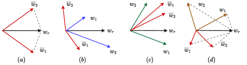
Figure 2: The vulnerabilities of similarity metrics in the two-dimensional plane. (a) shows the general similarity metrics’ vulnerabilities; (b)-(d) illustrate the vulnerabilities of $L_{2}$ norm, cosine similarity, and Euclidean distance, respectively.

Assume there are two benign local models $w_{1}$ and $w_{2}$ matching the lower and upper bounds of the similarity, respectively, two poisoned local models $\overline{w}_{1}$ and $\overline{w}_{2}$, and a reference model $w_{r}$ on the serve. The reference model is a hypothetical model that the defender uses to assist in model evaluation. In a more intuitive way, we demonstrate the vulnerabilities of similarity metrics in Figure 2. In Figure 2(a), we allow $\overline{w}_{1}$ and $\overline{w}_{2}$ share the same value of $L_{2}$ norm and have the same cosine similarity and Euclidean distance with $w_{r}$; however, they are in different directions. This means that local models that have the same similarity can be different. In Figure 2(b), poisoned local models $\overline{w}_{1}$ and $\overline{w}_{2}$ are evaluated as qualified but they are in different directions, and the same phenomena can be spotted in both in Figure 2(c) and Figure 2(d), revealing that multiple local models, which are significantly different, could be treated as qualified local models since their evaluated similarities are within the allowed range. In this way, the attackers can submit a well-crafted poisoned local model that satisfies the similarity requirements to undermine the global model.

4.2 Theoretical Analysis

Though Figure 2 illustrates the vulnerabilities of similarity metrics in FL, the mathematical principles behind the phenomenon are still unclear, which will be elaborated on next.

In general, when there is no attack, submissions from clients are supposed to have similar parameter values; however, when the FL system is under attack, the effective poisoned local models should have significantly different parameter values compared with the benign ones. Thus, we can summarize the vulnerabilities of similarity metrics below.

Definition 1.

(The “Curse” of Similarity) Given the benign local model $w_{i}$, the reference model $w_{r}$, and the similarity lower and upper bounds $s_{l}$ and $s_{u}$, the attacker can carefully craft a poisoned local model $\overline{w}_{i}$, so that $S(\overline{w}_{i},w_{r})\in[s_{l},s_{u}]$ while the parameter values in $w_{i}$ and $\overline{w}_{i}$ are significantly different.

To generate such a stealthy poisoned local model, a reasonable model for reference is required. Although $w_{r}$ is the optimal one, it is not accessible to the attacker. Recall the discussions about the capabilities and knowledge of attackers, they only know their own trained local models instantly and the global model in the previous round. Compared to the to-be-updated global model, the current local model $w_{i}$ is much closer to the reference model. So the attacker can use $w_{i}$ to approximate $w_{r}$ to generate the poisoned local model, i.e., $\overline{w}_{i}=\alpha_{i}\otimes w_{i}$ where $\otimes$ implies that $\overline{w}_{i,j}=\alpha_{i,j}w_{i,j}$ and $\alpha_{i}=(\alpha_{i,1},\cdots,\alpha_{i,j},\cdots,\alpha_{i,J})$ is the vector of scalars. However, how to ensure that there exists such an effective vector of scalars $\alpha_{i}$ remains another challenge. We provide the following theorem regarding this problem.

Theorem 1.

There exists at least one combination of scalars in $\alpha_{i}$ for local model $w_{i}$, $\forall\alpha_{i,j}>0,\exists\alpha_{i,j}\neq 1$, so that the attacker can generate a stealthy poisoned local model $\overline{w}_{i}$ based on $w_{i}$, i.e., $\overline{w}_{i}=\alpha_{i}\otimes w_{i}$.

The detailed proof is shown in Appendix A.1. With the above theorem, the attacker only needs to find such a vector to launch the attack. As for the method of obtaining $\alpha_{i}$, it will be detailed in Section 5.

From the above analysis, we know the deficiencies of the similarity metrics and the evidence for the existence of such deficiencies from a general perspective. However, the reasons for the prevalence of these defects in FL have not been explained. The main reason is that local models in FL usually have high dimensionality, and the similarity calculation considers the model as a whole but does not measure the value of each parameter, leaving room for attackers to design suitable scalars for different parameters to satisfy the similarity requirements. Besides, a given similarity requirement is usually not effective in detecting all aspects of the model. In particular, it is difficult for a single metric to measure both direction and magnitude. Although some defenses adopt multiple similarity metrics to evaluate the models, such as FLTrust and FLAME, we can still devise optimal attack strategies by transferring the attacks into optimization problems (see Section 5.2.1).

4.3 Manipulating Similarity in FL

Since we use the local model $w_{i}$ to approximate the reference model $w_{r}$, we can let $S(\overline{w}_{i},w_{i})$ as the approximate similarity of the poisoned local model $S(\overline{w}_{i},w_{r})$ during evaluation, which is denoted as $\overline{s}_{i}$. As an attacker, once the similarity metrics used by the defender are known, a poisoned local model can be generated based on $w_{i}$, which needs to satisfy the similarity requirements, i.e., the evaluated similarity $\overline{s}_{i}$ needs to be in the range of $[s_{l},s_{u}]$. Please note that such a range is only for the convenience of expression, it does not mean that all the defenses have strict upper and lower bounds of similarity, and the specific similarity requirements should be determined by analyzing different defenses. In general, the closer $\overline{s}_{i}$ is to the upper limit of its theoretical value, the more similar $\overline{w}_{i}$ is to $w_{r}$ and the less likely to eliminate $\overline{w}_{i}$. Thus, we can allow the attacker to maximize $\overline{s}_{i}$ in practice.

Note: Though the attacker can generate a stealthy poisoned local model, the attacking effectiveness cannot be guaranteed. Therefore, we have to explore maximizing the attack performance of such a poisoned local model generated based on the similarity metrics’ vulnerabilities, which will be introduced in the next section.

5 Faker: “Similar” but Harmful

We present a novel and effective model poisoning attack coined Faker by exploiting the deficiencies of similarity metrics to undermine FL. The core idea of Faker is to find an effective vector of scalars, i.e., $\alpha_{i}$, for the attacker to generate the poisoned local model $\overline{w}_{i}$ based on $w_{i}$. Specifically, Faker enables $\overline{w}_{i}$ to pass the detection of similarity-based defenses while maximizing its negative impacts on the global model. To generate such a poisoned local model, the attacker needs to ensure that the model will be recognized as “similar” but significantly different from the benign model in parameter values. Next, we introduce how Faker achieves both goals and formulate the general model of Faker. The illustration of Faker for a single device is in Figure 3. Note that Faker is designed for a single malicious client, meaning that cooperation among multiple attackers is not required, while we also provide strategies for the cooperation case in Section 5.4.

5.1 Model Formulation

As we have discussed in Section 4, the attacker uses the benign local model $w_{i}$ as an approximation to the unknown reference model $w_{r}$, and in order to avoid the bias caused by such approximation, the attacker can maximize the similarity between the generated poisoned local model and the benign local model, i.e., $\overline{s}_{i}$. If there is only one similarity metric being applied, we only need to calculate the similarity of $\overline{w}_{i}$ directly by $\overline{s}_{i}=S(\overline{w}_{i},w_{i})$; otherwise, we can multiply the calculated multiple similarities. For example, the similarity of $\overline{w}_{i}$ is $\overline{s}_{i}=C(\overline{w}_{i},w_{i})\frac{L(\overline{w}_{i})}{L(w_{i})}$ when FLTrust is applied and $\overline{s}_{i}=E(\overline{w}_{i},w_{i})$ when Krum is adopted. The reason for multiplying these similarities is that multiplied result is more convenient as an optimization objective than maximizing them separately. In this way, the first goal of Faker, i.e., generating “similar” poisoned local models, can be satisfied by maximizing $\overline{s}_{i}$. Since $\overline{w}_{i}=\alpha_{i}\otimes w_{i}$, we know that $\overline{s}_{i}=S(\overline{w}_{i},w_{i})$ is a function of the scalars in $\alpha_{i}$.

Intuitively, if two models are not the same, their parameters are different; and if we want to make the two models even more distinct, we can enlarge the difference in their parameters. We use the absolute value of the difference of the parameter values to represent the difference of the parameters, i.e., $\overline{\delta}_{i,j}=|\overline{w}_{i,j}-w_{i,j}|=|w_{i,j}(\alpha_{i,j}-1)|$. Thus, the difference between $\overline{w}_{i}$ and $w_{i}$ can be written as $\overline{\delta}_{i}=\sum_{j=1}^{J}{\overline{\delta}_{i,j}}=\sum_{j=1}^{J}|w_{i,j}(\alpha_{i,j}-1)|$. To achieve another goal of the attacker, which is to have significant differences between the submitted poisoned model and the benign one, we need to maximize $\overline{\delta}_{i}$. Since $w_{i,j}$ is a constant and $\alpha_{i,j}$ is positive, we allow $\overline{\delta}_{i}\approx\sum_{j=1}^{J}\alpha_{i,j}$ to serve as another maximization objective for the attacker to simplify the computation.

According to the above analysis, the attacker has to maximize both $\overline{s}_{i}$ and $\overline{\delta}_{i}$ by optimizing the scalars in $\alpha_{i}$ simultaneously. To further simplify the optimization problem, we let $f(\alpha_{i})=\overline{s}_{i}\overline{\delta}_{i}$ represent the overall optimization objective. Thus, we can propose a general model of Faker for a single attacker $i$ as follows:

P0: $$\mathop{\arg\max}_{\alpha_{i}}\quad f(\alpha_{i})$$

$$s.t.\quad C1:~{}\overline{s}_{i}\in[s_{l},s_{u}],$$

$$C2:~{}\forall\alpha_{i,j}>0,\exists\alpha_{i,j}\neq 1,$$

where $f(\alpha_{i})=\overline{s}_{i}\overline{\delta}_{i}$ is the optimization objective function; $\overline{s}_{i}$ and $\overline{\delta}_{i}$ are the similarity and difference of poisoned local model $\overline{w}_{i}$, respectively; the scalars $\alpha_{i,1},\cdots,\alpha_{i,j},\cdots,\alpha_{i,J}$ are the optimization variables, and there are $J$ variables in total; $C1$ is the similarity requirement of the adopted defense, which means that the poisoned local model should satisfy the requirement to avoid being detected; and $C2$ is the feasible domain of $\alpha_{i,j}$. Since different defenses adopt different similarity metrics and have different rules, the attacker has to adapt P0 to specific defenses. The two main steps for the attacker to launch Faker are to formulate $f(\alpha_{i})$ and determine the bounds of $\overline{s}_{i}$, which will be detailed when we design Faker against different defenses in Section 5.2.

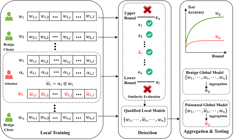
Figure 3: The illustration of Faker for the single attacker. After training, the attacker obtains local model $w_{i}$, and it launches the attack by calculating the scalars and generating poisoned local model $\overline{w}_{i}$ according to Algorithm 1; when the submissions are evaluated by similarity-based defenses, the poisoned local model generated by Faker can avoid being detected and the poisoned global model will be significantly different from the benign one, degrading the test accuracy.

P0 is a non-linear optimization problem with inequity constraints and $J$ variables in total, and thus solving it is nontrivial. To enable a quick decision for the attacker, we intend to avoid using computationally intensive solutions, such as heuristic algorithms, distributed optimization algorithms, and reinforcement learning based algorithms. We propose a simple yet effective strategy to reduce the complexity of solving P0 by choosing only one scalar, e.g., $\alpha_{i,j}$, as a variable, while any scalar except $\alpha_{i,j}$ in $\alpha_{i}$ is set as a constant from a well designed feasible domain. Note that we need to set values for $J-1$ scalars except $\alpha_{i,j}$ in $\alpha_{i}$, and for convenience of expression, we use $\alpha_{i,-j}$ and $w_{i,-j}$ to denote any such scalar and the corresponding parameter in $w_{i}$, respectively.

Algorithm 1 Faker

0:  The local model $w_{i}=(w_{i,1},\cdots,w_{i,j},\cdots,w_{i,J})$ and the adopted defense

0:  The generated poisoned local model $\overline{w}_{i}$The malicious client $i$ executes:

1:  $\alpha_{i}=(\alpha_{i,1},\cdots,\alpha_{i,j},\cdots,\alpha_{i,J}),\forall\alpha_{i,j}>0,\exists\alpha_{i,j}\neq 1\leftarrow$ Initiates $J$ scalars as the unknown variables

2:  $\overline{s}_{i}$, $\overline{\delta}_{i}$ $\leftarrow$ Expresses the similarity and difference of the poisoned local model $\overline{w}_{i}$ by $\alpha_{i,j}$ and $w_{i,j}$

3:  $s_{l},s_{u}\leftarrow$ Obtains the lower and upper bounds of similarity requirement by analyzing the adopted defense

4:  Maximizes the objective function $f(\alpha_{i})=\overline{s}_{i}\overline{\delta}_{i}$ that subjects to $\overline{s}_{i}\in[s_{l},s_{u}]$ by optimizing $\alpha_{i,j}$

5:  $\alpha_{i}\leftarrow$ Solves the above optimization problem

6:  return  $\overline{w}_{i}=\alpha_{i}\otimes w_{i}=(\overline{w}_{i,1},\cdots,\overline{w}_{i,j},\cdots,\overline{w}_{i,J})$

We summarize Faker as Algorithm 1. Specifically, when launching Faker, an attacker only needs its own local model $w_{i}$ and the defense adopted by the defender. Sometimes some other information is needed, such as the global model $w_{g}$ from the previous round when attacking Krum. The goal of the attacker is to find a $J$-dimensional vector $\alpha_{i}$ to generate a poisoned local model $\overline{w}_{i}$. All scalars in $\alpha_{i}$ must be positive and cannot both have value 1 (Line 1). Next, the attacker needs to express the similarity $\overline{s}_{i}$ and difference $\overline{\delta}_{i}$ of $\overline{w}_{i}$ using $\alpha_{i,j}$ and $w_{i,j}$ respectively (Line 2). The lower and upper bounds of the similarity requirement, i.e., $s_{l}$ and $s_{u}$, can be deduced from the adopted defense (Line 3). Then, the attacker formulates an optimization problem with maximizing the objective function $f(\alpha_{i})=\overline{s}_{i}\overline{\delta}_{i}$ that subjects to $\overline{s}_{i}\in[s_{l},s_{u}]$ by optimizing all the scalars in $\alpha_{i}$. As for the solutions to the formulated optimization problem, we will detail them in Section 5.2 according to different defenses (Line 5). In the end, the attacker can generate $\overline{w}_{i}$ by $\overline{w}_{i}=\alpha_{i}\otimes w_{i}$ and submit it to the server (Line 6). The complexity analysis is presented in Section 5.3.

5.2 Faker Against Similarity-based Defenses

Due to limited space, we cannot present detailed designs for attacking all similarity-based defenses. We choose three representative defenses, i.e., FLTrust, Krum, and norm-clipping, to illustrate how to adjust P0 for different defenses. Since these three defenses cover the three similarity metrics mentioned earlier, adapting Faker to attack other defenses can also refer to the following designs. Appendix B.1 provides the detailed designs of Faker against three other benchmark defenses, i.e., FLAME, DiverseFL, and ShieldFL.

5.2.1 Faker Against FLTrust

FLTrust applies both cosine similarity and $L_{2}$ norm to protect FL, and we can calculate the poisoned local model’s similarity as $\overline{s}_{i}=C(\overline{w}_{i},w_{i})\frac{L(\overline{w}_{i})}{L(w_{i})}$, and we can express it with $\alpha_{i,j}$ and $w_{i,j}$ as $\overline{s}_{i}=\frac{\sum_{j=1}^{J}w^{2}_{i,j}\alpha_{i,j}}{\sum_{j=1}^{J}w^{2}_{i,j}\alpha_{i,j}^{2}}$. In this way, the objective function can be written as:

$$f(\alpha_{i})=\frac{\sum_{j=1}^{J}w^{2}_{i,j}\alpha_{i,j}\sum_{j=1}^{J}\alpha_{i,j}}{\sum_{j=1}^{J}w^{2}_{i,j}\alpha_{i,j}^{2}}.$$

Then, we can transform Faker against FLTrust into the following optimization problem:

$$\textbf{P1}: \mathop{\arg\max}_{\alpha_{i}}\quad f(\alpha_{i}),$$

s.t. $$\textit{C1}:C(\overline{w}_{i},w_{i})>0,$$

$$\textit{C2}:~{}\forall\alpha_{i,j}>0,\exists\alpha_{i,j}\neq 1,$$

where $C1$ ensures the corrupted local model will not be discarded by FLTrust. By solving P1, we have the following theorem. The detailed proofs are in Appendix A.2.

Theorem 2.

(Faker Against FLTrust) Setting $\alpha_{i,-j}$ with random positive values, we can get the approximate optimal value of $\alpha_{i,j}$ by

$$\alpha_{i,j}^{*} =\frac{w^{2}_{i,j}(\beta-\lambda\gamma)+[w^{2}_{i,j}(\lambda^{2}+w^{2}_{i,j}\beta)(w^{2}_{i,j}\gamma^{2}+\beta)]^{\frac{1}{2}}}{w^{2}_{i,j}(\lambda+w_{i,j}^{2}\gamma)},\$$

where $\lambda=\sum_{-j=1}^{J-1}\alpha_{i,-j}w^{2}_{i,-j}$, $\beta=\sum_{-j=1}^{J-1}\alpha_{i,-j}^{2}w^{2}_{i,-j}$, and $\gamma=\sum_{-j=1}^{J-1}\alpha_{i,-j}$.

5.2.2 Faker Against Krum

In Krum, only one local model will be selected as the global model in each round. Thus, to attack Krum, we must ensure that $\overline{w}_{i}$ will be selected. The similarity of $\overline{w}_{i}$ is $\overline{s}_{i}=E(\overline{w}_{i},w_{i})$, and the objective function is:

$$f(\alpha_{i})=[\sum^{J}_{j=1}(\alpha_{i,j}w_{i,j}-w_{i,j})^{2}]^{\frac{1}{2}}\sum_{j=1}^{J}\alpha_{i,j}.$$

To ensure that $\overline{w}_{i}$ can be selected, we need to enable it to have the minimum sum of Euclidean distances from the other models. We can satisfy this requirement by finding the upper bound of the distance of $\overline{w}_{i}$ between any other benign model. Such a distance can be approximately represented by the distance of $\overline{w}_{i}$ and $w_{i}$, i.e., $E(\overline{w}_{i},w_{i})$. As a single attacker, it only knows the global model $w_{g}$ besides its trained local model $w_{i}$ in this round. In this way, we can use the distance between the global model $w_{g}$ and the local model $w_{i}$, i.e., $E(w_{g},w_{i})$, as the approximated upper bound of $E(\overline{w}_{i},w_{i})$. Thus, we have $E(\overline{w}_{i},w_{i})<E(w_{g},w_{i})$. Then, we formulate Faker against Krum as below:

$$\textbf{P2}: \mathop{\arg\max}_{\alpha_{i}}\quad f(\alpha_{i})$$

$$\textit{s.t.}:\quad~{} \textit{C1}:E(\overline{w}_{i},w_{i})<E(w_{g},w_{i}),$$

$$\textit{C2}:~{}\forall\alpha_{i,j}>0,\exists\alpha_{i,j}\neq 1,$$

where $C1$ ensures that $\overline{w}_{i}$ can be selected; and $C2$ is the domain of $\alpha_{i,j}$. By solving this optimization problem, we have the following theorem.

Theorem 3.

(Faker Against Krum) Setting $\alpha_{i,-j}$ with any value that satisfies $0<\alpha_{i,-j}\leq 1+\frac{E(w_{g},w_{i})}{[(J-1)\max(w_{i,-j})]^{\frac{1}{2}}}$, then the approximate value of $\alpha_{i,j}$ is calculated by

$$0<\alpha_{i,j}<\frac{1}{w_{i,t}}(w_{i,j}+\Omega),$$

where $\Omega=[w_{i,j}(\sum_{-j=1}^{J-1}((2\alpha_{i,-j}-\alpha_{i,-j}^{2}-1)w_{i,-j})+{E(w_{g},w_{i})}^{2})]^{\frac{1}{2}}$.

Please see Appendix A.3 for proofs. Note that the inequality above only provides a lower bound and an upper bound of $\alpha_{i,j}$, and since $f(\alpha_{i})$ is a monotonically increasing function when $\alpha_{i,j}>0$, we can take a value slightly smaller than upper bound as the optimal value $\alpha_{i,j}^{*}$.

5.2.3 Faker Against Norm-clipping

Since norm-clipping adopts $L_{2}$ norm to measure the reliability of local models, the optimization objective function becomes:

$$f(\alpha_{i})=[\sum_{j=1}^{J}\alpha_{i,j}^{2}w_{i,j}^{2}]^{\frac{1}{2}}\sum_{j=1}^{J}\alpha_{i,j}.$$

Norm-clipping requires that the $L_{2}$ norms of local models are less than the upper bound and treats local models failing the requirement as malicious models for removal. We can use the $L_{2}$ norm of the local model $w_{i}$ as the upper bound. In this way, we have $L(\overline{w}_{i})\leq L(w_{i})$.

Then, we can formulate Faker against norm-clipping as:

$$\textbf{P3}: \mathop{\arg\max}_{\alpha_{i}}\quad f(\alpha_{i})$$

$$\textit{s.t.}:\quad~{} \textit{C1}:L(\overline{w}_{i})\leq L(w_{i}),$$

$$\textit{C2}:~{}\forall\alpha_{i,j}>0,\exists\alpha_{i,j}\neq 1,$$

where $C1$ ensures that the poisoned local models will not be discarded by norm-clipping and $C2$ is the domain. We can solve P3 and summarize it into the following theorem. Please refer to Appendix A.4 for proofs.

Theorem 4.

(Faker Against Norm-clipping) Let $\alpha_{i,-j}$ be any number which satisfies $0<\alpha_{i,-j}\leq[\frac{L(w_{i})^{2}}{(J-1)\max(w_{i,-j})}]^{\frac{1}{2}}$, then the approximate optimal value of $\alpha_{i,j}$ is calculated by

$$\alpha_{i,j}^{*}=\big{(}\frac{1}{w_{i,j}}\big{[}\sum_{-j=1}^{J-1}(-\alpha^{2}_{i,-j}w_{i,-j})+{L(w_{i})}^{2}\big{]}\big{)}^{\frac{1}{2}}.$$

Note: Once the malicious client $i$ calculates all the scalars in $\alpha_{i}$, it can directly generate the poisoned local model by multiplying scalars and parameters, i.e., $\overline{w}_{i}=\alpha_{i}\otimes w_{i}$, and then submit the poisoned local model to the server.

5.3 Complexity Reduction

Following our previous analysis, Faker needs to determine the values of the $J$ scalars in $\alpha_{i}$. Even though we adopt the method that sets values for $J-1$ in a well-defined domain and remains only one variable to reduce the complexity, the computational cost is still significant when $J$ is large with the worst-case time complexity $\mathcal{O}(J)$. To further simplify the computation of $\alpha_{i}$, we can divide the scalars into $T\ll J$ groups and allow the scalars in the same group to share the same value, thus the time complexity can be reduced to $\mathcal{O}(T)$. As for the dividing method, one straightforward way is to treat the parameters in the same layer of deep learning models as in the same group.

5.4 Attacking Mode

In most cases, it is difficult to attack an FL system by controlling multiple local clients at the same time. Unlike most existing attacks, we advocate that a single attacker launches an attack independently without requiring cooperation among multiple clients. In this way, Faker only needs to generate poisoned local models based on the attacker’s own local model. In addition, we also provide strategies for Faker in the case of cooperation among attackers. Specifically, attackers are allowed to communicate with each other the local models used to get an intermediate global model $w_{g}$ to approximate the reference model $w_{r}$ on the defender. Besides, for attacking Krum, we let attacker $i$ send its obtained poisoned local model $\overline{w}_{i}$ to the other $m-1$ attackers, who also submit $\overline{w}_{i}$ to the server; in this way, the upper bound of similarity should be adjusted as $E(\overline{w}_{i},w_{i})<\frac{n-m-1}{n-2m-1}E(w_{g},w_{i})$. This paper only provides a preliminary exploration of the attacking mode and more in-depth research is needed in the future.

6 Evaluation of Faker

In this section, we verify the threat of Faker to FL performance through extensive experiments. We describe the experimental settings in detail and then present results with corresponding discussions. The experiments are conducted using Python 3.10, TensorFlow 2.8, and PyTorch 2.0 running on a desktop with an NVIDIA GeForce RTX 3080 GPU.

6.1 Experimental Settings

Datasets. Experimental results presented below are mainly based on MNIST [28], Fashion MNIST (FMNIST) [45], and CIFAR-10 [24]. MNIST is a handwritten digit database that contains 70000 images for 0 to 9 with the size of 28 $\times$ 28. We split the dataset into training and test data with 60000 and 10000 images, respectively. FMNIST is an article image dataset that contains 60000 images as training data and 10000 images as test data. Each sample in FMNIST is a 28 $\times$ 28 grayscale image with a label from 0 to 9. CIFAR-10 is a 32 $\times$ 32 color image dataset with 6000 images in each class and 10 classes in total, including 50000 images as training images and 10000 test images.

Data Distribution. To study the effect of data distribution on adversarial attacks, we obtain the IID and Non-IID datasets by the following method: since MNIST, FMNIST, and CIFAR-10 have 10 classes, we can divide the training data by controlling the number of classes $c\in[1,10]$ that each client can obtain. We consider such a division as IID when $c=10$, and we obtain the non-IID data by setting $c<10$.

Deep Learning Models. We use an MLP model to train MNIST data, which contains a Flatten layer, two Dense layers, and one Dropout layer. As for FMNIST, a CNN model with two Convolution2D layers, one MaxPooling2D layer, two Dropout layers, two Dense layers, and one Flatten layer is designed. Besides, we design a CNN model with three Convolution2D layers, two Maxpooling2D layers, two Dense layers, and one Flatten layer for CIFAR-10. At the beginning of local training, the parameters are randomly generated. During training, we adopt Adam with the default hyperparameter settings in PyTorch as the optimizer of the deep learning models. To maintain consistency, in our experiments, local models are converted to vectors when evaluated by defenses.

Benchmark Defenses. In experiments, seven aggregation methods, i.e., FedAvg (FA), Krum (KM), norm-clipping (NC), FLTrust (FT), FLAME (FM), DiverseFL (DF), and ShieldFL (SF), are applied to defend against model poisoning attacks; and we use NC, FM, and DF to defend against backdoor attack; and FoolsGod is implemented to detect Sybil attacks. As for FLTrust, DiverseFL, and ShieldFL, the clean data set containing 100 examples is randomly selected from testing data. As for norm-clipping, besides its upper bound, we also provide a lower bound, which is four-fifths of the upper bound to prevent the attackers from submitting poisoned local models with very small parameters. FedAvg cannot tolerate adversarial attacks, so we use its results in the case of non-attack (N/A) to compare with the results of other defenses.

Benchmark Attacks. We apply LA and MB as the benchmark model poisoning attacks. We follow the basic ideas of LA and MB and design corresponding attacks against the benchmark defenses. We set $10^{-5}$ as the threshold for both LA and MB. For Faker, we divide the vector of scalars $\alpha_{i}$ into two parts (i.e., $T=2$) to reduce the time consumption of generating poisoned local models. As for the dividing methods, we allow Faker to choose one layer (e.g., the output layer) as the first group and the rest of the layers as the second group, and the shared scalar for the first group is variable.

Federated Learning Framework. We consider one FL system with 100 clients. In each round, we assume that the server will select all local clients to participate in the training and that each client has sufficient computational, communication, and storage resources to submit a local model in time.

Performance Measurements. We use the error rate (ER), success rate (SR), and time consumption (TC) of launching the attack to measure the attacking performance of Faker on the model poisoning and Sybil attacks. As for the backdoor attack, we adopt the main task accuracy (MA), targeted task accuracy (TA), and TC as the evaluation metrics. The above measurements will be detailed during the evaluation.

Attacking Mode. For Faker, if not specifically stated, the experiments are conducted with a non-cooperative attack strategy, i.e., the attackers would not be aware of each other. As for other benchmark attacks, attackers are allowed to collude with each other; however, when measuring the time cost it will be the same as Faker, only measuring the time consumption to launch the attack by a single device to ensure a fair comparison.

6.2 Experimental Results

We present partial experimental results in this section, and readers can refer to Appendix B.3 for extra results.

Table 3: Error rates of IID data ($c=10$) with $n=100$ and $m=20$. When there is no attack, the error rates of FA for MNIST, FMNIST, and CIFAR-10 are 0.06, 0.17, and 0.40.

Dataset	Attack	KM	NC	FT	FM	DF	SF
MNIST	N/A	0.14	0.06	0.07	0.07	0.06	0.07
	LA	0.16	0.07	0.04	0.06	0.06	0.06
	MB	0.16	0.07	0.04	0.06	0.06	0.06
	Faker	0.18	0.17	0.12	0.22	0.56	0.90
FMNIST	N/A	0.22	0.17	0.15	0.19	0.18	0.15
	LA	0.22	0.18	0.18	0.18	0.20	0.17
	MB	0.21	0.19	0.17	0.16	0.20	0.17
	Faker	0.23	0.23	0.23	0.77	0.40	0.90
CIFAR-10	N/A	0.49	0.40	0.41	0.46	0.48	0.48
	LA	0.52	0.43	0.75	0.46	0.48	0.49
	MB	0.51	0.41	0.74	0.46	0.50	0.49
	Faker	0.64	0.55	0.77	0.48	0.65	0.68

Table 4: Error rates of non-IID data ($c=2$) with $n=100$ and $m=20$. The error rates of FA for the two datasets are 0.17 and 0.20 when there is no attack.

Dataset	Attack	KM	NC	FT	FM	DF	SF
MNIST	N/A	0.89	0.17	0.12	0.15	0.20	0.16
	LA	0.90	0.33	0.30	0.15	0.20	0.90
	MB	0.90	0.19	0.16	0.15	0.17	0.90
	Faker	0.90	0.80	0.34	0.50	0.78	0.90
FMNIST	N/A	0.81	0.20	0.18	0.19	0.20	0.90
	LA	0.85	0.20	0.72	0.19	0.20	0.90
	MB	0.86	0.20	0.80	0.19	0.20	0.90
	Faker	0.90	0.73	0.82	0.90	0.48	0.90

Impacts of Data Distribution on Faker. By setting $c=10$ and $c=2$ to get IID and non-IID data, we evaluate Faker with different data distributions. The evaluation of IID data is based on MNIST, FMNIST, and CIFAR-10, and the evaluation of non-IID is based on MNIST and FMNIST. The results on CIFAR-10 are not presented when $c=2$ since they can not even converge when there is no attack. We set $m=20$ and use test error rates to measure the performance of attacks. The results are shown in Table 3 and Table 4. Overall, we know that Faker outperforms LA and MB in both IID and non-IID situations among all the datasets and defenses. Specifically, for MNIST, when $c=10$, both LA and MB do not degrade the performances of FLTrust, FLAME, DiverseFL, and ShieldFL, and they only decrease a little when attacking Krum and norm-clipping, but Faker can undermine all these defenses; for FMNIST and CIFAR-10, the impacts of Faker on these defenses are more significant. When $c=2$, both LA and MB degrade the accuracy of the defenses except FLAME, and Faker greatly undermines all the defenses. Compared with LA and MB, Faker is more powerful in attacking and more compatible with IID and non-IID data.

Table 5: Error rates of different numbers of malicious clients when $c=5$ and $n=100$. The error rates of FA for the three datasets are 0.09, 0.17, and 0.52 when no attack.

$m/n$	Dataset	Attack	KM	NC	FT	FM	DF	SF
0%	MNIST	N/A	0.48	0.11	0.09	0.10	0.09	0.09
	FMNIST	N/A	0.40	0.19	0.17	0.18	0.19	0.54
	CIFAR-10	N/A	0.64	0.52	0.55	0.58	0.52	0.56
1%	MNIST	LA	0.50	0.11	0.06	0.10	0.10	0.10
		MB	0.49	0.10	0.06	0.10	0.06	0.10
		Faker	0.54	0.12	0.10	0.10	0.13	0.90
	FMNIST	LA	0.45	0.19	0.17	0.18	0.19	0.56
		MB	0.36	0.19	0.16	0.18	0.18	0.55
		Faker	0.50	0.19	0.19	0.20	0.23	0.90
	CIFAR-10	LA	0.65	0.55	0.57	0.58	0.55	0.90
		MB	0.62	0.55	0.55	0.59	0.55	0.61
		Faker	0.66	0.60	0.58	0.63	0.61	0.90
5%	MNIST	LA	0.54	0.11	0.06	0.10	0.10	0.24
		MB	0.52	0.10	0.06	0.10	0.10	0.16
		Faker	0.60	0.14	0.41	0.11	0.36	0.90
	FMNIST	LA	0.34	0.20	0.18	0.18	0.20	0.57
		MB	0.46	0.19	0.17	0.18	0.18	0.59
		Faker	0.53	0.20	0.21	0.24	0.37	0.90
	CIFAR-10	LA	0.65	0.55	0.65	0.76	0.55	0.90
		MB	0.62	0.52	0.64	0.78	0.55	0.77
		Faker	0.68	0.80	0.67	0.83	0.79	0.90
10%	MNIST	LA	0.60	0.10	0.09	0.10	0.10	0.78
		MB	0.57	0.11	0.08	0.10	0.10	0.67
		Faker	0.64	0.16	0.90	0.20	0.59	0.90
	FMNIST	LA	0.50	0.11	0.23	0.18	0.21	0.85
		MB	0.48	0.11	0.11	0.18	0.19	0.79
		Faker	0.61	0.24	0.55	0.30	0.55	0.90
	CIFAR-10	LA	0.66	0.55	0.77	0.82	0.55	0.90
		MB	0.63	0.53	0.76	0.80	0.55	0.90
		Faker	0.70	0.90	0.78	0.90	0.90	0.90
20%	MNIST	LA	0.61	0.11	0.08	0.10	0.10	0.90
		MB	0.60	0.11	0.06	0.10	0.10	0.90
		Faker	0.66	0.18	0.90	0.43	0.66	0.90
	FMNIST	LA	0.90	0.21	0.30	0.32	0.21	0.90
		MB	0.59	0.21	0.25	0.30	0.18	0.90
		Faker	0.90	0.34	0.60	0.90	0.69	0.90
	CIFAR-10	LA	0.68	0.55	0.83	0.90	0.55	0.90
		MB	0.64	0.54	0.82	0.90	0.55	0.90
		Faker	0.76	0.90	0.85	0.90	0.90	0.90
50%	MNIST	LA	0.90	0.11	0.23	0.40	0.10	0.90
		MB	0.59	0.11	0.11	0.54	0.10	0.90
		Faker	0.90	0.34	0.90	0.60	0.81	0.90
	FMNIST	LA	0.90	0.21	0.65	0.60	0.21	0.90
		MB	0.90	0.21	0.63	0.70	0.19	0.90
		Faker	0.90	0.39	0.72	0.90	0.90	0.90
	CIFAR-10	LA	0.90	0.55	0.90	0.90	0.55	0.90
		MB	0.90	0.57	0.90	0.90	0.55	0.90
		Faker	0.90	0.90	0.90	0.90	0.90	0.90

Impacts of Malicious Clients’ Number on Faker. Intuitively, with more malicious clients, the impacts of the model poisoning attacks will be more significant. To support this idea, we set $n=100$ and vary the number of malicious clients $m$; and $m/n$ represents the proportion of malicious clients to all the clients. To simulate the practical application scenario of FL, we set $c=5$ to get the non-IID data. The experimental results are presented in Table 5. From the results, Faker successfully achieves the reduction in model performance regardless of the variation in $m/n$, datasets, and defenses and outperforms both LA and MB. Even when there is only one malicious client, Faker can still undermine similarity-based defenses, while the other two model poisoning attacks have poor performance. It is worth noting that LA and MB have almost no effect on norm-clipping because LA and MB can only meet the requirements of norm-clipping by maintaining or reducing the magnitude of the local model. With the upper and lower bounds we have set for norm-clipping, it is more difficult for LA and MB to generate the required poisoned models to attack norm-clipping. Since Faker only needs to generate poisoned models that meet the requirement of the upper bound according to the formula when attacking norm-clipping, the attack is not affected by the lower bound. From the results of the experiments, we can argue that the more malicious clients we have, the more successful the Faker attack will be. Furthermore, Faker can effectively perform well with few malicious clients so as to attack industrial FL [39].

Single Round Attack. In the previous experiments, we assume that the attackers launch attacks in each round, but in reality, smart attackers often launch attacks when the global model is converging in order to hide themselves and reduce the model performance at the same time. In our experiments, we test Faker’s performance in launching a single attack in one round when the local loss is small. The results in Table 6 indicate that Faker outperforms the benchmark attacks and can still undermine the global model by attacking only once.

Table 6: Error rates when only attack once with $c=5$, $n=100$, and $m=20$. The error rates of FA for the three datasets are 0.09, 0.17, and 0.52 when no attack.

Dataset	Attack	KM	NC	FT	FM	DF	SF
MNIST	N/A	0.48	0.11	0.09	0.10	0.09	0.09
	LA	0.48	0.11	0.09	0.10	0.12	0.12
	MB	0.48	0.11	0.09	0.10	0.11	0.10
	Faker	0.52	0.12	0.10	0.12	0.14	0.78
FMNIST	N/A	0.40	0.19	0.17	0.18	0.19	0.54
	LA	0.40	0.21	0.17	0.20	0.19	0.90
	MB	0.40	0.19	0.17	0.18	0.19	0.90
	Faker	0.54	0.26	0.20	0.34	0.30	0.90
CIFAR-10	N/A	0.64	0.52	0.55	0.58	0.52	0.56
	LA	0.64	0.52	0.55	0.60	0.52	0.90
	MB	0.64	0.52	0.55	0.59	0.52	0.90
	Faker	0.68	0.64	0.57	0.80	0.56	0.90

Success Rates of Faker. We first define success rates as the percentage of effective attack rounds to total training rounds. For each defense, the measurements of a successful attack will be different. Since FLTrust and FLAME use similarity evaluation results to filter out outliers, we define that the attacks toward them are successful if they accept all the poisoned submissions. As for Krum, the attack is successful if one of the poisoned local models is selected as the global model. In our experiments, norm-clipping and DiverseFL both have lower and upper bounds, so we define the attack as successful if no discarded poisoned submissions. As for ShieldFL, we define the attack as successful if the poisoned model is assigned a higher weight during aggregation. Our definition of a successful attack is strict in that if any poisoned model is rejected in any round, the attack is not considered successful in that round. We set $n=100$, $m=20$, and $c=5$, then train 100 rounds. From the experimental results presented in Table 7, we can see that Faker can always get a 100% success rate with different datasets and defenses. However, LA and MB can not always get high success rates, especially when attacking Krum and DiverseFL, because they generate poisoned local models in an iterative method which can not guarantee all the poisoned submissions can meet the requirements of defenses. Moreover, in Faker, we use rigorous mathematical analysis to derive the optimal attack strategies, ensuring defenses can accept all the poisoned local models.

Table 7: Evaluation of success rate of attack with $n=100$, $m=20$, and $c=5$ by running 100 rounds.

	MNIST			FMNIST			CIFAR-10
Defenses	LA	MB	Faker	LA	MB	Faker	LA	MB	Faker
KM	0.04	0.02	1.00	0.00	0.00	1.00	0.09	0.05	1.00
NC	0.94	0.89	1.00	0.87	0.85	1.00	0.73	0.66	1.00
FT	1.00	1.00	1.00	1.00	1.00	1.00	1.00	1.00	1.00
FM	0.00	0.00	1.00	0.45	0.37	1.00	1.00	1.00	1.00
DF	0.00	0.00	1.00	0.06	0.00	1.00	0.00	0.00	1.00
SF	1.00	1.00	1.00	1.00	1.00	1.00	1.00	1.00	1.00

Table 8: Evaluation of time consumption with $n=100$, $m=20$, and $c=5$. The time cost is measured in seconds.

	MNIST			FMNIST			CIFAR-10
Defenses	LA	MB	Faker	LA	MB	Faker	LA	MB	Faker
KM	5.812	5.064	0.827	40.632	39.115	6.234	7.254	7.143	4.242
NC	0.026	0.022	0.015	0.142	0.122	0.083	0.682	0.136	0.093
FT	0.089	0.070	0.015	0.129	0.124	0.016	0.069	0.067	0.030
FM	0.231	0.211	0.183	0.443	0.486	0.336	0.568	0.435	0.245
DF	0.258	0.374	0.214	0.474	0.264	0.173	1.322	0.353	0.225
SF	0.231	0.293	0.152	0.835	0.459	0.235	0.335	0.362	0.242

Time Consumption of Faker. Then, we explore the time cost of launching Faker by a single attacker, which is measured in seconds. By setting $n=100$, $m=20$, and $c=5$, we can directly get the running time of launching different attacks. According to results in Table 8, Faker is much more time efficient in launching attacks against similarity-based defenses with three datasets. Since our tests are conducted on a device with a GPU, all experimental values are within one minute, but for mobile devices that do not have high computing power, it would be time-consuming and impractical to launch LA and MB attacks when Krum is applied. Faker takes less time than the other attacks, even if attacking Krum.

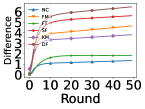
(a) MNIST.

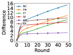
(b) FMNIST.

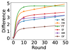
(c) CIFAR-10.

Figure 4: Evaluation of global model’s difference with $n=100$, $m=20$, and $c=5$.

Difference Between Benign and Poisoned Global Models. We randomly select two parameters from both poisoned and unpoisoned global models in each round to measure the difference caused by Faker. We set $n=100$, $m=20$, and $c=5$, and the experimental results are presented in Fig. 4. From the results, it can be seen that the difference due to the poisoned model generated by Faker is greater than 1 after multiple rounds. It is important to note that the parameters of the FL model are usually numbers with absolute values much smaller than 1. Therefore, we can conclude that the poisoned model is sufficient to cause the performance degradation of the global model.

Evaluation of Attacking Mode. We also evaluate Faker’s performance in different attack modes. The experimental results are shown in Table 9, which demonstrate that the cooperation mode outperforms the non-cooperation mode. However, the attack in non-cooperative mode is sufficient in terms of its effectiveness.

Table 9: Error rates of Faker in different attacking modes with $c=5$, $n=100$, and $m=20$, where “single” and “cooperation” refer to non-cooperation and cooperation modes, respectively.

Dataset	Mode	KM	NC	FT	FM	DF	SF
MNIST	cooperation	0.69	0.24	0.90	0.26	0.65	0.90
	single	0.64	0.16	0.90	0.20	0.59	0.90
FMNIST	cooperation	0.90	0.37	0.64	0.90	0.72	0.90
	single	0.90	0.34	0.60	0.90	0.69	0.90
CIFAR-10	cooperation	0.79	0.90	0.89	0.90	0.90	0.90
	single	0.76	0.90	0.85	0.90	0.90	0.90

Extending Faker to Other Attacks. Even though we focus on the untargeted model poisoning attacks in this work, we still provide the evaluation of Faker-based targeted backdoor attacks and Sybil attacks, and their detailed designs are shown in Appendix B.2. From Table 10, we can see that the backdoor attack based on Faker can better maintain the main task accuracy (MA) and decrease the targeted task accuracy (TA) with less time consumption compared to the benchmark attack. The results in Table 11 show that the Faker-based Sybil attack can bypass the detection of FoolsGold [14] and has better performance in decreasing the accuracy, success rate, and time cost than the benchmark adopted in [14]. The above experimental results indicate that Faker can be well extended to other adversarial attacks, further illustrating the threats of similarity metrics’ vulnerabilities.

Table 10: Evaluation of Faker-based backdoor attack. The performance is measured by main task accuracy (MA), targeted task accuracy (TA), and time cost (TC) of attack. NC w. Faker means using Faker to attack NC. “-” implies not applicable. We set $n=100$, $m=20$, and $c=5$.

	MNIST			FMNIST			CIFAR-10
Defenses	MA	TA	TC	MA	TA	TC	MA	TA	TC
NC w. N/A	0.97	0.99	-	0.82	0.64	-	0.57	0.45	-
NC w. C&S	0.86	0.61	0.03	0.70	0.45	0.09	0.43	0.25	0.13
NC w. Faker	0.93	0.52	0.01	0.73	0.32	0.08	0.46	0.23	0.09
FM w. N/A	0.97	0.99	-	0.82	0.67	-	0.57	0.44	-
FM w. C&S	0.92	0.50	0.03	0.72	0.26	0.09	0. 49	0.28	0.18
FM w. Faker	0.94	0.48	0.02	0.74	0.23	0.07	0. 51	0.26	0.11
DF w. N/A	0.97	0.99	-	0.82	0.65	-	0.23	0.21	-
DF w. C&S	0.92	0.63	0.25	0.68	0.35	0.32	0.47	0.23	0.43
DF w. Faker	0.95	0.56	0.22	0.71	0.32	0.24	0.49	0.11	0.32

Table 11: Evaluation of Faker-based Sybil attack. The performance is measured by error rate (ER), success rate (SR), and time cost (TC) of attack. FoolsGold w. Faker means using Faker to attack FoolsGold. “-” implies not applicable. We set $n=100$, $m=20$, and $c=5$.

	MNIST			FMNIST			CIFAR-10
Defenses	ER	SR	TC	ER	SR	TC	ER	SR	TC
FoolsGold w. N/A	0.10	-	-	0.18	-	-	0.52	-	-
FoolsGold w. [14]	0.10	0.00	0.12	0.18	0.00	0.23	0.52	0.00	0.56
FoolsGold w. Faker	0.63	1.00	0.01	0.49	1.00	0.01	0.90	1.00	0.03

Impacts of $T$ on Faker’s Performance. We explore the effect of $T$ on Faker’s performance by varying its value. The results are presented in Table 12 and Table 13. We can see that increasing the value of $T$ will not greatly improve the overall attack performance, but it will significantly increase the time cost required to launch the attack. Therefore, we suggest that an attacker can choose a smaller $T$ in practice to achieve the expected attacking goal while reducing the time consumption.

Table 12: Error rates of different values of $T$ with $n=100$, $m=20$, and $c=5$.

	MNIST			FMNIST			CIFAR-10
Defenses	T=2	T=J/2	T=J	T=2	T=J/2	T=J	T=2	T=J/2	T=J
KM	0.66	0.66	0.67	0.90	0.90	0.90	0.76	0.77	0.77
NC	0.18	0.18	0.19	0.34	0.35	0.35	0.90	0.90	0.90
FT	0.90	0.90	0.90	0.60	0.61	0.63	0.85	0.85	0.85
FM	0.43	0.43	0.45	0.90	0.90	0.90	0.90	0.90	0.90
DF	0.66	0.67	0.69	0.69	0.69	0.69	0.90	0.90	0.90
SF	0.90	0.90	0.90	0.90	0.90	0.90	0.90	0.90	0.90

Table 13: Time cost of different values of $T$ with $n=100$, $m=20$, and $c=5$. The time cost is measured in seconds.

	MNIST			FMNIST			CIFAR-10
Defenses	T=2	T=J/2	T=J	T=2	T=J/2	T=J	T=2	T=J/2	T=J
KM	0.827	2.365	6.236	6.234	14.782	45.247	4.242	12.982	53.652
NC	0.015	0.056	0.324	0.083	0.153	0.832	0.093	0.193	1.832
FT	0.015	0.082	0.532	0.016	0.752	7.523	0.030	0.182	8.672
FM	0.183	0.621	3.213	0.336	1.236	10.672	0.245	1.232	10.982
DF	0.214	1.062	10.873	0.173	1.082	9.624	0.225	1.922	14.924
SF	0.152	0.872	6.342	0.235	1.762	12.732	0.242	1.821	20.124

Note: We also present a large amount of extra experiments in Appendix B.3. Specifically, we provide the experiments based on three classic models, i.e., LeNet-5 [27] for MNIST, adjusted LeNet for FMNIST, and AlexNet [25] for CIFAR-10. Besides, we conduct experiments based on other larger datasets, i.e., CIFAR-100 [24], HAM10000 [41], tiny ImageNet [26], and Reuters[10]. We also adopt Dirichlet distribution to get the non-IID data [51] for experiments.

7 Similarity of Partial Parameters

Intuitively, to defend against Faker, we should address the vulnerabilities of similarity metrics. As discussed in Section 4, $L_{2}$ norm, Euclidean distance, and cosine similarity implemented in defending model poisoning attacks require that the input local model has multiple dimensions; thus, Faker can find multiple combinations of scalars to satisfy the similarity requirements. To resist Faker, we propose a method, similarity of partial parameters (SPP), to calculate the similarity of partial parameters of local models. The basic idea is to randomly select partial parameters for evaluation by the defender in each round. The specific number of selected parameters and parameter indexes can vary in rounds. The selection process is done after collecting all the submissions so that the attackers cannot know how their local models will be evaluated.

7.1 Security Analysis of SPP

Basically, SPP tries to improve the robustness of similarity metrics by selecting $J^{\prime}$ parameters randomly among $J$ parameters during the local model evaluation, thus the selected $J^{\prime}$ parameters are not known by the attackers. When launching a Faker attack, the attacker usually uses all the parameters of the local model to generate the poisoned model, that is, $\overline{w}_{i}=\alpha_{i}\otimes w_{i}$. Thus, all parameters in $w_{i}$ affect the generation of $\overline{w}_{i}$. Faker’s core idea is to approximate $S(\overline{w}_{i},w_{r})$ by using $S(\overline{w}_{i},w_{i})$, and such an approximation will lead to a large bias in exposing poisoned local models once all parameters cannot be used in the evaluation. The attacker can also randomly select some parameters to generate $\overline{w}_{i}$, but the selected parameters are unlikely to be identical to those selected by the defender, and will still expose the poisoned local model. In general, Faker tries to manipulate the high-dimensional local model as a whole to forge a poisoned model to pass the evaluation of similarity metrics, and the evaluated result is not as expected if only partial parameters are evaluated. The above analysis proves the effectiveness of the SPP as a new evaluation method in defending against Faker.

7.2 Evaluation of SPP

With the similar experimental settings in Section 6, we conduct preliminary experiments to test the efficiency of SPP when defending against Faker with $n=100$ and varied $m$. Besides, we allow the defender to randomly choose about $\frac{J}{2}$ parameters to be evaluated during evaluation. Once the poisoned models are detected, the defender will discard them. The results in Table 14 show that SPP has similar performance as the benchmark defense ERR [11] and can defend against Faker even when there are 50% attackers. Please note that ERR requires the defender to evaluate the local models with clean data and reject the local model with an abnormal error rate, it can detect malicious models effectively; while SPP does not need any other extra information in the evaluation, it can still have the same performance as ERR does. In addition, the results in Table 15 indicate that SPP does not require intensive computational resources even when the number of selected parameters is large and SPP outperforms ERR in time cost. Please refer to Appendix B.3.2 for more experimental evaluations of SPP on larger datasets and deep models.

Table 14: SPP Against Faker when $n=100$ and $c=5$. The performance is measured by error rates.

	MNIST			FMNIST			CIFAR-10
Defenses	$10\%$	$20\%$	$50\%$	$10\%$	$20\%$	$50\%$	$10\%$	$20\%$	$50\%$
KM	0.64	0.66	0.90	0.61	0.90	0.90	0.70	0.76	0.90
KM w. ERR	0.48	0.50	0.70	0.40	0.40	0.42	0.64	0.64	0.67
KM w. SPP	0.48	0.50	0.70	0.40	0.40	0.42	0.64	0.64	0.67
NC	0.16	0.18	0.34	0.22	0.24	0.39	0.90	0.90	0.90
NC w. ERR	0.11	0.11	0.12	0.18	0.20	0.32	0.52	0.52	0.53
NC w. SPP	0.11	0.11	0.12	0.18	0.20	0.32	0.52	0.52	0.53
FT	0.90	0.90	0.90	0.55	0.60	0.72	0.78	0.85	0.90
FT w. ERR	0.10	0.10	0.12	0.18	0.18	0.19	0.55	0.55	0.56
FT w. SPP	0.10	0.10	0.12	0.18	0.18	0.19	0.55	0.55	0.56
FM	0.20	0.43	0.60	0.30	0.90	0.90	0.90	0.90	0.90
FM w. ERR	0.10	0.10	0.13	0.19	0.19	0.22	0.52	0.52	0.54
FM w. SPP	0.10	0.10	0.13	0.19	0.19	0.22	0.52	0.52	0.54
DF	0.59	0.66	0.81	0.55	0.69	0.90	0.90	0.90	0.90
DF w. ERR	0.09	0.09	0.10	0.19	0.19	0.21	0.52	0.52	0.53
DF w. SPP	0.09	0.09	0.10	0.19	0.19	0.21	0.52	0.52	0.53
SF	0.90	0.90	0.90	0.90	0.90	0.90	0.90	0.90	0.90
SF w. ERR	0.09	0.09	0.10	0.54	0.54	0.57	0.56	0.56	0.55
SF w. SPP	0.09	0.09	0.10	0.54	0.54	0.57	0.56	0.56	0.55

Table 15: Time cost of SPP with $n=100$ and $c=5$. The time consumption is measured in seconds.

	MNIST			FMNIST			CIFAR-10
Defenses	$J/10$	$J/4$	$9J/10$	$J/10$	$J/4$	$9J/10$	$J/10$	$J/4$	$9J/10$
ERR	1.118			2.013			2.76
SPP	0.012	0.015	0.018	0.021	0.024	0.028	0.028	0.031	0.036

8 Conclusion

In this paper, we first reveal the vulnerabilities of widely used similarity metrics, i.e., $L_{2}$ norm, Euclidean distance, and cosine similarity. Then, we design a novel and effective model poisoning attack named Faker to undermine FL by leveraging these vulnerabilities. We also extend Faker to other adversarial attacks such as backdoor and Sybil attacks. The extensive experimental results demonstrate that Faker outperforms the benchmark attacks. In addition, a novel model evaluation strategy, SPP, is proposed to defend against Faker. To the best of our knowledge, this work is the first step in studying the deficiencies of similarity metrics.

Appendix

Appendix A Proofs of Theorems

A.1 Proof of Theorem 1

Proof.

The equation $\overline{s}_{i}=S(\overline{w}_{i},w_{i})$ can be expressed as $S(\alpha_{i}\otimes w_{i},w_{i})-\overline{s}_{i}=0$. The most straightforward solution of $\alpha_{i}$ is to allow all the scalars to have the value 1. In this situation, $\overline{w}_{i}$ is exactly the same as $w_{i}$. During the attack, such a poisoned local model $\overline{w}_{i}$ is not effective, thus we should ensure that not all the values in $\alpha_{i}$ have the value 1. Besides, in a $J$-dimensional space, since the functions of $L_{2}$ norm, Euclidean distance, and cosine similarity are quadratic, there are multiple combinations of scalars in $\alpha_{i}$ as the solutions of them, and the attacker only needs one combination that satisfies all the scalars are positive and at least one scalar is not 1. ∎

A.2 Proof of Theorem 2

Proof.

By analyzing P1, we know it is a non-linear programming problem with inequality constraints. We propose an approximation method to solve it. Specifically, we need to guarantee that $C(\overline{w}_{i},w_{i})>0$ so that the poisoned local model will not be discarded by FLTrust. In this way, we have

$$\overline{s}_{i}=\frac{\sum_{j=1}^{J}\alpha_{i,j}w^{2}_{i,j}}{(\sum_{j=1}^{J}w^{2}_{i,j})^{\frac{1}{2}}(\sum_{j=1}^{J}\alpha_{i,j}^{2}w^{2}_{i,j})^{\frac{1}{2}}}>0,$$

and it equivalents to allow $\sum_{j=1}^{J}\alpha_{i,j}w_{i,j}>0$. Solving it yields $\alpha_{i,j}>-\frac{\sum_{-j=1}^{J-1}\alpha_{i,-j}w^{2}_{i,-j}}{w^{2}_{i,j}}$, which is easy to be satisfied since we require the scalars to be positive. We can get the approximate optimal solution by analyzing the objective function. Then, we have to maximize$f(\alpha_{i})=\frac{\sum_{j=1}^{J}w^{2}_{i,j}\alpha_{i,j}\sum_{j=1}^{J}\alpha_{i,j}}{\sum_{j=1}^{J}w^{2}_{i,j}\alpha_{i,j}^{2}}$. For simplicity, we can rewrite it as

$$f(\alpha_{i})=\frac{(\lambda+w^{2}_{i,j}\alpha_{i,j})(\gamma+\alpha_{i,j})}{\beta+w^{2}_{i,j}\alpha_{i,j}^{2}},$$

where $\lambda=\sum_{-j=1}^{J-1}w^{2}_{i,-j}\alpha_{i,-j}$, $\gamma=\sum_{-j=1}^{J-1}\alpha_{i,-j}$, and $\beta=\sum_{-j=1}^{J-1}w^{2}_{i,-j}\alpha_{i,-j}^{2}$. The first-order derivative of $f(\alpha_{i})$ is

$$\frac{\partial f(\alpha_{i})}{\partial\alpha_{i,j}} =\frac{\lambda(\beta-\alpha_{i,j}w^{2}_{i,j}(\alpha_{i,j}+2\gamma))}{(\alpha_{i,j}^{2}w^{2}_{i,j}+\beta)^{2}}$$

$$+\frac{\lambda(w^{2}_{i,j}(2\alpha_{i,j}\beta-\alpha_{i,j}\alpha_{i,j}^{2}+\beta\gamma))}{(\alpha_{i,j}^{2}w^{2}_{i,j}+\beta)^{2}},$$

and the second-order derivative of $f(\alpha_{i})$ is

$$\frac{\partial^{2}f(\alpha_{i})}{\partial^{2}\alpha_{i,j}} =\frac{2w^{2}_{i,j}(\alpha_{i,j}^{3}w^{2}_{i,j}(\lambda+\gamma w^{2}_{i,j})+\beta(\beta-\lambda\gamma))}{(\alpha_{i,j}^{2}w^{2}_{i,j}+\beta)^{3}}$$

$$-\frac{6w^{2}_{i,j}(\alpha_{i,j}^{2}w^{2}_{i,j}(\beta-\lambda\gamma)+\alpha_{i,j}\beta(\lambda+\gamma w^{2}_{i,j}))}{(\alpha_{i,j}^{2}w^{2}_{i,t}+\beta)^{3}}.$$

We get $\frac{\partial^{2}f(\alpha_{i})}{\partial^{2}\alpha_{i,j}}<0$, thus $f(\alpha_{i})$ is concave. Let $\frac{\partial f(\alpha_{i})}{\partial\alpha_{i,j}}=0$, and solving it yields the equation in Theorem 1, which is the optimal value of $\alpha_{i,j}$.

∎

A.3 Proof of Theorem 3

Proof.

We have

$$E(\overline{w}_{i},w_{i}) =[\sum_{j=1}^{J}(\overline{w}_{i,j}-w_{i,j})^{2}]^{\frac{1}{2}}$$

$$=[\sum_{j=1}^{J}(\alpha^{2}_{i,j}-2\alpha^{2}_{i,j}+1)w^{2}_{i,j}]^{\frac{1}{2}}<E(w_{g},w_{i}),$$

and it can be rewritten as

$$E(w_{g},w_{i}) =[(\alpha^{2}_{i,j}-2\alpha_{i,j}+1)w^{2}_{i,j}$$

$$+(\sum_{-j=1}^{J-1}(\alpha^{2}_{i,-j}-2\alpha_{i,-j}+1)w^{2}_{i,-j})]^{\frac{1}{2}}.$$

Solving it yields

$$0<\alpha_{i,j} <\frac{1}{w^{2}_{i,j}}[w_{i,j}+[w^{2}_{i,j}(\sum_{-j=1}^{J-1}((2\alpha_{i,-j}-\alpha^{2}_{i,-j}-1)w^{2}_{i,-j})$$

$$+{E(w_{g},w_{i})}^{2})]^{\frac{1}{2}}].$$

To ensure that $\alpha_{i,j}$ is positive, we let

$$\sum_{-j=1}^{J-1}((2\alpha_{i,-j}-\alpha^{2}_{i,-j}-1)w^{2}_{i,-j})+{E(w_{g},w_{i})}^{2}>0,$$

and we have

$$(J-1)(\alpha_{i,-j}-\alpha^{2}_{i,-j}-1)\max(w^{2}_{i,-j})+E(w_{g},w_{i})^{2}>0.$$

Then, we can get

$$0<\alpha_{i,-j}<1+\frac{E(w_{g},w_{i})}{[(J-1)\max(w_{i,-j})]^{\frac{1}{2}}}.$$

∎

A.4 Proof of Theorem 4

Proof.

$f(\alpha_{i})$ is a monotonically increasing function when $\alpha_{i,j}>0$, we can get its lower and upper bounds by solving $C1$.

$$L(\overline{w}_{i})=[\sum_{j=1}^{J}\overline{w}_{i,j}^{2}]^{\frac{1}{2}}=[\sum_{j=1}^{J}\alpha^{2}_{i,j}w^{2}_{i,j}]^{\frac{1}{2}}\leq L(w_{i}).$$

We can rewrite the above equation as

$$L(\overline{w}_{i})=\alpha^{2}_{i,j}\overline{w}_{i,j}^{2}+\sum_{j=1}^{J-1}\alpha^{2}_{i,-j}\overline{w}_{i,-j}^{2}=L(w_{i})^{2}.$$

Solving it yields

$$\alpha_{i,j}^{*}=(\frac{1}{w^{2}_{i,j}}[\sum_{-j=1}^{J-1}(-\alpha_{i,-j}^{2}w^{2}_{i,-j})+L(w_{i})^{2}])^{\frac{1}{2}}.$$

But we have to ensure that there will be a solution, i.e., $\sum_{-j=1}^{J-1}(-\alpha_{i,-j}^{2}w^{2}_{i,-j})+L(w_{i})^{2}\geq 0$. We have $L(w_{i})^{2}\geq\sum_{j=1}^{J-1}(\alpha^{2}_{i,-j}w^{2}_{i,-j})$. Since

$$\sum_{j=1}^{J-1}\alpha^{2}_{i,-j}w^{2}_{-j}\leq(J-1)\alpha^{2}_{i,-j}\max(w_{i,-j}),$$

we only need to ensure that

$$L(w_{i})^{2}\geq(J-1)\alpha^{2}_{i,-j}\max(w^{2}_{i,-j}).$$

Then, we can get

$$0<\alpha_{i,-j}\leq[\frac{L(w_{i})^{2}}{(J-1)\max(w^{2}_{i,-j})}]^{\frac{1}{2}}.$$

∎

Appendix B Dive into Faker

B.1 Faker Against Other Benchmark Defenses

In this part, we introduce the designs of Faker against the other three benchmark defenses.

Faker Against FLAME. FLAME adopts cosine similarity and $L_{2}$ norm as the evaluation metrics, which is similar to FLTrust. Thus, in Faker, we allow FLAME to share the same optimization objective function with FLTrust. The only difference between Faker in FLAME and FLTrust is the lower bound of $C(\overline{w}_{i},w_{i})$ since FLAME only accepts local models with higher cosine similarity. We can follow Theorem 2 to set the scalars but scale them down to close to 1.

Faker Against DiverseFL. DiverseFL is similar to FLTrust, which applies both $L_{2}$ norm and cosine similarity to mitigate the negative influence of attacks. In this way, we can use the method of attacking FLTrust to attack DiverseFL.

Faker Against ShieldFL. ShieldFL employs cosine similarity to filter out malicious models, while according to the vulnerabilities of cosine similarity, we can use a larger scalar (usually larger than $n$) to scale up the local models to get the poisoned ones which will not change the measured similarity.

B.2 Faker-based Other Attacks

Below we provide the design of the Faker-based backdoor attack and Sybil attack.

Faker-based Backdoor Attack. Faker has to maximize $\overline{w}_{i}$ and minimize $\delta_{i}$ to launch the backdoor attack. We allow an attacker to get an initial poisoned model by means of other backdoor attacks, and then we let Faker maintain the parameters in several critical layers such as the output layer, and adjust the similarity according to the requirements of the defender by modifying the parameters of the rest of the layers.

Faker-based Sybil Attack. The method by which Faker launches a Sybil attack is as simple as generating $m$ poisoned local models based on $w_{i}$ or $w_{g}$ (if $w_{i}$ is not accessible) and distributing them to Sybil clients.

Table 16: Evaluation of success rate of attack with $n=5$ and $m=1$ by running 100 rounds.

	CIFAR-100			HAM10000			Tiny ImageNet			Reuters
AGM	LA	MB	Faker	LA	MB	Faker	LA	MB	Faker	LA	MB	Faker
KM	0.76	0.89	1.00	0.75	0.63	1.00	1.00	1.00	1.00	0.79	0.58	1.00
NC	0.00	0.00	1.00	0.00	0.00	1.00	0.54	0.34	1.00	0.00	0.00	1.00
FT	1.00	1.00	1.00	1.00	1.00	1.00	1.00	1.00	1.00	0.32	0.25	1.00
FM	0.53	0.67	1.00	0.07	0.14	1.00	0.65	0.56	1.00	0.02	0.00	1.00
DF	0.00	0.00	1.00	0.00	0.00	1.00	0.13	0.09	1.00	0.09	0.05	1.00
SF	1.00	1.00	1.00	0.00	0.00	1.00	1.00	1.00	1.00	1.00	1.00	1.00

Table 17: Evaluation of time cost with $n=5$ and $m=1$. The time consumption is measured in seconds.

	CIFAR-100			HAM10000			Tiny ImageNet			Reuters
AGM	LA	MB	Faker	LA	MB	Faker	LA	MB	Faker	LA	MB	Faker
KM	75.002	74.220	7.080	78.482	73.237	6.897	89.569	80.345	10.264	6.391	4.293	1.272
NC	0.806	0.161	0.076	0.759	0.457	0.087	2.792	1.092	0.796	0.495	0.583	0.146
FT	0.267	0.373	0.102	0.453	0.642	0.096	2.352	1.675	0.993	0.767	0.645	0.212
FM	2.070	2.16	0.424	1.974	1.983	0.394	0.973	0.623	0.432	0.482	0.428	0.327
DF	1.863	1.142	0.427	1.542	1.082	0.362	1.394	1.072	0.513	0.394	0.341	0.235
SF	0.545	0.865	0.223	0.657	0.762	0.132	1.782	0.983	0.732	0.282	0.327	0.186

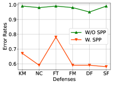
(a) CIFAR-100

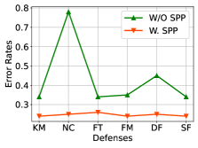
(b) HAM10000.

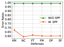
(c) Tiny ImageNet.

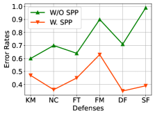
(d) Reuters.

Figure 5: SPP against Faker when $n=5$ and $m=1$. W. SPP means that the defenses are protected by SPP, and W/O SPP means that the defenses are not protected by SPP.

B.3 Extra Experiments on Faker

B.3.1 Datasets and Models

1) HAM10000 is a collection of 10,015 dermatoscopic images of common pigmented skin lesions with seven classes, containing 7000 training images and 3015 test images. This dataset is non-IID, which means that the amount of data in each category is obviously different. We use a 10-layer CNN neural network to categorize it. The details of the model are as follows. There are four Conv2D layers, two MaxPooling2D layers, one Flatten layer, and three Dense layers. 2) CIFAR-100 consists of 100 classes with 600 images per class, totaling 60,000 images. The dataset is designed to evaluate object recognition algorithms and covers a wide range of visual concepts, including animals, vehicles, household objects, and natural scenes. Each image is a 32x32 RGB image, making it a challenging dataset for machine learning models to classify objects accurately. An 8-layer CNN model is applied, including two Conv2D layers, two MaxPooling2D layers, one Flatten layer, and three Dense layers. 3) Tiny ImageNet is a downscaled version of the ImageNet dataset, which contains 200 classes, 100,000 training images, and 10,000 test images. All images in Tiny ImageNet are of 64x64 pixels. We apply ResNet-18 to process this dataset. 4) The Reuters dataset is a collection of short news articles that were published by Reuters in the 1980s. The dataset consists of 10,788 news articles, divided into a training set of 8,982 articles and a test set of 1,806 articles. We use an LSTM model to process this dataset.

B.3.2 Experimental Results

We follow the basic settings as in Section 6.1 to evaluate Faker and SPP with more experiments. Below are the experimental results.

Further Evaluation of Faker on MNIST, FMNIST, and CIFAR-10. We take Dirichlet distribution to obtain non-IID training data by setting the concentration parameter as 0.5, and we use LeNet-5 for MNIST, adjusted LeNet for FMNIST, and AlexNet for CIFAR-10. The experimental results are shown in Table 18, which indicates that Faker can undermine similarity-based defenses with different deep learning models and data distributions and Faker outperforms the benchmark attacks.

Table 18: Error rates of non-IID data obtained by Dirichlet distribution with $n=100$ and $m=20$, and the concentration parameter is $0.5$. The error rates of FA for the three datasets are 0.03, 0.18, and 0.43 when there is no attack.

Dataset	Attack	KM	NC	FT	FM	DF	SF
MNIST	N/A	0.07	0.03	0.03	0.03	0.03	0.03
	LA	0.07	0.03	0.03	0.03	0.03	0.03
	MB	0.07	0.03	0.03	0.03	0.03	0.03
	Faker	0.15	0.18	0.07	0.25	0.11	0.30
FMNIST	N/A	0.38	0.18	0.17	0.18	0.18	0.17
	LA	0.38	0.18	0.22	0.18	0.23	0.22
	MB	0.38	0.18	0.21	0.18	0.18	0.19
	Faker	0.57	0.64	0.51	0.63	0.76	0.90
CIFAR-10	N/A	0.86	0.43	0.44	0.43	0.42	0.77
	LA	0.90	0.43	0.80	0.49	0.73	0.90
	MB	0.90	0.43	0.68	0.47	0.64	0.90
	Faker	0.90	0.90	0.90	0.90	0.90	0.90

Table 19: Error rates of non-IID data based on CIFAR-100, HAM10000, Tiny ImageNet, and Reuters, with $n=5$ and $m=1$. The error rates of FA for the four datasets are 0.59, 0.25, 0.58, and 0.36 when there is no attack.

Dataset	Attack	KM	NC	FT	FM	DF	SF
CIFAR-100	N/A	0.67	0.59	0.78	0.59	0.59	0.58
	LA	0.99	0.59	0.85	0.90	0.59	0.99
	MB	0.99	0.58	0.82	0.87	0.59	0.99
	Faker	0.99	0.98	0.99	0.98	0.95	0.99
HAM10000	N/A	0.24	0.25	0.26	0.24	0.25	0.24
	LA	0.28	0.25	0.33	0.34	0.25	0.24
	MB	0.26	0.25	0.34	0.34	0.25	0.24
	Faker	0.34	0.78	0.34	0.35	0.45	0.34
Tiny ImageNet	N/A	0.68	0.58	0.61	0.60	0.60	0.60
	LA	0.93	0.72	0.84	0.73	0.69	0.99
	MB	0.82	0.65	0.79	0.71	0.63	0.99
	Faker	0.99	0.99	0.99	0.99	0.99	0.99
Reuters	N/A	0.47	0.36	0.45	0.63	0.35	0.39
	LA	0.57	0.36	0.64	0.64	0.38	0.99
	MB	0.51	0.36	0.64	0.63	0.37	0.99
	Faker	0.60	0.70	0.64	0.90	0.71	0.99

Evaluation of Faker on Other Datasets. Since the performance of all four datasets trained in the FL system decreases significantly in terms of accuracy as the number of users increases, we choose to set a smaller number of users to simulate the cross-silo FL case. We set $n=5$ and $m=1$, the other settings are the same as the experiments mentioned in Section 6.1. The results of the error rates are shown in Table 19. We can see that Faker outperforms the benchmark attacks on these datasets in decreasing test accuracy. The results in Table 16 show that Faker can always pass the detection of the defender. The results in Table 17 indicate that Faker is more time-efficient than the benchmark attacks.

Evaluation of SPP on Other Datasets. We also test SPP on these four datasets, and the results are presented in Fig. 5, which show that SPP is effective in mitigating the negative impacts of Faker on the global model.

Appendix C Future Research Directions

Below are several potential research directions.

In-depth Study of the Robustness of Similarity Metrics. In this paper, the robustness of the similarity metrics is analyzed only in the FL system, while more theoretical and experimental evaluations are required for its application when employed in other systems.

Adapting Faker to Undermine Other Similarity-based Mechanisms. Faker is not limited to launching adversarial attacks, but can also be used to assist clients in obtaining overrides during fairness assessments.

More Efficient Solutions for P0. In this paper, we take an approximate solution for P0, although experiments have shown that its performance meets the requirements for launching an attack, more efficient and accurate solutions may be required in the future.

Studying the Robustness of Other Evaluation Metrics. This paper is the first attempt to analyze the robustness of evaluation metrics in FL systems, while the robustness of other evaluation metrics is not yet clear.

References

- [1] Sana Awan, Bo Luo, and Fengjun Li. Contra: Defending against poisoning attacks in federated learning. In Computer Security–ESORICS 2021: 26th European Symposium on Research in Computer Security, Darmstadt, Germany, October 4–8, 2021, Proceedings, Part I 26, pages 455–475. Springer, 2021.
- [2] Eugene Bagdasaryan, Andreas Veit, Yiqing Hua, Deborah Estrin, and Vitaly Shmatikov. How to backdoor federated learning. In International Conference on Artificial Intelligence and Statistics, pages 2938–2948. PMLR, 2020.
- [3] Gilad Baruch, Moran Baruch, and Yoav Goldberg. A little is enough: Circumventing defenses for distributed learning. Advances in Neural Information Processing Systems, 32, 2019.
- [4] Peva Blanchard, El Mahdi El Mhamdi, Rachid Guerraoui, and Julien Stainer. Machine learning with adversaries: Byzantine tolerant gradient descent. Advances in Neural Information Processing Systems, 30, 2017.
- [5] Baturalp Buyukates, Chaoyang He, Shanshan Han, Zhiyong Fang, Yupeng Zhang, Jieyi Long, Ali Farahanchi, and Salman Avestimehr. Proof-of-contribution-based design for collaborative machine learning on blockchain. arXiv preprint arXiv:2302.14031, 2023.
- [6] Di Cao, Shan Chang, Zhijian Lin, Guohua Liu, and Donghong Sun. Understanding distributed poisoning attack in federated learning. In 2019 IEEE 25th International Conference on Parallel and Distributed Systems (ICPADS), pages 233–239. IEEE, 2019.
- [7] Xiaoyu Cao, Minghong Fang, Jia Liu, and Neil Zhenqiang Gong. Fltrust: Byzantine-robust federated learning via trust bootstrapping. arXiv preprint arXiv:2012.13995, 2020.
- [8] Xiao Chen, Haining Yu, Xiaohua Jia, and Xiangzhan Yu. Apfed: Anti-poisoning attacks in privacy-preserving heterogeneous federated learning. IEEE Transactions on Information Forensics and Security, 2023.
- [9] Siddharth Divi, Yi-Shan Lin, Habiba Farrukh, and Z Berkay Celik. New metrics to evaluate the performance and fairness of personalized federated learning. arXiv preprint arXiv:2107.13173, 2021.
- [10] empty. Reuters-21578 dataset, empty.
- [11] Minghong Fang, Xiaoyu Cao, Jinyuan Jia, and Neil Gong. Local model poisoning attacks to Byzantine-Robust federated learning. In 29th USENIX Security Symposium (USENIX Security 20), pages 1605–1622, 2020.
- [12] Minghong Fang, Jia Liu, Neil Zhenqiang Gong, and Elizabeth S Bentley. Aflguard: Byzantine-robust asynchronous federated learning. In Proceedings of the 38th Annual Computer Security Applications Conference, pages 632–646, 2022.
- [13] Yann Fraboni, Richard Vidal, Laetitia Kameni, and Marco Lorenzi. Clustered sampling: Low-variance and improved representativity for clients selection in federated learning. In International Conference on Machine Learning, pages 3407–3416. PMLR, 2021.
- [14] Clement Fung, Chris JM Yoon, and Ivan Beschastnikh. Mitigating sybils in federated learning poisoning. arXiv preprint arXiv:1808.04866, 2018.
- [15] Clement Fung, Chris JM Yoon, and Ivan Beschastnikh. The limitations of federated learning in sybil settings. In 23rd International Symposium on Research in Attacks, Intrusions and Defenses (RAID 2020), pages 301–316, 2020.
- [16] Rachid Guerraoui, Sébastien Rouault, et al. The hidden vulnerability of distributed learning in byzantium. In International Conference on Machine Learning, pages 3521–3530. PMLR, 2018.
- [17] Shanshan Han, Wenxuan Wu, Baturalp Buyukates, Weizhao Jin, Yuhang Yao, Qifan Zhang, Salman Avestimehr, and Chaoyang He. Kick bad guys out! zero-knowledge-proof-based anomaly detection in federated learning. arXiv preprint arXiv:2310.04055, 2023.
- [18] Guiqiang Hu, Hongwei Li, Tao Wu, Wenshu Fan, and Yushu Zhang. Efficient byzantine-robust and privacy-preserving federated learning on compressive domain. IEEE Internet of Things Journal, 2023.
- [19] Shengshan Hu, Jianrong Lu, Wei Wan, and Leo Yu Zhang. Challenges and approaches for mitigating byzantine attacks in federated learning. arXiv preprint arXiv:2112.14468, 2021.
- [20] Wenke Huang, Mang Ye, and Bo Du. Learn from others and be yourself in heterogeneous federated learning. In Proceedings of the IEEE/CVF Conference on Computer Vision and Pattern Recognition, pages 10143–10153, 2022.
- [21] Najeeb Moharram Jebreel and Josep Domingo-Ferrer. Fl-defender: Combating targeted attacks in federated learning. Knowledge-Based Systems, 260:110178, 2023.
- [22] Harsh Kasyap and Somanath Tripathy. Hidden vulnerabilities in cosine similarity based poisoning defense. In 2022 56th Annual Conference on Information Sciences and Systems (CISS), pages 263–268. IEEE, 2022.
- [23] Torsten Krauß and Alexandra Dmitrienko. Avoid adversarial adaption in federated learning by multi-metric investigations. arXiv preprint arXiv:2306.03600, 2023.
- [24] Alex Krizhevsky, Geoffrey Hinton, et al. Learning multiple layers of features from tiny images. 2009.
- [25] Alex Krizhevsky, Ilya Sutskever, and Geoffrey E Hinton. Imagenet classification with deep convolutional neural networks. Advances in neural information processing systems, 25, 2012.
- [26] Ya Le and Xuan Yang. Tiny imagenet visual recognition challenge. CS 231N, 7(7):3, 2015.
- [27] Yann LeCun, Léon Bottou, Yoshua Bengio, and Patrick Haffner. Gradient-based learning applied to document recognition. Proceedings of the IEEE, 86(11):2278–2324, 1998.
- [28] Yann LeCun and Corinna Cortes. MNIST handwritten digit database. 2010.
- [29] Qinbin Li, Yiqun Diao, Quan Chen, and Bingsheng He. Federated learning on non-iid data silos: An experimental study. In 2022 IEEE 38th International Conference on Data Engineering (ICDE), pages 965–978. IEEE, 2022.
- [30] Zhuoran Ma, Jianfeng Ma, Yinbin Miao, Yingjiu Li, and Robert H Deng. Shieldfl: Mitigating model poisoning attacks in privacy-preserving federated learning. IEEE Transactions on Information Forensics and Security, 17:1639–1654, 2022.
- [31] Ranwa Al Mallah, David Lopez, Godwin Badu Marfo, and Bilal Farooq. Untargeted poisoning attack detection in federated learning via behavior attestation. arXiv preprint arXiv:2101.10904, 2021.
- [32] Brendan McMahan, Eider Moore, Daniel Ramage, Seth Hampson, and Blaise Aguera y Arcas. Communication-efficient learning of deep networks from decentralized data. In Artificial intelligence and statistics, pages 1273–1282. PMLR, 2017.
- [33] Viraaji Mothukuri, Reza M Parizi, Seyedamin Pouriyeh, Yan Huang, Ali Dehghantanha, and Gautam Srivastava. A survey on security and privacy of federated learning. Future Generation Computer Systems, 115:619–640, 2021.
- [34] Thien Duc Nguyen, Phillip Rieger, Huili Chen, Hossein Yalame, Helen Möllering, Hossein Fereidooni, Samuel Marchal, Markus Miettinen, Azalia Mirhoseini, Shaza Zeitouni, et al. FLAME: Taming backdoors in federated learning. In 31st USENIX Security Symposium (USENIX Security 22), pages 1415–1432, 2022.
- [35] Xiaomin Ouyang, Zhiyuan Xie, Jiayu Zhou, Jianwei Huang, and Guoliang Xing. Clusterfl: a similarity-aware federated learning system for human activity recognition. In Proceedings of the 19th Annual International Conference on Mobile Systems, Applications, and Services, pages 54–66, 2021.
- [36] Ashwinee Panda, Saeed Mahloujifar, Arjun Nitin Bhagoji, Supriyo Chakraborty, and Prateek Mittal. Sparsefed: Mitigating model poisoning attacks in federated learning with sparsification. In International Conference on Artificial Intelligence and Statistics, pages 7587–7624. PMLR, 2022.
- [37] Saurav Prakash and Amir Salman Avestimehr. Mitigating byzantine attacks in federated learning. arXiv preprint arXiv:2010.07541, 2020.
- [38] Virat Shejwalkar and Amir Houmansadr. Manipulating the byzantine: Optimizing model poisoning attacks and defenses for federated learning. In NDSS, 2021.
- [39] Virat Shejwalkar, Amir Houmansadr, Peter Kairouz, and Daniel Ramage. Back to the drawing board: A critical evaluation of poisoning attacks on production federated learning. In 2022 IEEE Symposium on Security and Privacy (SP), pages 1354–1371. IEEE, 2022.
- [40] Ziteng Sun, Peter Kairouz, Ananda Theertha Suresh, and H Brendan McMahan. Can you really backdoor federated learning? arXiv preprint arXiv:1911.07963, 2019.
- [41] Philipp Tschandl, Cliff Rosendahl, and Harald Kittler. The ham10000 dataset, a large collection of multi-source dermatoscopic images of common pigmented skin lesions. Scientific data, 5(1):1–9, 2018.
- [42] Wei Wan, Shengshan Hu, Minghui Li, Jianrong Lu, Longling Zhang, Leo Yu Zhang, and Hai Jin. A four-pronged defense against byzantine attacks in federated learning. arXiv preprint arXiv:2308.03331, 2023.
- [43] Ning Wang, Yang Xiao, Yimin Chen, Yang Hu, Wenjing Lou, and Y Thomas Hou. Flare: Defending federated learning against model poisoning attacks via latent space representations. In Proceedings of the 2022 ACM on Asia Conference on Computer and Communications Security, pages 946–958, 2022.
- [44] Zhilin Wang, Qiao Kang, Xinyi Zhang, and Qin Hu. Defense strategies toward model poisoning attacks in federated learning: A survey. In 2022 IEEE Wireless Communications and Networking Conference (WCNC), pages 548–553. IEEE, 2022.
- [45] Han Xiao, Kashif Rasul, and Roland Vollgraf. Fashion-mnist: a novel image dataset for benchmarking machine learning algorithms. arXiv preprint arXiv:1708.07747, 2017.
- [46] Cong Xie, Sanmi Koyejo, and Indranil Gupta. Zeno++: Robust fully asynchronous sgd. In International Conference on Machine Learning, pages 10495–10503. PMLR, 2020.
- [47] Jian Xu, Shao-Lun Huang, Linqi Song, and Tian Lan. Byzantine-robust federated learning through collaborative malicious gradient filtering. In 2022 IEEE 42nd International Conference on Distributed Computing Systems (ICDCS), pages 1223–1235. IEEE, 2022.
- [48] Dong Yin, Yudong Chen, Ramchandran Kannan, and Peter Bartlett. Byzantine-robust distributed learning: Towards optimal statistical rates. In International Conference on Machine Learning, pages 5650–5659. PMLR, 2018.
- [49] Hao Yu, Chuan Ma, Meng Liu, Xinwang Liu, Zhe Liu, and Ming Ding. G2 uardfl: Safeguarding federated learning against backdoor attacks through attributed client graph clustering. arXiv preprint arXiv:2306.04984, 2023.
- [50] Jiale Zhang, Junjun Chen, Di Wu, Bing Chen, and Shui Yu. Poisoning attack in federated learning using generative adversarial nets. In 2019 18th IEEE International Conference On Trust, Security And Privacy In Computing And Communications/13th IEEE International Conference On Big Data Science And Engineering (TrustCom/BigDataSE), pages 374–380. IEEE, 2019.
- [51] Yue Zhao, Meng Li, Liangzhen Lai, Naveen Suda, Damon Civin, and Vikas Chandra. Federated learning with non-iid data. arXiv preprint arXiv:1806.00582, 2018.
- [52] Xingchen Zhou, Ming Xu, Yiming Wu, and Ning Zheng. Deep model poisoning attack on federated learning. Future Internet, 13(3):73, 2021.