Impact of a mean field dynamo on neutron star mergers leading to magnetar remnants
Abstract
We investigate the impact of a mean field model for the -dynamo potentially active in the post-merger phase of a binary neutron star coalescence. We do so by deriving equations for ideal general relativistic magnetohydrodynamics (GRMHD) with an additional term, which closely resemble their Newtonian counterpart, but remain compatible with standard numerical relativity simulations. We propose a heuristic dynamo closure relation for the magnetorotational instability-driven turbulent dynamo in the outer layers of a differentially rotating magnetar remnant and its accretion disk. As a first demonstration, we apply this framework to the early stages of post-merger evolution (). We demonstrate that depending on the efficacy of the dynamo action, magnetically driven outflows can be present with their amount of baryon loading correlating with the magnetic field amplification. These outflows can also contain precursor flaring episodes before settling into a quasi-steady state. For the dynamo parameters explored in this work, we observe electromagnetic energy fluxes of up to , although larger amplification parameters will likely lead to stronger fluxes. Our results are consistent with the expectation that substantial dynamo amplification (either during or after the merger) may be necessary for neutron-star remnants to power short gamma-ray bursts or precursors thereof.
I Introduction
Neutron stars not only feature some of the most extreme conditions for nuclear matter but can also contain some of the strongest magnetic fields in the universe [1]. In the context of neutron star mergers, magnetic fields are crucial for driving electromagnetic counterparts such as kilonova afterglows [2] and gamma-ray bursts [3], see also GRB170817A for a short-duration gamma-ray burst jointly detected with a gravitational wave event [4].
Based on long-term simulations of neutron star – black hole coalescence [5, 6, 7], it has recently been suggested that while long gamma-ray bursts may be powered by black hole disk systems, short gamma-ray bursts may require the presence of a magnetar engine [8]. However, the precise conditions and timescales probed in the simulations underlying these conclusions may sensitively depend on the magnetic field geometry produced in the collisions [9, 10, 11, 12, 7], with additional uncertainties coming from pre-merger fields [13, 11] (see also Refs. [14, 15, 16, 17]).
Furthermore, the presence of a blue component in the electromagnetic afterglow of GRB170817A appears to require additional magnetic and neutrino-driven mass ejection, likely to originate from the surface of a hot hypermassive neutron star (HMNS) formed in the merger [18, 19, 20, 21, 22]. Recent numerical relativity simulations of this process seem to support this conclusion [23, 24, 25].
However, our understanding of the dynamics and evolution of the magnetic field in such a magnetar merger remnant remains incomplete. This is largely a result of underresolved dynamo physics during the merger [26, 27] and inside the post-merger remnant [28, 29]. Although small-scale dynamo processes at merger seem to be driven by Kelvin-Helmholtz instabilities at the shearing interface layer between the two stars [27], the effect of macroscopic amplification in the bulk of the star remains uncertain [30]. Similarly, additional processes such as Rayleigh-Taylor instabilities on stellar surfaces may contribute to the overall amplification [31]. Recently, very high-resolution numerical relativity simulations of the post-merger remnant have been reported to show the presence of a magnetorotational instability [32] (MRI)-driven dynamo [33], which may also depend on the chemical stratification present in the remnant [34], see also [35]. Similar processes may also operate in the accretion disk [36, 37, 38]. Clarifying the precise impact of such under-resolved processes on the neutron star remnant will be central to our understanding of whether magnetar engines formed in mergers can power short gamma-ray bursts. This is particularly relevant, as the neutrino-driven stellar winds may strongly baryon load the outflows, potentially lowering the luminosity [39, 19, 21].
Incorporating under-resolved dynamo physics into neutron star mergers is challenging. Previous effective numerical models have resorted to simple exponential modifications of the evolution equations [40, 41], or have made use of effective Large-Eddy approaches [42, 43]. Others, inspired by studies of accretion disk dynamos [44, 45, 46], have used effective mean field models [47]. Here, we follow the latter approach but focus mainly on the ability of launching winds and jet-like outflows from the surface of the hypermassive neutron star. Due to the natural shearing background present in the differentially rotating remnant star [48, 49], one possibly active mechanism for mean field amplification is the dynamo [50, 51]. Recent works have shown that the presence of such an effect inside the outer layers of the neutron star can lead to magnetic field breakout and the launching of (intermittent) jet-like outflows [52, 33].
Effective models including mean field -terms in numerical simulations have been developed by
various communities for applications ranging from early universe cosmology
[53], galaxy dynamics [54], to supernovae
[55] and compact objects [44, 46, 47].
While most of these formulations have considered Newtonian magnetohydrodynamics (MHD), in which the inclusion of an effective
electromotive force can be straightforward, the relativistic
context poses extra challenges.
Previous approaches have chosen to
include effective - and Hall terms in a dynamical Ohm’s law [44, 47].
In the relativistic context, this requires the solution of an
additional evolution equation for the electric field, which becomes
numerically stiff in the perfectly conducting limit, and requires implicit
time stepping to be handled stably [56, 57].
On the other hand, these approaches have been demonstrated to have no well-posed initial value
problem [58]. Although from a physics point of view full dissipative approaches might be more desirable [59, 60], the
additional computational overhead and the loss of robustness established for GRMHD simulation [61], makes this less appealing, especially when full nonideal effects are not required for the numerical modeling.
Complementing these works, we here present a new formulation to systematically incorporate the effect into numerical general relativistic MHD simulations. Together with the shear flow naturally present in the post-merger system, this naturally enables a subgrid model for the -dynamo. While the formulation is generic, we apply it here specifically to the case of a post-merger magnetar remnant.
Our paper is structured as follows. In Sec. II we present the general approach to modeling the effect, before introducing a generalization to the relativistic regime. We then discuss a heuristic subgrid model, before outlining the particular steps needed to incorporate them into a numerical relativity code. In Sec. III, we present an initial assessment of this model in the early post-merger phase of a magnetar remnant.
II Methods
In this work, we study the impact of a mean field dynamo model on the evolution of a magnetar remnant formed in a neutron star collision. To this end, we have implemented a new approach to incorporating subgrid dynamo models, in particular, the effect into non-resistive general-relativistic magnetohydrodynamics (GRMHD) simulations. In the following, we will first describe a formulation of the effect in Sec. II.1, before providing details on the numerical implementation and simulation setup in Sec. II.4.
As the main theoretical framework for modeling the evolution of stellar matter, we solve the Einstein-Maxwell-Fluid system in a magnetohydrodynamic approximation [62]. More specifically, we solve
| (1) | |||
| (2) | |||
| (3) |
where is the Einstein tensor, , and , are the Maxwell tensor and its dual. Introducing the fluid four-velocity , we can decompose the field strength tensor into comoving electric, , and magnetic, , fields [63],
| (4) | ||||
| (5) |
Here is the four-dimensional Levi-Civita tensor. We further assume that the plasma dynamics are governed by a perfect fluid described by its rest-mass density, , total energy density , and pressure , in addition to its fluid four-velocity, . The combined system is described by the total energy-momentum tensor
| (6) |
In order to evolve the system (1)-(3), we need to specify closures for the pressure and electric field. For a non-resistive plasma, we need not evolve the electric field independently. In other words, we need to provide an equation of state, , and a relation 111We point out that alternatively, in a resistive approach, we could also solve an evolution equation for the electric field , which would couple to the fluid via an Ohm’s law [56, 44, 64, 65, 57] However, here we consider the perfectly conducting ideal-MHD limit appropriate for neutron star mergers [66]..
II.1 Subgrid dynamo physics
We now want to provide a brief summary of mean field dynamo theory. For further background, see, e.g., Ref. [67] for a review. To better illustrate the approach taken here, we first review a Newtonian formulation of the problem, before doing the same in a fully covariant, general-relativistic context.
Consider the flat space evolution equation for the magnetic field ,
| (7) |
where is the Levi-Civita tensor. Consistent with the high conductivity found inside neutron stars, we further assume the ideal MHD limit , where is the 3-fluid velocity [68]. The main reasoning behind dynamo mean field theory is to capture the effect of (small-scale) fluctuations operating on top of a background mean field. To this end, one may decompose the magnetic and velocity fields
| (8) | ||||
| (9) |
into an averaged mean field , and small fluctuations , such that on average and , respectively. When evaluating the effective mean electric field, in the same way, one finds that
| (10) |
Although individual fluctuations vanish, their second-order correlation does not. In mean field dynamo theory, this system is now closed by performing a first-order expansion of these fluctuations in terms of the mean magnetic field [69],
| (11) | ||||
| (12) |
where we have introduced tensorial mean field dynamo coefficients and . Indeed, for certain processes such as magnetorotational instability-driven dynamos, can be computed from local simulations [70]. In the last line, we have used that in the small velocity limit , where is the electric current. In summary,
| (13) |
From Eq. (13) it is now apparent that acts as
an effective anisotropic resistivity.
We now want to generalize the forgoing discussion to the relativistic context. In doing so, we effectively have two options. We could consider fully covariant first-order perturbation theory [71], or instead choose to generalize the Newtonian expressions (12) and (13), which we pursue. While our approach is similar to the one put forward by Ref. [44] (see also Ref. [47]), we will make further simplifications concerning the resistive timescales of the plasma. These will allow us to obtain equations that do not suffer from stiffness problems in the ideal MHD limit and do not require implicit time stepping [72]. Our discussion begins with a dynamical Ohm’s law inspired by relativistic 14-moment closure theory [60], which we have supplemented with tensorial mean field dynamo terms and ,
| (14) |
where is the electric current, the electric resistivity, is the mean electric field and . We have also introduced a collisionality timescale . These quantities are by definition projected into the fluid frame by means of the mean four-velocity of the fluid . This implies that . In the following, we shall drop any explicit notation of mean field quantities for improved readability. We now make several assumptions, applicable to the case of neutron star merger dynamics. Firstly, we assume that the collision timescale, , associated with the mean-free path of the system, is much shorter than large-scale variations of the system [66]. In this limit, we may neglect the term on the left-hand side in Eq. (14). We caution, however, that without further simplifications concerning the resistivity, , the system would likely lose strong hyperbolicity [58], though in practice numerical solutions of this system can still be found [56, 44, 65, 57]. Alleviating this fact, and in line with the almost perfect conductivity encountered in neutron star matter [66], we will now reduce the equations to their non-resistive limit, . To this end, we re-write
| (15) |
where . We can now see that the -effect creates an anisotropic conductivity (similar to the Hall effect [68]). Indeed, such effects have been studied in the context of shear-current dynamo amplification [73]. In this work, we do not consider such effects and will only study the limit where the mean field dynamo operates on timescales much longer than the effective resistive timescale. In proceeding along these lines, we now make the crucial assumption that dynamo effects will always grow relative to the resistive timescale. In other words, does not vanish in the limit of zero resistivity. This is a well-justified assumption if we consider modeling an ultimately kinematic dynamo, which will operate on viscous scales larger than the resistive scale [35]. This allows us to re-express the comoving electric field as,
| (16) |
where we have re-expressed . Eq. (16) is the constitutive closure relation of our mean field dynamo model. This lets us draw an important conclusion, for the approximations we make. Since we assume that we are essentially always nonresistive, any nonideal dynamo growth of the magnetic field must come from a nonzero -term, i.e. nonvanishing components of . As we will see later on, making this assumption allows us to use an ideal GRMHD code, with only minor modifications.
II.2 3+1 mean field dynamo equations
Having outlined the form of the above equations, we next proceed to recast them into a form suitable for numerical integration. This is done in two steps. First, we will show that the dynamo action (16) does not require us to evolve the electric field itself, but rather will lead to ideal-MHD-like closure relations. In the second step, we highlight modifications to the GRMHD equations necessary to include these effects. In the following, we adopt the ADM split of spacetime [74], where is the lapse function, the shift vector, and the spatial metric.
While our dynamo closure (16) links comoving electric and magnetic fields, we need to recover the electric, , and magnetic, , fields as seen by a Eulerian observer corresponding to the space-time normal . Using these definitions, we can compute
| (17) |
where we have used that , as well as the dynamo relation (16). We have also introduced the three-dimensional Levi-Civita tensor embedded in a four-dimensional space, , as well as the Lorentz factor, . It is also convenient to introduce the spatial velocity . Next, we need to solve this equation for , so that we can express the comoving magnetic field in terms of ,
| (18) | ||||
| (19) |
where is the comoving magnetic field in ideal (non-resistive) GRMHD [62], and is the fluid-frame projector. We point out that as a geometric series, Eq.(19) will converge as long as the dynamo timescales are much longer than the resistive timescale, i.e., . Furthermore, the expansion in fundamentally preserves covariance of the equations, but will make the solution inaccurate should the dynamo begin to act on timescales comparable to the resistive scale.
II.2.1 A pseudo-scalar dynamo model
While modeling specific dynamo processes, such as those associated with the MRI, will require anisotropic dynamo coefficients [70, 75], incorporating anisotropic dynamo terms will require more substantial modifications to existing GRMHD codes, similar to using a fully resistive [56, 44, 57, 47], or a dissipative MHD code [76]. Circumventing these challenges, in this first application of this model we will restrict ourselves to a simplified dynamo model commonly employed in cosmology [53], supernova [55], and relativistic contexts [46]. For a (pseudo-)scalar effect, , the equations simplify considerably. In the following, we, therefore, assume
| (20) |
Using this definition, we can easily see that
| (21) |
which leads to an electric field in the normal observer frame,
| (22) |
which we have expanded to leading order in . This expression is remarkably similar to the Newtonian limit given in Eq. (13) (in the absence of a -term), which it recovers in the small velocity limit,
| (23) |
We point out that despite the apparent expansion in both expressions (23) and (22) are fully covariant, but correspond to either the full or only partial first-order contribution in in Eq. (19). For the background flows inside the hypermassive neutron star remnants , we likely do not expect a large difference between the two approximations. For completeness, we opt to use Eq. (22) and
| (24) |
Similarly, the stress-energy tensor results in
| (25) |
which is consistent with ideal GRMHD. In the scalar limit, the comoving electric and magnetic fields always line up, so that no effective heat flux contributions are present. This is equivalent to stating that the presence of the scalar dynamo terms does not induce a nonideal Poynting flux , which gets modified in the anisotropic case.
It is instructive to compare this formalism with previous approaches to modeling scalar -dynamo effects in the GRMHD literature [44, 46, 47]. Essentially, the starting point for these formulations is a fully resistive description, where the dynamo term is included as part of the Ohms law (14). The advantage of such an approach is that the resistive timescale can be explicitly fixed, allowing dynamo amplification (to all orders in ) to occur on fully controllable timescale, whereas in our approach only fixes the ratio of the dynamo growth time to (effectively) numerical resistivity. On the other hand, our approach allows us to only minimally modify the ideal GRMHD equations, while the resistive equations become stiff in the perfectly conducting limit and require special numerical treatment [56].
II.3 Subgrid model parameters
Having described the method, the final step in completing this model is a specification of the dynamo closure parameters. These will strongly depend on the microphysics that is being modeled. In the case of relativistic accretion disks, the capture of under-resolved MRI turbulence has been accomplished using different prescriptions [45, 46], which have been tested against full three-dimensional resolved simulations, or have been inspired by local shearing box calculations [70, 77]. Rather than relying on such calculations, which may not directly translate to the HMNS case, we take values inspired by a recent very high-resolution simulation [33]. There it was found that the outer (MRI unstable) layers of the neutron-star remnant can drive a large-scale dynamo [33]. These results further imply that
| (26) |
where we point out that is a pseudo-scalar and has dimensions of a velocity, which we express relative to the speed of light. We caution that in our case is defined with the opposite sign and also includes an effective resistivity contribution that we have absorbed into the above expression. While determines the growth rate of the dynamo, it does not restrict its saturation level. Physically, saturation is expected to happen when the relevant reservoir of (largely kinetic) energy is converted into magnetic energy. In the absence of this self-limiting feedback on the mean field dynamo term when is prescribed, saturation has to be imposed manually using different criteria. In practice, we opt to limit
| (27) |
where is an indicator function for saturation, which is reached for . The formalism presented here will work for every choice of . For our specific application, we now suggest a phenomenological model for the saturation function inspired by very high-resolution simulations [28]. When using several prescriptions of , we opt to use Eq. (27) jointly over all them.
-
1.
Magnetization-dependent saturation limit
Here we limit based on the strength of the generated radial magnetic field . This is meaningful since the dynamo should generate a radial magnetic field only up to a fraction of the toroidal field, . If then the -effect would continue to generate more toroidal field via an dynamo, which is not supported by global simulations [33]. We in turn adopt,
(28) where is the fraction of radial magnetic field.
-
2.
Turbulent energy limit
In principle, the dynamo should be fueled by the available turbulent energy in the flow. Defining this number is not trivial and has been extensively investigated in the Newtonian large-eddy literature [78, 79, 80, 81]. The major challenge lies in defining what fraction of the turbulent kinetic energy is available to be converted into magnetic energy, as well as estimating the available turbulent kinetic energy in the first place
Assuming that the driving and decay (to smaller scales) of kinetic energy are in steady state, we can show that the saturation-level magnetization should be determined by the turbulent kinetic energy. More specifically, we find that (see Appendix A),
| (29) |
where is an effective mixing length, the fraction of turbulent kinetic energy converted into magnetic energy, and is the shear stress tensor. The dynamo should then saturate, when the turbulent energy budget has been used up, i.e., when
| (30) |
where is the magnetization. Local fluctuations in these quantities sometimes lead to large spurious values in individual grid cells. As a safety measure, we decided to cap the reference magnetization accordingly, i.e., enforce .
Effective saturation closure
In practice, subgrid models may be useful in capturing the effective mixing length of MRI-driven turbulence. From a first-principles point of view, the turbulent mixing length should be limited by the largest wavelength, , of the poloidal MRI [82],
| (31) |
where is the Alfven speed in the poloidal direction. However, this is not a robust criterion in low-resolution simulations, since . In other words, if is not fully developed in a low resolution simulations, the mean field feedback (that may contribute to its development) would not set in, self-limiting the applicability of the mean field prescription. We therefore opt to not use a magnetic field-dependent sub-grid model. Based on very high-resolution simulations of a neutron-star merger remnant [28], Ref. [83] has proposed a density-dependent fit formula for , which is given by
| (32) | ||||
where , and [83]. This prescription matches in a certain density regime but is independent of the local magnetic field in the simulation (see Fig. 1). Therefore, we opt to use as the fiducial sub-grid model in this work.
Saturation limit: Finally, we need to quantify the uncertainty factor within the model. This is necessary for a number of reasons. First, for algorithmic simplicity, we have assumed a steady state for the turbulent kinetic energy, which is likely not true and will depend on the effective scales probed by the models (in our case the numerical grid scale). Indeed, when considering large eddy simulations of post-merger magneto-turbulence, the kinetic energy and especially the amount of turbulence seems to depend on the numerical resolution [42, 30]. Secondly, the assumption of the turbulent mixing length model, , is a simplification based on the extraction of a viscous -parameter from a single high resolution simulation. While those effective scales should be correlated, they do not necessarily need to coincide, and may be different depending on the system parameters (equation of state, field topology, …). Since these uncertainties both enter quadratically in the saturation value of the magnetization, they may lead to significant under- or overestimations of the saturated state. In the absence of a systematic high-resolution comparison of such effective models, we opt to carry out a very rough estimate of by comparing our prediction for the saturated field strength, , due to turbulent amplification, with those observed in very high resolutions simulations [27, 28, 33]. To aid this comparison, we also compute the overall equipartition field strength , which may serve as an absolute upper bound. The resulting outcome is shown in Fig. 2. We can see that in the outer MRI-unstable layers, where the dynamo is presumably active [33], the equipartition field strength reaches .
Such high fields seem indeed to be produced in Ref. [33] (though not at lower resolution simulations using large-eddy closures [30]). This is also consistent with the launch of a relativistic outflow, which requires the remnant to enter a magnetically dominated regime in the outer layers [52, 25, 33]. Evaluating our estimate of dynamo saturation, we can further see that for the background probed in the post-merger remnant, . This implies that the dynamo model itself likely underproduces the necessary magnetic field strengths, and can only jump start the self-consistent evolution to higher field strengths via magnetic winding [84]. This leads us to assume, that we likely underestimate the amount of turbulent kinetic energy from the low resolution simulations. At the same time, the use of implies an implicit assumption on the resolution used to compute it. In other words, if the resolution was gradually increased the dynamo model needs to gradually switch off, meaning that has to decrease with increasing resolution. Consequently, we heuristically introduce a dependence on the numerical grid resolution, , by assuming that
| (33) |
where the resolution reference scale is set by the resolution used in Ref. [28] from which the fit was obtained. Overall, this leaves us with a prescription
| (34) |
We caution that this estimate does not rely on first-principles assumptions but mainly on conclusions drawn from the few available high-resolution simulations in the literature. Consequently, in this work we focus on understanding the qualitative impact of such a dynamo prescription, rather than quantitative aspects. In particular, our simulations will focus on understanding the role of and the saturated state of the dynamo.
Projected impact of the model Finally, we estimate the impact of this model. We do so by providing a back-of-the-envelope estimate for the flows present in the HMNS. In general, we can estimate the characteristic magnetization limit as , where is the average velocity of the turbulent flow, the characteristic gradient scale, and the average turbulent mixing scale. Assuming that characteristically inside the merger remnant, we find
| (35) |
This simplified model for constant mixing length is what we had previously explored in Ref. [52], demonstrating that this will lead to postmerger flaring and the launch of a steady-state relativistic outflow.
II.4 Numerical implementation
We now want to provide a brief description of how to implement the dynamo-augmented GRMHD equations into a numerical code. We will focus mainly on differences from standard GRMHD approaches and refer to the literature for further details on numerical implementations of ideal GRMHD (e.g., Ref. [62]).
In our implementation, we solve the Maxwell equations by evolving a covariant vector potential , such that , and is the scalar potential [85]. Adopting Lorenz gauge, , the evolution equations for the Maxwell sector are then given by [86],
| (36) |
We solve the discrete form of Eq. (36) on a staggered mesh [85], where the electric and magnetic fields are treated using high-resolution shock capture methods [87]. More precisely, we adopt the upwind constraint transport method of Ref. [88], as implemented in the ECHO scheme [89]. An extension to non-ideal electric fields is straightforward [90]. No other modifications of the Maxwell equations are necessary to incorporate the scalar dynamo term, besides Eq. (24). On the hydrodynamics side, the rescaling of the magnetic field needs to be carried out following Eqs. (II.2.1) and (22).
One important aspect of the GRMHD equations in flux-divergence form is the need to recover primitive variables from a conserved state [91]. To use standard algorithms for primitive recovery [92], it is necessary to decouple the direct dependence of the dynamo coefficient onto the fluid state. To this end, , cannot directly depend on the primitive variables . Rather than specifying a closure relation for , we artificially introduce a rate equation, enforcing that relaxes to the desired closure relation over a timescale ,
| (37) |
which corresponds to a simple advection equation with a relaxation term. The relaxation time is a free parameter, which for simplicity we will choose to be a constant.
We stress that due to the approximate nature of the dynamo closure relation the small time lag in relaxing to the desired value will likely have only a negligible effect on the simulation. At the same time, the ability to use extremely robust primitive recovery routines only available for the ideal GRMHD system (see Ref. [57] for challenges in resistive GRMHD versions) is crucial to successfully performing simulations of strongly magnetized flows when nuclear equations of state are used [61].
II.5 Simulation setup
We solve the discrete form of the magnetohydrodynamics sector using the Frankfurt/IllinoisGRMHD (FIL) code [93, 94]. FIL utilizes the ECHO scheme [89], implemented with a fourth-order accurate flux correction, fifth-order WENO-Z reconstruction [95], and HLLE Riemann solver [96]. Unlike previous GRMHD simulations with the code [93, 12, 97], we have upgraded the conservative-to-primitive inversion following the method of Kastaun et al. [92]. This method increases the overall accuracy of the code in highly magnetized regions (see also [61]), and has allowed us to study flaring and jet launching from neutron star merger remnants [52]. FIL also implements its own fourth-order accurate dynamical spacetime solver using the Z4c formulation [98, 99]. FIL operates on top of the EinsteinToolkit framework [100] and utilizes its moving-box mesh-refinement infrastructure Carpet [101].
The initial data for the simulation is computed using the FUKA code [102], which works on top of the Kadath framework [103]. Differently from our previous work [52], we consider a system with a long-lived remnant. We adopt the DD2 equation of state [104] with a total binary mass of , leading to a stable remnant neutron star. In terms of the initial mass ratio, we adopt . We initialize the magnetic field inside the two stars using a dipole magnetic field, prescribing the axisymmetric component of the vector potential in each star, [9], where is the cylindrical radius, and is the maximum pressure inside each star. We choose separately for each star, such that the maximum value of the magnetic field inside each star is .
We set up the numerical grid as a set of seven nested grids, which extend to an outer separation of about . The finest resolution has been chosen to be , which increases by a factor of two on every succinct level. In a previous work, we have demonstrated the use of fully high-order methods leads to a better capturing of the MRI in the disk at lower resolutions [93]. On the other hand, properties such as the time of jet launching and the amount of self-consistent amplification may not be well captured compared to high-resolution simulations [30]. However, the resolution considered here will be sufficient for a first assessment of difference subgrid prescriptions for the -dynamo.
III Results
Here we present the results of our numerical tests of different subgrid models for the -dynamo. We focus on the case of a long-lived magnetar remnant, where strong dynamo amplification could be present [33], aiding the launching of magnetically driven winds and jet-like outflows from the remnant [23, 52, 25].
We summarize our discussion and motivation detailed in Sec. II as follows: One of the main goals of this paper is an initial investigation of the - mean field dynamo model proposed in Sec. II. Although the growth rate we use is loosely based on recent conditions inferred from high-resolution simulations [28, 33], saturation of the dynamo cannot be self-consistently achieved in our model and needs to be prescribed. One of the main features of the dynamo subgrid model is that saturation is achieved once the available reservoir of turbulent kinetic energy has been converted into magnetic energy. In the case of the MRI this will happen only in regions of radially outward decaying differential rotation, which only cover the outermost layers of the star [48]. Within these regions, in principle, the total available kinetic energy associated with the differential rotation can be converted. Within the turbulence-inspired subgrid model we use, the saturation uncertainty is prescribed by rescaling the target magnetization using the parameter . Barring the availability of a large set of high-resolution simulations necessary for a thorough calibration of this parameter, here we investigate three different choices, corresponding to different regimes produced in our standard-resolution simulations. In this case our simulations should be regarded as complementary but not equal to recent high resolution works in the literature [42, 29, 43, 33].
We begin by discussing various properties of the evolution of the system associated with the dynamo subgrid model. Our discussion generally begins in the early post-merger phase, when we activate the dynamo model. A general description of the pre-merger and post-merger evolution of such systems can be found elsewhere (see, e.g., Refs. [1, 105] for recent reviews).
III.1 Saturation of the -dynamo
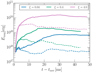
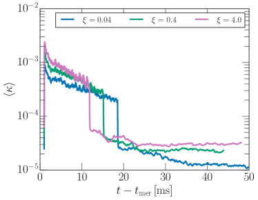
Shortly after the merger, we turn on the sub-grid dynamo model. The dynamo will be active in the outer layers of the star and disk with the precise density dependence largely governed by Eq. (34). In the differentially rotating background flow, the term will introduce an effective -dynamo. This will lead to an initial rapid growth, particularly of the poloidal magnetic field component, since the background field is largely toroidal [106, 30]. Fig. 3 shows the evolution of the magnetic energy for all three cases considered here. Depending on the parameter, , corresponding to the fraction of converted kinetic energy, the poloidal energy (dashed lines) is indeed undergoing an initial amplification phase. Afterward, the poloidal energy saturates rapidly, but the toroidal field continues to grow. The growth is driven in the following way: In the sheared background flow, the poloidal field is wound-up leading to linear magnetic field growth due to magnetic braking [84]. At the same time, the mean field dynamo needs to sustain the poloidal field. We can more quantitatively establish this by comparing the magnetic field evolution with the duty cycle of dynamo term, as expressed in a density-weighted average (Fig. 4). In fact, the main dynamo amplification is turned off early, and all models reach a saturated dynamo state between after the dynamo was activated. Indeed, this is consistent with fixing the growth rate of the dynamo via a globally constant parameter, which only switches off at saturation. We can see that coincident with the saturation of the mean field dynamo, the magnetic-field amplification slows down and at most follows a relation consistent with magnetic braking, or it stops entirely. The saturation levels of the magnetic energy are of the order of the fraction of converted kinetic energy, although the fractions with seem to approach a similar saturated state at late times, as a result of subsequent self-consistent magnetic field evolution.
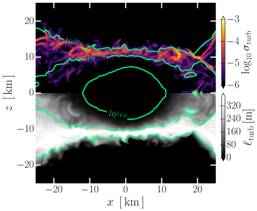
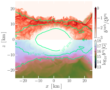
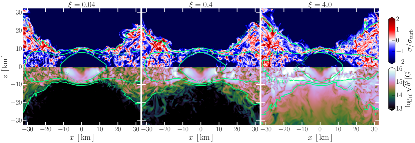
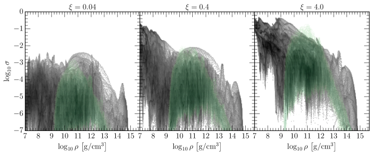
We can more quantitatively understand the saturation properties by considering the spatial distribution of the saturated magnetization inside the neutron-star remnant (Fig. 5). We can see that in the saturated state large regions close to the surface of the star and disk have undergone dynamo amplification. Further self-consistent magnetic field evolution has then taken over and has managed to amplify the field beyond the prescribed saturation level, typically by about an order of magnitude. We find that the local field strength close to the surface of the star can reach for weak amplification, and exceed for strong amplification. Within our discussion about expected saturated field strength (Fig. 2), these levels are higher than what the prescribed mean field dynamo can achieve on its own, given the imposed saturation bound. This is fully consistent with subsequent amplification being active by means of winding. The major difference between the simulation with varying subgrid parameter is the presence of substantial amplification in the disk region, at distances from the origin. Here, in the case of weak dynamo driving, no substantial amplification is active. In the other cases, additional amplification is present, enhancing the magnetic field strength in the disk. Since winding would be active in either case, it seems likely that additional amplification has aided the growth (and numerical capture) of the MRI in these regions (see also [107, 93]). In the strongest magnetic field case, this leads to a clear breakout of the field not only from the stellar surface but also from the disk region, injecting substantial fields of there. We can quantify this more explicitly by comparing the injection of field with the dynamo subgrid model to the actual magnetizations reached in the remnant. In Fig. 6 we do so, showing the distribution of the magnetization of fluid cells from the remnant as a function of density. We can clearly see the dynamo injection range acting on densities between . In the intermediate and strong amplification case, we can see that magnetization cascades to lower densities, driving amplifications in layers with densities . To sustain amplification in those regions, significant mixing of matter in denser layers with low density layers needs to happen. This may be associated with spiral winds injecting magnetized material into the disk [108, 109]. This leads us to speculate that dynamo amplification in intermediate layers of the star may qualitatively affect the outcome of a neutron star merger simulation.
III.2 Breakout of the magnetic field and flaring emission
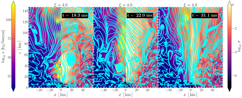
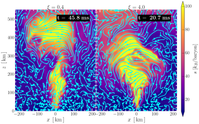
Two of our models feature break-out of the magnetic field and the launching of a mildly relativistic magnetically driven outflow. In the following, we will provide a brief description of this launching mechanism, and also describe the emission of flares which could power precursors to short gamma-ray bursts [52]. We begin by illustrating the breakout mechanism using the highest dynamo amplification case, . After an initial amplification of the magnetic field due to the mean field dynamo, the toroidal field gets significantly amplified due to magnetic braking [84]. At some point, the magnetic pressure in the toroidal field is substantial to make field lines rise magneto-bouyantly by means of a Parker instability [110]. See also Ref. [111] and [52] for simulations of the Parker instability in isolated and remnant neutron stars. In Fig. 7, we show that for our present simulations the initially confined magnetic field will magneto-bouyantly rise, emerging as closed loops connected to different points at the surface of the star. This can most easily be seen in terms of the entropy tracing out these magnetically dominated flux tubes (left panel). Differential rotation of the star will further inflate these loops. After a relative twist of about , the base field lines of the flare will reconnect, leading to the ejection of post-merger flares [52]. This observed mechanism is overall very similar to the reported phenomenology in simulations of magnetar giant flares [112, 113, 114], and precursor flares from in the inspiral of a neutron star binary [115, 116, 17]. While this process could in principle also driven by chemical gradients, these parts of the remnant are stable against convection consistent with recent finidings of stable stratification inside the remnant [34]. In our present simulations, we observe about three flaring events. We show the large-scale morphology of these flares in Fig. 8. We find that the emission of flares in both cases is intermittent, and their strength depends on the dynamo action. We will discuss this in more detail in Sec. III.3.
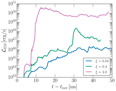
After launching of initial flares, these are immediately followed by an intermittent magnetically dominated outflow, leading to an initial collimation of the polar magnetic field (middle panel, Fig. 7). This collimation resembles a magnetic tower configuration [117] (see also Refs. [118, 119] for a discussion in the neutron star context). Eventually, this outflow relaxes to a steady state (see Fig. 12), whose properties we discuss further in Sec. III.3. While initially the polar outflows are magnetically dominated, the increase in mass ejection rate leads to a reduction of the magnetization making the outflow at late times less magnetized. This effect of baryon loading polar outflows is consistent with previous simulations of proto-neutron stars [39], and will eventually lead to a decline in the electromagnetic Poynting flux observed in this system (Fig. 11), see also Ref. [21]. We stress that this effect could be further enhanced if neutrino absorption was included in our simulations [24].
III.3 Magnetically driven winds and outflows
Shortly after the initial break-out of the magnetic field from the magnetar remnant, a quasi-steady magnetically driven polar outflow begins to develop. Such an outflow may be crucial in order to explain a neutron-poor component of the kilonova afterglow [21, 23, 25, 24]. In addition, the outflow may carry substantial electromagnetic (Poynting) flux, making it potentially relevant in the context of short gamma-ray burst production [25, 52, 33]. In the following, we want to provide a brief description of the polar outflow properties and their dependence on the dynamo parameter.
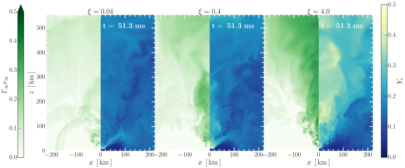
We begin by discussing the overall baryon loading and energetic properties of the outflow, such as the terminal Lorentz factor, (Fig. 9). We can estimate the terminal velocity using the conservation of Bernoulli’s constant , where is the specific enthalpy, which serves as an upper bound on if fully converted into a kinetic energy at large distances. Overall, we therefore set , and observe that the outflow will likely only reach mildly relativistic velocities . We caution that this picture may in principle get modified by additional neutrino energy deposition in the ejecta, e.g., due to pair annihilation [120, 121, 122, 123]. The full details of this process, as well as the interplay with the expected concurrent increase in baryon loading of the outflow will sensitively depend on the method to model neutrino radiation [124, 24]. Within the approximations made in this work, we can also clearly see that the Lorentz factor as well as the amount of collimation of the outflow depends sensitively on the employed dynamo amplification. For the weakest dynamo amplification case () we observe no collimated polar outflow and only very low density winds with velocities . For medium amplification (), we do find a collimated outflow after with velocities . In the case of the highest amplification (), we do observe the strongest outflow reaching velocities of . Comparing this with the magnetization, we realize that these polar winds are always strongly baryon loaded, i.e., have . This is consistent with the reduction of the terminal ejecta velocity [39], however, the details may strongly depend on the amount of dynamo amplification and could probably be higher than what we investigate here [25, 33]. That said, if we in addition consider the Poynting flux from the system (Fig. 11), we do find that the highest amplification case () does reach substantial electromagnetic (Poynting) fluxes, , reaching a quasi-steady state in excess of . Such a value is below those found by Ref. [33] using ab-initio high-resolution simulations of this process, which claim the strong presence of an dynamo. For less efficient amplification values, we find that the luminosity is roughly consistent with , even when a collimated outflow is present. We caution that for larger value of we may likely observe a larger amplification, although the energy budget of the remnant in the outer layers would likely need to be modified compared to what our standard resolution simulations are able to produce.
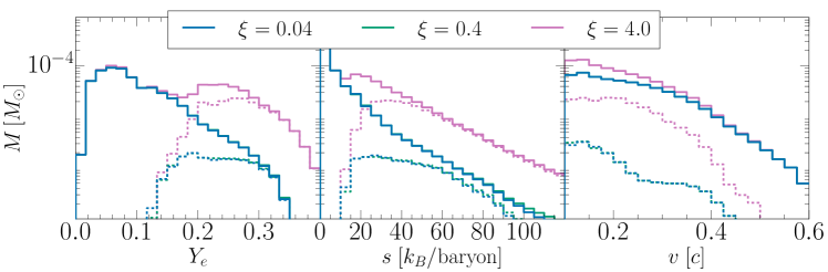
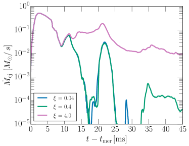
We can also quantify the nuclear composition of the outflow. We do so by tracking the electron fraction at large distances. Previous numerical studies have suggested that magnetically driven polar outflows may be required to provide additional protons necessary to match observed kilonova afterglows [23, 25, 24], (but see also, e.g., Ref. [125], for disk models). In Fig. 9, we depict the nuclear composition in terms of the proton fraction . We can see that the low magnetization case () does not feature any enhancement of . On the other hand the cases that do feature break-out of the field drive midly relativistic outflows, and especially the simulation with features substantial proton-rich winds coming from the star, albeit with only very mildly relativistic velocities. We can also provide a more quantitative assessment of the properties of these outflows. In Fig. 10, we show the compositional and entropy properties of the flows. We confirm the presence of a second peak around in addition to the bulk of the dynamical ejecta, which are very neutron rich . Similarly, the ejecta have significantly higher entropy when the dynamo action leads to the launching of mildly relativistic mass ejection. These results are roughly consistent with previous studies that only used neutrino cooling [23], but are lower than what would be expected for polar outflows when neutrino absorption was included [39, 24]. We can finally comment on the mass flux of the ejecta ( Fig. 12). After the dynamical ejecta have propagated out (), we can see the presence of a sustained outflow for dynamo parameters supporting magnetically driven polar outflows. In the case of strong amplification (), we find a sustained quasi-steady outflow rate, which is slightly lower than the dynamical mass ejection rate, for the dynamo parameters . This steady-state outflow rate is in good agreement with recent simulations in full numerical relativity [25]. Our results then indicate that – if these rates were sustained – strong dynamo amplification in the surface layer of the star may be needed to drive sustained outflows. It is important to mention that the main purpose of these simulations is to perform a first evaluation of the subgrid dynamo model presented in Sec. II. We therefore consider only short simulations , over which secular mass ejection driven largely by the disk has not yet fully set in. However, secular mass ejection is likely to dominate the total amount of ejecta [105]. In the case of a purely viscously driven evolution, mass ejection from the star has been shown to be variable at late times [19, 126].
IV Conclusions
We have investigated the impact of an -dynamo in a magnetar remnant formed in a binary neutron star merger. This was done using a new approach to the dynamo mean field equations in GRMHD, which resembles the Newtonian formulation of the equations. Based on heuristically motivated closure relations for an MRI-unstable layer in the HMNS, we have performed several simulations varying the degree of dynamo saturation in the star. We find that for strong amplification in excess of a magnetization , magnetic winding will generate strong toroidal fields, leading to an eventual magneto-bouyant break out of the field lines from the star by means of a Parker instability [110, 28]. This is consistent with previous work [52, 25, 33] showing that these field lines will then rearrange into a magnetic tower configuration [117], which may power intermittent outflows [33]. We find that in the case of sufficient dynamo amplification, these will be preceded by a short period of flares [52], which may be able to power a short gamma-ray burst precursor [8]. Crucially, we find that for strong amplification the Poynting flux can reach , while for a weaker dynamo strength it will never exceed . Higher dynamo amplification than considered in this work would likely drive stronger Poynting fluxes. Similarly, we find that the terminal Lorentz factor of the magnetically driven winds as well as the degree of proton-richness of the outflows correlate strongly with the dynamo amplification. We caution that the results may be strongly affected by the degree of baryon loading, which in our simulations will be underestimated due to the lack of neutrino absorption in the simulation [39, 124]. Clarifying this point will require simulations using full neutrino transport of the postmerger remnant [34, 24]. Overall, the picture we find for strong dynamo amplification, however, appears qualitatively consistent with recent works in the literature [23, 25, 24], even though our electromagnetic fluxes appear to be lower. To fully determine the realistic amount of dynamo amplification as well as performing a calibration of the subgrid model proposed here will require high-resolution simulations able to self-consistently capture the precise amount of amplification present in the system [33, 97, 30]. This leads us to conclude in line with recent very high-resolution simulations of the dynamo, that strong magnetic field amplification in the outer layers of the star may be an important ingredient for our understanding of whether magnetar remnants can power gamma-ray bursts.
Acknowledgments
The author gratefully acknowledges insightful discussions with A. Beloborodov, A. Bhattacharjee, L. Combi, P. Mösta, C. Musolino, L. Rezzolla, and E. Quataert. This work is supported by the National Science Foundation under grant No. PHY-2309210. This work mainly used Delta at the National Center for Supercomputing Applications (NCSA) through allocation PHY210074 from the Advanced Cyberinfrastructure Coordination Ecosystem: Services & Support (ACCESS) program, which is supported by National Science Foundation grants #2138259, #2138286, #2138307, #2137603, and #2138296. Additional simulations were performed on the NSF Frontera supercomputer under grant AST21006. We acknowledge the use of the following software packages: EinsteinToolkit [100], FUKA [102], Kadath [103], kuibit [127], matplotlib [128], numpy [129], scipy [130].
Appendix A Turbulent kinetic energy estimate
Here we want to provide some details on the turbulent kinetic energy saturation criterion used in Sec. II.3. Specifically, we adopt the approach of Refs. [78, 79, 80, 81] to model a proxy for the turbulent kinetic energy in the implicit large eddy paradigm, i.e., without including explicit viscous and resistive scales. Rather than adopting a full closure model [131, 132], our aim is to provide a simple way of incorporating a mean field dynamo effect, which does not compromise the stability of current GRMHD codes [92, 61]. As a starting point, we assume that the turbulent energy in the implicit large-eddy approach can be related to the square of the shear tensor, [78]. Using the formalism of dissipative hydrodynamics [133], one can write the entropy current for a flow exhibiting shear stresses and resistive dissipation, as
| (38) |
where is the fluid temperature, and the terms on the right correspond to viscous and resistive heating, respectively. Here, are the electric current and is the covariant shear tensor. While viscous stresses vanish for a perfect fluid, we can easily clarify that the dynamo model proposed here does not contribute to entropy production at the expansion order considered. For simplicity we assume , where is the effective (numerical resisitvity). Since then ,the entropy density is conserved up to the validity of our dynamo approximation,
| (39) |
In line with Refs. [78, 79], we now need to identify an effective turbulent kinetic energy, associated with the turbulent kinetic energy budget available. Due to the similarities of the Newtonian equations with Eq. (38), we heuristically propose
| (40) |
Note that is not conserved and decays on a timescale, , consistent with the effective turbulent energy cascade. In turn, is a new free parameter of this system.
In practice, on macroscopic (slow) timescales the system will likely approach a steady state equilibrium, between driving and decay of turbulence. In this case, the system relaxes such that . This leads to a steady state turbulent kinetic energy
| (41) |
For the application considered here, we can correlate the turbulent viscosity with a mixing length, [134, 83]. On dimensional grounds we may write , where is the characteristic speed of the medium corresponding to the sound speed, , in hydrodynamic turbulence, or to the Alfven speed for Alfvenic turbulence. Due to the steady state approximation, we further make the assumption that the turbulent decay timescale .
Following Ref. [79], we now assume that the turbulently driven dynamo action is quenched, when the magnetic energy density reaches a critical fraction of the turbulent energy budget, . Put differently, saturation should set in when a target magnetization is reached. In summary, this leads to an effective magnetization set by turbulence as
| (42) |
where for convenience we have absorbed the remaining constant numerical prefactor into .
References
- Baiotti and Rezzolla [2017] L. Baiotti and L. Rezzolla, Binary neutron star mergers: a review of Einstein’s richest laboratory, Rept. Prog. Phys. 80, 096901 (2017), arXiv:1607.03540 [gr-qc] .
- Metzger [2020] B. D. Metzger, Kilonovae, Living Rev. Rel. 23, 1 (2020), arXiv:1910.01617 [astro-ph.HE] .
- Ruiz et al. [2021] M. Ruiz, S. L. Shapiro, and A. Tsokaros, Multimessenger Binary Mergers Containing Neutron Stars: Gravitational Waves, Jets, and -Ray Bursts, Front. Astron. Space Sci. 8, 39 (2021), arXiv:2102.03366 [astro-ph.HE] .
- Abbott et al. [2017] B. P. Abbott et al. (LIGO Scientific, Virgo, Fermi GBM, INTEGRAL, IceCube, AstroSat Cadmium Zinc Telluride Imager Team, IPN, Insight-Hxmt, ANTARES, Swift, AGILE Team, 1M2H Team, Dark Energy Camera GW-EM, DES, DLT40, GRAWITA, Fermi-LAT, ATCA, ASKAP, Las Cumbres Observatory Group, OzGrav, DWF (Deeper Wider Faster Program), AST3, CAASTRO, VINROUGE, MASTER, J-GEM, GROWTH, JAGWAR, CaltechNRAO, TTU-NRAO, NuSTAR, Pan-STARRS, MAXI Team, TZAC Consortium, KU, Nordic Optical Telescope, ePESSTO, GROND, Texas Tech University, SALT Group, TOROS, BOOTES, MWA, CALET, IKI-GW Follow-up, H.E.S.S., LOFAR, LWA, HAWC, Pierre Auger, ALMA, Euro VLBI Team, Pi of Sky, Chandra Team at McGill University, DFN, ATLAS Telescopes, High Time Resolution Universe Survey, RIMAS, RATIR, SKA South Africa/MeerKAT), Multi-messenger Observations of a Binary Neutron Star Merger, Astrophys. J. Lett. 848, L12 (2017), arXiv:1710.05833 [astro-ph.HE] .
- Gottlieb et al. [2023a] O. Gottlieb et al., Large-scale Evolution of Seconds-long Relativistic Jets from Black Hole–Neutron Star Mergers, Astrophys. J. Lett. 954, L21 (2023a), arXiv:2306.14947 [astro-ph.HE] .
- Hayashi et al. [2022] K. Hayashi, S. Fujibayashi, K. Kiuchi, K. Kyutoku, Y. Sekiguchi, and M. Shibata, General-relativistic neutrino-radiation magnetohydrodynamic simulation of seconds-long black hole-neutron star mergers, Phys. Rev. D 106, 023008 (2022), arXiv:2111.04621 [astro-ph.HE] .
- Hayashi et al. [2023] K. Hayashi, K. Kiuchi, K. Kyutoku, Y. Sekiguchi, and M. Shibata, General-relativistic neutrino-radiation magnetohydrodynamics simulation of seconds-long black hole-neutron star mergers: Dependence on the initial magnetic field strength, configuration, and neutron-star equation of state, Phys. Rev. D 107, 123001 (2023), arXiv:2211.07158 [astro-ph.HE] .
- Gottlieb et al. [2023b] O. Gottlieb, B. D. Metzger, E. Quataert, D. Issa, and F. Foucart, A Unified Picture of Short and Long Gamma-ray Bursts from Compact Binary Mergers, (2023b), arXiv:2309.00038 [astro-ph.HE] .
- Etienne et al. [2012a] Z. B. Etienne, Y. T. Liu, V. Paschalidis, and S. L. Shapiro, General relativistic simulations of black hole-neutron star mergers: Effects of magnetic fields, Phys. Rev. D 85, 064029 (2012a), arXiv:1112.0568 [astro-ph.HE] .
- Etienne et al. [2012b] Z. B. Etienne, V. Paschalidis, and S. L. Shapiro, General relativistic simulations of black hole-neutron star mergers: Effects of tilted magnetic fields, Phys. Rev. D 86, 084026 (2012b), arXiv:1209.1632 [astro-ph.HE] .
- Ruiz et al. [2020] M. Ruiz, A. Tsokaros, and S. L. Shapiro, Magnetohydrodynamic Simulations of Binary Neutron Star Mergers in General Relativity: Effects of Magnetic Field Orientation on Jet Launching, Phys. Rev. D 101, 064042 (2020), arXiv:2001.09153 [astro-ph.HE] .
- Most et al. [2021] E. R. Most, L. J. Papenfort, S. D. Tootle, and L. Rezzolla, On accretion discs formed in MHD simulations of black hole–neutron star mergers with accurate microphysics, Mon. Not. Roy. Astron. Soc. 506, 3511 (2021), arXiv:2106.06391 [astro-ph.HE] .
- Paschalidis et al. [2015] V. Paschalidis, M. Ruiz, and S. L. Shapiro, Relativistic Simulations of Black Hole–neutron Star Coalescence: the jet Emerges, Astrophys. J. Lett. 806, L14 (2015), arXiv:1410.7392 [astro-ph.HE] .
- Paschalidis et al. [2013] V. Paschalidis, Z. B. Etienne, and S. L. Shapiro, General relativistic simulations of binary black hole-neutron stars: Precursor electromagnetic signals, Phys. Rev. D 88, 021504 (2013), arXiv:1304.1805 [astro-ph.HE] .
- East et al. [2021] W. E. East, L. Lehner, S. L. Liebling, and C. Palenzuela, Multimessenger Signals from Black Hole–Neutron Star Mergers without Significant Tidal Disruption, Astrophys. J. Lett. 912, L18 (2021), arXiv:2101.12214 [astro-ph.HE] .
- Carrasco et al. [2021] F. Carrasco, M. Shibata, and O. Reula, Magnetospheres of black hole-neutron star binaries, Phys. Rev. D 104, 063004 (2021), arXiv:2106.09081 [astro-ph.HE] .
- Most and Philippov [2023] E. R. Most and A. A. Philippov, Electromagnetic Precursors to Black Hole–Neutron Star Gravitational Wave Events: Flares and Reconnection-powered Fast Radio Transients from the Late Inspiral, Astrophys. J. Lett. 956, L33 (2023), arXiv:2309.04271 [astro-ph.HE] .
- Metzger and Fernández [2014] B. D. Metzger and R. Fernández, Red or blue? A potential kilonova imprint of the delay until black hole formation following a neutron star merger, Mon. Not. Roy. Astron. Soc. 441, 3444 (2014), arXiv:1402.4803 [astro-ph.HE] .
- Fujibayashi et al. [2018] S. Fujibayashi, K. Kiuchi, N. Nishimura, Y. Sekiguchi, and M. Shibata, Mass Ejection from the Remnant of a Binary Neutron Star Merger: Viscous-Radiation Hydrodynamics Study, Astrophys. J. 860, 64 (2018), arXiv:1711.02093 [astro-ph.HE] .
- Fahlman and Fernández [2018] S. Fahlman and R. Fernández, Hypermassive Neutron Star Disk Outflows and Blue Kilonovae, Astrophys. J. Lett. 869, L3 (2018), arXiv:1811.08906 [astro-ph.HE] .
- Metzger et al. [2018] B. D. Metzger, T. A. Thompson, and E. Quataert, A magnetar origin for the kilonova ejecta in GW170817, Astrophys. J. 856, 101 (2018), arXiv:1801.04286 [astro-ph.HE] .
- Kawaguchi et al. [2022] K. Kawaguchi, S. Fujibayashi, K. Hotokezaka, M. Shibata, and S. Wanajo, Electromagnetic Counterparts of Binary-neutron-star Mergers Leading to a Strongly Magnetized Long-lived Remnant Neutron Star, Astrophys. J. 933, 22 (2022), arXiv:2202.13149 [astro-ph.HE] .
- Mösta et al. [2020] P. Mösta, D. Radice, R. Haas, E. Schnetter, and S. Bernuzzi, A magnetar engine for short GRBs and kilonovae, Astrophys. J. Lett. 901, L37 (2020), arXiv:2003.06043 [astro-ph.HE] .
- Curtis et al. [2023] S. Curtis, P. Bosch, P. Mösta, D. Radice, S. Bernuzzi, A. Perego, R. Haas, and E. Schnetter, Outflows from Short-Lived Neutron-Star Merger Remnants Can Produce a Blue Kilonova, (2023), arXiv:2305.07738 [astro-ph.HE] .
- Combi and Siegel [2023] L. Combi and D. M. Siegel, Jets from neutron-star merger remnants and massive blue kilonovae, (2023), arXiv:2303.12284 [astro-ph.HE] .
- Price and Rosswog [2006] D. Price and S. Rosswog, Producing ultra-strong magnetic fields in neutron star mergers, Science 312, 719 (2006), arXiv:astro-ph/0603845 .
- Kiuchi et al. [2015] K. Kiuchi, P. Cerdá-Durán, K. Kyutoku, Y. Sekiguchi, and M. Shibata, Efficient magnetic-field amplification due to the Kelvin-Helmholtz instability in binary neutron star mergers, Phys. Rev. D 92, 124034 (2015), arXiv:1509.09205 [astro-ph.HE] .
- Kiuchi et al. [2018] K. Kiuchi, K. Kyutoku, Y. Sekiguchi, and M. Shibata, Global simulations of strongly magnetized remnant massive neutron stars formed in binary neutron star mergers, Phys. Rev. D 97, 124039 (2018), arXiv:1710.01311 [astro-ph.HE] .
- Aguilera-Miret et al. [2022] R. Aguilera-Miret, D. Viganò, and C. Palenzuela, Universality of the Turbulent Magnetic Field in Hypermassive Neutron Stars Produced by Binary Mergers, Astrophys. J. Lett. 926, L31 (2022), arXiv:2112.08406 [gr-qc] .
- Aguilera-Miret et al. [2023] R. Aguilera-Miret, C. Palenzuela, F. Carrasco, and D. Viganò, The role of turbulence and winding in the development of large-scale, strong magnetic fields in long-lived remnants of binary neutron star mergers, (2023), arXiv:2307.04837 [astro-ph.HE] .
- Skoutnev et al. [2021] V. Skoutnev, E. R. Most, A. Bhattacharjee, and A. A. Philippov, Scaling of Small-scale Dynamo Properties in the Rayleigh–Taylor Instability, Astrophys. J. 921, 75 (2021), arXiv:2106.04787 [physics.flu-dyn] .
- Balbus and Hawley [1991] S. A. Balbus and J. F. Hawley, A powerful local shear instability in weakly magnetized disks. 1. Linear analysis. 2. Nonlinear evolution, Astrophys. J. 376, 214 (1991).
- Kiuchi et al. [2023] K. Kiuchi, A. Reboul-Salze, M. Shibata, and Y. Sekiguchi, A large-scale magnetic field via dynamo in binary neutron star mergers, (2023), arXiv:2306.15721 [astro-ph.HE] .
- Radice and Bernuzzi [2023a] D. Radice and S. Bernuzzi, Ab-Initio General-Relativistic Neutrino-Radiation Hydrodynamics Simulations of Long-Lived Neutron Star Merger Remnants to Neutrino Cooling Timescales, (2023a), arXiv:2306.13709 [astro-ph.HE] .
- Guilet et al. [2017] J. Guilet, A. Bauswein, O. Just, and H.-T. Janka, Magnetorotational instability in neutron star mergers: impact of neutrinos, Mon. Not. Roy. Astron. Soc. 471, 1879 (2017), arXiv:1610.08532 [astro-ph.HE] .
- Liska et al. [2020] M. T. P. Liska, A. Tchekhovskoy, and E. Quataert, Large-Scale Poloidal Magnetic Field Dynamo Leads to Powerful Jets in GRMHD Simulations of Black Hole Accretion with Toroidal Field, Mon. Not. Roy. Astron. Soc. 494, 3656 (2020), arXiv:1809.04608 [astro-ph.HE] .
- Christie et al. [2019] I. M. Christie, A. Lalakos, A. Tchekhovskoy, R. Fernández, F. Foucart, E. Quataert, and D. Kasen, The Role of Magnetic Field Geometry in the Evolution of Neutron Star Merger Accretion Discs, Mon. Not. Roy. Astron. Soc. 490, 4811 (2019), arXiv:1907.02079 [astro-ph.HE] .
- Jacquemin-Ide et al. [2023] J. Jacquemin-Ide, F. Rincon, A. Tchekhovskoy, and M. Liska, Magnetorotational dynamo can generate large-scale vertical magnetic fields in 3D GRMHD simulations of accreting black holes, (2023), arXiv:2311.00034 [astro-ph.HE] .
- Dessart et al. [2009] L. Dessart, C. D. Ott, A. Burrows, S. Rosswog, and E. Livne, Neutrino signatures and the neutrino-driven wind in Binary Neutron Star Mergers, Astrophys. J. 690, 1681 (2009), arXiv:0806.4380 [astro-ph] .
- Giacomazzo et al. [2015] B. Giacomazzo, J. Zrake, P. Duffell, A. I. MacFadyen, and R. Perna, Producing Magnetar Magnetic Fields in the Merger of Binary Neutron Stars, Astrophys. J. 809, 39 (2015), arXiv:1410.0013 [astro-ph.HE] .
- Palenzuela et al. [2015] C. Palenzuela, S. L. Liebling, D. Neilsen, L. Lehner, O. L. Caballero, E. O’Connor, and M. Anderson, Effects of the microphysical Equation of State in the mergers of magnetized Neutron Stars With Neutrino Cooling, Phys. Rev. D 92, 044045 (2015), arXiv:1505.01607 [gr-qc] .
- Aguilera-Miret et al. [2020] R. Aguilera-Miret, D. Viganò, F. Carrasco, B. Miñano, and C. Palenzuela, Turbulent magnetic-field amplification in the first 10 milliseconds after a binary neutron star merger: Comparing high-resolution and large-eddy simulations, Phys. Rev. D 102, 103006 (2020), arXiv:2009.06669 [gr-qc] .
- Palenzuela et al. [2022] C. Palenzuela, R. Aguilera-Miret, F. Carrasco, R. Ciolfi, J. V. Kalinani, W. Kastaun, B. Miñano, and D. Viganò, Turbulent magnetic field amplification in binary neutron star mergers, Phys. Rev. D 106, 023013 (2022), arXiv:2112.08413 [gr-qc] .
- Bucciantini and Del Zanna [2013] N. Bucciantini and L. Del Zanna, A fully covariant mean-field dynamo closure for numerical 3+1 resistive GRMHD, Mon. Not. Roy. Astron. Soc. 428, 71 (2013), arXiv:1205.2951 [astro-ph.HE] .
- Sadowski et al. [2015] A. Sadowski, R. Narayan, A. Tchekhovskoy, D. Abarca, Y. Zhu, and J. C. McKinney, Global simulations of axisymmetric radiative black hole accretion discs in general relativity with a mean-field magnetic dynamo, Mon. Not. Roy. Astron. Soc. 447, 49 (2015), arXiv:1407.4421 [astro-ph.HE] .
- Tomei et al. [2020] N. Tomei, L. Del Zanna, M. Bugli, and N. Bucciantini, General relativistic magnetohydrodynamic dynamo in thick accretion discs: fully non-linear simulations, Mon. Not. Roy. Astron. Soc. 491, 2346 (2020), arXiv:1911.01838 [astro-ph.HE] .
- Shibata et al. [2021] M. Shibata, S. Fujibayashi, and Y. Sekiguchi, Long-term evolution of a merger-remnant neutron star in general relativistic magnetohydrodynamics: Effect of magnetic winding, Phys. Rev. D 103, 043022 (2021), arXiv:2102.01346 [astro-ph.HE] .
- Hanauske et al. [2017] M. Hanauske, K. Takami, L. Bovard, L. Rezzolla, J. A. Font, F. Galeazzi, and H. Stöcker, Rotational properties of hypermassive neutron stars from binary mergers, Phys. Rev. D 96, 043004 (2017), arXiv:1611.07152 [gr-qc] .
- Kastaun et al. [2016] W. Kastaun, R. Ciolfi, and B. Giacomazzo, Structure of Stable Binary Neutron Star Merger Remnants: a Case Study, Phys. Rev. D 94, 044060 (2016), arXiv:1607.02186 [astro-ph.HE] .
- Parker [1958] E. N. Parker, Dynamics of the Interplanetary Gas and Magnetic Fields, Astrophys. J. 128, 664 (1958).
- Moffatt [1978] H. K. Moffatt, Magnetic field generation in electrically conducting fluids (1978).
- Most and Quataert [2023] E. R. Most and E. Quataert, Flares, Jets, and Quasiperiodic Outbursts from Neutron Star Merger Remnants, Astrophys. J. Lett. 947, L15 (2023), arXiv:2303.08062 [astro-ph.HE] .
- Brandenburg et al. [2017] A. Brandenburg, J. Schober, I. Rogachevskii, T. Kahniashvili, A. Boyarsky, J. Frohlich, O. Ruchayskiy, and N. Kleeorin, The turbulent chiral-magnetic cascade in the early universe, Astrophys. J. Lett. 845, L21 (2017), arXiv:1707.03385 [astro-ph.CO] .
- Rieder and Teyssier [2017] M. Rieder and R. Teyssier, A small-scale dynamo in feedback-dominated galaxies – II. The saturation phase and the final magnetic configuration, Mon. Not. Roy. Astron. Soc. 471, 2674 (2017), arXiv:1704.05845 [astro-ph.GA] .
- White et al. [2022] C. J. White, A. Burrows, M. S. B. Coleman, and D. Vartanyan, On the Origin of Pulsar and Magnetar Magnetic Fields, Astrophys. J. 926, 111 (2022), arXiv:2111.01814 [astro-ph.HE] .
- Palenzuela et al. [2009] C. Palenzuela, L. Lehner, O. Reula, and L. Rezzolla, Beyond ideal MHD: towards a more realistic modeling of relativistic astrophysical plasmas, Mon. Not. Roy. Astron. Soc. 394, 1727 (2009), arXiv:0810.1838 [astro-ph] .
- Ripperda et al. [2019] B. Ripperda, F. Bacchini, O. Porth, E. R. Most, H. Olivares, A. Nathanail, L. Rezzolla, J. Teunissen, and R. Keppens, General relativistic resistive magnetohydrodynamics with robust primitive variable recovery for accretion disk simulations, Astrophys. J. Suppl. 244, 10 (2019), arXiv:1907.07197 [physics.comp-ph] .
- Schoepe et al. [2018] A. Schoepe, D. Hilditch, and M. Bugner, Revisiting Hyperbolicity of Relativistic Fluids, Phys. Rev. D 97, 123009 (2018), arXiv:1712.09837 [gr-qc] .
- Andersson et al. [2021] N. Andersson, I. Hawke, T. Celora, and G. L. Comer, The physics of non-ideal general relativistic magnetohydrodynamics, Mon. Not. Roy. Astron. Soc. 509, 3737 (2021), arXiv:2108.08732 [astro-ph.HE] .
- Most et al. [2022] E. R. Most, J. Noronha, and A. A. Philippov, Modelling general-relativistic plasmas with collisionless moments and dissipative two-fluid magnetohydrodynamics, Mon. Not. Roy. Astron. Soc. 514, 4989 (2022), arXiv:2111.05752 [astro-ph.HE] .
- Kalinani et al. [2022] J. V. Kalinani, R. Ciolfi, W. Kastaun, B. Giacomazzo, F. Cipolletta, and L. Ennoggi, Implementing a new recovery scheme for primitive variables in the general relativistic magnetohydrodynamic code Spritz, Phys. Rev. D 105, 103031 (2022), arXiv:2107.10620 [astro-ph.HE] .
- Duez et al. [2005] M. D. Duez, Y. T. Liu, S. L. Shapiro, and B. C. Stephens, Relativistic magnetohydrodynamics in dynamical spacetimes: Numerical methods and tests, Phys. Rev. D 72, 024028 (2005), arXiv:astro-ph/0503420 .
- Palenzuela [2013] C. Palenzuela, Modeling magnetized neutron stars using resistive MHD, Mon. Not. Roy. Astron. Soc. 431, 1853 (2013), arXiv:1212.0130 [astro-ph.HE] .
- Dionysopoulou et al. [2013] K. Dionysopoulou, D. Alic, C. Palenzuela, L. Rezzolla, and B. Giacomazzo, General-Relativistic Resistive Magnetohydrodynamics in three dimensions: formulation and tests, Phys. Rev. D 88, 044020 (2013), arXiv:1208.3487 [gr-qc] .
- Qian et al. [2017] Q. Qian, C. Fendt, S. Noble, and M. Bugli, rHARM: Accretion and Ejection in Resistive GR-MHD, Astrophys. J. 834, 29 (2017), arXiv:1610.04445 [astro-ph.HE] .
- Harutyunyan et al. [2018] A. Harutyunyan, A. Nathanail, L. Rezzolla, and A. Sedrakian, Electrical Resistivity and Hall Effect in Binary Neutron-Star Mergers, Eur. Phys. J. A 54, 191 (2018), arXiv:1803.09215 [astro-ph.HE] .
- Brandenburg and Subramanian [2005] A. Brandenburg and K. Subramanian, Astrophysical magnetic fields and nonlinear dynamo theory, Phys. Rept. 417, 1 (2005), arXiv:astro-ph/0405052 .
- Sturrock [1994] P. A. Sturrock, Plasma physics: an introduction to the theory of astrophysical, geophysical and laboratory plasmas (Cambridge University Press, 1994).
- Gruzinov and Diamond [1994] A. V. Gruzinov and P. H. Diamond, Self-consistent theory of mean-field electrodynamics, Phys. Rev. Lett. 72, 1651 (1994).
- Gressel and Pessah [2015] O. Gressel and M. E. Pessah, Characterizing the mean-field dynamo in turbulent accretion disks, Astrophys. J. 810, 59 (2015), arXiv:1507.08634 [astro-ph.HE] .
- Armas and Camilloni [2022] J. Armas and F. Camilloni, A stable and causal model of magnetohydrodynamics, JCAP 10, 039, arXiv:2201.06847 [hep-th] .
- Pareschi and Russo [2005] L. Pareschi and G. Russo, Implicit–explicit runge–kutta schemes and applications to hyperbolic systems with relaxation, Journal of Scientific Computing 25, 129 (2005).
- Squire and Bhattacharjee [2015] J. Squire and A. Bhattacharjee, Generation of large-scale magnetic fields by small-scale dynamo in shear flows, Phys. Rev. Lett. 115, 175003 (2015), arXiv:1506.04109 [astro-ph.SR] .
- Arnowitt et al. [2008] R. L. Arnowitt, S. Deser, and C. W. Misner, The Dynamics of general relativity, Gen. Rel. Grav. 40, 1997 (2008), arXiv:gr-qc/0405109 .
- Hogg and Reynolds [2018] J. D. Hogg and C. Reynolds, The influence of accretion disk thickness on the large-scale magnetic dynamo, Astrophys. J. 861, 24 (2018), arXiv:1805.05372 [astro-ph.HE] .
- Most and Noronha [2021] E. R. Most and J. Noronha, Dissipative magnetohydrodynamics for nonresistive relativistic plasmas: An implicit second-order flux-conservative formulation with stiff relaxation, Phys. Rev. D 104, 103028 (2021), arXiv:2109.02796 [astro-ph.HE] .
- Gressel and Pessah [2022] O. Gressel and M. E. Pessah, Finite-time Response of Dynamo Mean-field Effects in Magnetorotational Turbulence, Astrophys. J. 928, 118 (2022), arXiv:2202.09272 [astro-ph.HE] .
- Schmidt and Federrath [2011] W. Schmidt and C. Federrath, A Fluid-Dynamical Subgrid Scale Model for Highly Compressible Astrophysical Turbulence, Astron. Astrophys. 528, A106 (2011), arXiv:1010.4492 [astro-ph.GA] .
- Liu et al. [2022] Y. Liu, M. Kretschmer, and R. Teyssier, A subgrid turbulent mean-field dynamo model for cosmological galaxy formation simulations, Mon. Not. Roy. Astron. Soc. 513, 6028 (2022), arXiv:2110.14246 [astro-ph.GA] .
- Miravet-Tenés et al. [2022] M. Miravet-Tenés, P. Cerdá-Durán, M. Obergaulinger, and J. A. Font, Assessment of a new sub-grid model for magnetohydrodynamical turbulence. I. Magnetorotational instability, Mon. Not. Roy. Astron. Soc. 517, 3505 (2022), arXiv:2210.02173 [astro-ph.HE] .
- Miravet-Tenés et al. [2023] M. Miravet-Tenés, P. Cerdá-Durán, M. Obergaulinger, and J. A. Font, Assessment of a new sub-grid model for magnetohydrodynamical turbulence. II. Kelvin-Helmholtz instability 10.1093/mnras/stad3237 (2023), arXiv:2308.06041 [astro-ph.HE] .
- Duez et al. [2006] M. D. Duez, Y. T. Liu, S. L. Shapiro, and M. Shibata, Evolution of magnetized, differentially rotating neutron stars: Simulations in full general relativity, Phys. Rev. D 73, 104015 (2006), arXiv:astro-ph/0605331 .
- Radice [2020] D. Radice, Binary Neutron Star Merger Simulations with a Calibrated Turbulence Model, Symmetry 12, 1249 (2020), arXiv:2005.09002 [astro-ph.HE] .
- Shapiro [2000] S. L. Shapiro, Differential rotation in neutron stars: Magnetic braking and viscous damping, Astrophys. J. 544, 397 (2000), arXiv:astro-ph/0010493 .
- Etienne et al. [2010] Z. B. Etienne, Y. T. Liu, and S. L. Shapiro, Relativistic magnetohydrodynamics in dynamical spacetimes: A new AMR implementation, Phys. Rev. D 82, 084031 (2010), arXiv:1007.2848 [astro-ph.HE] .
- Etienne et al. [2012c] Z. B. Etienne, V. Paschalidis, Y. T. Liu, and S. L. Shapiro, Relativistic MHD in dynamical spacetimes: Improved EM gauge condition for AMR grids, Phys. Rev. D 85, 024013 (2012c), arXiv:1110.4633 [astro-ph.HE] .
- Del Zanna et al. [2003] L. Del Zanna, N. Bucciantini, and P. Londrillo, An efficient shock-capturing central-type scheme for multidimensional relativistic flows. 2. Magnetohydrodynamics, Astron. Astrophys. 400, 397 (2003), arXiv:astro-ph/0210618 .
- Londrillo and Del Zanna [2004] P. Londrillo and L. Del Zanna, On the divergence-free condition in godunov-type schemes for ideal magnetohydrodynamics: the upwind constrained transport method, J. Comput. Phys. 195, 17 (2004), arXiv:astro-ph/0310183 .
- Del Zanna et al. [2007] L. Del Zanna, O. Zanotti, N. Bucciantini, and P. Londrillo, ECHO: an Eulerian Conservative High Order scheme for general relativistic magnetohydrodynamics and magnetodynamics, Astron. Astrophys. 473, 11 (2007), arXiv:0704.3206 [astro-ph] .
- Mignone et al. [2019] A. Mignone, G. Mattia, G. Bodo, and L. Del Zanna, A Constrained Transport Method for the Solution of the Resistive Relativistic MHD Equations, Mon. Not. Roy. Astron. Soc. 486, 4252 (2019), arXiv:1904.01530 [physics.comp-ph] .
- Noble et al. [2006] S. C. Noble, C. F. Gammie, J. C. McKinney, and L. Del Zanna, Primitive variable solvers for conservative general relativistic magnetohydrodynamics, Astrophys. J. 641, 626 (2006), arXiv:astro-ph/0512420 .
- Kastaun et al. [2021] W. Kastaun, J. V. Kalinani, and R. Ciolfi, Robust Recovery of Primitive Variables in Relativistic Ideal Magnetohydrodynamics, Phys. Rev. D 103, 023018 (2021), arXiv:2005.01821 [gr-qc] .
- Most et al. [2019] E. R. Most, L. J. Papenfort, and L. Rezzolla, Beyond second-order convergence in simulations of magnetized binary neutron stars with realistic microphysics, Mon. Not. Roy. Astron. Soc. 490, 3588 (2019), arXiv:1907.10328 [astro-ph.HE] .
- Etienne et al. [2015] Z. B. Etienne, V. Paschalidis, R. Haas, P. Mösta, and S. L. Shapiro, IllinoisGRMHD: An Open-Source, User-Friendly GRMHD Code for Dynamical Spacetimes, Class. Quant. Grav. 32, 175009 (2015), arXiv:1501.07276 [astro-ph.HE] .
- Borges et al. [2008] R. Borges, M. Carmona, B. Costa, and W. Don, An improved weighted essentially non-oscillatory scheme for hyperbolic conservation laws, Journal of Computational Physics 227, 3191 (2008).
- Harten et al. [1983] A. Harten, P. D. Lax, and B. v. Leer, On upstream differencing and godunov-type schemes for hyperbolic conservation laws, SIAM review 25, 35 (1983).
- Chabanov et al. [2023] M. Chabanov, S. D. Tootle, E. R. Most, and L. Rezzolla, Crustal Magnetic Fields Do Not Lead to Large Magnetic-field Amplifications in Binary Neutron Star Mergers, Astrophys. J. Lett. 945, L14 (2023), arXiv:2211.13661 [astro-ph.HE] .
- Bernuzzi and Hilditch [2010] S. Bernuzzi and D. Hilditch, Constraint violation in free evolution schemes: Comparing BSSNOK with a conformal decomposition of Z4, Phys. Rev. D 81, 084003 (2010), arXiv:0912.2920 [gr-qc] .
- Hilditch et al. [2013] D. Hilditch, S. Bernuzzi, M. Thierfelder, Z. Cao, W. Tichy, and B. Bruegmann, Compact binary evolutions with the Z4c formulation, Phys. Rev. D 88, 084057 (2013), arXiv:1212.2901 [gr-qc] .
- Loffler et al. [2012] F. Loffler et al., The Einstein Toolkit: A Community Computational Infrastructure for Relativistic Astrophysics, Class. Quant. Grav. 29, 115001 (2012), arXiv:1111.3344 [gr-qc] .
- Schnetter et al. [2004] E. Schnetter, S. H. Hawley, and I. Hawke, Evolutions in 3-D numerical relativity using fixed mesh refinement, Class. Quant. Grav. 21, 1465 (2004), arXiv:gr-qc/0310042 .
- Papenfort et al. [2021] L. J. Papenfort, S. D. Tootle, P. Grandclément, E. R. Most, and L. Rezzolla, New public code for initial data of unequal-mass, spinning compact-object binaries, Phys. Rev. D 104, 024057 (2021), arXiv:2103.09911 [gr-qc] .
- Grandclement [2010] P. Grandclement, Kadath: A Spectral solver for theoretical physics, J. Comput. Phys. 229, 3334 (2010), arXiv:0909.1228 [gr-qc] .
- Hempel and Schaffner-Bielich [2010] M. Hempel and J. Schaffner-Bielich, Statistical Model for a Complete Supernova Equation of State, Nucl. Phys. A 837, 210 (2010), arXiv:0911.4073 [nucl-th] .
- Radice et al. [2020] D. Radice, S. Bernuzzi, and A. Perego, The Dynamics of Binary Neutron Star Mergers and GW170817, Ann. Rev. Nucl. Part. Sci. 70, 95 (2020), arXiv:2002.03863 [astro-ph.HE] .
- Ciolfi et al. [2017] R. Ciolfi, W. Kastaun, B. Giacomazzo, A. Endrizzi, D. M. Siegel, and R. Perna, General relativistic magnetohydrodynamic simulations of binary neutron star mergers forming a long-lived neutron star, Phys. Rev. D 95, 063016 (2017), arXiv:1701.08738 [astro-ph.HE] .
- Siegel et al. [2013] D. M. Siegel, R. Ciolfi, A. I. Harte, and L. Rezzolla, Magnetorotational instability in relativistic hypermassive neutron stars, Phys. Rev. D 87, 121302 (2013), arXiv:1302.4368 [gr-qc] .
- Nedora et al. [2019] V. Nedora, S. Bernuzzi, D. Radice, A. Perego, A. Endrizzi, and N. Ortiz, Spiral-wave wind for the blue kilonova, Astrophys. J. Lett. 886, L30 (2019), arXiv:1907.04872 [astro-ph.HE] .
- Radice and Bernuzzi [2023b] D. Radice and S. Bernuzzi, Secular Outflows from Long-Lived Neutron Star Merger Remnants, in 15th International Conference on Numerical Modeling of Space Plasma Flows (2023) arXiv:2310.09934 [astro-ph.HE] .
- Acheson and Gibbons [1978] D. J. Acheson and M. P. Gibbons, On the Instability of Toroidal Magnetic Fields and Differential Rotation in Stars, Philosophical Transactions of the Royal Society of London Series A 289, 459 (1978).
- Kiuchi et al. [2011] K. Kiuchi, S. Yoshida, and M. Shibata, Non-axisymmetric instabilities of neutron star with toroidal magnetic fields, Astron. Astrophys. 532, A30 (2011), arXiv:1104.5561 [astro-ph.HE] .
- Parfrey et al. [2013] K. Parfrey, A. M. Beloborodov, and L. Hui, Dynamics of Strongly Twisted Relativistic Magnetospheres, Astrophys. J. 774, 92 (2013), arXiv:1306.4335 [astro-ph.HE] .
- Carrasco et al. [2019] F. Carrasco, D. Viganò, C. Palenzuela, and J. A. Pons, Triggering magnetar outbursts in 3D force-free simulations, Mon. Not. Roy. Astron. Soc. 484, L124 (2019), arXiv:1901.08889 [astro-ph.HE] .
- Mahlmann et al. [2023] J. F. Mahlmann, A. A. Philippov, V. Mewes, B. Ripperda, E. R. Most, and L. Sironi, Three-dimensional Dynamics of Strongly Twisted Magnetar Magnetospheres: Kinking Flux Tubes and Global Eruptions, Astrophys. J. Lett. 947, L34 (2023), arXiv:2302.07273 [astro-ph.HE] .
- Most and Philippov [2020] E. R. Most and A. A. Philippov, Electromagnetic precursors to gravitational wave events: Numerical simulations of flaring in pre-merger binary neutron star magnetospheres, Astrophys. J. Lett. 893, L6 (2020), arXiv:2001.06037 [astro-ph.HE] .
- Most and Philippov [2022] E. R. Most and A. A. Philippov, Electromagnetic precursor flares from the late inspiral of neutron star binaries, Mon. Not. Roy. Astron. Soc. 515, 2710 (2022), arXiv:2205.09643 [astro-ph.HE] .
- Lynden-Bell [1996] D. Lynden-Bell, Magnetic collimation by accretion discs of quasars and stars, Mon. Not. Roy. Astron. Soc. 279, 389 (1996).
- Shibata et al. [2011] M. Shibata, Y. Suwa, K. Kiuchi, and K. Ioka, Afterglow of binary neutron star merger, Astrophys. J. Lett. 734, L36 (2011), arXiv:1105.3302 [astro-ph.HE] .
- Bromberg and Tchekhovskoy [2016] O. Bromberg and A. Tchekhovskoy, Relativistic MHD simulations of core-collapse GRB jets: 3D instabilities and magnetic dissipation, Mon. Not. Roy. Astron. Soc. 456, 1739 (2016), arXiv:1508.02721 [astro-ph.HE] .
- Narayan et al. [1992] R. Narayan, B. Paczynski, and T. Piran, Gamma-ray bursts as the death throes of massive binary stars, Astrophys. J. Lett. 395, L83 (1992), arXiv:astro-ph/9204001 .
- Just et al. [2016] O. Just, M. Obergaulinger, H. T. Janka, A. Bauswein, and N. Schwarz, Neutron-star merger ejecta as obstacles to neutrino-powered jets of gamma-ray bursts, Astrophys. J. Lett. 816, L30 (2016), arXiv:1510.04288 [astro-ph.HE] .
- Foucart et al. [2016] F. Foucart, E. O’Connor, L. Roberts, L. E. Kidder, H. P. Pfeiffer, and M. A. Scheel, Impact of an improved neutrino energy estimate on outflows in neutron star merger simulations, Phys. Rev. D 94, 123016 (2016), arXiv:1607.07450 [astro-ph.HE] .
- Fujibayashi et al. [2017] S. Fujibayashi, Y. Sekiguchi, K. Kiuchi, and M. Shibata, Properties of Neutrino-driven Ejecta from the Remnant of a Binary Neutron Star Merger: Pure Radiation Hydrodynamics Case, Astrophys. J. 846, 114 (2017), arXiv:1703.10191 [astro-ph.HE] .
- Foucart et al. [2018] F. Foucart, M. D. Duez, L. E. Kidder, R. Nguyen, H. P. Pfeiffer, and M. A. Scheel, Evaluating radiation transport errors in merger simulations using a Monte Carlo algorithm, Phys. Rev. D 98, 063007 (2018), arXiv:1806.02349 [astro-ph.HE] .
- Miller et al. [2019] J. M. Miller, B. R. Ryan, J. C. Dolence, A. Burrows, C. J. Fontes, C. L. Fryer, O. Korobkin, J. Lippuner, M. R. Mumpower, and R. T. Wollaeger, Full Transport Model of GW170817-Like Disk Produces a Blue Kilonova, Phys. Rev. D 100, 023008 (2019), arXiv:1905.07477 [astro-ph.HE] .
- Fahlman et al. [2023] S. Fahlman, R. Fernández, and S. Morsink, Secular outflows from 3D MHD hypermassive neutron star accretion disc systems, Mon. Not. Roy. Astron. Soc. 526, 952 (2023), arXiv:2308.16237 [astro-ph.HE] .
- Bozzola [2021] G. Bozzola, kuibit: Analyzing Einstein Toolkit simulations with Python, The Journal of Open Source Software 6, 3099 (2021), arXiv:2104.06376 [gr-qc] .
- Hunter [2007] J. D. Hunter, Matplotlib: A 2d graphics environment, Computing in Science & Engineering 9, 90 (2007).
- Harris et al. [2020] C. R. Harris, K. J. Millman, S. J. van der Walt, R. Gommers, P. Virtanen, D. Cournapeau, E. Wieser, J. Taylor, S. Berg, N. J. Smith, R. Kern, M. Picus, S. Hoyer, M. H. van Kerkwijk, M. Brett, A. Haldane, J. F. del Río, M. Wiebe, P. Peterson, P. Gérard-Marchant, K. Sheppard, T. Reddy, W. Weckesser, H. Abbasi, C. Gohlke, and T. E. Oliphant, Array programming with NumPy, Nature 585, 357 (2020).
- Virtanen et al. [2020] P. Virtanen, R. Gommers, T. E. Oliphant, M. Haberland, T. Reddy, D. Cournapeau, E. Burovski, P. Peterson, W. Weckesser, J. Bright, S. J. van der Walt, M. Brett, J. Wilson, K. J. Millman, N. Mayorov, A. R. J. Nelson, E. Jones, R. Kern, E. Larson, C. J. Carey, İ. Polat, Y. Feng, E. W. Moore, J. VanderPlas, D. Laxalde, J. Perktold, R. Cimrman, I. Henriksen, E. A. Quintero, C. R. Harris, A. M. Archibald, A. H. Ribeiro, F. Pedregosa, P. van Mulbregt, and SciPy 1.0 Contributors, SciPy 1.0: Fundamental Algorithms for Scientific Computing in Python, Nature Methods 17, 261 (2020).
- Carrasco et al. [2020] F. Carrasco, D. Viganò, and C. Palenzuela, Gradient subgrid-scale model for relativistic MHD large-eddy simulations, Phys. Rev. D 101, 063003 (2020), arXiv:1908.01419 [astro-ph.HE] .
- Viganò et al. [2020] D. Viganò, R. Aguilera-Miret, F. Carrasco, B. Miñano, and C. Palenzuela, General relativistic MHD large eddy simulations with gradient subgrid-scale model, Phys. Rev. D 101, 123019 (2020), arXiv:2004.00870 [gr-qc] .
- Denicol and Rischke [2022] G. S. Denicol and D. H. Rischke, Microscopic Foundations of Relativistic Fluid Dynamics (Springer, 2022).
- Radice [2017] D. Radice, General-Relativistic Large-Eddy Simulations of Binary Neutron Star Mergers, Astrophys. J. Lett. 838, L2 (2017), arXiv:1703.02046 [astro-ph.HE] .