Singular Legendrian unknot links and relative Ginzburg algebras

Abstract.

We associate to a quiver and a subquiver $(Q,F)$ a stopped Weinstein manifold $X$ whose Legendrian attaching link is a singular Legendrian unknot link $\varLambda$. We prove that the relative Ginzburg algebra of $(Q,F)$ is quasi-isomorphic to the Chekanov–Eliashberg dg-algebra of $\varLambda$. It follows that the Chekanov–Eliashberg dg-algebra of $\varLambda$ relative to its boundary dg-subalgebra, and the Orlov functor associated to the partially wrapped Fukaya category of $X$ both admit a strong relative smooth Calabi–Yau structure.

1. Introduction

Let $Q$ be a quiver and let $F\subset Q$ be a subquiver called the frozen subquiver. Let $Z_{0}(Q)$ denote the subcritical Weinstein manifold obtained by taking Weinstein connected sum of copies of $B^{2n}$ equipped with the standard Liouville form $\lambda=\frac{1}{2}\sum_{i=1}^{n}(x_{i}dy_{i}-y_{i}dx_{i})$ according to the arrows of $Q$. We define a singular Legendrian $\varLambda(Q,F)$ in the contact boundary of $Z_{0}(Q)$ by first taking a copy of the $(n-1)$-dimensional Legendrian unknot contained in a Darboux chart in the boundary of each copy of $B^{2n}$. For each arrow in $Q$ we push part of the Legendrian unknot associated to its tail through the Weinstein $1$-handle to the copy of $B^{2n}$ associated with the head of the arrow. If the arrow is non-frozen we make the two Legendrians link once and if the arrow is frozen we make the two Legendrians have a single transverse intersection point. The result is a singular Legendrian unknot link in the boundary of $Z_{0}(Q)$, see Figure 1. The pair $(Z_{0}(Q),\varLambda(Q,F))$ specifies a stopped Weinstein manifold $X(Q,F)$ by attaching top Weinstein handles to non-frozen components of $\varLambda(Q,F)$ and a stop to each frozen component

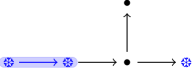
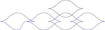
Figure 1. Left: A quiver $Q$ and frozen subquiver $F$ marked with blue snowflakes ❆ and blue arrows. Right: Front projection of corresponding singular Legendrian unknot link $\varLambda(Q,F)$ with frozen components marked in blue.

We let $CE^{\ast}(\varLambda(Q,F);Z_{0}(Q))$ denote the Chekanov–Eliashberg dg-algebra of $\varLambda(Q,F)$ over a field, which is defined as the Chekanov–Eliashberg dg-algebra after taking a Weinstein neighborhood of each frozen component of $\varLambda(Q,F)$, see [AE22, Section 3.1]. Let $\mathscr{G}^{\ast}_{n}(Q,F)$ denote the $n$-dimensional relative Ginzburg algebra of $(Q,F)$ (see 2.2).

Theorem 1.1.

Let $Q$ be a quiver and $F\subset Q$ a subquiver and let $n\geq 4$. There is a quasi-isomorphism of dg-algebras $CE^{\ast}(\varLambda(Q,F);Z_{0}(Q))\cong\mathscr{G}^{\ast}_{n}(Q,F)$. Furthermore, there is a dg-algebra $\mathcal{B}$ together with a canonical inclusion $\mathcal{B}\hookrightarrow CE^{\ast}(\varLambda(Q,F);Z_{0}(Q))$ and a quasi-isomorphism of dg-algebras $\mathcal{B}\cong\mathscr{G}^{\ast}_{n-1}(F)$.

Remark 1.2.

1. 1.1 also holds for $n=3$ if every vertex of $F$ has valency less than three.

2. If $F_{1}=\varnothing$, then $\mathcal{B}\cong C_{-\ast}(\varOmega\varLambda(F))$ where $\varLambda(F)\subset\varLambda(Q,F)$ is the Legendrian sublink consisting of the frozen components only, and the dg-algebra $CE^{\ast}(\varLambda(Q,F);Z_{0}(Q))$ is the Chekanov–Eliashberg dg-algebra of $\varLambda(Q,F)$ with loop space coefficients in $C_{-\ast}(\varOmega\varLambda(F))$ as defined by Ekholm–Lekili [EL17, Section 3.2].

Brav–Dyckerhoff introduced the notion of a (strong) relative Calabi–Yau structure [BD19], and in line with the terminology of Kontsevich–Soibelman [KS09], a smooth Calabi–Yau structure is a left Calabi–Yau structure in the terminology of Brav–Dyckerhoff. We call a relative smooth Calabi–Yau structure weak if the quasi-isomorphisms in [BD19, (1.13)] does not necessarily come from a class in relative negative cyclic homology.

The canonical inclusion $\mathscr{G}^{\ast}_{n-1}(F)\hookrightarrow\mathscr{G}^{\ast}_{n}(Q,F)$ (see 2.3) admits a strong relative smooth $n$-Calabi–Yau structure by 2.4. Hence we conclude the following.

Corollary 1.3.

The canonical inclusion map $\mathcal{B}\hookrightarrow CE^{\ast}(\varLambda(Q,F);Z_{0}(Q))$ admits a strong relative smooth $n$-Calabi–Yau structure.

It follows from the result [AE22, Theorem 1.1] that there is a derived equivalence

$$\operatorname{Perf}CE^{\ast}(\varLambda(Q,F);Z_{0}(Q))\cong\mathcal{W}(X(Q,F);V(Q,F)),$$

where $\mathcal{W}(X(Q,F))$ denotes the partially wrapped Fukaya category of $X(Q,F)$ stopped at the Weinstein hypersurface $V(Q,F)$ and where $\operatorname{Perf}$ denotes the category of perfect modules, see [Syl19a, GPS20]. The Orlov functor $\iota_{V(Q,F)}\colon\mathcal{W}(V(Q,F))\hookrightarrow\mathcal{W}(X(Q,F);V(Q,F))$ (see [Syl19b, Section 2.4] for the definition) fits in a commutative diagram

(1.1) $$\leavevmode\hbox to198.98pt{\vbox to48.87pt{\text{[drawing]}}}, {\operatorname{Perf}\mathcal{B}} {\operatorname{Perf}CE^{\ast}(\varLambda(Q,F);Z_{0}(Q))} {\mathcal{W}(V(Q,F))} {\mathcal{W}(X(Q,F);V(Q,F))} \scriptstyle{\cong} \scriptstyle{\cong} \scriptstyle{\iota_{V(Q,F)}} {\operatorname{Perf}\mathcal{B}} {\operatorname{Perf}CE^{\ast}(\varLambda(Q,F);Z_{0}(Q))} {\mathcal{W}(V(Q,F))} {\mathcal{W}(X(Q,F);V(Q,F))} \scriptstyle{\cong} \scriptstyle{\cong} \scriptstyle{\iota_{V(Q,F)}}$$

leading to the following.

Corollary 1.4.

The Orlov functor $\iota_{V(Q,F)}$ admits a strong relative smooth $n$-Calabi–Yau structure.

1.1. Related results

As far as we know, the novelty of 1.3 is the existence of a strong relative smooth Calabi–Yau structure. Quite a bit is known in the non-relative case or in the weak case, as we list below.

• In the non-relative case $F=\varnothing$ it abstractly follows from the Bourgeois–Ekholm–Eliashberg surgery isomorphism [BEE12, Ekh19] together with the construction of a strong smooth $n$-Calabi–Yau structure on the wrapped Fukaya category due to Ganatra [Gan12, Gan19, Theorem 1.3; Theorem 3].

• Another proof in the non-relative case $F=\varnothing$ goes via [Asp23, Corollary 4.16] and the fact that the (non-relative) Ginzburg algebra is a strong smooth $n$-Calabi–Yau algebra [Kel11, Theorem 6.3].

• Assume $Q=\bullet$, $F=\varnothing$ and let $\varLambda$ be a horizontally displaceable Legendrian sphere (not necessarily an unknot) in the contactization of a Liouville domain. Then Legout [Leg23] proved that the Chekanov–Eliashberg dg-algebra of $\varLambda$ admits a weak $n$-Calabi–Yau structure via an explicit geometric construction.

  If $\varLambda\subset{\mathbb{R}}^{3}$ is not necessarily an unknot, Chen [Che23] proves in upcoming work that the augmentation category $\operatorname{\mathcal{A}ug}_{-}(\varLambda;{\mathbb{Z}}_{2})$ defined by Bourgeois–Chantraine [BC14, Section 3.2] carries a strong proper 2-Calabi–Yau structure. In the terminology of Brav–Dyckerhoff [BD19] this is a right Calabi–Yau structure.

• Assume $Q=F=\bullet$, and let $\varLambda\subset{\mathbb{R}}^{3}$ not necessarily an unknot. In upcoming work by Ma–Sabloff [MS23] it is proven that the $A_{\infty}$-functor $\operatorname{\mathcal{A}ug}_{+}(\varLambda;{\mathbb{Z}}_{2})\to\mathcal{C}(\varLambda;{\mathbb{Z}}_{2})$ that is defined on morphisms as precomposition with the canonical inclusion $C_{-\ast}(\varOmega\varLambda)\hookrightarrow CE^{\ast}(\varLambda;C_{-\ast}(\varOmega\varLambda))$ carries a weak relative proper $2$-Calabi–Yau structure, where $\operatorname{\mathcal{A}ug}_{+}$ denotes the augmentation category as defined in [NRS⁺20, Section 4].

• For general subcritical Weinstein manifolds and for general Legendrian submanifolds, 1.3 is proven in the weak case by Dimitroglou Rizell–Legout via an explicit geometric construction in upcoming work [DRL23].

1.4 is not new, but our proof is. It follows in the general case of stopped Weinstein manifolds admitting a stable polarization (which is always true for $X(Q,F)$) by combining work of Shende–Takeda [ST16, Theorem 1.14] and Ganatra–Pardon–Shende [GPS18, Theorem 1.4].

1.2. Outline of the proof

The proof of 1.1 follows from a generalization of the computation in [Asp23, Section 4.3], where the Chekanov–Eliashberg dg-algebra of the Legendrian attaching link of a plumbing of copies of $T^{\ast}S^{n}$ for $n\geq 3$ was computed. This computation is recovered from the one in this paper by letting $F=\varnothing$. A rough sketch of the proof of 1.1 is as follows.

1. Find a $1$-dimensional simplicial decomposition of the subcritical Weinstein manifold $Z_{0}(Q)$ in the sense of [Asp23, Section 2.2.4].

2. Find a singular Legendrian $\boldsymbol{\varLambda}(Q,F)$ relative to the simplicial decomposition of $Z_{0}(Q)$ whose completion is the singular Legendrian $\varLambda(Q,F)$ (see [Asp23, Definitions 4.1 and 4.2]).

3. Compute the Chekanov–Eliashberg dg-algebra of each part of $\boldsymbol{\varLambda}(Q,F)$. Each such piece is either a Legendrian unknot with boundary, Legendrian Hopf link with boundary or two Legendrian unknots with a transverse intersection, with boundary.

4. Using the local computation and the gluing formula for singular Chekanov–Eliashberg dg-algebras [Asp22, Theorem 2.34] we recover $CE^{\ast}(\varLambda(Q,F);Z_{0}(Q))$ up to quasi-isomorphism.

5. Write down an explicit chain homotopy equivalence between the resulting Chekanov–Eliashberg dg-algebra and the relative Ginzburg algebra of $(Q,F)$.

1.3. Future directions

Even though the relative Ginzburg algebra is known to not be a strong smooth Calabi–Yau algebra, it is expected to admit a pre-Calabi–Yau structure in the sense of Kontsevich–Takeda–Vlassopoulos [KTV21]. This is consistent with the folklore conjecture that the partially wrapped Fukaya category should admit a pre-Calabi–Yau structure, which is motivated by work of Seidel [Sei12, Section 3.3]. In view of the surgery formula for partially wrapped Fukaya categories [AE22, Theorem 1.1] we thus have the following.

Conjecture 1.5.

The Chekanov–Eliashberg dg-algebra of a singular Legendrian submanifold in the boundary of a subcritical Weinstein manifold admits a geometrically defined pre-Calabi–Yau structure.

In upcoming work, Ng [Ng23] defines an $L_{\infty}$-structure on a commutative version of the Chekanov–Eliashberg dg-algebra of a Legendrian in ${\mathbb{R}}^{3}$ with loop space coefficients, which we expect to be a shadow of the conjectured pre-Calabi–Yau structure.

Throughout this paper, every quiver come equipped with the trivial potential. An interesting problem that we hope to return to in the future is realizing the Ginzburg algebra of any $(Q,F)$ equipped with a non-trivial potential as a Chekanov–Eliashberg dg-algebra. The only example of such known to date is due to Li [Li19, Theorem 1.2].

Acknowledgments

The author is grateful to Georgios Dimitroglou Rizell and Noémie Legout for helpful comments on a draft of this paper and for explaining their work in progress, Merlin Christ for his guidance in the literature on relative Ginzburg algebras, Lenhard Ng for sharing a draft of his upcoming work [Ng23], Joshua Sabloff for sharing his upcoming results with Jiajie Ma [MS23] and Zhenyi Chen for sharing his upcoming results [Che23]. The author was supported by the Knut and Alice Wallenberg Foundation.

2. Relative Ginzburg algebras

Let $\boldsymbol{k}$ be a field. Let $Q$ be a quiver (with trivial potential), and let $F\subset Q$ be a subquiver. Let $\overline{Q}_{n}(F)$ denote the graded quiver with vertex set $Q_{0}$ and arrows consisting of the three following kinds.

• An arrow $g\colon v\to w$ in degree $0$ for each $g\colon v\to w$ in $Q_{1}$.

• An arrow $g^{\ast}\colon w\to v$ in degree $2-n$ for each $g\colon v\to w$ in $Q_{1}\smallsetminus F_{1}$.

• An arrow $h_{v}\colon v\to v$ in degree $1-n$ for each $v\in Q_{0}\smallsetminus F_{0}$.

We will use the notation $\overline{Q}_{n}\mathrel{\mathop{\mathchar 58\relax}}=\overline{Q}_{n}(\varnothing)$ and

$$[x,y]^{A}_{v}\mathrel{\mathop{\mathchar 58\relax}}=\sum_{A\ni e\colon v\to\bullet}xy-\sum_{A\ni e\colon\bullet\to v}yx,$$

where $A\subset Q_{1}$ is a subset.

Definition 2.1 ($n$-dimensional Ginzburg algebra).

The $n$-dimensional Ginzburg algebra $\mathscr{G}^{\ast}_{n}(Q)$ of the quiver $Q$ is the path algebra of $\overline{Q}_{n}$ equipped with the differential $d$ given on arrows by

$$dg=dg^{\ast}=0,\quad dh_{v}=[g,g^{\ast}]^{Q_{1}}_{v},\quad v\in Q_{0},$$

and extended to the whole path algebra by linearity and the Leibniz rule.

Definition 2.2 ($n$-dimensional relative Ginzburg algebra).

The $n$-dimensional relative Ginzburg algebra $\mathscr{G}^{\ast}_{n}(Q,F)$ of the tuple $(Q,F)$ is the path algebra of $\overline{Q}_{n}(F)$ equipped with the differential $d$ given on arrows by

$$dg=dg^{\ast}=0,\quad dh_{v}=[g,g^{\ast}]^{Q_{1}\smallsetminus F_{1}}_{v},\quad v\in Q_{0}\smallsetminus F_{0},$$

and extended to the whole path algebra by linearity and the Leibniz rule.

Lemma 2.3.

There is a map of dg-algebras $G\colon\mathscr{G}^{\ast}_{n-1}(F)\to\mathscr{G}^{\ast}_{n}(Q,F)$ that is defined on generators as $g\mapsto g$, $g^{\ast}\mapsto 0$ and $h_{v}\mapsto[g,g^{\ast}]^{Q_{1}\smallsetminus F_{1}}_{v}$ and extended to the whole of $\mathscr{G}^{\ast}_{n-1}(F)$ by linearity and multiplicativity.

Proof.

This is immediate from the definitions. ∎

The following result seems well-known to experts and implicitly alluded to in [Wu23, Section 7.2] and [KW21, Section 8] but we did not find an explicit reference in the literature.

Lemma 2.4.

The dg-algebra map $G\colon\mathscr{G}^{\ast}_{n-1}(F)\to\mathscr{G}^{\ast}_{n}(Q,F)$ defined in 2.3 admits a strong relative smooth $n$-Calabi–Yau structure.

Proof.

It is well-known that $\mathscr{G}^{\ast}_{n-1}(F)\cong\varPi_{n}(\boldsymbol{k}F)$ by [Kel11, Theorem 6.3], where $\varPi_{n}(\boldsymbol{k}F)$ denotes the $n$-Calabi–Yau completion of the path algebra of $F$. Yeung defined the relative $n$-Calabi–Yau completion $\varPi_{n}(\boldsymbol{k}Q,\boldsymbol{k}F)$ in [Yeu16, Section 7], and Wu defined a reduced version $\varPi_{n}^{\text{red}}(\boldsymbol{k}Q,\boldsymbol{k}F)$ in [Wu23, Section 3.6], which is quasi-isomorphic to $\varPi_{n}(\boldsymbol{k}Q,\boldsymbol{k}F)$ by [Wu23, Proposition 3.18]. It was proven by Yeung [Yeu16, Theorem 7.1], Bozec–Calaque–Scherotzke [BCS20, Corollary 5.24] and Wu [Wu23, Proposition 3.18] that the inclusion $\varPi_{n}(\boldsymbol{k}F)\hookrightarrow\varPi_{n}(\boldsymbol{k}Q,\boldsymbol{k}F)$ admits a strong relative smooth $n$-Calabi–Yau structure.

Thus it suffices to show that $\varPi_{n}^{\text{red}}(\boldsymbol{k}Q,\boldsymbol{k}F)\cong\mathscr{G}_{n}^{\ast}(Q,F)$, which is well-known to experts. In the same way that the $n$-Calabi–Yau completion in [Kel11] is defined as the tensor algebra of a shift of the inverse dualizing bimodule, the relative $n$-Calabi–Yau completion is defined as the tensor algebra of a shift of the relative inverse dualizing bimodule. An explicit description of the reduced version is described in [Wu23, p. 37], and the underlying module is generated by the dual arrows $g^{\ast}$ in degree $2-n$ for every $g\in Q_{1}\smallsetminus F_{1}$ and loops $h_{v}$ in degree $1-n$ for every $v\in Q_{0}\smallsetminus F_{0}$. A similar description for $n=2$ is found in [BCS20, Section 5.3.2] but holds for general $n$ in a similar manner. This finishes the proof ∎

Remark 2.5.

The dg-algebra $\varPi_{n}(\boldsymbol{k}Q,\boldsymbol{k}F)$ was also defined in [KW21] under the name relative derived preprojective algebra.

3. Stopped Weinstein manifolds associated to a quiver and a frozen subquiver

3.1. Weinstein manifolds and stops

Let us briefly recall some basic geometric definitions.

Definition 3.1 (Weinstein hypersurface).

A Weinstein hypersurface is a Weinstein embedding $(V^{2n-2},\lambda|_{V})\hookrightarrow(X\smallsetminus\operatorname{Core}X,\lambda)$ such that the induced map $V\to\partial X$ is an embedding. We will denote Weinstein embeddings by $V\hookrightarrow\partial X$.

Definition 3.2 (Weinstein pair).

A Weinstein pair is a tuple $(X^{2n},V^{2n-2})$ consisting of a Weinstein manifold $X$ and a Weinstein hypersurface $V\hookrightarrow\partial X$.

Definition 3.3 (Stop associated to a Weinstein hypersurface).

Let $(X,V)$ be a Weinstein pair. The stop associated to the Weinstein hypersurface $V\hookrightarrow\partial X$ is the Weinstein cobordism $\sigma_{V}$ obtained by gluing the Weinstein cobordism $(V\times D_{\varepsilon}T^{\ast}\varDelta^{1},\lambda_{V}+2xdy+ydx)$ to ${\mathbb{R}}\times(V\times{\mathbb{R}})$ along $V\times(-\varepsilon,\varepsilon)\hookrightarrow\partial({\mathbb{R}}\times(V\times{\mathbb{R}}))$.

Definition 3.4 (Weinstein manifold stopped at a Weinstein hypersurface).

Let $(X,V)$ be a Weinstein pair. The Weinstein manifold $X$ stopped at $V$ is the Weinstein cobordism obtained by gluing $\sigma_{V}$ to $X$ along $V\times(-\varepsilon,\varepsilon)$.

Remark 3.5.

Note that our usage of the word “stop” deviates slightly from the original usage in [Syl19a]. Our usage of the word stop originates from its usage in [EL17, Asp21, AE22].

Definition 3.6 (Weinstein manifold stopped at a Legendrian submanifold).

Let $X$ be a Weinstein manifold and $\varLambda\subset\partial X$ a Legendrian submanifold. We define the Weinstein manifold $X$ stopped at $\varLambda$ to be the Weinstein manifold $X$ stopped at a Weinstein neighborhood $T^{\ast}\varLambda$ of $\varLambda$.

Definition 3.7 (Legendrian relative to Weinstein pair).

Let $(X,V)$ be a Weinstein pair. A Legendrian submanifold relative to $V$ is a Legendrian submanifold-with-boundary $\varLambda\subset\partial X$ such that $\partial\varLambda\subset\partial V$ is Legendrian.

3.2. A simplicial decomposition

Let $Q$ be a quiver and let $F\subset Q$ be a subquiver called the frozen subquiver. Recall the definition of the pair $(Z_{0}(Q),\varLambda(Q,F))$ in Section 1. We pick a Weinstein neighborhood of each frozen component of $\varLambda(Q,F)$ together with a handle decomposition that consists of one Weinstein $0$-handle per frozen vertex of the component and one Weinstein $1$-handle per frozen edge of the component. Then let $P_{0}(F)$ denote the union of the subcritical parts of each of these Weinstein neighborhoods. The purpose of this section now is to describe a simplicial decomposition of $(Z_{0}(Q),P_{0}(F))$ (see [Asp23, Definition 2.15]) and a Legendrian submanifold $\boldsymbol{\varLambda}(Q,F)$ relative to this simplicial decomposition (see [Asp22, Definition 2.29]). The construction closely follows [Asp23, Section 4.3].

Let $C$ be the graph that is obtained by taking the underlying graph of $Q$, and adding one extra vertex in the middle of each edge. For convenience, we consider a partition $C_{0}=V\cup F_{0}\cup E\cup F_{1}$ where $V$ corresponds to elements of $Q_{0}\smallsetminus F_{0}$ (non-frozen vertices) and $E$ corresponds to elements in $Q_{1}\smallsetminus F_{1}$. The set $E\cup F_{1}$ consists of the newly added vertices (edge vertices), see Figure 2.

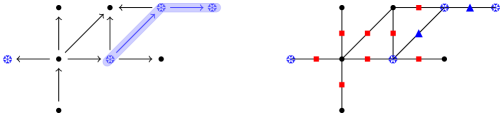
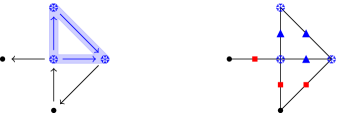
Figure 2. Left: Plumbing quivers $Q$ with a set $F_{0}$ of frozen vertices and a set $F_{1}$ of frozen edges. Right: The corresponding graph $C$ with vertex set $V\cup F_{0}\cup E\cup F_{1}$. The vertices represented by black dots $\bullet$ belong to $V$, the vertices represented by blue snowflakes ❆ belong to $F_{0}$, the vertices represented by red squares ${\color[rgb]{1,0,0}\blacksquare}$ belong to $E$ and the vertices represented by blue triangles ▲ belong to $F_{1}$.

A simplicial decomposition of $(Z_{0}(Q),P_{0}(F))$ is the tuple $((C,C^{\prime}),(\boldsymbol{V},\boldsymbol{V}^{\prime}))$ with $C$ as above and $C^{\prime}=F_{0}\cup F_{1}$ (where $F_{0}\cup F_{1}$ is viewed as a subset of the vertex set $C_{0}$). We call $e\in C_{1}$ a frozen edge if $e$ is adjacent to any frozen edge vertex. All other edges are called non-frozen.

Both $\boldsymbol{V}$ and $\boldsymbol{V}^{\prime}$ are sets consisting of Weinstein manifolds and Weinstein hypersurfaces of varying dimension. For simplicity we denote by $B^{2n}_{\text{std}}$ the Weinstein manifold consisting of $B^{2n}$ equipped with its standard Liouville one-form $\lambda=\frac{1}{2}\sum_{i=1}^{n}(x_{i}dy_{i}-y_{i}dx_{i})$. The set $\boldsymbol{V}$ consists of

1. one copy of $V^{2n-2}_{e}\mathrel{\mathop{\mathchar 58\relax}}=B^{2n-2}_{\text{std}}$ for each edge $e\in C_{1}$;

2. one copy of $V^{2n}_{v}\mathrel{\mathop{\mathchar 58\relax}}=B^{2n}_{\text{std}}$ for each vertex $v\in C_{0}$;

3. one Weinstein hypersurface $\iota_{v}\colon\bigsqcup_{C_{1}\ni e\supset v}V^{(1)}_{e}\hookrightarrow\partial V^{2n}_{v}$ for each vertex $v\in C_{0}$.

The set $\boldsymbol{V}^{\prime}$ consists of

1. one copy of $(V^{\prime})^{2n-2}_{v}\mathrel{\mathop{\mathchar 58\relax}}=B^{2n-2}_{\text{std}}$ for each frozen vertex and for each frozen edge vertex $v\in F_{0}\cup F_{1}\subset C_{0}$;

2. one copy of $(V^{\prime})^{2n-4}_{e}\mathrel{\mathop{\mathchar 58\relax}}=B^{2n-4}_{\text{std}}$ for each frozen edge $e\in F_{1}$;

3. one Weinstein hypersurface $\bigsqcup_{C_{1}\ni e\supset v}(V^{\prime})^{2n-4}_{e}\hookrightarrow\partial(V^{\prime})^{2n-2}_{v}$ for each frozen vertex $v\in F_{0}$ and frozen edge vertex $v\in F_{1}$.

We have that $(C,\boldsymbol{V})$ is a simplicial decomposition of $Z_{0}(Q)$, and $(C^{\prime},\boldsymbol{V}^{\prime})$ is a simplicial decomposition of $P_{0}$. To complete the construction, we have a hypersurface inclusion $(C^{\prime},\boldsymbol{V}^{\prime})\hookrightarrow(C,\boldsymbol{V})$ (see [Asp22, Definition 2.3]) which consists of

1. the inclusion $C^{\prime}=F\hookrightarrow C$ of the (underlying graph of the) frozen subquiver into $C$;

2. one Weinstein hypersurface $(V^{\prime})^{2n-4}_{e}\hookrightarrow V^{2n-2}_{e}$ for each edge $e\in C_{1}$;

3. one Weinstein hypersurface

   $$(V^{\prime})_{v}^{2n-2}\#_{(V^{\prime})_{e}^{2n-4}}V_{e}^{2n-2}\hookrightarrow\partial V_{v}^{2n}$$

   for each pair of a frozen (edge) vertex $v\in F_{0}\cup F_{1}$ and an edge $e\in C_{1}$ adjacent to $v$.

An example of the simplicial decomposition of $(Z_{0}(Q),P_{0}(F))$ is depicted in Figure 3.

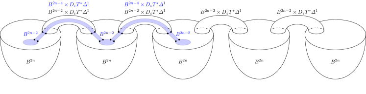
Figure 3. Top left: A quiver with a frozen subquiver $(Q,F)$. Top right: The simplicial complex $C$ associated to $(Q,F)$. Bottom: The simplicial decomposition of the pair $(Z_{0}(Q),P_{0}(F))$.

We now define a Legendrian submanifold relative to $((C^{\prime},C),(\boldsymbol{V},\boldsymbol{V}^{\prime}))$ denoted by $\boldsymbol{\varLambda}(Q,F)$ (see [Asp22, Definition 2.29]) as follows:

1. For each non-frozen edge vertex $v\in E$ let $\varLambda_{v}$ be the $(n-1)$-dimensional Hopf link $\varLambda_{1}\cup\varLambda_{2}$ with boundary such that $\partial\varLambda_{i}\subset\partial V^{2n-2}_{e_{i}}$ is the $(n-2)$-dimensional Legendrian unknot, where $e_{1},e_{2}\in C_{1}$ are the two edges adjacent to $v$, see Figure 4.

2. For each frozen edge vertex $v\in F_{1}$ let $\varLambda_{v}$ be two $(n-1)$-dimensional Legendrian disks $\varLambda_{1}\cup\varLambda_{2}$ with boundary in $\partial(V^{2n-2}_{e_{1}}\#_{(V^{\prime})^{2n-4}_{e_{1}}}(V^{\prime})^{2n-2}_{v}\#_{(V^{\prime})^{2n-4}_{e_{2}}}V^{2n-2}_{e_{2}})$ such that

   1. $\partial\varLambda_{i}\cap\partial V^{2n-2}_{e_{i}}\subset\partial V^{2n-2}_{e_{i}}$ is the $(n-2)$-dimensional Legendrian unknot with boundary a $(n-3)$-dimensional Legendrian unknot in $\partial(V^{\prime}){2n-2}_{e_{i}}$, where $e_{1},e_{2}\in C_{1}$ are the two edges adjacent to $v$, and

   2. $(\partial\varLambda_{1}\cup\partial\varLambda_{2})\cap\partial(V^{\prime})^{2n-2}_{v}\subset\partial(V^{\prime})^{2n-2}_{v}$ is the $(n-2)$-dimensional Hopf link with two boundary components, one in each $\partial(V^{\prime})^{2n-4}_{e_{i}}$ looking like the $(n-3)$-dimensional unknot, where $e_{1},e_{2}\in C_{1}$ are the two edges adjacent to $v$

   see Figure 5.

3. For each $v\in V$, let $\varLambda_{v}$ be the $(n-1)$-dimensional Legendrian unknot with $k$ open disks removed, where $k$ is the valency of the vertex $v$ such that each of the $k$ components of $\partial\varLambda_{v}$ is the $(n-2)$-dimensional Legendrian unknot in $\partial V^{2n-2}_{e_{i}}$ where $e_{1},\ldots,e_{k}\in C_{1}$ are the $k$ edges that are adjacent to $v$, see Figure 6.

4. For each $v\in F$, let $\varLambda_{v}$ is the $(n-1)$-dimensional Legendrian unknot with one boundary component being a $(n-2)$-dimensional Legendrian unknot in $\partial B^{2n-2}$ for each non-frozen edge adjacent to $v$.

   The new copy of $B^{2n-2}$ coming from the fact that $v\in F$ (see the definition of $\boldsymbol{V}^{\prime}$) is connected via a Weinstein $1$-handle to every other $B^{2n-2}$ corresponding to frozen edges of $C$ that are adjacent to $v$. The boundary $\varLambda_{v}$ in this new $B^{2n-2}$ is a $(n-2)$-dimensional unknot with some number of disks removed (corresponding to the number of frozen edges adjacent to $v$), see Figure 7.

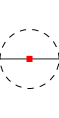
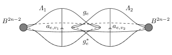
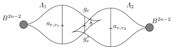
Figure 4. Top left: Local depiction of a vertex $v\in E$. Top right: Two copies of $B^{2n-2}$ with $\varLambda_{v}$ which becomes the $(n-1)$-dimensional Hopf link with boundary in $\partial(B^{2n-2}\sqcup B^{2n-2})$ after a small perturbation in a Darboux chart. Bottom: A slice of $\varLambda_{v}$ in generic position after a small perturbation, where the Reeb chords $g_{v}$ and $g_{v}^{\ast}$ are visible.

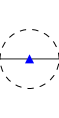
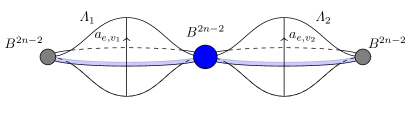
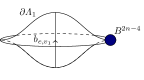
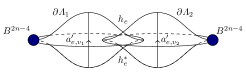
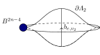
Figure 5. Top left: Local depiction of a vertex $v\in F_{1}$. Top right: Three copies of $B^{2n-2}$ with $\varLambda_{v}$ being two $(n-1)$-dimensional Legendrian disks with boundary in $\partial(B^{2n-2}\#_{B^{2n-4}}B^{2n-2}\#_{B^{2n-4}}B^{2n-2})$ in a Darboux chart. Bottom left: The boundary of $\varLambda_{1}$ in the leftmost copy of $B^{2n-2}$. Bottom middle: The boundary of $\varLambda_{1}\cup\varLambda_{2}$ in the middle blue copy of $B^{2n-2}$. Bottom right: The boundary of $\varLambda_{2}$ in the rightmost copy of $B^{2n-2}$.

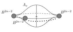
Figure 6. Left: Local depiction of a vertex $v\in V$ with valency $k$. Right: $k$ copies of $B^{2n-2}$ with $\varLambda_{v}$ being the $(n-1)$-dimensional Legendrian unknot with boundary in $\partial\left(\bigsqcup_{i=1}^{k}B^{2n-2}\right)$ in a Darboux chart.

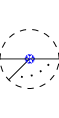
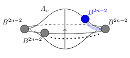
Figure 7. Left: Local depiction of a frozen vertex $v\in F$ with valency $k$. Right: $k+1$ copies of $B^{2n-2}$ with $\varLambda_{v}$ being the $(n-1)$-dimensional Legendrian unknot with boundary in $\partial\left(\bigsqcup_{\text{adjacent non-frozen edges}}B^{2n-2}\sqcup\left({\color[rgb]{0,0,1}B^{2n-2}}\#_{B^{2n-4}}B^{2n-2}\#_{B^{2n-4}}\cdots\#_{B^{2n-4}}B^{2n-2}\right)\right)$ in a Darboux chart.

The subcritical part $Z_{0}(Q)$ is now constructed from $(C,\boldsymbol{V})$ as described in [Asp23, Section 1.3], and similarly $(Z_{0}(Q),P_{0}(F))$ is constructed from $((C,C^{\prime}),(\boldsymbol{V},\boldsymbol{V}^{\prime}))$ as described in [Asp22, Section 2.1].

4. Proof of the main theorem

In Section 3.2 we defined a simplicial decomposition of the subcritical Weinstein pair $(Z_{0}(Q),P_{0}(F))$, and a Legendrian $\boldsymbol{\varLambda}(Q,F)$ relative to the simplicial decomposition. In this section we will now compute the Chekanov–Eliashberg dg-algebra of $\boldsymbol{\varLambda}(Q,F)$ which by [Asp22, Definition 2.32] is the Chekanov–Eliashberg dg-algebra of the singular Legendrian $\varLambda(Q,F)\subset\partial Z_{0}(Q)$.

4.1. Computation of the Chekanov–Eliashberg dg-algebra

We denote by $CE^{\ast}(\varLambda;Z)$ the Chekanov–Eliashberg dg-algebra of $\varLambda$ computed in the boundary of the Weinstein manifold $Z$.

Lemma 4.1.

Let $X_{0}$ be a subcritical stopped Weinstein manifold and $\varLambda\subset\partial X_{0}$ a Legendrian submanifold such that $\varLambda$ is contained in an arbitrarily small Darboux chart $D\subset\partial X_{0}$. Then there is a quasi-isomorphism $CE^{\ast}(\varLambda;\partial X_{0})\cong CE^{\ast}(\varLambda;D)$.

Proof.

This follows from a well-known energy argument and follows the same idea as in the proof of [Asp23, Lemma 2.37] which we give an outline of here. Without loss of generality we may assume that the Darboux chart $D$ is disjoint from every subcritical Weinstein handle and stop.

Let $A,\varepsilon\in{\mathbb{R}}_{>0}$. Denote by $X_{0}^{\varepsilon}$ the subcritical stopped Weinstein manifold $X_{0}$ where all its subcritical handles and stops have attaching regions of size at most $\varepsilon$ (see [Asp23, Definition 2.11]). We call any Reeb chord of $\varLambda$ that leaves $D$ external, and all other Reeb chord internal. For any external Reeb chord $c$ of $\varLambda$ of length $\ell(c)<A$ we can find $\varepsilon$ small enough so that $c$ is disjoint from every subcritical Weinstein handle and stop of $X_{0}^{\varepsilon}$ (cf. [Asp23, Lemma 2.24]). Finally we have that $J$-holomorphic disks in ${\mathbb{R}}\times\partial X_{0}^{\varepsilon}$ asymptotic to an internal Reeb chord at infinity do not escape ${\mathbb{R}}\times D$ which follows from a monotonicity argument from which we conclude the result, see [EN15, Lemmas 5.9 and 5.10]. ∎

The main tool we use to compute the Chekanov–Eliashberg dg-algebra of $\boldsymbol{\varLambda}(Q,F)$ is the following gluing formula.

Lemma 4.2.

There is a quasi-isomorphism of dg-algebras

$$CE^{\ast}(\boldsymbol{\varLambda}(Q,F);(Z_{0}(Q),P_{0}(F)))\cong\operatorname*{colim}_{x\in C_{0}\cup C_{1}}\mathcal{A}_{x}=\mathrel{\mathop{\mathchar 58\relax}}\mathcal{A},$$

where $\mathcal{A}_{x}$ is a dg-algebra generated by the Reeb chords of $\varLambda_{x}$ that are completely contained in a Darboux chart, where $\varLambda_{x}\mathrel{\mathop{\mathchar 58\relax}}=\partial\varLambda_{v}$ for $x\in C_{1}$ and $v\in C_{0}$ is any vertex adjacent to $x$ (see the definition of $\boldsymbol{\varLambda}(Q,F)$ in Section 3.2). The differential on $\mathcal{A}_{x}$ is the one induced from $CE^{\ast}(\boldsymbol{\varLambda}(Q,F);(Z_{0}(Q),P_{0}(F)))$.

Proof.

This follows from [Asp22, Theorem 2.34] which applies in our situation because $P_{0}(F)$ is subcritical (cf. [Asp23, Remark 4.7]) together with 4.1. As remarked in the proof of [Asp22, Theorem 2.34], the proof is almost identical to that of [Asp23, Theorem 2.33]. ∎

Remark 4.3.

The colimit in 4.2 should be interpreted as follows: For each $x\in C_{0}\cup C_{1}$ there we have a dg-algebra $\mathcal{A}_{x}$ and for each vertex inclusion $C_{0}\ni v\subset e\in C_{1}$ there is an inclusion of dg-algebras $\mathcal{A}_{e}\subset\mathcal{A}_{v}$, and the colimit is taken of this diagram of dg-algebras.

All dg-algebras are by definition semifree and hence the colimit is again a semifree dg-algebra that is generated by the union of the generators. See [Asp23, Remark 1.3 and Section 2.5] for further details regarding coefficient rings and in which category the colimit is taken.

Remark 4.4.

If $Q$ is a tree, then we can fit the entire $\varLambda(Q,F)$ inside a single Darboux ball in $\partial Z_{0}(Q)$, and in this case the Chekanov–Eliashberg dg-algebra is computable without employing the gluing formula in 4.2.

We now compute each $\mathcal{A}_{x}$ appearing in the colimit in 4.2. The computation for $v\in V\cup E$ is identical to the computation in [Asp23, Section 4.3.2].

$v\in V$:

The dg-subalgebra $\mathcal{A}_{v}$ for $v\in V$ is generated by $a_{v}$ in degree $1-n$ and $b_{e,v}$ in degree $2-n$ for each $e\in C_{1}$ adjacent to $v$. The differential on the generators is given by

$$\partial a_{v}=\sum_{e\supset v}b_{e,v},\quad\partial b_{e,v}=0,$$

where the sum is taken over all edges adjacent to $v$.

$v\in F_{0}$:

The dg-subalgebra $\mathcal{A}_{v}$ for $v\in F_{0}$ is generated by $a_{v}$ in degree $1-n$, $b_{v}$ in degree $2-n$, $b_{e,v}$ in degree $2-n$ for each $e\in C_{1}$, and $d_{e,v}$ in degree $3-n$ for each frozen $e\in C_{1}$ that is adjacent to $v$. The differential on the generators is given by

$$\partial a_{v}=-b_{v}+\sum_{e\supset v}b_{e,v},\quad\partial b_{v}=\sum_{\begin{subarray}{c}e\supset v\\ \text{frozen}\end{subarray}}d_{e,v},\quad\partial b_{e,v} =\begin{cases}d_{e,v}&\text{$e$ frozen}\\ 0,&\text{$e$ non-frozen}\end{cases},\quad\partial d_{e,v}=0.$$

where the sum is taken over all edges adjacent to $v$.

$e\in E$:

The dg-subalgebra $\mathcal{A}_{e}$ for $e\in E$ is generated by $a_{e,v_{1}}$ and $a_{e,v_{2}}$ both in degree $1-n$, $b_{e,v_{1}}$ and $b_{e,v_{2}}$ both in degree $2-n$, $g_{e}$ in degree $0$ and $g_{e}^{\ast}$ in degree $2-n$. By construction $e\in E$ corresponds to an arrow $e$ in $Q$, and we let $v_{1},v_{2}\in C_{0}$ denote the two vertices adjacent to $e$. The differential on the generators is given by

$$\partial a_{e,v_{1}} =\begin{cases}b_{e,v_{1}}-g_{e}g_{e}^{\ast},&\text{if $e\colon v_{1}\to v_{2}$}\\ b_{e,v_{1}}+g_{e}^{\ast}g_{e},&\text{if $e\colon v_{2}\to v_{1}$}\end{cases},\quad\partial a_{e,v_{2}}=\begin{cases}b_{e,v_{2}}+g_{e}^{\ast}g_{e},&\text{if $e\colon v_{1}\to v_{2}$}\\ b_{e,v_{2}}-g_{e}g_{e}^{\ast},&\text{if $e\colon v_{2}\to v_{1}$}\end{cases}$$

$$\partial b_{e,v_{1}} =\partial b_{e,v_{2}}=\partial g_{e}=\partial g_{e}^{\ast}=0.$$

$e\in F_{1}$:

The dg-subalgebra $\mathcal{A}_{e}$ for $e\in F_{1}$ is generated by the set

$$\{a_{e,v_{1}},a_{e,v_{2}},c,b_{e,v_{1}},b_{e,v_{2}},d_{e,v_{1}},d_{e,v_{2}},a_{v_{1},e}^{\prime},a_{v_{2},e}^{\prime},h_{e}^{\ast},h_{e}\}$$

in degrees

$$|a_{e,v_{i}}|=1-n,\quad|c|=|b_{e,v_{i}}|=|a_{e,v_{i}}^{\prime}|=2-n,\quad|h_{e}^{\ast}|=|d_{e,v_{i}}|=3-n,\quad|h_{e}|=0,$$

where by construction $e\in F_{1}$ corresponds to a frozen arrow $e$ in $Q$ and we let $v_{1},v_{2}\in C_{0}$ denote the two vertices adjacent to $e$. The differential on the generators is given by

$$\partial a_{e,v_{1}} =\begin{cases}b_{e,v_{1}}-h_{e}c-a_{e,v_{1}}^{\prime},&\text{if $e\colon v_{1}\to v_{2}$}\\ b_{e,v_{1}}+ch_{e}-a_{e,v_{1}}^{\prime},&\text{if $e\colon v_{2}\to v_{1}$}\end{cases},\quad\partial a_{e,v_{2}}=\begin{cases}b_{e,v_{2}}+ch_{e}-a_{e,v_{2}}^{\prime},&\text{if $e\colon v_{1}\to v_{2}$}\\ b_{e,v_{2}}-h_{e}c-a_{e,v_{2}}^{\prime},&\text{if $e\colon v_{2}\to v_{1}$}\end{cases}$$

$$\partial a_{e,v_{1}}^{\prime} =\begin{cases}d_{e,v_{1}}-h_{e}h_{e}^{\ast},&\text{if $e\colon v_{1}\to v_{2}$}\\ d_{e,v_{1}}+h_{e}^{\ast}h_{e},&\text{if $e\colon v_{2}\to v_{1}$}\end{cases},\quad\partial a_{e,v_{2}}^{\prime}=\begin{cases}d_{e,v_{2}}+h_{e}^{\ast}h_{e},&\text{if $e\colon v_{1}\to v_{2}$}\\ d_{e,v_{2}}-h_{e}h_{e}^{\ast},&\text{if $e\colon v_{2}\to v_{1}$}\end{cases}$$

$$\partial c =h_{e}^{\ast},\quad\partial b_{e,v_{1}}=\partial b_{e,v_{2}}=\partial h_{e}=\partial h_{e}^{\ast}=0.$$

The geometric meaning of these dg-subalgebras for $v\in V$ and $e\in E$ are explained in [Asp23, Section 4.3.2]. In the case $v\in F_{0}$, the appearance of the extra term $b_{v}$ and the generators $d_{e,v}$ in the differential comes from the extra unknot boundary component of $\varLambda_{v}$ that lives in the boundary of $B^{2n-2}\#_{B^{2n-4}}\cdots\#_{B^{2n-4}}B^{2n-2}$ (see Figure 7). The dg-algebra $\mathcal{A}_{e}$ for $e\in F_{1}$ is computed as follows. The more non-degenerate front projection of $\varLambda_{1}\cup\varLambda_{1}$ is shown in Figure 8. The Reeb chord $c$ goes from $\varLambda_{2}$ to $\varLambda_{1}$ if $e$ is oriented as $v_{1}\to v_{2}$ in $Q$, and comes from the fact that the boundary of $\varLambda_{1}\cup\varLambda_{2}$ in blue copy of $B^{2n-2}$ is a $(n-2)$-dimensional standard Hopf link (see Figure 5). The generators $d_{e,v_{i}}$ are those of the corresponding $(n-3)$-dimensional unknot in the boundary of the $B^{2n-4}$. The generators $a_{e,v_{1}}^{\prime},a_{e,v_{2}}^{\prime},h_{e}^{\ast},h_{e}$ are the generators of the standard $(n-2)$-dimensional standard Hopf link in the boundary of the blue copy of $B^{2n-2}$.

Remark 4.5.

Joining $\varLambda_{1}$ and $\varLambda_{2}$ with the standard immersed Lagrangian filling of the Hopf link in $B^{2n-2}$ yields a singular Legendrian submanifold (with boundary in the outer two copies of $B^{2n-2}$) which is the high dimensional version of the singular Legendrian $A_{2}$-bouquet exhibited in [AB20, Section 8.4.2].

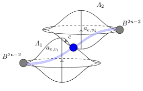
Figure 8. The more accurate front projection of the Legendrian $\varLambda_{1}\cup\varLambda_{2}$ with boundary used to compute $\mathcal{A}_{e}$ for $e\in F_{1}$.

Proof of 1.1.

By 4.2 it suffices to prove that $\mathcal{A}$ is quasi-isomorphic to the relative Ginzburg algebra $\mathscr{G}^{\ast}_{n}(Q,F)$ (see 2.2). Consider the map $\tau\colon\mathcal{A}\to\mathscr{G}^{\ast}_{n}(Q,F)$ defined on generators as

$$\tau(b_{e,v}) =\begin{cases}g_{e}g_{e}^{\ast},&\text{if $e\colon v\to\bullet$}\\ -g_{e}^{\ast}g_{e},&\text{if $e\colon\bullet\to v$}\end{cases},\;\text{$e$ non-frozen},\quad\tau(b_{v})=[g_{e},g_{e}^{\ast}]_{v}^{Q_{1}\smallsetminus F_{1}},\;\text{$v$ frozen}$$

$$\tau(a_{v}) =a_{v},\;\text{$v$ non-frozen},\quad\tau(g_{e})=g_{e},\quad\tau(g_{e}^{\ast})=g_{e}^{\ast},\quad\tau(h_{e})=h_{e}$$

$$\tau(x) =0,\;\text{all other generators},$$

and extended to the whole of $\mathcal{A}$ by linearity and multiplicativity. Furthermore define $\varphi\colon\mathscr{G}^{\ast}_{n}(Q,F)\to\mathcal{A}$ on generators by

$$\varphi(a_{v})=a_{v}-\sum_{e\supset v}a_{e,v},\;\text{$v$ non-frozen},\quad\varphi(x)=x,\;\text{all other generators},$$

and extended to the whole of $\mathscr{G}^{\ast}_{n}(Q,F)$ by linearity and multiplicativity. Finally define $K\colon\mathcal{A}\to\mathcal{\mathcal{missing}}A$ on generators by

$$K(b_{e,v}) =a_{e,v},\quad K(d_{e,v})=\begin{cases}h_{e}c+a^{\prime}_{e,v},&e\colon v\to\bullet\\ -ch_{e}+a^{\prime}_{e,v},&e\colon\bullet\to v\end{cases},\quad K(b_{v})=-a_{v}+\sum_{e\supset v}a_{e,v}$$

$$K(h_{e}^{\ast}) =c,\quad K(x)=0,\;\text{all other generators},$$

and extended to the whole of $\mathcal{A}$ by linearity and as an $(\operatorname{id},\varphi\tau)$-derivation. By an easy but tedious check we have that $\tau$ and $\varphi$ are chain maps and $K$ is a chain homotopy $\varphi\tau\simeq\operatorname{id}$. Applying the gluing formula in 4.2 finishes the first part of the proof.

By [AE22, Remark 2.8] there is a canonical dg-subalgebra $\mathcal{B}\subset CE^{\ast}(\varLambda(Q,F);Z_{0}(Q))$ that is quasi-isomorphic to the dg-subalgebra generated by the boundary $\partial\overline{\varLambda}(Q,F)\subset\partial P_{0}(F)$. By the computation of the dg-algebra $\mathcal{A}$ we have that $\mathcal{B}$ is generated by $\left\{b_{v},d_{e,v},a^{\prime}_{e,v},h_{e},h_{e}^{\ast}\right\}$. By construction the boundary $\partial\overline{\varLambda}(Q,F)\subset\partial P_{0}(F)$ is a smooth Legendrian unknot link so that when attaching a top Weinstein handle to each component of $\partial\overline{\varLambda}(Q,F)$ and call the result $P(F)$, we have that $P(F)$ is a disjoint collection of plumbings of copies of $T^{\ast}S^{n-1}$ according to the quiver $F$. Repeating the above argument with a trivial frozen subquiver with $Q=F$ (or following [Asp23, Section 4.3]) gives the result. To spell it out explicitly, we define maps $\sigma\colon\mathcal{B}\to\mathscr{G}^{\ast}_{n-1}(F)$, $\varepsilon\colon\mathscr{G}^{\ast}_{n-1}(F)\to\mathcal{B}$ and $J\colon\mathcal{B}\to\mathcal{B}$ on generators as

$$\sigma(d_{e,v}) =\begin{cases}h_{e}h_{e}^{\ast},&\text{if $e\colon v\to\bullet$}\\ -h_{e}^{\ast}h_{e},&\text{if $e\colon\bullet\to v$}\end{cases},\quad\sigma(a^{\prime}_{e,v})=0,\quad\sigma(x)=x,\;\text{all other generators}.$$

$$\varepsilon(b_{v}) =b_{v}-\sum_{e\supset v}a^{\prime}_{e,v},\quad\varepsilon(x),\;\text{all other generators}$$

$$J(d_{e,v}) =a^{\prime}_{e,v},\quad J(x)=0\;\text{all other generators}.$$

We extend $\sigma$ and $\varepsilon$ to all of $\mathcal{B}$ and $\mathscr{G}^{\ast}_{n-1}(F)$ by linearity and multiplicativity, and extend $J$ to all of $\mathcal{B}$ by linearity to a $(\operatorname{id},\varepsilon\sigma)$-derivation. As above, an easy check shows that $\sigma$ and $\varepsilon$ are chain maps and $J$ specifies a chain homotopy equivalence $\varepsilon\sigma\simeq\operatorname{id}$. ∎

Proof of 1.3.

This follows from 1.1 together with the easy check that the following diagram commutes.

Here $G$ is the map defined in 2.3. ∎

References

- [AB20] Byung Hee An and Youngjin Bae. A Chekanov–Eliashberg algebra for Legendrian graphs. J. Topol., 13(2):777–869, 2020.
- [AE22] Johan Asplund and Tobias Ekholm. Chekanov–Eliashberg dg-algebras for singular Legendrians. J. Symplectic Geom., 20(3):509–560, 2022.
- [Asp21] Johan Asplund. Fiber Floer cohomology and conormal stops. J. Symplectic Geom., 19(4):777–864, 2021.
- [Asp22] Johan Asplund. Tangle contact homology. arXiv:2210.03036, 2022.
- [Asp23] Johan Asplund. Simplicial descent for Chekanov–Eliashberg dg-algebras. J. Topol., 16(2):489–541, 2023.
- [BC14] Frédéric Bourgeois and Baptiste Chantraine. Bilinearized Legendrian contact homology and the augmentation category. J. Symplectic Geom., 12(3):553–583, 2014.
- [BCS20] Tristan Bozec, Damien Calaque, and Sarah Scherotzke. Relative critical loci and quiver moduli. arXiv:2006.01069, 2020.
- [BD19] Christopher Brav and Tobias Dyckerhoff. Relative Calabi–Yau structures. Compos. Math., 155(2):372–412, 2019.
- [BEE12] Frédéric Bourgeois, Tobias Ekholm, and Yasha Eliashberg. Effect of Legendrian surgery. Geom. Topol., 16(1):301–389, 2012. With an appendix by Sheel Ganatra and Maksim Maydanskiy.
- [Che23] Zhenyi Chen. In preparation, 2023.
- [DRL23] Georgios Dimitroglou Rizell and Noémie Legout. In preparation, 2023.
- [Ekh19] Tobias Ekholm. Holomorphic curves for Legendrian surgery. arXiv:1906.07228, 2019.
- [EL17] Tobias Ekholm and Yankı Lekili. Duality between Lagrangian and Legendrian invariants. arXiv:1701.01284, 2017.
- [EN15] Tobias Ekholm and Lenhard Ng. Legendrian contact homology in the boundary of a subcritical Weinstein 4-manifold. J. Differential Geom., 101(1):67–157, 2015.
- [Gan12] Sheel Ganatra. Symplectic cohomology and duality for the wrapped Fukaya category. ProQuest LLC, Ann Arbor, MI, 2012. Thesis (Ph.D.)–Massachusetts Institute of Technology.
- [Gan19] Sheel Ganatra. Cyclic homology, -equivariant Floer cohomology, and Calabi–Yau structures. arXiv:1912.13510, 2019.
- [GPS18] Sheel Ganatra, John Pardon, and Vivek Shende. Microlocal Morse theory of wrapped Fukaya categories. arXiv:1809.08807, 2018.
- [GPS20] Sheel Ganatra, John Pardon, and Vivek Shende. Covariantly functorial wrapped Floer theory on Liouville sectors. Publ. Math. Inst. Hautes Études Sci., 131:73–200, 2020.
- [Kel11] Bernhard Keller. Deformed Calabi–Yau completions. J. Reine Angew. Math., 654:125–180, 2011. With an appendix by Michel Van den Bergh.
- [KS09] M. Kontsevich and Y. Soibelman. Notes on -algebras, -categories and non-commutative geometry. In Homological mirror symmetry, volume 757 of Lecture Notes in Phys., pages 153–219. Springer, Berlin, 2009.
- [KTV21] Maxim Kontsevich, Alex Takeda, and Yiannis Vlassopoulos. Pre-Calabi–Yau algebras and topological quantum field theories. arXiv:2112.14667, 2021.
- [KW21] Bernhard Keller and Yu Wang. An introduction to relative Calabi–Yau structures. arXiv:2111.10771, 2021.
- [Leg23] Noémie Legout. Calabi–Yau structure on the Chekanov–Eliashberg algebra of a Legendrian sphere. arXiv:2304.03014, 2023.
- [Li19] Yin Li. Koszul duality via suspending Lefschetz fibrations. J. Topol., 12(4):1174–1245, 2019.
- [MS23] Jiajie Ma and Joshua M. Sabloff. In preparation, 2023.
- [Ng23] Lenhard Ng. An structure for Legendrian contact homology. In preparation, 2023.
- [NRS+20] Lenhard Ng, Dan Rutherford, Vivek Shende, Steven Sivek, and Eric Zaslow. Augmentations are sheaves. Geom. Topol., 24(5):2149–2286, 2020.
- [Sei12] Paul Seidel. Fukaya -structures associated to Lefschetz fibrations. I. J. Symplectic Geom., 10(3):325–388, 2012.
- [ST16] Vivek Shende and Alex Takeda. Calabi–Yau structures on topological Fukaya categories. arXiv:1605.02721, 2016.
- [Syl19a] Zachary Sylvan. On partially wrapped Fukaya categories. J. Topol., 12(2):372–441, 2019.
- [Syl19b] Zachary Sylvan. Orlov and Viterbo functors in partially wrapped Fukaya categories. arXiv:1908.02317, 2019.
- [Wu23] Yilin Wu. Relative cluster categories and Higgs categories. Adv. Math., 424:Paper No. 109040, 112, 2023.
- [Yeu16] Wai-Kit Yeung. Relative Calabi–Yau completions. arXiv:1612.06352, 2016.