Neural Structure Learning with Stochastic Differential Equations

Abstract

Discovering the underlying relationships among variables from temporal observations has been a longstanding challenge in numerous scientific disciplines, including biology, finance, and climate science. The dynamics of such systems are often best described using continuous-time stochastic processes. Unfortunately, most existing structure learning approaches assume that the underlying process evolves in discrete-time and/or observations occur at regular time intervals. These mismatched assumptions can often lead to incorrect learned structures and models. In this work, we introduce a novel structure learning method, SCOTCH, which combines neural stochastic differential equations (SDE) with variational inference to infer a posterior distribution over possible structures. This continuous-time approach can naturally handle both learning from and predicting observations at arbitrary time points. Theoretically, we establish sufficient conditions for an SDE and SCOTCH to be structurally identifiable, and prove its consistency under infinite data limits. Empirically, we demonstrate that our approach leads to improved structure learning performance on both synthetic and real-world datasets compared to relevant baselines under regular and irregular sampling intervals.

1 Introduction

Time-series data are ubiquitous in the real world, often comprising a series of data points recorded at varying time intervals. Understanding the underlying structures between variables associated with temporal processes is of paramount importance for numerous real-world applications (Spirtes et al.,, 2000; Berzuini et al.,, 2012; Peters et al.,, 2017). Although randomised experiments are considered the gold standard for unveiling such relationships, they are frequently hindered by factors such as cost and ethical concerns. Structure learning seeks to infer hidden structures from purely observational data, offering a powerful approach for a wide array of applications (Bellot et al.,, 2021; Löwe et al.,, 2022; Runge,, 2018; Tank et al.,, 2021; Pamfil et al.,, 2020; Gong et al.,, 2022).

However, many existing structure learning methods for time series are inherently discrete, assuming that the underlying temporal processes are discretized in time and requiring uniform sampling intervals throughout the entire time range. Consequently, these models face two key limitations: (i) they may misrepresent the true underlying process when it is continuous in time, potentially leading to incorrect inferred relationships; and (ii) they struggle with handling irregular sampling intervals, which frequently arise in fields such as biology (Trapnell et al.,, 2014; Qiu et al.,, 2017; Qian et al.,, 2020) and climate science (Bracco et al.,, 2018; Raia,, 2008). Although there exists a previous work (Bellot et al.,, 2021) that also tries to infer the underlying structure from the continuous-time perspective, its framework based on ordinary differential equations (ODE) is intrinsically flawed, and we show that it cannot correctly learn the underlying system under multiple time series settings.

To address these challenges, we introduce a novel structure learning framework, Structure learning with COntinuous-Time stoCHastic models (SCOTCH), which combines stochastic differential equations (SDEs) and variational inference (VI) to model the underlying temporal processes. Owing to its continuous nature, SCOTCH can manage irregularly sampled time series and accurately represent continuous processes. We make the following key contributions:

1. We introduce a novel latent Stochastic Differential Equation (SDE) formulation for modelling continuous-time observational time-series data. To effectively train our proposed model, which we denote as SCOTCH, we adapt the variational inference framework proposed in (Li et al.,, 2020; Tzen and Raginsky, 2019a, ) to approximate the posterior for both the underlying graph structure and the latent variables. In contrast to the previous ODE-based approach, our model is capable of accurately learning the underlying dynamics.

2. We provide a rigorous theoretical analysis to support our proposed methodology. Specifically, we prove that when SDEs are directly employed for modelling the observational process, the resulting SDEs are structurally identifiable under global Lipschitz and diagonal noise assumptions. We also prove our model maintains structural identifiability under certain conditions, even when adopting the latent formulation and that variational inference, when integrated with the latent formulation, in the infinite data limit, can successfully recover the ground truth graph structure and mechanisms under specific assumptions.

3. Empirically, we derive a failure case where the previous approach failed to learn the ground truth compared to ours. Additionally, we conduct extensive experiments on both synthetic and real-world datasets that SCOTCH can improve upon existing methods on structure learning, including when the data is irregularly sampled.

2 Preliminaries

Notations

We use ${\bm{X}}_{t}\in\mathbb{R}^{D}$ to denote the $D$-dimensional observation vector at time $t$, with $X_{t,d}$ representing the $d^{\text{th}}$ variable of the observation. A time series is a set of $I$ observations ${\bm{X}}=\{{\bm{X}}_{t_{i}}\}_{t=1}^{I}$, where $\{t_{i}\}_{i=1}^{I}$ are the observation times. In the case where we have multiple ($N$) i.i.d. time series, we use ${\bm{X}}^{(n)}$ to indicate the $n^{\text{th}}$ time series.

Bayesian structure learning

In structure learning, the aim is to infer the graph representing the relationships between variables from data. Given time series data $\{{\bm{X}}^{(n)}\}_{n=1}^{N}$, the joint distribution over graphs and data is given by:

$$p_{\theta}({\bm{G}},{\bm{X}}^{(1)},\ldots,{\bm{X}}^{(N)})=p({\bm{G}})\prod_{n=1}^{N}p_{\theta}({\bm{X}}^{(n)}|{\bm{G}})$$ (1)

where $p({\bm{G}})$ is the graph prior and $p({\bm{X}}^{(n)}|{\bm{G}})$ is the likelihood term. The goal is then to compute the graph posterior $p({\bm{G}}|{\bm{X}})$. However, analytic computation is intractable for high dimensional settings. Therefore, variational inference (Zhang et al.,, 2018) and sampling methods (Welling and Teh,, 2011; Gong et al.,, 2018; Annadani et al.,, 2023) are commonly used for inference.

Structural equation models (SEMs)

Given a time series ${\bm{X}}$ and graph ${\bm{G}}\in\{0,1\}^{D\times D}$, we can use SEMs to describe the structural relationships between variables:

$$X_{t,d}=f_{t,d}({\bm{Pa}_{\bm{G}}}^{d}(<t),\epsilon_{t,d})$$ (2)

where ${\bm{Pa}_{\bm{G}}}^{d}(<t)$ specifies the lagged parents of $X_{t,d}$ at previous time and $\epsilon_{t,d}$ is the mutually independent noise. Such a model requires discrete time steps that are usually assumed to follow a regular sampling interval, i.e. $t_{i+1}-t_{i}$ is a constant for all $i=1,\ldots,I-1$. Most existing models can be regarded as a special case of this framework.

Itô diffusion

A time-homogenous Itô diffusion is a stochastic process ${\bm{X}}_{t}$ and has the form:

$$d{\bm{X}}_{t}={\bm{f}}({\bm{X}}_{t})dt+{\bm{g}}({\bm{X}}_{t})d{\bm{W}}_{t}$$ (3)

where ${\bm{f}}:\mathbb{R}^{D}\rightarrow\mathbb{R}^{D},{\bm{g}}:\mathbb{R}^{D}\rightarrow\mathbb{R}^{D\times D}$ are time-homogeneous drift and diffusion functions, respectively, and ${\bm{W}}_{t}$ is a Brownian motion under the measure $P$. It is known that under global Lipschitz guarantees (Assumption 1) it has a unique strong solution (Øksendal and Øksendal,, 2003).

Euler discretization and Euler SEM

For most Itô diffusions, the analytic solution ${\bm{X}}_{t}$ is intractable, especially with non-linear drift and diffusion functions. Thus, we often seek to simulate the trajectory by discretization. One common scheme is called Euler-Maruyama (EM) scheme. With a fixed step size $\Delta$, EM simulates the trajectory as

$${\bm{X}^{\Delta}_{t+1}}={\bm{X}^{\Delta}_{t}}+{\bm{f}}({\bm{X}^{\Delta}_{t}})\Delta+{\bm{g}}({\bm{X}^{\Delta}_{t}})\eta_{t}$$ (4)

where ${\bm{X}^{\Delta}_{t}}$ is the random variable induced by discretization and $\eta_{t}\sim\mathcal{N}(0,\Delta)$. Notice that eq. 4 is a special case of eq. 2. If we define the graph ${\bm{G}}$ as the following: if ${\bm{X}}^{\Delta}_{t,i}\rightarrow{\bm{X}}^{\Delta}_{t+1,j}$ in ${\bm{G}}$, then $\frac{\partial f_{j}({\bm{X}^{\Delta}_{t}})}{\partial X^{\Delta}_{t,i}}\neq 0$ or $\exists k,\frac{\partial g_{j,k}({\bm{X}^{\Delta}_{t}})}{\partial X^{\Delta}_{t,i}}\neq 0$; and assume ${\bm{g}_{G}}$ only outputs a diagonal matrix, then the above EM induces a temporal SEM, called Euler SEM (Hansen and Sokol,, 2014), which provides a useful analysis tool for continuous time processes.

3 SCOTCH: Bayesian Structure Learning for Continuous Time Series

We consider a dynamical system in which there is both intrinsic stochasticity in the evolution of the state, as well as independent measurement noise that is present in the observed data. For example, in healthcare, the condition of a patient will progress with randomness rather than deterministically. On the other hand, the measurement of patient status will also be affected by the accuracy of the equipment, where the noise is independent to the intrinsic stochasticity. To account for the above behaviour, we propose to use the latent SDE formulation (Li et al.,, 2020; Tzen and Raginsky, 2019a, ):

$$d{\bm{Z}}_{t} ={\bm{f}}_{\theta}({\bm{Z}}_{t})dt+{\bm{g}}_{\theta}({\bm{Z}}_{t})d{\bm{W}}_{t}\text{ (latent process)}$$

$${\bm{X}}_{t} ={\bm{Z}}_{t}+\bm{\epsilon}_{t}\text{ (noisy observations)}$$ (5)

where ${\bm{Z}}_{t}\in\mathbb{R}^{D}$ is the latent variable representing the internal state of the dynamic system, ${\bm{X}}_{t}\in\mathbb{R}^{D}$ describes the observational data with the same dimension, $\bm{\epsilon_{t}}$ is additive Gaussian noise with diagonal covariance matrix, ${\bm{f}}_{\theta}:\mathbb{R}^{D}\rightarrow\mathbb{R}^{D}$ is the drift function, ${\bm{g}}_{\theta}:\mathbb{R}^{D}\rightarrow\mathbb{R}^{D}$ is the diffusion function and ${\bm{W}}_{t}$ is the Wiener process. A key distinction of our model from the general Itô diffusion (eq. 3) is its use of a nonzero diagonal diffusion function (Assumption 2 in section A.1), ${\bm{g}}_{\theta}$, rather than a full diffusion matrix, enabling structural identifiability as we show in the next section.

Signature graph

In accordance with the graph defined in Euler SEMs (section 2), we define the graph ${\bm{G}}$ as follows: edge $i\rightarrow j$ is present in ${\bm{G}}$ iff  $\exists t$ s.t. either $\frac{\partial f_{j}({\bm{Z}}_{t})}{\partial Z_{t,i}}\neq 0$ or $\frac{\partial g_{j}({\bm{Z}}_{t})}{\partial Z_{t,i}}\neq 0$. Note that there is no requirement for the graph to be acyclic. Intuitively, the graph ${\bm{G}}$ describes the structural dependence between variables.

To present SCOTCH, we first define the prior and likelihood components:

Prior over Graphs

Leveraging Geffner et al., (2022); Annadani et al., (2023), our graph prior is designed as:

$$p({\bm{G}})\propto\exp(-\lambda_{s}\|{\bm{G}}\|_{F}^{2})$$ (6)

where $\lambda_{s}$ is the graph sparsity coefficient, and $\|\cdot\|_{F}$ is the Frobenious norm.

Prior process

Since the latent process induces a distribution over latent trajectories before seeing any observations, we also call it the prior process. We propose to use neural networks for drift and diffusion functions ${\bm{f}}_{\theta}:\mathbb{R}^{D}\times\{0,1\}^{D\times D}\rightarrow\mathbb{R}^{D}$, ${\bm{g}}_{\theta}:\mathbb{R}^{D}\times\{0,1\}^{D\times D}\rightarrow\mathbb{R}^{D}$, which explicitly take the latent state and the graph as inputs. Note that although the signature graph is defined through the function derivatives, we explicitly use the graph ${\bm{G}}$ as input to denote their dependence. We will interchangeably use the notation ${\bm{f}_{G}}$ and ${\bm{g}_{G}}$ to denote ${\bm{f}}_{\theta}(\cdot,{\bm{G}})$ and ${\bm{g}}_{\theta}(\cdot,{\bm{G}})$. To design the graph-dependent drift and diffusion, we leverage the design of Geffner et al., (2022) and propose:

$${\bm{f}}_{G,d}({\bm{Z}}_{t})=\zeta\left(\sum_{i=1}^{D}G_{i,d}l(Z_{t,i},{\bm{e}}_{i}),{\bm{e}}_{d}\right)$$ (7)

for both ${\bm{f}_{G}}$ and ${\bm{g}_{G}}$, where $\zeta$, $l$ are neural networks, and ${\bm{e}}_{i}$ is a trainable node embedding for the $i^{\text{th}}$ node. The corresponding prior process is:

$$d{\bm{Z}}_{t} ={\bm{f}}_{\theta}({\bm{Z}}_{t},{\bm{G}})dt+{\bm{g}}_{\theta}({\bm{Z}}_{t},{\bm{G}})d{\bm{W}}_{t}\text{ (prior process)}$$ (8)

Likelihood of time series

Given a time series $\{{\bm{X}}_{t_{i}}\}_{i=1}^{I}$, the likelihood is defined as

$$p(\{{\bm{X}}_{t_{i}}\}_{i=1}^{I}|\{{\bm{Z}}_{t_{i}}\}_{i=1}^{I},{\bm{G}})=\prod_{i=1}^{I}\prod_{d=1}^{D}\mathcal{N}(Z_{t_{i},d},\sigma_{t_{i},d}^{2})$$ (9)

where $\sigma_{t_{i},d}^{2}$ is the variance of noise $\epsilon_{t_{i},d}$.

3.1 Variational Inference

Suppose that we are given multiple time series $\{{\bm{X}}^{(n)}\}_{n=1}^{N}$ as observed data from the system. The goal is then to compute the posterior over graph structures $p({\bm{G}}|\{{\bm{X}}^{(n)}\}_{n=1}^{N})$, which is intractable. Thus, we leverage variational inference to simultaneously approximate both the graph posterior, and a latent posterior process over ${\bm{Z}}^{(n)}$ for every observed time series ${\bm{X}}^{(n)}$. Given $N$ i.i.d time series $\{{\bm{X}}^{(n)}\}_{n=1}^{N}$, we propose to use a variational approximation $q_{\phi}({\bm{G}})\approx p({\bm{G}}|{\bm{X}}^{(1)},\ldots,{\bm{X}}^{(N)})$. With the standard trick from variational inference, we have the following evidence lower bound (ELBO):

$$\log p({\bm{X}}^{(1)},\ldots,{\bm{X}}^{(N)})\geq\mathbb{E}_{q_{\phi}({\bm{G}})}\left[\sum_{n=1}^{N}\log p_{\theta}({\bm{X}}^{(n)}|{\bm{G}})\right]-D_{\mathrm{KL}}(q_{\phi}({\bm{G}})\|p({\bm{G}}))$$ (10)

Unfortunately, the distribution $p_{\theta}({\bm{X}}^{(n)}|{\bm{G}})$ remains intractable due to the marginalization of the latent Itô diffusion ${\bm{Z}}^{(n)}$. Therefore, we leverage the variational framework proposed in Tzen and Raginsky, 2019a ; Li et al., (2020) to approximate the true posterior $p({\bm{Z}}^{(n)}|{\bm{X}}^{(n)},{\bm{G}})$. For each $n=1,\ldots,N$, the variational posterior $q_{\psi}(\tilde{{\bm{Z}}}^{(n)}|{\bm{X}}^{(n)},{\bm{G}})$ is given by the solution to the following:

$${\tilde{\bm{Z}}}_{t,0}^{(n)}\sim\mathcal{N}({\bm{\mu}}_{\psi}({\bm{G}},{\bm{X}}^{(n)}),{\bm{\Sigma}}_{\psi}({\bm{G}},{\bm{X}}^{(n)}))\;\;\;\text{(posterior initial state)}$$

$$d{\tilde{\bm{Z}}}_{t}^{(n)}={\bm{h}}_{\psi}({\tilde{\bm{Z}}}_{t}^{(n)},t;{\bm{G}},{\bm{X}}^{(n)})dt+{\bm{g}_{G}}({\tilde{\bm{Z}}}_{t}^{(n)})d{\bm{W}}_{t}\;\;\;\text{(posterior process)}$$ (11)

For the initial latent state, ${\bm{\mu}}_{\psi},{\bm{\Sigma}}_{\psi}$ are posterior mean and covariance functions implemented as neural networks. For the SDE, we use the same diffusion function ${\bm{g}_{G}}$ for both the prior and posterior processes, but train a separate neural drift function ${\bm{h}}_{\psi}$ for the posterior, which takes a time series ${\bm{X}}^{(n)}$ as input. The posterior drift function differs from the prior in two key ways. Firstly, the posterior drift function depends on time; this is necessary as conditioning on the observed data creates this dependence even when the prior process is time-homogenous. Secondly, while ${\bm{h}}_{\psi}$ takes the graph ${\bm{G}}$ as an input, the function design is not constrained to have a matching signature graph like ${\bm{f}_{G}}$. More details on the implementation of ${\bm{h}}_{\psi},{\bm{\mu}}_{\psi},{\bm{\Sigma}}_{\psi}$ can be found in Appendix B.

Assume for each time series ${\bm{X}}^{(n)}$, we have observation times $t_{i}$ for $i=1,\ldots,I$ within the time range $[0,T]$, then, we have the following evidence lower bound for $\log p({\bm{X}}^{(n)}|{\bm{G}})$ (Li et al.,, 2020):

$$\log p({\bm{X}}^{(n)}|{\bm{G}})\geq\mathbb{E}_{q_{\psi}}\left[\sum_{i=1}^{I}\log p({\bm{X}}^{(n)}_{t_{i}}|{\tilde{\bm{Z}}}^{(n)}_{t_{i}},{\bm{G}})-\int_{0}^{T}\|{\bm{u}}^{(n)}({\tilde{\bm{Z}}}^{(n)}_{t})\|^{2}dt\right]$$ (12)

where ${\tilde{\bm{Z}}}^{(n)}_{t}$ is the posterior process modelled by eq. 11 and ${\bm{u}}^{(n)}({\tilde{\bm{Z}}}^{(n)}_{t})$ is given by:

$${\bm{u}}^{(n)}({\tilde{\bm{Z}}}^{(n)}_{t})={\bm{g}_{G}}({\tilde{\bm{Z}}}_{t}^{(n)})^{-1}({\bm{h}}_{\psi}({\tilde{\bm{Z}}}_{t}^{(n)},t;{\bm{G}},{\bm{X}}^{(n)})-{\bm{f}}_{G}({\tilde{\bm{Z}}}_{t}^{(n)}))$$ (13)

By combining eq. 10 and eq. 12, we derive an overall ELBO:

$$\log p_{\theta}({\bm{X}}^{(1)},\ldots,{\bm{X}}^{(N)})\geq \mathbb{E}_{q_{\phi}}\left[\sum_{n=1}^{N}\mathbb{E}_{q_{\psi}}\left[\sum_{i=1}^{I}\log p({\bm{X}}_{t_{i}}^{(n)}|{\tilde{\bm{Z}}}_{t_{i}}^{(n)},{\bm{G}})-\int_{0}^{T}\|{\bm{u}}^{(n)}({\tilde{\bm{Z}}}_{t}^{(n)})\|^{2}dt\right]\right]$$

$$-D_{\mathrm{KL}}(q_{\phi}({\bm{G}})\|p({\bm{G}}))$$ (14)

In practice, we approximate the ELBO (and its gradients) using a Monte-Carlo approximation. The inner expectation can be approximated by simulating from an augmented version of eq. 11 where an extra variable $L$ is added with drift $\frac{1}{2}|{\bm{u}}^{(n)}({\tilde{\bm{Z}}}^{(n)}_{t})|^{2}$ and diffusion zero (Li et al.,, 2020). Algorithm 1 summarizes the training algorithm of SCOTCH.

Algorithm 1 SCOTCH training

  Input: i.i.d time series $\{{\bm{X}}^{(n)}\}_{n=1}^{N}$; drift functions ${\bm{f}_{G}}$, ${\bm{h}}_{\psi}$, diffusion function ${\bm{g}_{G}}$, SDE solver $\operatorname*{Solver}$, initial condition ${\tilde{\bm{Z}}}_{0}^{(n)}$, training iterations L

  for $l=1,\ldots,L$ do

     Sample time series mini-batch $\{{\bm{X}}^{(n)}\}_{n=1}^{S}$ with batch size $S$.

     for $n=1,\ldots,S$ do

        Draw graph ${\bm{G}}\sim q_{\phi}({\bm{G}})$

        Draw initial latent state $\tilde{{\bm{Z}}}^{(n)}_{0}\sim\mathcal{N}({\bm{\mu}}_{\psi}({\bm{G}},{\bm{X}}^{(n)}),{\bm{\Sigma}}_{\psi}({\bm{G}},{\bm{X}}^{(n)}))$

        Solve (sample from) the posterior process $({\tilde{\bm{Z}}}^{(n)},L)=\operatorname*{Solver}(({\tilde{\bm{Z}}}^{(n)}_{0},0),{\bm{f}_{G}},{\bm{h}}_{\psi},{\bm{g}_{G}})$

     end for

     Maximize ELBO eq. 14 w.r.t. $\phi,\psi,\theta$

  end for

3.2 Comparison to Related Work

NGM

Bellot et al., (2021) proposed a structure learning method, called NGM, to learn from single time series generated by SDEs. NGM uses a neural ODE to model the mean process ${\bm{f}}_{\theta}$, and extracts graphical structure from the first layer of ${\bm{f}}_{\theta}$. However, NGM assumes that the observed single series ${\bm{X}}$ follows a multivariate Gaussian distribution, which only holds for linear SDEs. If this assumption is violated, optimizing their proposed squared loss cannot recover the underlying system. SCOTCH does not have this limitation and can handle more flexible state-dependent drifts and diffusions. Another drawback of NGM is its inability to handle multiple time series ($N>1$). Learning from multiple series is important when dealing with SDEs with multimodal behaviour. We propose a simple bimodal 1-D failure case: $dX=Xdt+0.01dW_{t},X_{0}=0$, with the signature graph containing a self-loop. Figure 1 shows the bimodal trajectories (upwards and downwards) sampled from the SDE. The optimal ODE mean process in this case is the constant ${\bm{f}}_{\theta}=0$ with an empty graph, as confirmed by the learned mean process of NGM (black line in fig. 1(b)). In contrast, SCOTCH can learn the underlying SDE and simulate the correct trajectories (fig. 1(c)).

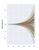
(a) Data

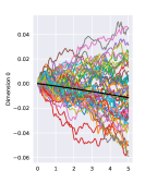
(b) NGM

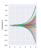
(c) SCOTCH

Figure 1: Comparison between NGM and SCOTCH for simple SDE (note vertical axis scale)

Rhino

Gong et al., (2022) proposed a flexible discretised temporal SEM that is capable of modelling (1) lagged parents; (2) instantaneous effect; and (3) history dependent noise. Rhino’s SEM is given by $X_{t,d}=f_{d}({\bm{Pa}_{\bm{G}}}^{d}(<t),{\bm{Pa}_{\bm{G}}}^{d}(t))+g_{d}({\bm{Pa}_{\bm{G}}}^{d}(<t))\epsilon_{t,d}$. We can clearly see its similarity to SCOTCH. If $f_{d}$ has a residual structure as $f_{d}(\cdot)=X_{t,d}+r_{d}(\cdot)\Delta$ and we assume no instantaneous effect (${\bm{Pa}_{\bm{G}}}^{d}(t)$ is empty), Rhino SEM is equivalent to the Euler SEM of the latent process (eq. 8) with drift ${\bm{r}}$, step size $\Delta$ and diagonal diffusion ${\bm{g}}$. Thus, similar to the relation of ResNet (He et al.,, 2016) to NeuralODE (Chen et al.,, 2018), SCOTCH is the continuous-time analog of Rhino.

3.3 Intervention

Aside from learning the graphical structure between variables, one might also be interested in predicting the effect of applying external changes, or interventions, to the system. Broadly speaking, there are two types of interventions that we can consider in a continuous-time model. The first is to intervene on the dynamics (i.e. the drift or diffusion functions), possibly for a set period of time. The second is to directly intervene on the value of (some subset of) variables. Our model can handle both types of interventions by modifying how we simulate the latent SDE to predict the corresponding effects. For more details, see appendix E.

4 Theoretical considerations of SCOTCH

In this section, we aim to answer three important theoretical questions regarding the Itô diffusion proposed in section 3. For notational simplicity, we consider the single time series setting. First, we examine when a general Itô diffusion is structurally identifiable. Secondly, we consider structural identifiability in the latent formulation of eq. 5. Finally, we consider whether optimising ELBO (eq. 14) can recover the true graph and mechanism if we have infinite observations for a single time series within a fixed time range $[0,T]$. All detailed proofs, definitions, and assumptions can be found in appendix A.

4.1 Structure identifiability

Suppose that the observational process is given as an Itô diffusion:

$$d{\bm{X}}_{t}={\bm{f}_{G}}({\bm{X}}_{t})dt+{\bm{g}_{G}}({\bm{X}}_{t})d{\bm{W}}_{t}$$ (15)

Then we might ask what are sufficient conditions for the model to be structurally identifiable? That is, there does not exist ${\bm{G}}^{\prime}\neq{\bm{G}}$ that can induce the same observational distribution.

Theorem 4.1 (Structure identifiability of the observational process).

Given eq. 15, let us define another process with $\bar{{\bm{X}}}_{t}$, ${\bm{G}}\neq\bar{{\bm{G}}}$, ${\bm{\bar{f}}_{\bar{G}}}$, ${\bm{\bar{g}}_{\bar{G}}}$ and $\bar{{\bm{W}}}_{t}$. Then, under Assumptions 1-2, and with the same initial condition ${\bm{X}}(0)={\bm{\bar{X}}}(0)={\bm{x}}_{0}$, the solutions ${\bm{X}}_{t}$ and ${\bm{\bar{X}}}_{t}$ will have different distributions.

Next, we show that structural identifiability is preserved, under certain conditions, even in the latent formulation where the SDE solution is not directly observed.

Theorem 4.2 (Structural identifiability with latent formulation).

Consider the distributions $p,{\bar{p}}$ defined by the latent model in eq. 5 with $({\bm{G}},{\bm{Z}},{\bm{X}},{\bm{f}_{G}},{\bm{g}_{G}}),({\bar{\bm{G}}},{\bar{\bm{Z}}},{\bm{\bar{X}}},{\bm{\bar{f}}_{\bar{G}}},{\bm{\bar{g}}_{\bar{G}}})$ respectively, where ${\bm{G}}\neq{\bar{\bm{G}}}$. Further, let $t_{1},\ldots,t_{I}$ be the observation times. Then, under Assumptions 1 and 2:

1. if $t_{i+1}-t_{i}=\Delta$ for all $i\in 1,...,I-1$, then $p^{\Delta}({\bm{X}}_{t_{1}},\ldots,{\bm{X}}_{t_{I}})\neq{\bar{p}}^{\Delta}({\bm{\bar{X}}}_{t_{1}},\ldots,{\bm{\bar{X}}}_{t_{I}})$, where $p^{\Delta}$ is the density generated by the Euler discretized eq. 8 for ${\bm{Z}}_{t}$;

2. if we have a fixed time range $[0,T]$, then the path probability $p({\bm{X}}_{t_{1}},\ldots,{\bm{X}}_{t_{I}})\neq{\bar{p}}({\bm{\bar{X}}}_{t_{1}},\ldots,{\bm{\bar{X}}}_{t_{I}})$ under the limit of infinite data ($I\rightarrow\infty$).

4.2 Consistency

Building upon the structural identifiability, we can prove the consistency of the variational formulation. Namely, in the infinite data limit, one can recover the ground truth graph and mechanism by maximizing ELBO with a sufficiently expressive posterior process and a correctly specified model.

Theorem 4.3 (Consistency of variational formulation).

Suppose Assumptions 1-25 are satisfied for the latent formulation (eq. 5). Then, for a fixed observation time range $[0,T]$, as the number of observations $I\rightarrow\infty$, when ELBO (eq. 14) is maximised, $q_{\phi}({\bm{G}})=\delta({\bm{G}}^{*})$, where ${\bm{G}}^{*}$ is the ground truth graph, and the latent formulation recovers the underlying ground truth mechanism.

Expressiveness of the posterior process

One central assumption is that the posterior process should be expressive enough to approximate the actual posterior over ${\bm{Z}}_{t}$. Since we use neural networks to define the drift and diffusion functions, the corresponding approximate posterior is flexible. In fact, Tzen and Raginsky, 2019b showed that the diffusion defined by eq. 11 can be used to obtain samples from any distributions whose Radon-Nikodym derivative w.r.t. standard Gaussian measure can be represented by neural networks. Due to the universal approximation of neural network (Hornik et al.,, 1989), the corresponding posterior is indeed flexible.

5 Related work

Discrete time causal models

The majority of the existing approaches are inherently discrete in time. Assaad et al., (2022) provides a comprehensive overview. There are three types of discovery methods: (1) Granger causality; (2) structure equation model (SEM); and (3) constraint-based methods. Granger causality assumes that no instantaneous effects are present and the causal direction cannot flow backward in time. Wu et al., (2020); Shojaie and Michailidis, (2010); Siggiridou and Kugiumtzis, (2015); Amornbunchornvej et al., (2019) leverage the vector-autoregressive model to predict future observations. Löwe et al., (2022); Tank et al., (2021); Bussmann et al., (2021); Dang et al., (2019); Xu et al., (2019); Khanna and Tan, (2019) utilise deep neural networks for prediction. Recently, Cheng et al., (2023) introduced a deep-learning based Granger causality that can handle irregularly sampled data, treating it as a missing data problem and proposing a joint framework for data imputation and graph fitting. SEM based approaches assume an explicit causal model associated to the temporal process. Hyvärinen et al., (2010) leverages the identifiability of additive noise models (Hoyer et al.,, 2008) to build a linear auto-regressive SEM with non-Gaussian noise. Pamfil et al., (2020) utilises the NOTEARS framework (Zheng et al.,, 2018) to continuously relax the DAG constraints for fully differentiable structure learning. The recently proposed Gong et al., (2022) extended the prior DECI Geffner et al., (2022) framework to handle time series data and is capable of modelling instantaneous effect and history-dependent noise. Constraint-based approaches use conditional independence tests to determine the causal structures. Runge et al., (2019) combines the PC (Spirtes et al.,, 2000) and momentary conditional independence tests for the lagged parents. PCMCI+ (Runge,, 2020) can additionally detect the instantaneous effect. LPCMCI (Reiser,, 2022) can further handle latent confounders. CD-NOD (Zhang et al.,, 2017) is designed to handle non-stationary heterogeneous time series data. However, all constraint-based approaches can only identify the graph up to Markov equivalence class without the functional relationship between variables.

Continuous time causal models

In terms of using differential equations to model the continuous temporal process, Hansen and Sokol, (2014) proposed using stochastic differential equations to describe the temporal causal system. They proved identifiability with respect to the intervention distributions, but did not show how to learn a corresponding SDE. Penalised regression has been explored for linear models, where parameter consistency has been established (Ramsay et al.,, 2007; Chen et al.,, 2017; Wu et al.,, 2014). Recently, NGM (Bellot et al.,, 2021) uses ODEs to model the temporal process with both identifiability and consistency results. As discussed in previous sections, SCOTCH is based on SDEs rather than ODEs, and can model the intrinsic stochasticity within the causal system, whereas NGM assumes deterministic state transitions.

6 Experiments

Baselines and Metrics

We benchmark our method against a representative sample of baselines: (i) VARLiNGaM (Hyvärinen et al.,, 2010), a linear SEM based approach; (ii) PCMCI+ (Runge,, 2018, 2020), a constraint-based method for time series; (iii) CUTS, a Granger causality approach which can handle irregular time series; (iv) Rhino (Gong et al.,, 2022), a non-linear SEM based approach with history-dependent noise and instantaneous effects; and (v) NGM (Bellot et al.,, 2021), a continuous-time ODE based structure learner. Since most methods require a threshold to determine the graph, we use the threshold-free area under the ROC curve (AUROC) as the performance metric. In appendix D, we also report F1 score, true positive rate (TPR) and false discovery rate (FDR).

Setup

Both the synthetic datasets (Lorenz-96, Glycolysis) and real-world datasets (DREAM3, Netsim) consist of multiple time series. However, it is not trivial to modify NGM and CUTS to support multiple time series. For fair comparison, we use the concatenation of multiple time series, which we found empirically to improve performance. We also mimic irregularly sampled data by randomly dropping observations, which VARLiNGaM, PCMCI, and Rhino cannot handle; in these cases, for these methods we impute the missing data using zero-order hold (ZOH). Further details can be found in Appendices B, C, D.

6.1 Synthetic experiments: Lorenz and Glycolysis

First, we evaluate SCOTCH on synthetic benchmarks including the Lorenz-96 (Lorenz,, 1996) and Glycolysis (Daniels and Nemenman,, 2015) datasets, which model continuous-time dynamical systems. The Lorenz model is a well-known example of chaotic systems observed in biology (Goldberger and West,, 1987; Heltberg et al.,, 2019).To mimic the irregular sampled data, we follow the setup of Cheng et al., (2023) and randomly drop some observations with missing probability $p$. To verify the advantages of using SDE models, we also simulate another dataset from a biological model, which describes metabolic iterations that break down glucose in cells. This is called Glycolysis, consisting of an SDE with $7$ variables. As a preprocessing step, we standardised this dataset to avoid large differences in variable scales. Both datasets consist of $N=10$ time series with sequence length $I=100$ (before random drops), and have dimensionality $10$ and $7$, respectively. Note that we choose a large data sampling interval, as we want to test settings where observations are fairly sparse and the difficulty of correctly modelling continuous-time dynamics increases. The above data setup is different from Bellot et al., (2021); Cheng et al., (2023) where they use a single series with $I=1000$ observations, which is more informative compared to our sparse setting. Refer to section D.1 and section D.2 for details.

Lorenz results

The left two columns in table 1 compare the AUROC of SCOTCH to baselines. We can see that SCOTCH can effectively handle the irregularly sampled data compared to other baselines. Compared to NGM and CUTS, we can achieve much better results with small missingness and performs competitively with larger missingness. Rhino, VARLiNGaM and PCMCI+ perform poorly in comparison as they assume regularly sampled observations and are discrete in nature.

Glycolysis results

From the right column in table 1, SCOTCH outperform the baselines by a large margin. In particular, compared to the ODE-based NGM, SCOTCH clearly demonstrate the advantage of the proposed SDE framework in multiple time series settings. As we may have anticipated from the discussion in section 3.2, NGM can produce an incorrect model when multiple time series are sampled from a given SDE system. Another interesting observation is that SCOTCH is more robust when encountering data with different scales compared to NGM (refer to section D.2.3). This robustness is due to the stochastic nature of SDE compared to the deterministic ODE, where ODE can easily overshoot with less stable training behaviour. We can also see that SCOTCH has a significant advantage over both CUTS and Rhino, which do not model continuous-time dynamics.

	Lorenz-96		Glycolysis
	$p=0.3$	$p=0.6$	Full
VARLiNGaM	0.5102$\pm$0.025	0.4876$\pm$0.032	0.5082$\pm$0.009
PCMCI+	0.4990$\pm$0.008	0.4952$\pm$0.021	0.4607$\pm$0.031
NGM	0.6788$\pm$0.009	0.6329$\pm$0.008	0.5953$\pm$0.018
CUTS	0.6042$\pm$0.015	0.6418$\pm$0.012	0.580$\pm$0.007
Rhino	0.5714$\pm$0.026	0.5123$\pm$0.025	0.520$\pm$0.015
SCOTCH (ours)	0.7279$\pm$0.017	0.6453$\pm$0.014	0.7113$\pm$0.012

Table 1: AUROC of synthetic datasets from SCOTCH and baselines. $p$ represents missing probability, and Full means complete data without missingness. Each number is the average over $5$ runs.

6.2 Dream3

We also evaluate SCOTCH performance on the DREAM3 datasets (Prill et al.,, 2010; Marbach et al.,, 2009), which have been adopted for assessing the performance of structure learning (Tank et al.,, 2021; Pamfil et al.,, 2020; Gong et al.,, 2022). These datasets contain in silico measurement of gene expression levels for $5$ different structures. Each dataset corresponds to a particular gene expression network, and contains $N=46$ time series of 100 dimensional variables, with $I=21$ per series. The goal is to infer the underlying structures from each dataset. Following the same setup as (Gong et al.,, 2022; Khanna and Tan,, 2019), we ignore all the self-connections by setting the edge probability to $0$, and use AUROC as the performance metric. Section D.3 details the experiment setup, selected hyperparameters, and additional plots. We do not include VARLiNGaM since it cannot support the series where the dimensionality ($100$) is greater than the length ($21$). Also due to the time series length, we decide not to test with irregularly sampled data. For CUTS, we failed to reproduce the reported number in their paper, but we cite it for a fair comparison.

Table 2 shows the AUROC performances of SCOTCH and baselines. We can clearly observe that SCOTCH outperforms the other baselines with a large margin. This indicates the advantage of the SDE formulation compared to ODEs and discretized temporal models, even when we have complete and regularly sampled data. A more interesting observation is to compare Rhino with SCOTCH. As discussed before, as SCOTCH is the continuous version of Rhino, the advantage comes from the continuous formulation and the corresponding training objective eq. 14.

	EColi1	Ecoli2	Yeast1	Yeast2	Yeast3	Mean
PCMCI+	0.530$\pm$0.002	0.519$\pm$0.002	0.530 $\pm$0.003	0.510$\pm$0.001	0.512 $\pm$ 0	0.520$\pm$0.004
NGM	0.611$\pm$0.002	0.595$\pm$0.005	0.597$\pm$0.006	0.563$\pm$0.006	0.535$\pm$0.004	0.580$\pm$0.007
CUTS	0.543$\pm$0.003	0.555$\pm$0.005	0.545$\pm$0.003	0.518$\pm$0.007	0.511$\pm$0.002	0.534$\pm$0.008 (0.591)
Rhino	0.685$\pm$0.003	0.680$\pm$0.007	0.664$\pm$0.006	0.585$\pm$0.004	0.567$\pm$0.003	0.636$\pm$0.022
SCOTCH (ours)	0.752$\pm$0.008	0.705$\pm$0.003	0.712$\pm$0.003	0.622 $\pm$ 0.004	0.594$\pm$ 0.001	0.677$\pm$ 0.026

Table 2: AUROC for SCOTCH on DREAM3 100-dimensional datasets. Each results are obtained by averaging over 5 runs. Since we could not reproduce the CUTS performance, we directly cite their reported number in parantheses.

6.3 Netsim

Netsim consists of blood oxygenation level dependent imaging data. Following the same setup as Gong et al., (2022), we use subjects 2-6 to form the dataset, which consists of 5 time series. Each contains $15$ dimensional observations with $I=200$. The goal is to infer the underlying connectivity between different brain regions. Unlike Dream3, we include the self-connection edge for all methods. To evaluate the performance under irregularly sampled data, we follow the same setup as in the Lorenz and (Cheng et al.,, 2023) to randomly drop observations with missing probability. Since it is important to model instantaneous effects in Netsim (Gong et al.,, 2022), which SCOTCH cannot handle, we replace Rhino with Rhino+NoInst and PCMCI+ with PCMCI for fair comparison.

Table 3 shows the performance comparisons. We can observe that SCOTCH significantly outperforms the other baselines and performs on par with Rhino+NoInst, which demonstrates its robustness towards smaller datasets and balance between true and false positive rates. Again, this confirms the modelling power of our approach compared to NGM and other baselines. Interestingly, Rhino-based approaches perform particularly well on Netsim dataset, achieving nearly perfect AUROC score. We suspect that the underlying generation mechanism can be better modelled with a discretised as opposed to continuous system.

	Full	$p=0.1$	$p=0.2$
VARLiNGaM	0.84$\pm$0	0.723$\pm$0.001	0.719$\pm$0.003
PCMCI	0.83$\pm$0	0.81$\pm$0.001	0.79$\pm$0.006
NGM	0.89 $\pm$ 0.009	0.86 $\pm$ 0.009	0.85 $\pm$0.007
CUTS	0.89 $\pm$ 0.010	0.87 $\pm$ 0.008	0.87 $\pm$0.011
Rhino+NoInst	0.95 $\pm$0.001	0.93$\pm$ 0.005	0.90$\pm$0.012
SCOTCH (ours)	0.95$\pm$ 0.006	0.91$\pm$0.007	0.89$\pm$0.007
Rhino	0.99$\pm$0.001	0.98$\pm$0.004	0.97$\pm$0.003

Table 3: AUROC on Netsim dataset (subjects 2-6). The results are obtained by averaging over 5 runs. Baseline results (apart from NGM) are directly taken from Gong et al., (2022).

7 Conclusion

We propose SCOTCH, a flexible continuous-time temporal structure learning method based on latent Itô diffusion. We leverage the variational inference framework to infer the posterior over latent states and the graph. Theoretically, we validate our approach by proving the structural identifiability of the Itô diffusion and latent formulation. We also prove the consistency of the proposed variational framework. Empirically, we extensively evaluated our approach using synthetic and semi-synthetic datasets, where ours outperforms the baselines in both regularly and irregularly sampled data. One potential limitation is its inability to handle instantaneous effects, which can arise due to data aggregation. Another computational drawback is it scales linearly with the series length. This could be potentially fixed by incorporating an encoder network to infer latent states at arbitrary time points. We leave these challenges for future work.

Appendix A Identifiability of stochastic differential equations

A.1 Definitions and assumptions

In this part, we will introduce some basic definitions and assumptions required for the theory.

Assumption 1 (Global Lipschitz).

We assume that the drift and diffusion functions defined in eq. 3 satisfy the global Lipschitz constraints. Namely, we have

$$|{\bm{f}}({\bm{x}})-{\bm{f}}({\bm{y}})|+|{\bm{g}}({\bm{x}})-{\bm{g}}({\bm{y}})|\leq C|{\bm{x}}-{\bm{y}}|$$ (16)

for some constant $C$, ${\bm{x}},{\bm{y}}\in\mathbb{R}^{D}$ and $|\cdot|$ is the corresponding $L_{2}$ norm for vector-valued functions and matrix norm for matrix-valued functions. If the Itô diffusion has graph ${\bm{G}}$ as input, we say it satifies global Lipschitz condition if it satisfies eq. 16 for all possible graph ${\bm{G}}$.

This assumption regularize the Itô diffusion to have a unique strong solution ${\bm{X}}_{t}$ to eq. 3, which is a standard assumption in the SDE literature. In addition, this diffusion satisfies the Feller continuous property, and its solution is a Feller process (Lemma 8.1.4 in Øksendal and Øksendal, (2003)).

Definition 1 (Feller process and semi-group).

A continuous time-homogeneous Markov family ${\bm{X}}_{t}$ is a Feller process when, for all ${\bm{x}}\in\mathbb{R}^{D}$, we have $\forall t,{\bm{y}}\rightarrow{\bm{x}}\Rightarrow{\bm{X}}_{y,t}{\xrightarrow{d}}{\bm{X}}_{x,t}$ and $t\rightarrow 0\Rightarrow{\bm{X}}_{x,t}{\xrightarrow{p}}{\bm{x}}$ where ${\xrightarrow{d}}$, ${\xrightarrow{p}}$ means convergence in distribution and in probability, respectively, and ${\bm{X}}_{y,t}$ means the solution with $y$ as the initial condition. A semigroup of linear, positive, conservative contraction operators $\operatorname*{T}_{t}$ is a Feller semigroup if, for every ${\bm{f}}\in C_{0},{\bm{x}}\in\mathbb{R}^{D}$, we have $\operatorname*{T}_{t}{\bm{f}}\in C_{0}$ and $\lim_{t\rightarrow 0}\operatorname*{T}_{t}{\bm{f}}({\bm{x}})={\bm{f}}({\bm{x}})$, where $C_{0}$ is the space of continuous functions vanishing at infinity.

Basically, the transition operator of a Feller process is a Feller semigroup. The reason we care about the Feller process is its nice properties related to its infinitesimal generators. In a nutshell, the distribution property of the Feller process can be uniquely characterised by its generators.

Definition 2 (Infinitesimal generator).

For a Feller process ${\bm{X}}_{t}$ with a feller semigroup $\operatorname*{T}_{t}$, we define the generator $\operatorname*{A}$ by

$$\operatorname*{A}f=\lim_{t\downarrow 0}\frac{\operatorname*{T}_{t}f-f}{t}\;\;\;\;\text{for any }f\in D(A)$$ (17)

where $D(A)$ is the domain of generator defined as the function space where the above limit exists.

Assumption 2 (Diagonal diffusion).

We assume that the diffusion function ${\bm{g}_{G}}$ only outputs a non-zero diagonal matrix. Namely, it can be simplified to a vector-valued function ${\bm{g}_{G}}({\bm{X}}_{t}):\mathbb{R}^{D}\rightarrow\mathbb{R}^{D}$ for any ${\bm{G}}\in\{0,1\}^{D\times D}$.

A.2 Structure identifiability for observational process

Now, let us re-state theorem 4.1: See 4.1

To prove this theorem, a convenient tool to analyse its property in continuous time is through its Euler SEM (eq. 4) and builds its connection through the infinitesimal generator.

First, we prove a useful identifiability lemma for Euler SEM.

Lemma A.1 (Identifiability of Euler SEM).

Assuming assumption 2 is satisfied with nonzero diagonal diffusion functions. For a Euler SEM defined as

$${\bm{X}}^{\Delta}_{t+1}={\bm{X}}^{\Delta}_{t}+{\bm{f}_{G}}({\bm{X}}^{\Delta}_{t})\Delta+{\bm{g}_{G}}({\bm{X}}^{\Delta}_{t})\bm{\eta}_{t},\;\;\;\;\bm{\eta}_{t}\sim\mathcal{N}(0,\Delta{\bm{I}}),$$ (18)

if we have another Euler SEM defined as

$$\bar{{\bm{X}}}^{\Delta}_{t+1}={\bm{\bar{X}}}^{\Delta}_{t}+{\bm{\bar{f}}_{\bar{G}}}({\bm{\bar{X}}}^{\Delta}_{t})\Delta+{\bm{\bar{g}}_{\bar{G}}}({\bm{\bar{X}}}^{\Delta}_{t})\bm{\bar{\eta}}_{t},\;\;\;\;\bm{\bar{\eta}}_{t}\sim\mathcal{N}(0,\Delta{\bm{I}}).$$ (19)

Then their corresponding transition density $p({\bm{X}}^{\Delta}_{t+1}|{\bm{X}}^{\Delta}_{t}={\bm{a}})={\bar{p}}({\bm{\bar{X}}}^{\Delta}_{t+1}|{\bm{\bar{X}}}^{\Delta}_{t}={\bm{a}})$ for all ${\bm{a}}\in\mathbb{R}^{D}$ iff. ${\bm{G}}=\bar{{\bm{G}}}$, ${\bm{f}_{G}}=\bar{{\bm{f}}_{G}}$ and $|{\bm{g}_{G}}|=|\bar{{\bm{g}}}_{G}|$.

Proof.

If we have ${\bm{G}}=\bar{{\bm{G}}}$, ${\bm{f}}=\bar{{\bm{f}}}$ and $|{\bm{g}}|=|\bar{{\bm{g}}}|$, then it is trivial that their transition densities are the same since they define the same Euler SEM update equations (up to the sign of the diffusion term) with given initial conditions.

On the other hand, we know

$$p({\bm{X}}^{\Delta}_{t+1}|{\bm{X}}^{\Delta}_{t}={\bm{a}}) =\mathcal{N}({\bm{f}_{G}}({\bm{a}})\Delta+{\bm{a}},{\bm{g}_{G}}^{2}({\bm{a}})\Delta)$$

$${\bar{p}}({\bm{\bar{X}}}^{\Delta}_{t+1}|{\bm{\bar{X}}}^{\Delta}_{t}={\bm{a}}) =\mathcal{N}({\bm{\bar{f}}_{\bar{G}}}({\bm{a}})\Delta+{\bm{a}},{\bm{\bar{g}}_{\bar{G}}}^{2}({\bm{a}})\Delta)$$

Thus, if two conditional distributions match, we have

$${\bm{f}_{G}}({\bm{a}})\Delta={\bm{\bar{f}}_{\bar{G}}}({\bm{a}})\Delta\;\;\;\;{\bm{g}_{G}}^{2}({\bm{a}})\Delta={\bm{\bar{g}}_{\bar{G}}}^{2}({\bm{a}})\Delta$$ (20)

Since $\Delta>0$, we have ${\bm{f}_{G}}({\bm{a}})={\bm{\bar{f}}_{\bar{G}}}({\bm{a}})$, ${\bm{g}_{G}}^{2}({\bm{a}})={\bm{\bar{g}}_{\bar{G}}}^{2}({\bm{a}})$ for all ${\bm{a}}\in\mathbb{R}^{D}$. From diagonal diffusion assumption, we know $|{\bm{g}_{G}}({\bm{a}})|=|{\bm{\bar{g}}_{\bar{G}}}({\bm{a}})|$.

If ${\bm{G}}\neq{\bar{\bm{G}}}$, without loss of generality, there exists $X_{t,i}^{\Delta}\rightarrow X_{t+1,j}^{\Delta}$ in ${\bm{G}}$ but not in ${\bar{\bm{G}}}$. If ${\bm{f}_{G}}={\bm{\bar{f}}_{\bar{G}}}\neq c$, where $c$ is a constant. By definition, $\frac{\partial f_{j}({\bm{X}}^{\Delta}_{t},{\bm{G}})}{\partial X^{\Delta}_{t,i}}\neq 0$ but $\frac{\partial\bar{f}_{j}({\bm{X}}^{\Delta},{\bar{\bm{G}}})}{\partial X^{\Delta}_{t,i}}=0$, which is a contradiction to ${\bm{f}_{G}}({\bm{a}})={\bm{\bar{f}}_{\bar{G}}}({\bm{a}})$ for ${\bm{a}}\in\mathbb{R}^{D}$. The similar analysis can be done for ${\bm{g}_{G}}$, ${\bm{\bar{g}}_{\bar{G}}}$. Thus, we have ${\bm{G}}={\bar{\bm{G}}}$, ${\bm{f}_{G}}=\bar{{\bm{f}}_{G}}$ and $|{\bm{g}_{G}}|=|\bar{{\bm{g}}}_{G}|$. ∎

Next, we will prove a lemma that builds a bridge between the generator of Itô diffusion and its corresponding Euler SEM.

Lemma A.2 (Generator characterises Euler SEM).

Assuming assumption 1, 2 and nonzero diagonal diffusion are satisfied. For an Itô diffusion defined as eq. 15, we denote its corresponding variables in Euler SEM with $\Delta$ discretization as ${\bm{X}^{\Delta}}$. Similarly, if we have an alternative Itô diffusion defined with ${\bm{\bar{f}}_{\bar{G}}}$, ${\bm{\bar{g}}_{\bar{G}}}$ and ${\bar{\bm{G}}}$, and corresponding Euler SEM variables ${\bar{\bm{X}}^{\Delta}}$. Then, their corresponding generator $\operatorname*{A}=\bar{\operatorname*{A}}$ iff. their Euler SEM variables have the same distribution with given initial conditions.

Proof.

First, assume $\operatorname*{A}=\bar{\operatorname*{A}}$, then for any $h\in C_{0}^{2}$ (twice continuously differentiable functions vanishing at infinity), we can define the generator for Itô diffusion as

$$\operatorname*{A}h({\bm{x}})=\sum_{d}f_{d}({\bm{x}},{\bm{G}})\frac{\partial h({\bm{x}})}{\partial x_{d}}+\frac{1}{2}\sum_{d}g^{2}_{d}({\bm{x}},{\bm{G}})\frac{\partial^{2}h({\bm{x}})}{\partial x_{d}^{2}}$$ (21)

Similarly, we can define $\bar{\operatorname*{A}}$. From Lemma A.3 (Hansen and Sokol,, 2014), we know if $\operatorname*{A}=\bar{\operatorname*{A}}$, then ${\bm{G}}={\bar{\bm{G}}}$, ${\bm{f}}(\cdot,{\bm{G}})=\bar{{\bm{f}}}(\cdot,{\bar{\bm{G}}})$ and ${\bm{g}}^{2}(\cdot,{\bm{G}})=\bar{{\bm{g}}}^{2}(\cdot,{\bar{\bm{G}}})$ for ${\bm{x}}\in\mathbb{R}^{D}$. Therefore, by the definition of Euler SEM (eq. 4), it is trivial that they define the same transition density $p({\bm{X}^{\Delta}}_{t+1}|{\bm{X}^{\Delta}}_{t}={\bm{a}})={\bar{p}}({\bar{\bm{X}}^{\Delta}}_{t+1}|{\bar{\bm{X}}^{\Delta}}_{t}={\bm{a}})$ for ${\bm{a}}\in\mathbb{R}^{D}$.

On the other hand, if the two Euler SEM defines the same transition densities, then from Lemma A.1, we have ${\bm{f}_{G}}=\bar{{\bm{f}}}_{G}$, $|{\bm{g}_{G}}|=|\bar{{\bm{g}}}_{G}|$ and ${\bm{G}}={\bar{\bm{G}}}$. Then from eq. 21, $\operatorname*{A}=\bar{\operatorname*{A}}$. ∎

In the end, the following lemma shows why we care about the infinitesimal generator for the Feller process.

Lemma A.3 (Generator uniquely determines Feller semigroup).

Let’s define the Feller semigroup transition operator $\operatorname*{T}_{t}$ and $\bar{\operatorname*{T}}_{t}$ associated with generator $\operatorname*{A}$, $\bar{\operatorname*{A}}$. Then, $\operatorname*{T}_{t}=\bar{\operatorname*{T}}_{t}$ iff. $\operatorname*{A}=\bar{\operatorname*{A}}$.

Proof.

We define the resolvent of a Feller process with $\lambda>0$

$${R}_{\lambda}f=\int_{0}^{\infty}\exp(-\lambda t)\textstyle{\operatorname*{T}_{t}}fdt$$ (22)

with $f\in C_{0}$. This basically defines the Laplace transform of $\operatorname*{T}_{t}f$. From Øksendal and Øksendal, (2003), we know ${R}_{\lambda}=(\lambda{\bm{I}}-\operatorname*{A})^{-1}$. Therefore, if $\operatorname*{A}=\bar{\operatorname*{A}}$, then for $\lambda>0$, the resolvent ${R}_{\lambda}=(\lambda{\bm{I}}-\operatorname*{A})^{-1}=(\lambda{\bm{I}}-\bar{\operatorname*{A}})^{-1}=\bar{{R}}_{\lambda}$. Therefore, for all $h\in C_{0}$, they define the same Laplace transform of $\operatorname*{T}_{t}h$. From the uniqueness of Laplace transform, we have $\operatorname*{T}_{t}=\bar{\operatorname*{T}}_{t}$.

Similarly, if $\operatorname*{T}_{t}=\bar{\operatorname*{T}}_{t}$, we have ${R}_{\lambda}=\bar{{R}}_{\lambda}$ from the definition of resolvent. Thus, $\operatorname*{A}=\lambda{\bm{I}}-{R}_{\lambda}^{-1}=\lambda{\bm{I}}-\bar{{R}}_{\lambda}^{-1}=\bar{\operatorname*{A}}$. ∎

Now, we can prove theorem 4.1.

Proof.

If we have two different observation process defined with ${\bm{G}}\neq{\bar{\bm{G}}}$. Then, from Lemma A.1, with any $\Delta>0$, their Euler transition distribution ${\bar{p}}(\bar{{\bm{X}}}^{\Delta}_{t+1}|\bar{{\bm{X}}}^{\Delta}_{t}={\bm{a}})\neq p({{\bm{X}}}^{\Delta}_{t+1}|{{\bm{X}}}^{\Delta}_{t}={\bm{a}})$. Thus, from Lemma A.2, these two Itô diffusions have different generators $\operatorname*{A}\neq\bar{\operatorname*{A}}$. From assumption 1, the solutions of these two Itô diffusions are Feller processes. From Lemma A.3, if $\operatorname*{A}\neq\bar{\operatorname*{A}}$, their semigroup $\operatorname*{T}_{t}\neq\bar{\operatorname*{T}}_{t}$, which resulting in different observation distributions of ${\bm{X}}_{t},{\bm{\bar{X}}}_{t}$. ∎

A.3 Identifiability of latent SDE

We re-state the theorem 4.2: See 4.2 We follow the same proof strategy as Hasan et al., (2021); Khemakhem et al., (2020).

Proof.

Let’s assume $p({\bm{X}}_{t_{1}},\ldots,{\bm{X}}_{t_{I}})={\bar{p}}({\bm{\bar{X}}}_{t_{1}},\ldots,{\bm{\bar{X}}}_{t_{I}})$ even though ${\bm{G}}\neq{\bar{\bm{G}}}$. Then, for any $t_{i+1}$ and $t_{i}$, we have $p({\bm{X}}_{t_{i+1}},{\bm{X}}_{t_{i}})={\bar{p}}({\bm{\bar{X}}}_{t_{i+1}},{\bm{\bar{X}}}_{t_{i}})$. Then, we can write

$$p({\bm{X}}_{t_{i+1}},{\bm{X}}_{t_{i}}) =\int p({\bm{Z}}_{t_{i+1}},{\bm{Z}}_{t_{i}},{\bm{X}}_{t_{i+1}},{\bm{X}}_{t_{i}})d{\bm{Z}}_{t_{i+1}}d{\bm{Z}}_{t_{i}}$$

$$=\int p_{z}({\bm{Z}}_{t_{i+1}},{\bm{Z}}_{t_{i}})p_{\epsilon}({\bm{X}}_{t_{i+1}}-{\bm{Z}}_{t_{i+1}})p_{\epsilon}({\bm{X}}_{t_{i}}-{\bm{Z}}_{t_{i}})d{\bm{Z}}_{t_{i+1}}d{\bm{Z}}_{t_{i}}$$

$$=\left[(p_{\eta}\times p_{\eta})*p_{z}\right]({\bm{X}}_{t_{i+1}},{\bm{X}}_{t_{i}})$$

where $p_{\epsilon}$ is the noise density for the added observational noise $\bm{\epsilon}$, $p_{z}$ is the joint density defined by latent Itô diffusion and $*$ is the convolution operator. Thus, by applying the Fourier transform $\mathcal{F}$, we obtain

$$\mathcal{F}(p_{\epsilon}\times p_{\epsilon})(\omega)\times\mathcal{F}(p_{z})(\omega)=\mathcal{F}(p_{\epsilon}\times p_{\epsilon})(\omega)\times\mathcal{F}({\bar{p}}_{z})(\omega)$$ (23)

So $\mathcal{F}(p_{z})=\mathcal{F}({\bar{p}}_{z})$. Then, by inverse Fourier transform, we have $p_{z}({\bm{Z}}_{t_{i+1}},{\bm{Z}}_{t_{i}})={\bar{p}}_{z}({\bar{\bm{Z}}}_{t_{i+1}},{\bar{\bm{Z}}}_{t_{i}})$.

If the above distributions are obtained by discretising the Itô diffusion with a fixed step size $\Delta$, they become the corresponding discretised distribution $p^{\Delta}({\bm{Z}}^{\Delta}_{t_{i+1}},{\bm{Z}}^{\Delta}_{t_{i}})$ (i.e. defined by Euler SEM). Then the transition density $p^{\Delta}({\bm{Z}}^{\Delta}_{t_{i+1}}|{\bm{Z}}^{\Delta}_{t_{i}})={\bar{p}}^{\Delta}({\bar{\bm{Z}}}^{\Delta}_{t_{i+1}}|{\bar{\bm{Z}}}^{\Delta}_{t_{i}})$. From Lemma A.1, we have ${\bm{G}}={\bar{\bm{G}}}$, resulting in a contradiction. Thus, $p^{\Delta}({\bm{X}}_{t_{1}},\ldots,{\bm{X}}_{t_{I}})\neq{\bar{p}}^{\Delta}({\bm{\bar{X}}}_{t_{1}},\ldots,{\bm{\bar{X}}}_{t_{I}})$.

If we have a fixed time range $[0,T]$, then, when we have inifinite observations $I\rightarrow\infty$, the observation time $t$ follows an independent temporal point process with intensity $\lim_{dt\rightarrow 0}Pr(\text{observe in }[t,t+dt]|\mathcal{H}_{t})>0$ where $\mathcal{H}_{t}$ is the filtration. Thus, for arbitrary time interval $\Delta>0$, we have $p({\bm{Z}}_{t+\Delta},{\bm{Z}}_{t})={\bar{p}}({\bar{\bm{Z}}}_{t+\Delta},{\bar{\bm{Z}}}_{t})$. Since this holds for arbitrarily small $\Delta>0$, this equality in densities means they define the same transition density $p({\bm{Z}}_{t+\Delta}|{\bm{Z}}_{t})={\bar{p}}({\bar{\bm{Z}}}_{t+\Delta}|{\bar{\bm{Z}}}_{t})$ as $\Delta\rightarrow 0$. By definition of Feller transition semigroup, we have $\operatorname*{T}_{t}=\bar{\operatorname*{T}}_{t}$. From Lemma A.3, $\operatorname*{A}=\bar{\operatorname*{A}}$ and ${\bm{G}}={\bar{\bm{G}}}$ (Lemma A.2, A.1). This leads to contradiction, meaning that $p({\bm{X}}_{t_{1}},\ldots,{\bm{X}}_{t_{I}})\neq{\bar{p}}({\bm{X}}_{t_{1}},\ldots,{\bm{X}}_{t_{I}})$ when $I\rightarrow\infty$. ∎

A.4 Recovery of the ground truth graph

Before diving into the proof of the theorem 4.3, we introduce some necessary assumptions:

Assumption 3 (Correctly specified model).

We say a model is correctly specified w.r.t. the ground truth data generating mechanism iff. there exists a model parameter such that the model coincides with the generating mechanism.

Assumption 4 (Expressive posterior process).

For a given prior parameter $\theta$, we say the approximate posterior process (eq. 11) is expressive enough if there exists a measurable function ${\bm{u}}({\bm{Z}}_{t})$ such that (i) ${\bm{g}_{G}}({\bm{Z}}_{t}){\bm{u}}({\bm{Z}}_{t})={\bm{f}_{G}}({\bm{Z}}_{t})-{\bm{h}}_{\phi}({\bm{Z}},t,{\bm{G}})$; (ii) ${\bm{u}}({\bm{Z}}_{t})$ satisfies Novikov’s condition and (iii) we define

$${\bm{M}}_{T}=\exp\left(-\frac{1}{2}\int_{0}^{T}|{\bm{u}}({\bm{Z}}_{t})|^{2}dt-\int_{0}^{T}{\bm{u}}({\bm{Z}}_{t})^{T}d{\bm{W}}_{t}\right)$$ (24)

and for a given latent states ${\bm{Z}}_{t_{1}},\ldots,{\bm{Z}}_{t_{I}}$ and corresponding observation ${\bm{X}}_{t_{1}},\ldots,{\bm{X}}_{t_{I}}$ with $0\leq t_{1}\leq t_{2}\leq...\leq t_{I}\leq T$, ${\bm{M}}_{T}$ can approximate the following arbitrarily well:

$${\bm{M}}_{T}\approx\frac{\prod_{i=1}^{I}p({\bm{X}}_{t_{i}}|{\bm{Z}}_{t_{i}},{\bm{G}})}{p({\bm{X}}_{t_{1}},\ldots,{\bm{Z}}_{t_{I}}|{\bm{G}})}$$ (25)

This assumption is to make sure the approximate posterior process is expressive enough to make the variational bound tight.

First, we can re-write the ELBO (eq. 14) under single time series as the following:

$$\log p({\bm{X}}_{t_{1}},\ldots,{\bm{X}}_{t_{I}})\geq\mathbb{E}_{{\bm{G}}\sim q_{\phi}({\bm{G}})}\left[\mathbb{E}_{P}\left[\sum_{i=1}^{I}\log p({\bm{X}}_{t_{i}}|{\tilde{\bm{Z}}}_{t_{i}})-\frac{1}{2}\int_{0}^{T}|{\bm{u}}({\tilde{\bm{Z}}}_{t})|^{2}dt\right]\right]-D_{\mathrm{KL}}[q_{\phi}({\bm{G}})\|p({\bm{G}})]$$ (26)

where $P$ is the probability measure in the filtered probability space $(\Sigma,\mathcal{F},\{\mathcal{F}\}_{0\leq t\leq T},P)$, and ${\tilde{\bm{Z}}}_{t}$ is the path sampled from the approximate posterior process (eq. 11). Let’s restate the theorem: See 4.3

Proof.

First, we want to show that the term inside the $\mathbb{E}_{{\bm{G}}\sim q({\bm{G}})}[\cdot]$ represents the $\log p({\bm{X}}_{t_{1}},\ldots,{\bm{X}}_{t_{I}}|{\bm{G}})$.

We define a measurable function ${\bm{u}}({\bm{Z}}_{t})$ that satisfies Novikov’s condition. From the Girsanov theorem, we can construct another process

$$d{\tilde{{\bm{W}}}}={\bm{u}}({\bm{Z}}_{t})dt+d{\bm{W}}_{t}$$ (27)

and another probability measure $Q$ s.t. ${\tilde{{\bm{W}}}}$ is a Brownian motion under measure $Q$ with

$$\frac{dQ}{dP}=\exp\left(-\frac{1}{2}\int_{0}^{T}|{\bm{u}}({\bm{Z}}_{t})|^{2}dt-\int_{0}^{T}{\bm{u}}({\bm{Z}}_{t})^{T}d{\bm{W}}_{t}\right)$$ (28)

where $P$ is the probability measure associated with the original Brownian motion ${\bm{W}}_{t}$. From Boué and Dupuis, (1998); Tzen and Raginsky, 2019a , we have the following variational formulation:

$$\log\mathbb{E}_{P}\left[\prod_{i=1}^{I}p({\bm{X}}_{t_{i}}|{\bm{Z}}_{t_{i}},{\bm{G}})\right]=\sup_{Q\in\mathbb{P}}\left\{-D_{\mathrm{KL}}[Q\|P]+\mathbb{E}_{Q}\left[\sum_{i=1}^{I}\log p({\bm{X}}_{t_{i}}|{\bm{Z}}_{t_{i}},{\bm{G}})\right]\right\}$$ (29)

where $\mathbb{P}$ represents the set of probability measures for the path ${\bm{Z}}_{t}$. Assume measure $Q$ is constructed by ${\bm{u}}$, we can write down $D_{\mathrm{KL}}[Q\|P]$ by substituting eq. 28:

$$D_{\mathrm{KL}}[Q\|P] =\mathbb{E}_{Q}[\log\frac{dQ}{dP}]$$

$$=\int\left[-\frac{1}{2}\int_{0}^{T}|{\bm{u}}({\bm{Z}}_{t})|^{2}dt-\int_{0}^{T}{\bm{u}}({\bm{Z}}_{t})^{T}d{\bm{W}}_{t}\right]dQ$$

$$=\int\left[-\frac{1}{2}\int_{0}^{T}|{\bm{u}}({\bm{Z}}_{t})|^{2}dt+\int_{0}^{T}|{\bm{u}}({\bm{Z}}_{t})|^{2}dt\right]dQ$$

$$=\mathbb{E}_{Q}\left[\frac{1}{2}\int_{0}^{T}|{\bm{u}}({\bm{Z}}_{t})|^{2}dt\right].$$

The third equality can be obtained by manupilating eq. 27:

$${\bm{u}}({\bm{Z}}_{t})^{T}d{\tilde{{\bm{W}}}}_{t} =|{\bm{u}}({\bm{Z}}_{t})|^{2}dt+{\bm{u}}({\bm{Z}}_{t})^{T}d{\bm{W}}_{t}$$

$$\Rightarrow\underbrace{\mathbb{E}_{Q}\left[\int_{0}^{T}{\bm{u}}^{T}d{\tilde{{\bm{W}}}}_{t}\right]}_{=0} =\mathbb{E}_{Q}\left[\int_{0}^{T}|{\bm{u}}|^{2}dt\right]+\mathbb{E}_{Q}\left[\int_{0}^{T}{\bm{u}}^{T}d{\bm{W}}_{t}\right]$$

It is $0$ due to the martingale property under measure $Q$. Thus, we have

$$\mathbb{E}_{Q}\left[\int_{0}^{T}{\bm{u}}^{T}d{\bm{W}}_{t}\right]=-\mathbb{E}_{Q}\left[\int_{0}^{T}|{\bm{u}}|^{2}dt\right]$$ (30)

Now, let’s define

$${\bm{u}}({\bm{Z}}_{t})={\bm{g}_{G}}({\bm{Z}}_{t})^{-1}[{\bm{f}}_{\theta}({\bm{Z}}_{t},{\bm{G}})-{\bm{h}}_{\phi}({\bm{Z}}_{t},t,{\bm{G}})]$$ (31)

Note that this is different to the original ${\bm{u}}$ (eq. 13) by a minus sign. But this does not affect the derivation because we care about ${\bm{u}}^{2}$. By simple manipulation of eq. 27, we have

$${\bm{h}}_{\phi}({\bm{Z}}_{t},t,{\bm{G}})dt+{\bm{g}_{G}}({\bm{Z}}_{t})d{\tilde{{\bm{W}}}}_{t}={\bm{f}_{G}}({\bm{Z}}_{t})dt+{\bm{g}_{G}}({\bm{Z}}_{t})d{\bm{W}}_{t}$$ (32)

This means the prior process (eq. 8) under probability measure $Q$ is equivalent to the posterior process (eq. 11) under probability measure $P$. Next, we can change the probability measure of eq. 29:

$$\sup_{Q\in\mathbb{P}}\left\{\mathbb{E}_{Q}\left[\sum_{i=1}^{I}\log p({\bm{X}}_{t_{i}}|{\bm{Z}}_{t_{i}},{\bm{G}})-\frac{1}{2}\int_{0}^{T}|{\bm{u}}({\bm{Z}}_{t})|^{2}dt\right]\right\}$$

$$=\sup_{{\bm{u}}}\left\{\mathbb{E}_{P}\left[\sum_{i=1}^{I}\log p({\bm{X}}_{t_{i}}|{\tilde{\bm{Z}}}_{t_{i}},{\bm{G}})-\frac{1}{2}\int_{0}^{T}|{\bm{u}}({\tilde{\bm{Z}}}_{t})|^{2}dt\right]\right\}$$

where the second equality is obtained since $\frac{dQ}{dP}$ is fully determined by function ${\bm{u}}$, and ${\tilde{\bm{Z}}}_{t}$ is obtained from the posterior process eq. 11. This equation is exactly the term inside $\mathbb{E}_{{\bm{G}}\sim q({\bm{G}})}[\cdot]$ since ${\bm{g}_{G}}({\bm{Z}}_{t})^{-2}[{\bm{f}_{G}}({\bm{Z}}_{t})-{\bm{h}}_{\phi}({\bm{Z}}_{t},t,{\bm{G}})]^{2}={\bm{g}_{G}}({\bm{Z}}_{t})^{-2}[{\bm{h}}_{\phi}({\bm{Z}}_{t},t,{\bm{G}})-{\bm{f}_{G}}({\bm{Z}}_{t})]^{2}$.

From Proposition 2.4.2 in (Dupuis and Ellis,, 2011), the supermum is uniquely obtained at

$$\frac{dQ*}{dP}=\frac{\prod_{i=1}^{I}p({\bm{X}}_{t_{i}}|{\bm{Z}}_{t_{i}},{\bm{G}})}{\mathbb{E}_{P}[\prod_{i=1}^{I}p({\bm{X}}_{t_{i}}|{\bm{Z}}_{t_{i}},{\bm{G}})]}.$$

From assumption 25, the measure $Q$ induced by ${\bm{u}}$ can approximate the above arbitrarily well. Thus, the eq. 26 can be written as:

$$\sup_{q({\bm{G}}),\theta,\phi}\text{ELBO} =\sup_{q({\bm{G}})}\left[\log p({\bm{X}}_{t_{1}},\ldots,{\bm{X}}_{t_{I}}|{\bm{G}})\right]-KL[q({\bm{G}})\|p({\bm{G}})]$$

We divide the ELBO by $\frac{1}{I}$, and let $I\rightarrow\infty$, we have

$$\lim_{I\rightarrow\infty}\frac{1}{I}\left[\log p({\bm{X}}_{t_{1}},\ldots,{\bm{X}}_{t_{I}}|{\bm{G}})\right]-\frac{1}{I}KL[q({\bm{G}})\|p({\bm{G}})]$$

$$= \lim_{I\rightarrow\infty}\frac{1}{I}\left[\log p({\bm{X}}_{t_{1}},\ldots,{\bm{X}}_{t_{I}}|{\bm{G}})\right]$$

$$\leq \lim_{I\rightarrow\infty}\frac{1}{I}\log p({\bm{X}}_{t_{1}},\ldots,{\bm{X}}_{t_{I}};{\bm{G}}^{*})$$

where the first equality is obtained by the fact $D_{\mathrm{KL}}[q({\bm{G}})\|p({\bm{G}})]<\infty$, and the second inequality is due to the property of the ground truth likelihood. From the identifiability theorem 4.2, the equality is uniquely obtained at $q({\bm{G}})=\delta({\bm{G}}^{*})$, and the learned system recovers the true generating mechanism under infinite data limits. ∎

Appendix B Model architecture

In this section, we describe the model architecture details used in our experiments for SCOTCH.

Prior Drift Function and Diffusion Function

As described in Section 3, following Geffner et al., (2022), we use the following design for the prior drift function ${\bm{f}}_{G,d}({\bm{Z}}_{t})$ and diffusion function ${\bm{g}}_{G,d}({\bm{Z}}_{t})$:

$${\bm{f}}_{G,d}({\bm{Z}}_{t})=\zeta\left(\sum_{i=1}^{D}G_{i,d}l(Z_{t,i},{\bm{e}}_{i}),{\bm{e}}_{d}\right)$$ (33)

where $\zeta:\mathbb{R}^{D_{g}\times D_{e}}\to\mathbb{R}^{D}$, $l:\mathbb{R}^{D\times D_{e}}\to\mathbb{R}^{D_{g}}$ are neural networks, and ${\bm{e}}_{i}\in\mathbb{R}^{D_{e}}$ is a trainable node embedding for the $i^{\text{th}}$ node. The use of node embeddings means that we only need to train two neural networks, regardless of the latent dimensionality $D$.

We implement both the prior drift and diffusion function using $D_{e}=D_{g}=32$, and as neural networks with two hidden layers of size $\max(2*D,D_{e})$ with residual connections.

Posterior Drift Function

In Section 3.1, we described the posterior SDE $d{\tilde{\bm{Z}}}_{t}^{(n)}={\bm{h}}_{\psi}({\tilde{\bm{Z}}}_{t}^{(n)},t;{\bm{G}},{\bm{X}}^{(n)})dt+{\bm{g}_{G}}({\tilde{\bm{Z}}}_{t}^{(n)})d{\bm{W}}_{t}$, with posterior drift function ${\bm{h}}_{\psi}({\tilde{\bm{Z}}}_{t}^{(n)},t;{\bm{G}},{\bm{X}}^{(n)})$. We now elaborate on how this is implemented.

We design an encoder ${\bm{K}}_{\psi}(t,{\bm{G}},{\bm{X}})$, that takes as input the time $t$, a graph ${\bm{G}}$ and time series ${\bm{X}}=\{{\bm{X}}_{t_{1}},...{\bm{X}}_{t_{I}}\}$, and outputs a context vector ${\bm{c}}\in\mathbb{R}^{D_{c}}$. This encoder consists of a GRU (Cho et al.,, 2014) that takes as input all future observations (i.e. ${\bm{X}}_{t_{i}}$ s.t. $t_{i}>t$) in reverse order; and a single linear layer which takes the input (i) the hidden state of the GRU, and (ii) the flattend graph matrix $G$, and output the context vector ${\bm{c}}$. Note that the GRU only takes as input future observations as the future evolution of the latent state is conditionally independent of past observations given the current latent state. We implement the GRU with hidden size $128$, and choose $D_{c}=64$ for the size of the context vector.

Then, the posterior drift function ${\bm{h}}_{\psi}({\tilde{\bm{Z}}}_{t}^{(n)},t;{\bm{G}},{\bm{X}}^{(n)})$ is implemented as a neural network that takes as input ${\tilde{\bm{Z}}}_{t}^{(n)}$ and the context vector ${\bm{c}}$ computed by the encoder, and outputs a vector of dimension $D$. This neural network is a MLP with 1 hidden layer of size $128.$

Posterior Mean and Covariance

In Section 3.1, we also have posterior mean and covariance functions ${\bm{\mu}}_{\psi}({\bm{G}},{\bm{X}}^{(n)}):\{0,1\}^{D\times D}\times\mathbb{R}^{D}\to\mathbb{R}^{D}$ and ${\bm{\Sigma}}_{\psi}({\bm{G}},{\bm{X}}^{(n)}):\{0,1\}^{D\times D}\times\mathbb{R}^{D}\to\mathbb{R}^{D\times D}$ for the initial state. We reuse the encoder ${\bm{K}}_{\psi}(t,{\bm{G}},{\bm{X}})$ with $t=0$ to encode the entire time series and graph, and then implement ${\bm{\mu}}_{\psi},{\bm{\Sigma}}_{\psi}$ as a linear transformation of the context vector (i.e. a single linear layer).

Posterior Graph Distribution

In Section 3.1, we introduced a variational approximation $q_{\phi}({\bm{G}})$ to the true posterior $p({\bm{G}}|{\bm{X}}^{(1)},...,{\bm{X}}^{(N)})$. To implement this, we use a product of independent Bernoulli distributions for each edge. That is, we have:

$$q_{\phi}({\bm{G}})=\prod_{i,j}\phi_{ij}^{G_{i,j}}(1-\phi_{ij})^{(1-G_{i,j})}$$ (34)

where $\phi_{ij}\in[0,1]$ are learnable parameters corresponding to the probability of edge $i\to j$ being present.

Appendix C Baselines

We use the following baselines for all our experiments to evaluate the performance of SCOTCH.

• PCMCI+:Runge, (2018, 2020) proposed a constraint-based causal discovery methods for time series, which leverage the momentary conditional independence test to simultaneously detect the lagged parents and instantaneous effects. This is an improvement over its predecessor called PCMCI, which cannot handle instantaneous effects. In our experiments, we use PCMCI for Netsim and PCMCI+ for the other datasets. We use the opensourced implementation Tigramite (https://github.com/jakobrunge/tigramite).

• VARLiNGaM: Hyvärinen et al., (2010) proposed a linear vector auto-regressive model to learn from time series observations. It is an extension of LiNGaM (Shimizu et al.,, 2006), where its structural identifiability is guaranteed through the non-Gaussian noise assumption. The major limitation is its linear and discrete nature, which cannot model complex interactions and continuous systems. We also use the opensourced LiNGaM package (https://lingam.readthedocs.io/en/latest/tutorial/var.html)

• CUTS: CUTS (Cheng et al.,, 2023) is based on Granger causality, and designed for inferring structures from irregularly sampled time series. It treats the irregular samples as a missing data imputation problem. It is capable of imputing missing observations and inferring the graph at the same time. However, it only supports single time series. We use the authors’ opensourced code (https://github.com/jarrycyx/unn).

• Rhino: Gong et al., (2022) proposed one of the most flexible SEM-based temporal structure learning framework that is capable of modelling (1) lagged parents; (2) history-dependent noise and (3) instantaneous effects. Many SEM-based structure learning approach can be regarded as a special case of Rhino. From the discussion in section 3.2, SCOTCH can be regarded as a continous-time version of Rhino. We use the authors’ opensourced implementation (https://github.com/microsoft/causica/tree/v0.0.0).

• NGM: NGM (Bellot et al.,, 2021) proposed to use NeuralODE to learn the mean process of the SDE. Since this is the only baseline we are aware of in terms of structure learning under continuous time, this will be used as our main comparison. We use the authors’ opensourced code (https://github.com/alexisbellot/Graphical-modelling-continuous-time).

NGM and CUTS are originally designed for single time series setup and cannot handle multiple time series. For fair comparison, we modify them by concatenating the multiple time series into a single one. That is, given $n$ time series $\{{\bm{X}}^{(n)}\}_{n=1}^{N}$ with observation times $t_{1},...,t_{I}$, we convert them into a single time series with observation times in $[(n-1)*t_{I}+t_{1},n*t_{I}]$ for the $n^{\text{th}}$ time series. Our assumption is that since their learning routines are batched across time points, and the concatenation points are rarely sampled, this should have small impact to the performance in comparison to the benefit of additional data. Empirically, this approach indeed improves the performance over simply selecting a single time series.

For VARLiNGaM, PCMCI, and Rhino, which cannot handle irregularly sampled data, we use zero-order hold (ZOH) to impute the missing data, which has been found to perform competitively (Cheng et al.,, 2023) with other imputation methods such as GP regression and GRIN (Cini et al.,, 2022).

C.1 Comparison to ODE-based structure learning

In this section, we present an extended version of the example failure case of NGM presented in section 3.2. Bellot et al., (2021) proposed a structure learning method (NGM) for learning from a single time series generated from a SDE. Their approach learns a neural ODE $d{\bm{Z}}(t)=\bm{f}_{\theta}({\bm{Z}}(t))dt$ that models the mean process of the SDE and extract the graphical structure from the first layer of ${\bm{f}}_{\theta}$. Given a single observed trajectory ${\bm{X}}=\{{\bm{X}}_{t_{i}}\}_{i\in[I]}$, they assume that the observed data follows a multivariate Gaussian distribution $({\bm{X}}_{t_{1}},..{\bm{X}}_{t_{I}})\sim\mathcal{N}(({\bm{Z}}_{t_{1}},..{\bm{Z}}_{t_{I}}),\Sigma)$ with mean process ${\bm{Z}}_{t}$ given by the deterministic mean process (ODE), and a diagonal covariance matrix $\Sigma\in\mathbb{R}^{I\times I}$. As such, NGM optimizes the following squared loss:

$$\sum_{i=1}^{I}\lVert{\bm{X}}_{t_{i}}-{\bm{Z}}_{t_{i}}\rVert^{2}_{2}$$ (35)

Like SCOTCH, NGM attempts to model the underlying continuous-time dynamics and can naturally handle irregularly sampled data. However, the Gaussianity assumption only holds when the underlying SDE is linear; that is, SDEs of the form $d{\bm{X}}=(\bm{a}(t){\bm{X}}+\bm{b}(t))dt+\bm{c}(t)d\bm{W}_{t}$. For general SDEs where the drift and/or diffusion functions are nonlinear functions of the state, the joint distribution can be far from Gaussian, leading to model misspecification, resulting in the incorrect drift function even if the neural network $\bm{f}_{\theta}$ has the capacity to express the true drift function.

Another drawback of learning an ODE mean process using the objective in Equation 35 is that it is difficult to generalise to correctly learn from multiple time series, which can be important for recovering the underlying SDEs in practice since a single time series is just a one trajectory sample from the SDE, and thus cannot represent the trajectory multimodality due to stochasticity. In particular, simply computing a batch loss over all time series $\sum_{n=1}^{N}\sum_{i=1}^{I}\lVert{\bm{X}}^{(n)}_{t_{i}}-{\bm{Z}}_{t_{i}}\rVert^{2}_{2}$ may fail to recover the underlying dynamics when learning from multiple time series. To demonstrate the above argument, we propose a bi-modal failure case. Consider the following 1D SDE:

$$dX=Xdt+0.01dW_{t}$$ (36)

where the trajectory will either go upwards or downwards exponentially (bi-modality)

In Figure 1(a) we show trajectories sampled from this SDE, where the initial state is set to $X_{0}=0$ for all trajectories. The optimal ODE mean process in terms of (batched) squared loss is given by $dZ=0dt$, whose solution is given by the horizontal axis; in particular, while true graph by definition contains a self-loop, the inferred graph from this ODE has no edges. In Figure 1(b) we show the ODE mean process $\bm{f}_{\theta}$ learned by NGM, together with trajectory samples from the corresponding SDE $dX=\bm{f}_{\theta}(X)dt+0.01dW_{t}$. The learned ODE mean process (in black) is close to the horizontal axis (note the scale of the vertical axis), with trajectories that do not match the data. On the other hand, in Figure 1(c) we see that SCOTCH successfully learns the underlying SDE with trajectories closely matching the observed data and demonstrating the bi-modal behavior.

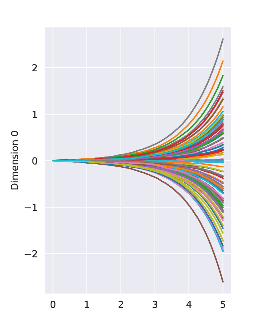
(a) Data

(b) NGM

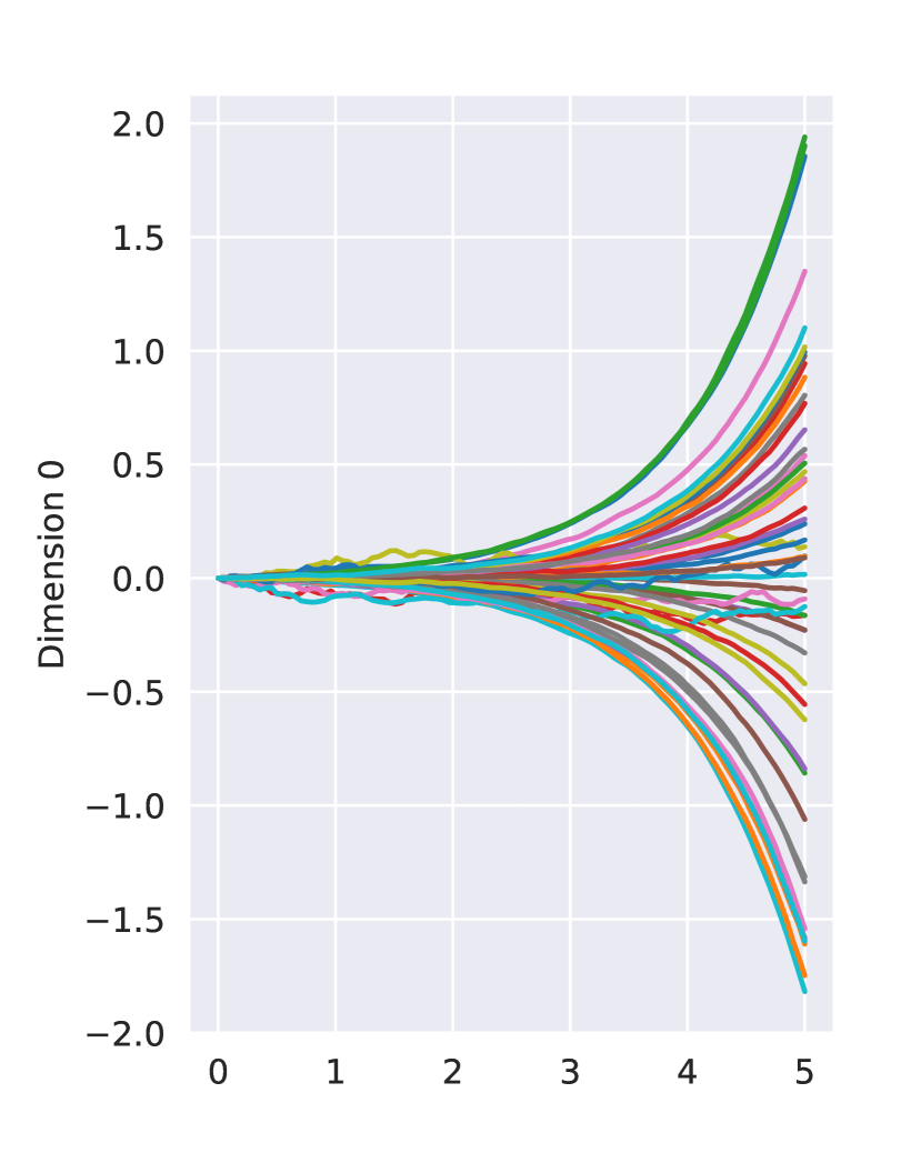
(c) SCOTCH

Figure 2: Comparison between NGM and SCOTCH for simple SDE (note vertical axis scale)

Appendix D Experiments

D.1 Synthetic datasets: Lorenz

D.1.1 Data generation

For the Lorenz dataset, we simulate time-series data according to the following SDE based on the $D$-dimensional Lorenz-96 system of ODEs:

$$dX_{t,d}=((X_{t,d+1}-X_{t,d-2})X_{t,d-1}-X_{t,d})dt+F+\sigma dW_{t,i}$$ (37)

where $X_{t,-1}:=X_{t,D-1},X_{t,0}:=X_{t,D}$, and $X_{t,D+1}:=X_{t,1}$, with parameters set as $F=10$ and $\sigma=0.5$. We generate $N=100$ $10-$dimensional time series, each with length $I=100$, which are sampled with time interval $1$ starting from $t=0$ (that is, $t_{1}=0,t_{2}=1,...,t_{100}=99)$. The initial state $X_{0,i}$ is sampled from a standard Gaussian. To simulate the SDE, we use the Euler-Maruyama scheme with step-size $dt=0.005$.

For this synthetic dataset, we do not add observation noise to the generated time series.

To produce the irregularly sampled versions of the Lorenz dataset, for each time $t=0,...,99$, we randomly drop the observed data at that time with probability $p$, independently at each time $t$ (and for all time series $n=1,...100$). We test using $p=0.3,0.6$ in our experiments.

D.1.2 Hyperparameters

SCOTCH

We use Adam (Kingma and Ba,, 2014) optimizer with learning rate $0.003$ and $0.001$ for $p=0.3$ and $p=0.6$, respectively. We set the $\lambda_{s}=500$ and EM discretization step size $\Delta=1$ for SDE integrator, which coincides with the step size in the data generation process. The time range is set to $[0,100]$. We enable the residual connections for prior drift and diffusion network. We also adopt a learning rate warm-up schedule, where we linearly increase the learning rate from $0$ to the target value within $100$ epochs. We do not mini-batch across the time series. We train $5000$ epochs for convergence.

NGM

We use the same hyperparameter setup as NGM (Bellot et al.,, 2021) where we set $0.1$ for the group lasso regularizer and the learning rate as $0.005$. We train NGM for $4000$ epochs in total ($2000$ for the group lasso stage and $2000$ for the adaptive group lasso stage).

VARLiNGaM

We set the lag to be the same as the ground truth $lag=1$, and do not prune the inferred adjacency matrix.

PCMCI+

We use partial correlation as the underlying conditional independence test. We set the maximum lag at $2$, and let the algorithm itself optimise the significance level. We use the threshold $0.07$ to determine the graph from the inferred value matrix.

CUTS

We use the authors’ suggested hyperparameters (Cheng et al.,, 2023) for the Lorenz dataset.

Rhino

We use hyperparameters with learning rate $0.01$, $70$ epochs of augmented lagrangian training with $6000$ steps each, time lag of $2$, sparsity parameter $\lambda_{s}=5$, and enable instantaneous effects.

D.1.3 Additional results

Figure 3 shows the curve of other metrics.

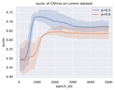
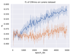
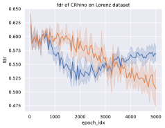
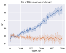
Figure 3: The AUROC (top left), F1 score (top right), false discovery rate (bottom left) and true positive rate (bottom right) curves of SCOTCH for Lorenz dataset. The shaded area indicates the $95\%$ confidence intervals. Blue color indicates the dataset with missing probability $0.3$ and orange color indicates missing probability $0.6$.

D.2 Synthetic datasets: Glycolysis

D.2.1 Data generation

In this synthetic experiment, we generate data according to the system presented by Daniels and Nemenman, (2015), which models a glycolyic oscillator. This is a $D=7$ dimensional system with the following equations:

$$dX_{t,1}=\left(2.5-\frac{100X_{t,1}X_{t,6}}{1+(X_{t,6}/0.52)^{4}}\right)dt+0.01dW_{t,1}$$

$$dX_{t,2}=\left(\frac{200X_{t,1}X_{t,6}}{1+(X_{t,6}/0.52)^{4}}-6X_{t,2}(1-X_{t,5})-12X_{t,2}X_{t,5}\right)dt+0.01dW_{t,2}$$

$$dX_{t,3}=\left(6X_{t,2}(1-X_{t,5})-16X_{t,3}(4-X_{t,6})\right)dt+0.01dW_{t,3}$$

$$dX_{t,4}=\left(16X_{t,3}(4-X_{t,6})-100X_{t,4}X_{t,5}-13(X_{t,4}-X_{t,7})\right)dt+0.01dW_{t,4}$$

$$dX_{t,5}=\left(6X_{t,2}(1-X_{t,5})-100X_{t,4}X_{t,5}-12X_{t,2}X_{t,5}\right)dt+0.01dW_{t,5}$$

$$dX_{t,6}=\left(-\frac{200X_{t,1}X_{t,6}}{1+(X_{t,6}/0.52)^{4}}+32X_{t,3}(4-X_{t,6})-1.28X_{t,6}\right)dt+0.01dW_{t,6}$$

$$dX_{t,7}=\left(1.3(X_{t,4}-X_{t,7})-1.8X_{t,7}\right)dt+0.01dW_{t,7}$$

As with the Lorenz dataset, we simulate $N=100$ time series of length $I=100$, starting at $t=0$ and with time interval $1$. The initial state is sampled uniformly from the ranges $X_{0,1}\in[0.15,1.60],X_{0,2}\in[0.19,2.16],X_{0,3}\in[0.04,0.20],X_{0,4}\in[0.10,0.35],X_{0,5}\in[0.08,0.30],X_{0,6}\in[0.14,2.67],X_{0,7}\in[0.05,0.10]$, as indicated in Daniels and Nemenman, (2015). To simulate the SDE, we use the Euler-Maruyama scheme with step-size $dt=0.005$.

For this synthetic dataset, we do not add observation noise to the generated time series.

D.2.2 Hyperparameters

SCOTCH

We use the same hyperparameter as Lorenz experiments. The only differences are that we use learning rate $0.001$ and set $\lambda_{s}=200$. We train SCOTCH for $30000$ epochs for convergence.

NGM

Since Bellot et al., (2021) did not release the hyperparameters for their glycolysis experiment, we use the default setup in their code. They are the same as the hyperparameters in Lorenz experiments.

VARLiNGaM

Same as Lorenz experiment setup.

PCMCI+

Same as Lorenz experiment setup.

CUTS

Same as Lorenz experiment setup.

Rhino

Same as Lorenz experiment setup.

D.2.3 Additional results

Table 4 shows the performance comparison of SCOTCH to NGM with the original glycolysis data, where the data have different variable scales. We can observe that this difference in scale does not affect the AUROC of SCOTCH but greatly affects NGM. Since AUROC is threshold free, we can see that SCOTCH is more robust in terms of scaling compared to NGM. A possible reason is that the stochastic evolution of the variables in SDE can help stabilise the training when encountering difference in scales, but ODE can easily overshoot due to its deterministic nature.

Figure 4 shows the curves of different metrics. Interestingly, we can see that data normalisation does not improve the AUROC performance (compared to NGM), but does increase the f1 score. This may be because f1 is threshold sensitive and the default threshold of $0.5$ might not be optimal. We can see this through the TPR plot, where ”Original” has very low value.

Table 4: Performance comparison with original Glycolysis data

	AUROC	TPR $\uparrow$	FDR $\downarrow$
SCOTCH	0.7352$\pm$0.019	0.3623$\pm$0.007	0.1575$\pm$0.05
NGM	0.5248$\pm$0.057	0.3478$\pm$0.035	0.4559$\pm$0.094

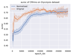
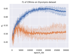
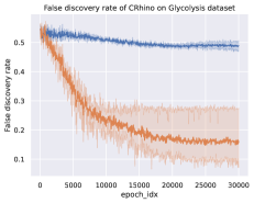
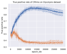
Figure 4: The AUROC (top left), F1 score (top right), false discovery rate (bottom left) and true positive rate (bottom right) curves of SCOTCH for Glycolysis dataset. The shaded area indicates the $95\%$ confidence intervals. Blue color indicates the normalized dataset and orange color indicates the original dataset.

D.3 Dream3 dataset

In this appendix, we will include experiment setups, hyperparameters and additional plots for Dream3 experiment.

D.3.1 Hyperparameters

SCOTCH

We follow similar setup as Lorenz experiment. The differences are that the learning rate is $0.001$. The time range is set to $[0,1.05]$ with EM discretization step size $0.05$, which results in exactly $21$ observations for each time series. We choose sparisty coefficient $\lambda_{s}=200$. For all sub-datasets, we normalize the data to have $0$ mean and unit variance for each dimension. We use the above hyperparameters for Ecoli1, Ecoli2 and Yeast1 sub-datasets. For Yeast2, we only change the learning rate to be $0.0005$. For Yeast3, we change the $\lambda_{s}=50$. We train SCOTCH for $30000$ epochs until convergence.

NGM

For NGM, we follow the same hyperparameter setup as (Cheng et al.,, 2023), where we set the group lasso regulariser as $0.05$, learning rate $0.005$. We train NGM with $4000$ epochs ($2000$ each for group lasso and adaptive group lasso stages). For fair comparison, we use the same observation time (i.e. equally spaced time points within $[1,1.05]$ and step size $0.05$).

PCMCI+ and Rhino

As the experiment setup is the same, we directly cite the number from Gong et al., (2022).

CUTS

We use the authors’ suggested hyperparameters (Cheng et al.,, 2023) for the DREAM3 datasets.

D.3.2 Additional plots

In this section, we include additional metric curves of SCOTCH in fig. 5. Each curve is obtained by averaging over 5 runs and the shaded area indicates the $95\%$ confidence interval. From the value of f1 score, FDR and TPR, we can see DREAM3 is indeed a challenging dataset, where all f1 scores are below 0.5 and FDR only drops to 0.7. From the TPR plot, it is expected to drop at the beginning and then increase during training, which is the case for Ecoli1, Ecoli2 and Yeast1. TPR corresponds well to auroc and f1 score since Ecoli1, Ecoli2 and Yeast1 have much better values compared to Yeast2 and Yeast3.

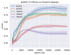
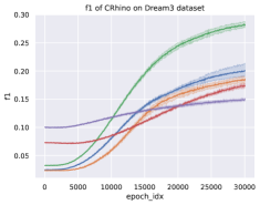
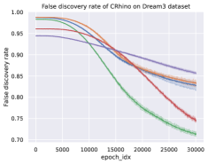
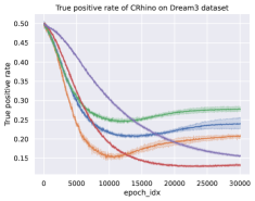
Figure 5: The AUROC (top left), F1 score (top right), false discovery rate (bottom left) and true positive rate (bottom right) curves of SCOTCH for each DREAM3 sub-datasets. The shaded area indicates the $95\%$ confidence intervals.

D.4 Netsim

D.4.1 Experiment setup

For the Netsim dataset, we generate the missing data versions in the same way as the Lorenz dataset (see appendix D.1).

D.4.2 Hyperparameters

SCOTCH

We use similar hyperparameter setup as Dream3 (section D.3.1), but we change $\lambda_{s}=1000$ and use the raw data without normalisation. We train SCOTCH for $10000$ epochs.

NGM

We follow the same setup as DREAM3 experiment, which also coincides with the setup used in Cheng et al., (2023).

PCMCI

We follow the same setup as Lorenz and use threshold $0.07$ to infer the graph.

CUTS

We use the authors’ suggested hyperparameters (Cheng et al.,, 2023) for the Netsim dataset.

Rhino and Rhino+NoInst

we directly cite the number from Gong et al., (2022) for the full dataset, and use the same hyperparameters as Gong et al., (2022) for both $p=0.1$ and $p=0.2$ Netsim datasets.

D.4.3 Additional plots

We include additional metric curves of SCOTCH on Netsim dataset in fig. 6. From the plot, we can see Netsim is a easier dataset compared to DREAM3 since the dimensionality is much smaller. An interesting observation is f1 score does not necessarily correspond well to auroc since f1 score is threshold dependent (by default we use 0.5) but not auroc. To evaluate the robustness of the model, we decide to report AUROC instead of f1 score.

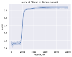
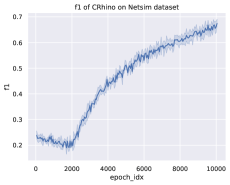
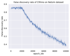
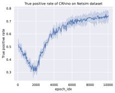
Figure 6: The AUROC (top left), F1 score (top right), false discovery rate (bottom left) and true positive rate (bottom right) curves of SCOTCH for Netsim dataset. The shaded area indicates the $95\%$ confidence intervals.

Appendix E Interventions

Aside from learning the graphical structure between variables, one might also be interested in analysing the effect of applying external changes, or interventions, to the system. Broadly speaking, there are two types of interventions that we can consider in a continuous-time model. The first is to intervene on the dynamics (that is, the drift or diffusion functions), possibly for a set period of time. The second is to directly intervene on the value of (some subset of) variables. The goal is to employ our learned SCOTCH model in order to predict the effect of these interventions on the underlying system.

The former is easy to implement as we need only replace (parts of) the learned drift/diffusion function with the intervention. However, the latter is slightly more subtle than it might first appear. (Hansen and Sokol,, 2014) proposed to define such an intervention as a function that fixes the value of a particular variable as a function of the other variables. However, it is unclear how we can generalize this to interventions affecting more than one variable. For example, a intervention policy $Z_{1}\leftarrow Z_{2},Z_{2}\leftarrow Z_{1}+1$ creats a feedback loop whose semantics are not easy to resolve. Thus, we propose the following definition:

Definition 3 (State-space Intervention).

Given a $D$-dimensional SDE, a state-space intervention is an idempotent function $\iota(t,{\bm{Z}}):\mathbb{R}^{D+1}\to\mathbb{R}^{D}$; that is, $\iota(t,\iota(t,{\bm{Z}}))\equiv\iota(t,{\bm{Z}})$. The corresponding intervened stochastic process is defined by:

$$\tilde{{\bm{Z}}}_{t}=\iota\left(t,\tilde{{\bm{Z}}}_{0}+\sum_{d\in[D]}\int_{0}^{t}{\bm{f}}(\tilde{{\bm{Z}}}_{s})ds+\sum_{d\in[D]}\int_{0}^{t}{\bm{g}}(\tilde{{\bm{Z}}}_{s})d\bm{W}_{s}\right)$$ (38)

The requirement of idempotence captures the intuition that applying the same intervention twice should result in the same result. Some examples of interventions are given as follows:

• Identity: If $\iota(t,{\bm{Z}})={\bm{Z}}\;\forall t\in[T_{1},T_{2}],{\bm{Z}}\in\mathbb{R}^{D}$, then the system evolves accoridng to the original SDE in this time period, with initial state $\tilde{{\bm{Z}}}_{T_{1}}$.

• Ordered Intervention: Given some ordered subset of the variables, we can consider intervening on each variable in order, as a function of the previous variables in the order. That is, we restrict each dimension $\iota_{i}$ of the intervention output to be of the form

  $$\iota_{i}(t,{\bm{Z}}_{t})=\iota_{i}(t,{\bm{Z}}_{t,<i})$$ (39)

  where ${\bm{Z}}_{t,<i}=\{{\bm{Z}}_{t,j}:j<i\}$. It can easily be seen that $\iota$ is always idempotent in this case.

• Projection: Another example of an idempotent function is a projection. This could simulate a setting where external force is applied to ensure the SDE trajectories satisfy spatial constraints. Note that a projection cannot necessarily be expressed as an ordered intervention (e.g. consider projection onto a sphere).

In practice, we implement state-space interventions in SDEs learned from SCOTCH by modifying the SDE solver (e.g. Euler-Maruyama) such that each step is followed with an intervention assignment ${\bm{Z}}_{t}\leftarrow\iota(t,{\bm{Z}}_{t})$.

References

- Amornbunchornvej et al., (2019) Amornbunchornvej, C., Zheleva, E., and Berger-Wolf, T. Y. (2019). Variable-lag granger causality for time series analysis. In 2019 IEEE International Conference on Data Science and Advanced Analytics (DSAA), pages 21–30. IEEE.
- Annadani et al., (2023) Annadani, Y., Pawlowski, N., Jennings, J., Bauer, S., Zhang, C., and Gong, W. (2023). Bayesdag: Gradient-based posterior sampling for causal discovery. arXiv preprint arXiv:2307.13917.
- Assaad et al., (2022) Assaad, C. K., Devijver, E., and Gaussier, E. (2022). Survey and evaluation of causal discovery methods for time series. Journal of Artificial Intelligence Research, 73:767–819.
- Bellot et al., (2021) Bellot, A., Branson, K., and van der Schaar, M. (2021). Neural graphical modelling in continuous-time: consistency guarantees and algorithms. arXiv preprint arXiv:2105.02522.
- Berzuini et al., (2012) Berzuini, C., Dawid, P., and Bernardinell, L. (2012). Causality: Statistical perspectives and applications. John Wiley & Sons.
- Boué and Dupuis, (1998) Boué, M. and Dupuis, P. (1998). A variational representation for certain functionals of brownian motion. The Annals of Probability, 26(4):1641–1659.
- Bracco et al., (2018) Bracco, A., Falasca, F., Nenes, A., Fountalis, I., and Dovrolis, C. (2018). Advancing climate science with knowledge-discovery through data mining. npj Climate and Atmospheric Science, 1(1):20174.
- Bussmann et al., (2021) Bussmann, B., Nys, J., and Latré, S. (2021). Neural additive vector autoregression models for causal discovery in time series. In Discovery Science: 24th International Conference, DS 2021, Halifax, NS, Canada, October 11–13, 2021, Proceedings 24, pages 446–460. Springer.
- Chen et al., (2018) Chen, R. T., Rubanova, Y., Bettencourt, J., and Duvenaud, D. K. (2018). Neural ordinary differential equations. Advances in neural information processing systems, 31.
- Chen et al., (2017) Chen, S., Shojaie, A., and Witten, D. M. (2017). Network reconstruction from high-dimensional ordinary differential equations. Journal of the American Statistical Association, 112(520):1697–1707.
- Cheng et al., (2023) Cheng, Y., Yang, R., Xiao, T., Li, Z., Suo, J., He, K., and Dai, Q. (2023). Cuts: Neural causal discovery from irregular time-series data. arXiv preprint arXiv:2302.07458.
- Cho et al., (2014) Cho, K., Van Merriënboer, B., Gulcehre, C., Bahdanau, D., Bougares, F., Schwenk, H., and Bengio, Y. (2014). Learning phrase representations using rnn encoder-decoder for statistical machine translation. arXiv preprint arXiv:1406.1078.
- Cini et al., (2022) Cini, A., Marisca, I., and Alippi, C. (2022). Filling the g_ap_s: Multivariate time series imputation by graph neural networks. In International Conference on Learning Representations.
- Dang et al., (2019) Dang, X.-H., Shah, S. Y., and Zerfos, P. (2019). seq2graph: Discovering dynamic non-linear dependencies from multivariate time series. In 2019 IEEE International Conference on Big Data (Big Data), pages 1774–1783. IEEE.
- Daniels and Nemenman, (2015) Daniels, B. C. and Nemenman, I. (2015). Efficient inference of parsimonious phenomenological models of cellular dynamics using s-systems and alternating regression. PloS one, 10(3):e0119821.
- Dupuis and Ellis, (2011) Dupuis, P. and Ellis, R. S. (2011). A weak convergence approach to the theory of large deviations. John Wiley & Sons.
- Geffner et al., (2022) Geffner, T., Antoran, J., Foster, A., Gong, W., Ma, C., Kiciman, E., Sharma, A., Lamb, A., Kukla, M., Pawlowski, N., et al. (2022). Deep end-to-end causal inference. arXiv preprint arXiv:2202.02195.
- Goldberger and West, (1987) Goldberger, A. L. and West, B. J. (1987). Applications of nonlinear dynamics to clinical cardiology. Annals of the New York Academy of Sciences, 504:195–213.
- Gong et al., (2022) Gong, W., Jennings, J., Zhang, C., and Pawlowski, N. (2022). Rhino: Deep causal temporal relationship learning with history-dependent noise. arXiv preprint arXiv:2210.14706.
- Gong et al., (2018) Gong, W., Li, Y., and Hernández-Lobato, J. M. (2018). Meta-learning for stochastic gradient mcmc. arXiv preprint arXiv:1806.04522.
- Hansen and Sokol, (2014) Hansen, N. and Sokol, A. (2014). Causal interpretation of stochastic differential equations.
- Hasan et al., (2021) Hasan, A., Pereira, J. M., Farsiu, S., and Tarokh, V. (2021). Identifying latent stochastic differential equations. IEEE Transactions on Signal Processing, 70:89–104.
- He et al., (2016) He, K., Zhang, X., Ren, S., and Sun, J. (2016). Deep residual learning for image recognition. In Proceedings of the IEEE conference on computer vision and pattern recognition, pages 770–778.
- Heltberg et al., (2019) Heltberg, M. L., Krishna, S., and Jensen, M. H. (2019). On chaotic dynamics in transcription factors and the associated effects in differential gene regulation. Nature communications, 10(1):71.
- Hornik et al., (1989) Hornik, K., Stinchcombe, M., and White, H. (1989). Multilayer feedforward networks are universal approximators. Neural networks, 2(5):359–366.
- Hoyer et al., (2008) Hoyer, P., Janzing, D., Mooij, J. M., Peters, J., and Schölkopf, B. (2008). Nonlinear causal discovery with additive noise models. Advances in neural information processing systems, 21.
- Hyvärinen et al., (2010) Hyvärinen, A., Zhang, K., Shimizu, S., and Hoyer, P. O. (2010). Estimation of a structural vector autoregression model using non-gaussianity. Journal of Machine Learning Research, 11(5).
- Khanna and Tan, (2019) Khanna, S. and Tan, V. Y. (2019). Economy statistical recurrent units for inferring nonlinear granger causality. arXiv preprint arXiv:1911.09879.
- Khemakhem et al., (2020) Khemakhem, I., Kingma, D., Monti, R., and Hyvarinen, A. (2020). Variational autoencoders and nonlinear ica: A unifying framework. In International Conference on Artificial Intelligence and Statistics, pages 2207–2217. PMLR.
- Kingma and Ba, (2014) Kingma, D. P. and Ba, J. (2014). Adam: A method for stochastic optimization. arXiv preprint arXiv:1412.6980.
- Li et al., (2020) Li, X., Wong, T.-K. L., Chen, R. T., and Duvenaud, D. (2020). Scalable gradients for stochastic differential equations. In International Conference on Artificial Intelligence and Statistics, pages 3870–3882. PMLR.
- Lorenz, (1996) Lorenz, E. N. (1996). Predictability: A problem partly solved. In Proc. Seminar on predictability, volume 1. Reading.
- Löwe et al., (2022) Löwe, S., Madras, D., Zemel, R., and Welling, M. (2022). Amortized causal discovery: Learning to infer causal graphs from time-series data. In Conference on Causal Learning and Reasoning, pages 509–525. PMLR.
- Marbach et al., (2009) Marbach, D., Schaffter, T., Mattiussi, C., and Floreano, D. (2009). Generating realistic in silico gene networks for performance assessment of reverse engineering methods. Journal of computational biology, 16(2):229–239.
- Øksendal and Øksendal, (2003) Øksendal, B. and Øksendal, B. (2003). Stochastic differential equations. Springer.
- Pamfil et al., (2020) Pamfil, R., Sriwattanaworachai, N., Desai, S., Pilgerstorfer, P., Georgatzis, K., Beaumont, P., and Aragam, B. (2020). Dynotears: Structure learning from time-series data. In International Conference on Artificial Intelligence and Statistics, pages 1595–1605. PMLR.
- Peters et al., (2017) Peters, J., Janzing, D., and Schölkopf, B. (2017). Elements of causal inference: foundations and learning algorithms. The MIT Press.
- Prill et al., (2010) Prill, R. J., Marbach, D., Saez-Rodriguez, J., Sorger, P. K., Alexopoulos, L. G., Xue, X., Clarke, N. D., Altan-Bonnet, G., and Stolovitzky, G. (2010). Towards a rigorous assessment of systems biology models: the dream3 challenges. PloS one, 5(2):e9202.
- Qian et al., (2020) Qian, Z., Alaa, A., Bellot, A., Schaar, M., and Rashbass, J. (2020). Learning dynamic and personalized comorbidity networks from event data using deep diffusion processes. In International Conference on Artificial Intelligence and Statistics, pages 3295–3305. PMLR.
- Qiu et al., (2017) Qiu, X., Mao, Q., Tang, Y., Wang, L., Chawla, R., Pliner, H. A., and Trapnell, C. (2017). Reversed graph embedding resolves complex single-cell trajectories. Nature methods, 14(10):979–982.
- Raia, (2008) Raia, F. (2008). Causality in complex dynamic systems: A challenge in earth systems science education. Journal of Geoscience Education, 56(1):81–94.
- Ramsay et al., (2007) Ramsay, J. O., Hooker, G., Campbell, D., and Cao, J. (2007). Parameter estimation for differential equations: a generalized smoothing approach. Journal of the Royal Statistical Society Series B: Statistical Methodology, 69(5):741–796.
- Reiser, (2022) Reiser, C. (2022). Causal discovery for time series with latent confounders. arXiv preprint arXiv:2209.03427.
- Runge, (2018) Runge, J. (2018). Causal network reconstruction from time series: From theoretical assumptions to practical estimation. Chaos: An Interdisciplinary Journal of Nonlinear Science, 28(7).
- Runge, (2020) Runge, J. (2020). Discovering contemporaneous and lagged causal relations in autocorrelated nonlinear time series datasets. In Conference on Uncertainty in Artificial Intelligence, pages 1388–1397. PMLR.
- Runge et al., (2019) Runge, J., Nowack, P., Kretschmer, M., Flaxman, S., and Sejdinovic, D. (2019). Detecting and quantifying causal associations in large nonlinear time series datasets. Science advances, 5(11):eaau4996.
- Shimizu et al., (2006) Shimizu, S., Hoyer, P. O., Hyvärinen, A., Kerminen, A., and Jordan, M. (2006). A linear non-gaussian acyclic model for causal discovery. Journal of Machine Learning Research, 7(10).
- Shojaie and Michailidis, (2010) Shojaie, A. and Michailidis, G. (2010). Discovering graphical granger causality using the truncating lasso penalty. Bioinformatics, 26(18):i517–i523.
- Siggiridou and Kugiumtzis, (2015) Siggiridou, E. and Kugiumtzis, D. (2015). Granger causality in multivariate time series using a time-ordered restricted vector autoregressive model. IEEE Transactions on Signal Processing, 64(7):1759–1773.
- Spirtes et al., (2000) Spirtes, P., Glymour, C. N., and Scheines, R. (2000). Causation, prediction, and search. MIT press.
- Tank et al., (2021) Tank, A., Covert, I., Foti, N., Shojaie, A., and Fox, E. B. (2021). Neural granger causality. IEEE Transactions on Pattern Analysis and Machine Intelligence, 44(8):4267–4279.
- Trapnell et al., (2014) Trapnell, C., Cacchiarelli, D., Grimsby, J., Pokharel, P., Li, S., Morse, M., Lennon, N. J., Livak, K. J., Mikkelsen, T. S., and Rinn, J. L. (2014). The dynamics and regulators of cell fate decisions are revealed by pseudotemporal ordering of single cells. Nature biotechnology, 32(4):381–386.
- (53) Tzen, B. and Raginsky, M. (2019a). Neural stochastic differential equations: Deep latent gaussian models in the diffusion limit. arXiv preprint arXiv:1905.09883.
- (54) Tzen, B. and Raginsky, M. (2019b). Theoretical guarantees for sampling and inference in generative models with latent diffusions. In Conference on Learning Theory, pages 3084–3114. PMLR.
- Welling and Teh, (2011) Welling, M. and Teh, Y. W. (2011). Bayesian learning via stochastic gradient langevin dynamics. In Proceedings of the 28th international conference on machine learning (ICML-11), pages 681–688. Citeseer.
- Wu et al., (2014) Wu, H., Lu, T., Xue, H., and Liang, H. (2014). Sparse additive ordinary differential equations for dynamic gene regulatory network modeling. Journal of the American Statistical Association, 109(506):700–716.
- Wu et al., (2020) Wu, T., Breuel, T., Skuhersky, M., and Kautz, J. (2020). Discovering nonlinear relations with minimum predictive information regularization. arXiv preprint arXiv:2001.01885.
- Xu et al., (2019) Xu, C., Huang, H., and Yoo, S. (2019). Scalable causal graph learning through a deep neural network. In Proceedings of the 28th ACM international conference on information and knowledge management, pages 1853–1862.
- Zhang et al., (2018) Zhang, C., Bütepage, J., Kjellström, H., and Mandt, S. (2018). Advances in variational inference. IEEE transactions on pattern analysis and machine intelligence, 41(8):2008–2026.
- Zhang et al., (2017) Zhang, K., Huang, B., Zhang, J., Glymour, C., and Schölkopf, B. (2017). Causal discovery from nonstationary/heterogeneous data: Skeleton estimation and orientation determination. In IJCAI: Proceedings of the Conference, volume 2017, page 1347. NIH Public Access.
- Zheng et al., (2018) Zheng, X., Aragam, B., Ravikumar, P. K., and Xing, E. P. (2018). Dags with no tears: Continuous optimization for structure learning. Advances in neural information processing systems, 31.