Combinatorics of nondeterministic walks

Abstract

This paper introduces nondeterministic walks, a new variant of one-dimensional discrete walks. The main difference to classical walks is that its nondeterministic steps consist of sets of steps from a predefined set such that all possible extensions are explored in parallel. We discuss in detail the nondeterministic Dyck step set $\{\{-1\},\{1\},\{-1,1\}\}$ and Motzkin step set $\{\{-1\},\{0\},\{1\},\{-1,0\},\{-1,1\},\{0,1\},\{-1,0,1\}\}$, and show that several nondeterministic classes of lattice paths, such as nondeterministic bridges, excursions, and meanders are algebraic. The key concept is the generalization of the ending point of a walk to its reachable points, i.e., a set of ending points. We extend our results to general step sets: We show that nondeterministic bridges and several subclasses of nondeterministic meanders are always algebraic. We conjecture the same is true for nondeterministic excursions, and we present python and Maple packages to support our conjecture.

This research is motivated by the study of networks involving encapsulation and decapsulation of protocols. Our results are obtained using generating functions, analytic combinatorics, and additive combinatorics.

Keywords. Random walks, analytic combinatorics, generating functions, limit laws, networking, encapsulation.

1 Introduction

In recent years, lattice paths have received a lot of attention in different fields, such as probability theory, computer science, biology, chemistry, and physics [24, 21, 12, 6]. One of their key features is their versatility as models to capture natural phenomena, as in up-to-date models of certain polymers [23]. In this paper we continue this success story and present a new model of lattice paths capturing the en- and decapsulation of protocols over networks. The key to understand them will be to be able to follow all trajectories in the network simultaneously. For this purpose, we generalize the class of lattice paths to so called nondeterministic lattice paths. In our context, this word does not mean “random”. Instead it is understood in the same sense as for automata and Turing machines. A process is nondeterministic if several branches are explored in parallel, and the process is said to end in an accepting state if one of those branches ends in an accepting state. Before we give a precise definition, we recall the classical model of lattice we build on [2].

Classical walks.

Given a finite set $S\subset\mathds{Z}$ of integers, called the steps, a walk of length $n$ is a sequence $v=(v_{1},\ldots,v_{n})$ of steps $v_{i}\in S$. In this paper we will always assume that our walks start at the origin. Its its endpoint is equal to the sum of its steps $\sum_{i=1}^{n}v_{i}$. As illustrated in Figure 1a, a walk can be visualized by its geometric realization as a sequence of ordinates $(y_{0},y_{1},\dots,y_{n})$. Since the walk starts at the origin it starts at $y_{0}=0$, and after appending $k$ steps it has reached $y_{k}:=\sum_{i=1}^{k}v_{i}$. Thus, the relation $v_{i}=y_{i}-y_{i-1}$ directly connects the steps and the ordinates of a walk, and shows their equivalence.

We distinguish four different types of walks:

• A bridge is a walk with endpoint $y_{n}=0$.

• A meander is a walk never crossing the $y$-axis, i.e., $y_{j}\geq 0$ for all $j=0,\ldots,n$.

• An excursion is a meander with endpoint $y_{n}=0$.

Nondeterministic walks.

We are now ready to generalize classical walks to nondeterministic walks. The only difference to above is that steps are now sets of integers.

Definition 1.1 (Nondeterministic walks).

An N-step $s\subset\mathds{Z}$ is a non-empty finite set of integers. Given an N-step set $S=\{s_{1},\ldots,s_{m}\}$ of N-steps, an N-walk of length $n$ is a sequence $(s_{1},\dots,s_{n})$ of N-steps $s_{i}\in S$.

In addition, as for classical walks, we always assume that they start at the origin and we distinguish different families.

Definition 1.2 (Families of N-walks).

An N-walk $w=(w_{1},\ldots,w_{n})$ and a classical walk $v=(v_{1},\ldots,v_{n})$ are compatible if they have the same length $n$, the same starting point, and for each $1\leq i\leq n$, the $i^{\text{th}}$ step is included in the $i^{\text{th}}$ N-step, i.e., $v_{i}\in w_{i}$. An N-bridge (resp. N-meander, resp. N-excursion) is an N-walk compatible with at least one bridge (resp. meander, resp. excursion). Thus, N-excursions are particular cases of N-meanders.

The endpoints of classical walks are central to the analysis. We define their nondeterministic analogues.

Definition 1.3 (Reachable points).

The reachable points of an N-walk (resp. N-meanders) are the endpoints of all compatible walks (resp. meanders). The minimum (resp. maximum) reachable point of an N-walk $w$ is denoted by $\min(w)$ (resp. $\max(w)$). The minimum (resp. maximum) reachable point of an N-meander $w$ is denoted by $\min^{+}(w)$ (resp. $\max^{+}(w)$).

Note that the reachable endpoints of an N-meander are nonnegative. The geometric realization of an N-walk is the sequence of its reachable points after $j$ steps for $j=0,\dots,n$, as shown in Figure 1.

(a) A classical walk.

(b) An N-walk.

(c) Meanders compatible with the N-walk.

Figure 1: Geometric realization of the classical meander $v=(2,-1,0,1)$, the N-walk $w=\left(\{2\},\{-1,1\},\{-2,0\},\{0,1,2\}\right)$, and the N-meander with the same N-steps. As highlighted in red, $v$ is compatible with $w$.

Moreover, the steps of a walks or N-walk can be weighted. Then, each step is associated with a weight $p_{i}$ and the weight of the N-walk is the product of the weights associated to its steps. In many cases, these weights $p_{i}$ will represent probabilities, i.e., $p_{i}\geq 0$ and $p_{1}+\dots+p_{m}=1$. We talk about the unweighted model when all weights are equal to one: $p_{i}=1$.

1.1 Main results

Our main results are the analysis of the asymptotic number of nondeterministic walks of the Dyck and Motzkin type with step sets

$$\Big{\{}\{-1\},\{1\},\{-1,1\}\Big{\}}\qquad\text{ and }\qquad\Big{\{}\{-1\},\{0\},\{1\},\{-1,0\},\{-1,1\},\{0,1\},\{-1,0,1\}\Big{\}},$$

respectively. The results for the unweighted case are summarized in Table 1. These results are derived using generating functions and singularity analysis. Remarkably, for N-bridges, N-meanders, and N-excursions the leading order compared to the lower order terms are of different order of magnitude. This phenomenon arises due to a dominant polar singularity followed by a square root singularity. Moreover, observe that for different types the leading orders only differ in the multiplicative constants. This is in sharp contrast to classical walks, in which we observe polynomial differences [2]. For example the number of classical bridges of size $n$ are of order $o(\sqrt{n})$ compared to classical walks. Here, this polynomial change in order of magnitude is only visible in the lower order terms. In particular, the limit probabilities for a Dyck N-walk of even length to be an N-bridge, an N-meander, or an N-excursion, are $1$, $\frac{1}{2}$, or $\frac{1}{4}$, and for Motzkin N-walks $1$, $\frac{3}{4}$, or $\frac{9}{16}$, respectively.

We also explore general N-steps and prove that the generating function of N-bridges with respect to length, minimal, and maximal reachable point is always algebraic in Theorem 4.1. We conjecture that the generating function of N-excursions is always algebraic and provide proofs in some specific cases in Section 5.

Type	Dyck N-steps	Motzkin N-steps
	$\mathcal{P}(\{-1,1\})\setminus\emptyset$	$\mathcal{P}(\{-1,0,1\})\setminus\emptyset$
N-Walk	$3^{n}$	$7^{n}$
N-Bridge	$\frac{1+(-1)^{n}}{2}\left(3^{n}-\frac{2\sqrt{2}}{\sqrt{\pi}}\frac{8^{n/2}}{\sqrt{n}}+\mathcal{O}\left(\frac{8^{n/2}}{n^{3/2}}\right)\right)$	$7^{n}-\sqrt{\frac{3}{\pi}}\frac{6^{n}}{\sqrt{n}}+\mathcal{O}\left(\frac{6^{n}}{n^{3/2}}\right)$
N-Meander	$\frac{3^{n}}{2}+\frac{3\sqrt{2}(1+(-1)^{n})+4(1-(-1)^{n})}{\sqrt{\pi}}\frac{8^{n/2}}{\sqrt{n^{3}}}+\mathcal{O}\left(\frac{8^{n/2}}{n^{5/2}}\right)$	$\frac{3}{4}7^{n}+\frac{3\sqrt{3}}{2\sqrt{\pi}}\frac{6^{n}}{\sqrt{n^{3}}}+\mathcal{O}\left(\frac{6^{n}}{n^{5/2}}\right)$
N-Excursion	$\frac{1+(-1)^{n}}{2}\left(\frac{3^{n}}{4}+4\sqrt{2}\frac{8^{n/2}}{\sqrt{\pi n^{3}}}+\mathcal{O}\left(\frac{8^{n/2}}{n^{5/2}}\right)\right)$	$\frac{9}{16}7^{n}-\gamma\frac{6^{n}}{\sqrt{\pi n^{3}}}+\mathcal{O}\left(\frac{6^{n}}{n^{5/2}}\right)$

Table 1: The asymptotic number of nondeterministic unweighted (all weights equal to one) Dyck and Motzkin N-walks, N-brdiges, N-meanders, and N-excursions with $n$ steps. The constant $\gamma\approx 0.6183$ is an algebraic number defined as the positive real solution of $1024\gamma^{4}-8019\gamma^{2}+2916=0$.

1.2 Motivation and related work

Our nondeterministic model of lattice paths has its roots in networking. Let us first give a vivid description of the underlying mechanisms using Russian dolls.

Russian dolls.

Suppose we have a set of $n+1$ people arranged in a line. There are three kinds of people. A person of the first kind is only able to put a received doll in a bigger one. A person of the second kind is only able to extract a smaller doll (if any) from a bigger one. If she receives the smallest doll, then she throws it away. Finally, a person of the third kind can either put a doll in a bigger one or extract a smaller doll if any. We want to know if it is possible for the last person to receive the smallest doll after it has been given to the first person and then, consecutively, handed from person to person while performing their respective operations. This is equivalent to asking if a given N-walk with each N-step $\in\left\{\{1\},\{-1\},\{-1,1\}\right\}$ is an N-excursion, i.e., if the N-walk is compatible with at least one excursion. The probabilistic version of this question is: what is the probability that the last person can receive the smallest doll according to some distribution on the set of people over the three kinds?

Networks and encapsulations.

The original motivation of this work comes from networking. In a network, some nodes are able to encapsulate protocols (put a packet of a protocol inside a packet of another one), decapsulate protocols (extract a nested packet from another one), or perform any of these two operations (albeit most nodes are only able to transmit packets as they receive them). Typically, a tunnel is a subpath starting with an encapsulation and ending with the corresponding decapsulation. Tunnels are very useful for achieving several goals in networking (e.g., interoperability: connecting IPv6 networks across IPv4 ones [33]; security and privacy: securing IP connections [30], establishing Virtual Private Networks [29], etc.). Moreover, tunnels can be nested to achieve several goals. Replacing the Russian dolls by packets, it is easy to see that an encapsulation can be modeled by a $\{1\}$-step and a decapsulation by a $\{-1\}$-step, while a passive transmission of a packet is modeled by a $\{0\}$-step.

Given a network with some nodes that are able to encapsulate or decapsulate protocols, a path from a sender to a receiver is feasible if it allows the latter to retrieve a packet exactly as dispatched by the sender. Computing the shortest feasible path between two nodes is polynomial [25] if cycles are allowed without restriction. In contrast, the problem is $\mathsf{NP}$-hard if cycles are forbidden or arbitrarily limited. In [25], the algorithms are compared through worst-case complexity analysis and simulation. The simulation methodology for a fixed network topology is to make encapsulation (resp. decapsulation) capabilities available with some probability $p$ and observe the processing time of the different algorithms. It would be interesting, for simulation purposes, to generate random networks with a given probability of existence of a feasible path between two nodes. This work is the first step towards achieving this goal, since our results give the probability that any path is feasible (i.e., is a N-excursion) according to a probability distribution of encapsulation and decapsulation capabilities over the nodes.

Lattice paths.

Nondeterministic walks naturally connect between lattice paths and branching processes. This is underlined by our usage of many well-established analytic and algebraic tools previously used to study lattice paths. In particular, those are the robustness of D-finite functions with respect to the Hadamard product, and the kernel method [19, 11, 2, 7, 3].

The N-walks are nondeterministic one-dimensional discrete walks. We will see that their generating functions require three variables: one marking the lowest point $\min(w)$ that can be reached by the N-walk $w$, another one marking the highest point $\max(w)$, and the last one marking its length. For this reason they are also closely related to two-dimensional lattice paths, when interpreting $\left(\min(w),\max(w)\right)$ as coordinates in the plane.

Nondeterminism and context-free grammars.

Nondeterministic walks are very closely linked to nondeterministic finite automata and context free grammars. In particular, for any finite set of N-steps the class of N-excursions, N-meanders, and N-bridges can be encoded by a context-free grammar. To see this, note that languages generated by context-free grammars are equivalently recognized by pushdown automata with a single stack. These automata are by definition nondeterministic, hence they allow epsilon transitions which we use to follow all trajectories in the N-walk simultaneously. Then the stack is used to keep track of the distance of the current trajectory to the $x$-axis, thereby distinguishing between different types of N-walks.

If a context-free language admits an unambiguous grammar, the generating function of the number of its words of length $n$ is algebraic. These words of length $n$ are exactly the N-walks of length $n$, and hence, this gives a strong hint that the N-walks we analyze in this paper are algebraic. However, it is not obvious how to find a non-ambiguous grammar directly, and even if it is found, how to derive the characterizing algebraic equations. Moreover, the associated system of equation is already for small examples nearly impossible to solve (resultants of large degree). For this reason, we show in this article an alternative approach for the enumeration and asymptotics building on the “kernel method”. It has the advantage that it captures the algebraic nature of the generating functions and allows to compute the asymptotics via singularity analysis.

We leave as an interesting open problem to determine which N-step sets $S$ correspond to non-ambiguous context free languages for N-bridges or N-excursions.

1.3 Outline of the paper

We start in Section 2 with the analysis of Dyck N-walks. We derive closed forms for the generating functions and two limit laws for reachable points in N-excursions: maximal value at the end and the frequency of $\{0\}$. We continue in Section 3 with the analysis of Motzkin N-walks and derive functional equations and closed forms for special cases. All these computations are made explicit in an accompanying Maple worksheet. In Section 4 we show that the generating function of N-bridges (with respect to length, maximal and minimal reachable point) is algebraic for any finite N-step set using concepts from additive combinatorics. In Section 5 we show that the generating function of N-meanders (with respect to length and maximal reachable point) is also algebraic for any finite N-step set and we conjecture that the same is true for N-excursions. We also present python code that we implemented to derive the functional equations for any N-step set for N-excursion and N-bridges.

This paper is the full version of an extended abstract [15] of 12 pages that was published in the proceedings of the Sixteenth Workshop on Analytic Algorithmics and Combinatorics (ANALCO) in 2019 in San Diego. Here we give all proofs that partly have only been sketched so far. We greatly extend the proof on the algebraicity of general N-bridges in Section 4.2, particularly giving an extended definition of types and the finiteness of the automaton. We additionally give limit law result for Dyck N-walks in Section 2.3 and show results on subclass of general N-excursions in Section 5 and our python package.

2 Dyck N-walks

One of the most fundamental families of classical lattice paths are Dyck paths, which are excursions associated to the step set $\{-1,1\}$. They are enumerated by the ubiquitous Catalan numbers, which also enumerate many other combinatorial objects. In this section we study their corresponding N-walks. A Dyck N-walks is an N-walk associated with the N-step set

$$S_{D}=\Big{\{}\{-1\},\{1\},\{-1,1\}\Big{\}}.$$

Additionally, every step is associated with a weight $p_{-1},p_{1}$, and $p_{-1,1}$, respectively. In the following we will talk of Dyck N-meanders, Dyck N-bridges, and Dyck N-excursions if the walks use the above N-step $S_{D}$ and are N-meanders, N-bridges, or N-excursions, respectively.

2.1 Dyck N-walks and N-bridges

In order to enumerate any class of Dyck N-walks we need to study their reachable points.

Lemma 2.1.

The reachable points of a Dyck N-walk $w$ are

$$\left\{\min(w)+2i\ |\ i\in\left\{0,\dots,\frac{\max(w)-\min(w)}{2}\right\}\right\}.$$

The same result holds for Dyck N-meanders, with $\min(w)$ and $\max(w)$ replaced by $\min^{+}(w)$ and $\max^{+}(w)$; see Definition 1.3.

Proof.

We perform an induction on the number of steps. A walk starts at $0$. After appending a new N-step the reachable points are either shifted down or up by one unit by $\{-1\}$ or $\{1\}$, respectively, or they are the sum of both shifts by $\{-1,1\}$. Hence, there is always a distance $2$ between the reachable points. ∎

By Lemma 2.1 the reachable points are fully determined by their minimum and maximum. Therefore, we define the generating functions $D(x,y;t)$ and $D^{+}(x,y;t)$, of Dyck N-walks and Dyck N-meanders, respectively, as

$$D(x,y;t) :=\sum_{\text{Dyck N-walk $w$}}\bigg{(}\prod_{s\in w}p_{s}\bigg{)}x^{\min(w)}y^{\max(w)}t^{|w|},$$

$$D^{+}(x,y;t) :=\sum_{\text{Dyck N-meander $w$}}\bigg{(}\prod_{s\in w}p_{s}\bigg{)}x^{\min^{+}(w)}y^{\max^{+}(w)}t^{|w|}.$$

Note that by construction these are power series in $t$ with Laurent polynomials in $x$ and $y$, as each of the finitely many N-walks of length $n$ has a finite minimum and maximum reachable point.

Remark 2.2.

The variables $x$ and $y$ are called catalytic variables, as they facilitate the enumeration of such paths by length but are not part of the initial enumeration question. The reachable points used here are a generalization of the coordinate of the end point that is used for classical lattice paths; see, e.g., [2, 10].

As a direct corollary of Lemma 2.1, all N-bridges and N-excursions have even length. The number of Dyck N-bridges and Dyck N-excursions are then, respectively, given by

$$[x^{\leq 0}y^{\geq 0}t^{2n}]D(x,y;t)\qquad\text{and}\qquad[t^{2n}]D^{+}(0,1;t),$$ (1)

where the nonpositive part extraction operator $[x^{\leq 0}]$ is defined as $[x^{\leq 0}]\sum_{k\in\mathbb{Z}}f_{k}x^{k}:=\sum_{k\leq 0}f_{k}x^{k}$ (and analogously for $[y^{\geq 0}]$). In the following two subsections we derive closed-form expressions for these quantities. The generating function of Dyck N-walks has a particularly simple shape.

Proposition 2.3.

The generating function of Dyck N-walks is given by

$$D(x,y;t)=\frac{1}{1-t\left(\frac{p_{-1}}{xy}+p_{1}xy+p_{-1,1}\frac{y}{x}\right)}.$$ (2)

Proof.

The only N-walk of length $0$ is the empty walk. We obtain each non-empty N-walk, by appending an N-step to another N-walk. In terms of generating functions this gives $D(x,y;t)=1+tD(x,y;t)\left(\frac{p_{-1}}{xy}+p_{1}xy+p_{-1,1}\frac{y}{x}\right),$ which proves the claim. ∎

The representation (2) has a direct bijective interpretation in terms of two-dimensional lattice paths. The idea is to interpret the change in the minimum and maximum of the reachable points, as a change in the $x$- and $y$-direction. We get the following mapping from N-steps to 2D-steps.

$$\{-1\} \mapsto(-1,-1), \{1\} \mapsto(1,1), \{-1,1\} \mapsto(-1,1).$$ (3)

To finalize the bijection, we map the origin to the origin. An example of this bijection is shown in Figure 2. This bijection will help us to study N-meanders and N-excursions in the next section.

(a) A Dyck N-walk.

(b) The corresponding $2$D lattice path.

Figure 2: The bijection of Dyck N-walks to two-dimensional lattice paths transforms the N-steps $\{-1\},\{1\},\{-1,1\}$ into the steps $(-1,-1),(1,1),(-1,1)$, respectively.

We now turn our attention to Dyck N-bridges. Their generating function is defined as

$$B(x,y,t)=\sum_{n,k,\ell\geq 0}b_{n,k,\ell}x^{-k}y^{\ell}t^{n}.$$

Recall from Lemma 2.1 that bridges have to be of even length, i.e., $[t^{2n+1}]B(x,y,t)=0$. Moreover, by (1) they are linked to the generating function of N-walks as follows $[t^{2n}]B(x,y,t)=[x^{\leq 0}y^{\geq 0}t^{2n}]D(x,y;t).$ In the following theorem we will reveal a great contrast to classical walks: nearly all N-walks are N-bridges.

Theorem 2.4.

The generating function of Dyck N-bridges $B(x,y,t)$ is algebraic of degree $4$. For $p_{-1}=p_{1}=p_{-1,1}=1$ the generating function of unweighted Dyck N-bridges is algebraic of degree $2$:

$$B(1,1,t) =\frac{1-6t^{2}}{\sqrt{1-8t^{2}}(1-9t^{2})}=1+7t^{2}+63t^{4}+583t^{6}+5407t^{8}+\ldots.$$

The number $[t^{n}]B(1,1,t)$ of unweighted Dyck N-bridges is asymptotically equal to

$$\frac{1+(-1)^{n}}{2}\left(3^{n}-\frac{2\sqrt{2}}{\sqrt{\pi}}\frac{8^{n/2}}{\sqrt{n}}+\mathcal{O}\left(\frac{8^{n/2}}{n^{3/2}}\right)\right).$$

Proof.

In order to improve readability we drop the parity condition on $t$ and define

$$B_{2}(x,y,t):=[x^{\leq 0}y^{\geq 0}]D(x,y;t).$$

Then, $[t^{2n}]B_{2}(x,y,t)=[t^{2n}]B(x,y,t)$, while in general $[t^{2n+1}]B_{2}(x,y,t)\neq 0$ and is therefore not equal to $[t^{2n+1}]B(x,y,t)$. The key observation is the following link between N-bridges and N-walks: An N-bridge is an N-walk whose minimum is neither strictly positive, nor is its maximum strictly negative. This gives

$$\begin{aligned} B_{2}(x,y,t)&=D(x,y;t)-[x^{>0}]D(x,y,t)-[y^{<0}]D(x,y,t).\end{aligned}$$ (4)

Note that in general we would need to correct the right-hand side by $[x^{>0}y^{<0}]D(x,y,t)$, which is however equal to zero by construction, as the minimum can never be larger than the maximum. Recall that $D(x,y,t)$ has a rational closed form given in (2) that admits a bijective interpretation in terms of two-dimensional lattice paths. Then, Equation (4) means that the 2D-walk has to end in the fourth quadrant. To simplify the remaining discussion we introduce the following shorthand:

$$F(x,y,t) :=[x^{>0}]D(x,y,t) G(x,y,t) :=[y^{<0}]D(x,y,t).$$ and

Then, $F(x,y,t)$ corresponds to 2D-walks ending in the right half-plane, and $G(x,y,t)$ to 2D-walks ending in the upper half-plane. Now, the theory of formal Laurent series with positive coefficients (which applies to these problems) implies automatically that they are algebraic. Therefore, the generating function of bridges is algebraic; see e.g., [20, Section 6] which also gives further historical references.

It remains to compute the generating functions explicitly. First, observe that due to the symmetry of the step set we have $F(x,y,t)=G(1/y,1/x,t)$ after additionally interchanging the role of $p_{-1}$ and $p_{1}$. Thus, it suffices to compute $F(x,y,t)$. Following [11], this can be achieved by computing the roots of the denominator of $D(x,y,t)$ and performing a partial fraction decomposition. Note that $D(x,y,t)$ is formal power series in $t$ with Laurent polynomial coefficients in $x$ and $t$, i.e., $D(x,y,t)\in\mathbb{Q}[x,1/x,y,1/y][[t]]$. These computations are performed in the accompanying Maple worksheet. ∎

2.2 Dyck N-meanders and N-excursions

We continue by deriving a functional equation for Dyck N-meanders using a recursive step-by-step decomposition.

Proposition 2.5.

The generating function of Dyck N-meanders is characterized by the relation

$$D^{+}(x,y;t)=1 +t\left(p_{-1}x^{-1}y^{-1}+p_{1}xy+p_{-1,1}x^{-1}y\right)\left(D^{+}(x,y;t)-D^{+}(0,y;t)\right)$$

$$+t\left(p_{-1}xy^{-1}+(p_{1}+p_{-1,1})xy\right)\left(D^{+}(0,y;t)-D^{+}(0,0;t)\right)$$ (5)

$$+t\left(p_{1}+p_{-1,1}\right)xyD^{+}(0,0;t).$$

Proof.

Applying the symbolic method (see [19]), we translate the following combinatorial characterization of N-meanders into the claimed equation. An N-meander is either of length $0$, or it can be uniquely decomposed into an N-meander $w$ followed by an N-step.

If $\min^{+}(w)>0$ then any N-step can be appended. The generating function of N-meanders with positive minimum reachable point is $D^{+}(x,y;t)-D^{+}(0,y;t)$. If $\min^{+}(w)=0$ but $\max^{+}(w)>0$, which corresponds to the generating function $D^{+}(0,y;t)-D^{+}(0,0;t)$, then an additional N-step $\{-1\}$ increases $\min^{+}(w)$ (the path ending at $0$ disappears, and the one ending at $2$ becomes the minimum) and decreases $\max^{+}(w)$, while an additional N-step $\{1\}$ or $\{-1,1\}$ increases both $\min^{+}(w)$ and $\max^{+}(w)$. Finally, if $\min^{+}(w)=\max^{+}(w)=0$, which corresponds to the generating function $D^{+}(0,0;t)$, then the N-step $\{-1\}$ is forbidden, and the two other available N-steps both increase $\min^{+}(w)$ and $\max^{+}(w)$. ∎

The representation (5) admits again an interpretation in terms of two-dimensional lattice paths. For this purpose, we use the bijection (3) and add spatial constraints: The $x$-axis acts as an absorbing barrier, while the $y$-axis as a reflecting one; see Figure 3. This ensures that all paths stay in the first quadrant. In particular, N-excursions are mapped to walks that end on the nonnegative $y$-axis.

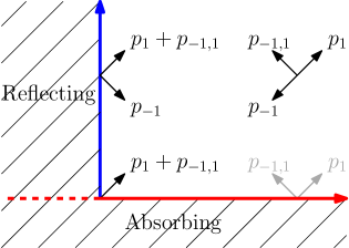
Figure 3: An N-Dyck meander corresponds to a two-dimensional walk with an absorbing $x$-axis and a reflecting (half) $y$-axis and jump polynomial $S(x,y)=p_{1}xy+p_{-1,1}\frac{y}{x}+\frac{p_{-1}}{xy}$.

There is a rich literature on such two-dimensional models and variations. Most variations make the problem much more complicated and often change the nature of the generating function. It is known that the generating function of the same steps as above with both barriers being absorbing is algebraic [11], while there are other cases where it does not even satisfy a (linear) differential equation [28, 16]. Furthermore, one can add weights to the steps [14], but also let the path accumulate weights every time it touches one of the axes [8, 31, 9]. However, for the problem of a changing step sets depending on the current spatial position not much is known. Recently, the problem where the position depends on a nondeterministic automaton was treated for some special cases in [13], yet this does not fit into our framework above. Only in a one-dimensional setting with an absorbing or reflecting barrier it was shown that the generating functions are always algebraic [5]. Since this step set is with respect to the spatial constraints only one-dimensional ($x$-positivity implies $y$-positivity), we expect a similar result. Yet, the result does not follow directly, as there are several boundary constraints and not just one here.

Let us introduce the min-max-change polynomial $S(x,y)$ and the kernel $K(x,y)$:

$$\begin{aligned} S(x,y)&:=\frac{p_{-1}}{xy}+p_{1}xy+p_{-1,1}\frac{y}{x},\\ K(x,y)&:=xy(1-tS(x,y)).\end{aligned}$$ (6)

The generating function of Dyck N-walks admits now the compact form

$$D(x,y;t)=\frac{1}{1-tS(x,y)}.$$ (7)

Remark 2.6 (N-walks for general step sets).

Note that for any finite N-step set $S$ where each step $s\in S$ has weight $p_{s}$, we can define the min-max-change polynomial $S(x,y)$ analogously:

$$S(x,y) =\sum_{s\in S}p_{s}\,x^{\min(s)}y^{\max(s)}.$$

Then, equation (7) for the generating function of N-walks with this step set stays valid, as each N-walk is simply the (unconstrained) concatenation of N-steps.

A key role in the following result on the closed form of Dyck N-meanders is played by $Y(t)$ and $X(y,t)$, the unique power series solutions satisfying $K(1,Y(t))=0$, and $K(X(y,t),y)=0$ which have the following closed forms

$$\begin{aligned} Y(t)&=\frac{1-\sqrt{1-4p_{-1}(p_{1}+p_{-1,1})t^{2}}}{2(p_{1}+p_{-1,1})t},\\ X(y,t)&=\frac{1-\sqrt{1-4p_{1}(p_{-1}+p_{-1,1}y^{2})t^{2}}}{2p_{1}yt}.\end{aligned}$$ (8)

Theorem 2.7.

The generating function $D^{+}(x,y;t)$ of Dyck N-meanders is algebraic of degree $4$ (and degree $2$ for any $p_{i}=0$), and equal to

$$D^{+}(x,y;t) =\begin{cases}\frac{x-X(y,t)}{1-X(y,t)^{2}}\frac{y-xY(t)-X(y,t)Y(t)+xyX(y,t)}{xy(1-tS(x,y))},&\text{ for }p_{1}>0,\\ \frac{y^{2}-xyY(t)+t(p_{-1,1}y^{2}+p_{-1})(Y(t)-xy)}{y^{2}-t^{2}(p_{-1,1}y^{2}+p_{-1})^{2}},&\text{ for }p_{1}=0.\end{cases}$$

The generating functions $D^{+}(1,y,t)$ and $D^{+}(0,0,t)$ are algebraic of degree $2$. The generating function $D^{+}(0,1;t)$ of Dyck N-excursions is algebraic of degree $4$ (degree $2$ for $p_{1}=p_{-1})$.

Proof.

Using the kernel $K(x,y)$ from (6), we first rewrite the functional equation (5) into

$$K(x,y)D^{+}(x,y;t)=xy+t(x^{2}-1)(p_{-1,1}y^{2}+p_{-1})D^{+}(0,y;t)-tx^{2}p_{-1}D^{+}(0,0;t).$$

We observe that after substituting $x=1$ the unknown $D^{+}(0,y;t)$ vanishes, and we are left with the equation

$$K(1,y)D^{+}(1,y;t)=y-tp_{-1}D^{+}(0,0;t).$$

Now, we can use the kernel method (see, e.g., [2]): Substituting $y=Y(t)$ from (8), sets the left-hand side to zero, and allows us to solve for $D^{+}(0,0;t)$. This is legitimate, as $D^{+}(x,y;t)$ is a power series in $t$ with polynomial coefficients in $x$ and $y$. We get

$$D^{+}(0,0;t)=\frac{Y(t)}{p_{-1}t}\qquad\text{ and }\qquad D^{+}(1,y;t)=\frac{y-Y(t)}{K(1,y)}.$$ (9)

Hence, these two generating functions are algebraic of degree $2$. After substituting these results back into the initial equation we apply the kernel method again with respect to the variable $x$. Substituting now $x=X(y,t)$ from (8) we find a closed-form solution for $D^{+}(0,y;t)$. Note that for $p_{1}>0$ the kernel is quadratic in $x$, while for $p_{1}=0$ it is linear. Combining these results proves the claim on $D^{+}(x,y;t)$. From this expression, we directly get the generating function $D^{+}(x,y;t)$ of N-excursions, and a short computation in a computer algebra system like Maple shows the claimed algebraic degree. All mentioned computations can be found in the accompanying Maple worksheet. ∎

Note that by construction of N-meanders, if the maximum of the reachable points is $0$ also the minimum is $0$. In terms of generating functions, we have $D^{+}(x,0;t)=D^{+}(0,0;t)$.

Remark 2.8 (Case $p_{1}=0$).

The closed form for $D^{+}(x,y;t)$ in the case of $p_{1}=0$ is the same as the limit $p_{1}\to 0$ of the form $p_{1}>0$. Hence, we do not distinguish these cases from now on, and the case $p_{1}=0$ should be interpreted as $p_{1}\to 0$.

Corollary 2.9.

The generating function of Dyck N-excursions $D^{+}(0,1;t)$ is symmetric in $p_{-1}$ and $p_{1}$.

Proof.

This follows immediately from the closed form of Theorem 2.7. Alternatively, we will now give a combinatorial explanation of this fact not using the generating function.

Define the following involution $\Phi:S_{D}\mapsto S_{D}$:

$$\Phi(\{-1\}) =\{1\}, \Phi(\{1\}) =\{-1\}, \Phi(\{-1,1\}) =\{-1,1\}.$$

Note that $\Phi$ is a generalization of a well-known involution on classical Dyck paths, reading the path left to right (or, equivalently, flipping the path horizontally); see [4] for more such constructions. Now, let an N-excursion $E=(s_{0},s_{1},\dots,s_{n})$ be given. The idea is now to reverse the time. We define another N-walk $E^{\prime}=(s^{\prime}_{1},s^{\prime}_{2},\dots,s^{\prime}_{n})$ by $s^{\prime}_{i}=\Phi(s_{n-i})$.

Let $e=(e_{0},e_{1},\dots,e_{n})$ be a meander compatible with $E$, i.e., a classical meander such that $e_{i}\in s_{i}$ for all $i=0,\dots,n$. Now, let $e^{\prime}$ be the time-reversed classical excursion of $e$ (e.g, perform a horizontal flip). Then, $e^{\prime}$ is compatible with $E^{\prime}$, as if $e_{i}\in\{-1\}$ then $e^{\prime}_{i}\in\{1\}$ and vice versa, and if $e_{i}\in\{-1,1\}$ then $e^{\prime}_{i}\in\{-1,1\}$. Hence, $E^{\prime}$ is an N-excursion. Finally, note that this involution swaps the N-steps $\{-1\}$ and $\{1\}$ and therefore also the weights $p_{-1}$ and $p_{1}$. ∎

Corollary 2.10.

The generating functions $D^{+}(1,y,t)$ and $D^{+}(0,0,t)$ depend only on $p_{-1}$ and $q=p_{1}+p_{-1,1}$.

Proof.

This result follows again directly from the closed form of Theorem 2.7. Alternatively, the claim (even for general N-steps) follows directly from Theorem 5.1 and Remark 5.2. ∎

Next we will answer the counting problem in the unweighted model. Moreover, we discover bijections to subfamilies of bicolored Dyck walks, which are classical Dyck walks in which the up steps have one of two possible colors.

Corollary 2.11.

For $p_{-1}=p_{1}=p_{-1,1}=1$ the generating function of unweighted Dyck N-meanders, N-excursions, and N-excursions ending in $\{0\}$ is

$$D^{+}(1,1,t) =-\frac{1-4t-\sqrt{1-8t^{2}}}{4t(1-3t)}=1+2t+6t^{2}+16t^{3}+48t^{4}+\ldots,$$

$$D^{+}(0,1,t) =\frac{1-8t^{2}-(1-12t^{2})\sqrt{1-8t^{2}}}{8t^{2}(1-9t^{2})}=1+4t^{2}+28t^{4}+224t^{6}+1888t^{8}+\ldots,$$

$$D^{+}(0,0,t) =\frac{1-\sqrt{1-8t^{2}}}{4t^{2}}=1+2t^{2}+8t^{4}+40t^{6}+224t^{8}+\ldots.$$

Asymptotically, we get

$$[t^{n}]D^{+}(1,1,t) =\frac{3^{n}}{2}+\left(3\sqrt{2}(1+(-1)^{n})+4(1-(-1)^{n})\right)\frac{8^{n/2}}{\sqrt{\pi n^{3}}}+\mathcal{O}\left(\frac{8^{n/2}}{n^{5/2}}\right),$$

$$[t^{n}]D^{+}(0,1,t) =\frac{1+(-1)^{n}}{2}\left(\frac{3^{n}}{4}+\sqrt{8}\frac{8^{n/2}}{\sqrt{\pi n^{3}}}+\mathcal{O}\left(\frac{8^{n/2}}{n^{5/2}}\right)\right),$$

$$[t^{n}]D^{+}(0,0,t) =\frac{\sqrt{2}(1+(-1)^{n})8^{n/2}}{\sqrt{\pi n^{3}}}\left(1-\frac{9}{4n}+\mathcal{O}\left(\frac{1}{n^{2}}\right)\right).$$

Furthermore, N-meanders are in bijection with bicolored Dyck meanders of the same length enumerated by OEIS A151281, and N-excursions ending in $\{0\}$ are in bijection with bicolored Dyck excursions enumerated by OEIS A151374.

Proof.

The asymptotic results follow by singularity analysis directly from the closed forms. The idea of the bijections is to follow the top-most trajectory in the N-meanders. In terms of steps, we map the $\{-1\}$ to $(1,-1)$, and both $\{-1,1\}$ and $\{1\}$ to $(1,1)$, each with a different color. ∎

Remark 2.12 (Classical excursions contained in N-excursions).

Let us answer the question of how many classical excursions are contained in an N-excursion in the unweighted model, i.e., $p_{-1}=p_{1}=p_{-1,1}=1$. Let $c_{2n}$ be the total number of classical excursions contained in all N-excursions of length $2n$. To compute them, we interpret every $\{-1,1\}$-N-step either as a classical up- or down-step. Hence, in total there are $2$ possible up- and $2$ possible down-steps, and therefore $c_{2n}=\frac{4^{n}}{n+1}\binom{2n}{n}$. We conclude that the average number of classical excursions among all N-excursions of length $2n$ is asymptotically equal to

$$\frac{c_{2n}}{[t^{2n}]D^{+}(0,1,t)}\sim\frac{4}{\sqrt{\pi n^{3}}}\left(\frac{4}{3}\right)^{2n}.$$

Therefore, on average, a random N-excursion contains an exponential amount of classical excursions.

Let us now interpret the weights as probabilities. Again we observe significant simplifications.

Corollary 2.13.

For $p_{1}+p_{-1}+p_{-1,1}=1$ with $p_{1},p_{-1},p_{-1,1}\geq 0$, the (probability) generating function $D^{+}(1,1,t)$ of Dyck N-meanders depends only on $p_{-1}$ and is given by

$$D^{+}(1,1,t) =-\frac{1-2(1-p_{-1})t-\sqrt{1-4p_{-1}(1-p_{-1})t^{2}}}{2(1-p_{-1})t(1-t)}.$$

The asymptotic probability $[t^{n}]D^{+}(1,1,t)$ of N-meanders of length $n$ is equal to

$$\begin{cases}\frac{1-2p_{-1}}{1-p_{-1}}+\mathcal{O}\left(\frac{\left(4p_{-1}(1-p_{-1})\right)^{n}}{n^{3/2}}\right)&\text{ if }0\leq p_{-1}<\frac{1}{2},\\ \sqrt{\frac{2}{\pi n}}-\frac{\sqrt{2}(2-(-1)^{n})}{4\sqrt{\pi n^{3}}}+\mathcal{O}(n^{-5/2})&\text{ if }p_{-1}=\frac{1}{2},\\ \frac{\sqrt{2}p_{-1}}{\sqrt{\pi}}\frac{1+(-1)^{n}+(1-(-1)^{n})\sqrt{4p_{-1}(1-p_{-1})}}{(2p_{-1}-1)^{2}}\frac{\left(4p_{-1}(1-p_{-1})\right)^{n}}{n^{3/2}}+\mathcal{O}\left(\frac{\left(4p_{-1}(1-p_{-1})\right)^{n}}{n^{5/2}}\right)&\text{ if }\frac{1}{2}<p_{-1}<1.\end{cases}$$

Proof.

After identifying the different regimes of convergence, the proof is a simple application of the methods from singularity analysis [19]. Most of these computations can be performed automatically; see the accompanying Maple worksheet. ∎

Finally, we come back to one of the starting questions from the networking motivation discussed in Section 1.2.

Theorem 2.14.

The probability for a random Dyck N-walk of length $2n$ to be an N-excursion has for $n\to\infty$ the following asymptotic form where the roles of $p_{-1}$ and $p_{1}$ are interchangeable:

1. $\frac{(1-2p_{1})(1-2p_{-1})}{(1-p_{1})(1-p_{-1})}+\mathcal{O}\left(\frac{\left(4p_{-1}(1-p_{-1})\right)^{n}}{n^{3/2}}\right)$ if $0\leq p_{1}\leq p_{-1}<\frac{1}{2}$,

2. $\frac{1-2p_{1}}{(1-p_{1})\sqrt{\pi n}}+\mathcal{O}\left(\frac{1}{n^{3/2}}\right)$ if $0\leq p_{1}<\frac{1}{2}$ and $p_{-1}=\frac{1}{2}$,

3. $\frac{1}{\sqrt{\pi n^{3}}}+\mathcal{O}\left(\frac{1}{n^{5/2}}\right)$ if $p_{1}=p_{-1}=\frac{1}{2}$,

4. $\gamma\frac{\left(4p_{-1}(1-p_{-1})\right)^{n}}{\sqrt{n^{3}}}+\mathcal{O}\left(\frac{\left(4p_{-1}(1-p_{-1})\right)^{n}}{n^{5/2}}\right)$ if $0\leq p_{1}<\frac{1}{2}<p_{-1}<1$ and $p_{-1}+p_{1}\leq 1,$

   $$\text{ where }\quad\gamma=\begin{cases}\frac{1}{\sqrt{\pi}},&\text{ if }p_{-1}+p_{1}=1,\\ \frac{2p_{-1}}{\sqrt{\pi}}\frac{\sqrt{p_{-1,1}p_{-1}(1-p_{-1})(p_{-1}-p_{1})}-p_{-1}(1-p_{-1})+(1-p_{1})/2}{(1-p_{1})(2p_{-1}-1)^{2}},&\text{ if }p_{-1}+p_{1}<1.\\ \end{cases}$$

Proof.

Substituting $x=0$ and $y=1$ into $D^{+}(x,y;t)$ from Theorem 2.7 we get the generating function of N-excursions. The next step is to apply singularity analysis [19] to compute the asymptotics. For technical reasons it is simpler to work with the function $F(z)=D^{+}(0,1;\sqrt{z})$. This is legitimate as every excursion has to be of even length. By (8) $F(z)$ has the following three possible singularities

$$\rho_{1} =\frac{1}{4p_{-1}(1-p_{-1})}, \rho_{2} =\frac{1}{4p_{1}(1-p_{1})}, \rho_{3} =1.$$ (10)

Depending on the choice of the weights, different singularities become dominant, by being closest to the origin. This gives the following Puiseux expansions at the respective singularities

$$F(z) \!=\!\begin{cases}\frac{(1-2p_{1})(1-2p_{-1})}{(1-p_{1})(1-p_{-1})(1-z)}+\mathcal{O}(1-z/\rho_{1})&\text{ if }0\leq p_{1}\leq p_{-1}<\frac{1}{2},\\ \frac{1-2p_{1}}{1-p_{1}}\frac{1}{\sqrt{1-z}}+\mathcal{O}(1)&\text{ if }0\leq p_{1}<\frac{1}{2}\text{ and }p_{-1}=\frac{1}{2},\\ 2-2\sqrt{1-z}+\mathcal{O}(1-z)&\text{ if }p_{1}=p_{-1}=\frac{1}{2},\\ \gamma_{0}+\gamma_{1}\sqrt{1-z/\rho_{1}}+\mathcal{O}(1-z/\rho_{1})&\text{ if }0\leq p_{1}<\frac{1}{2}<p_{-1}<1\text{ and }p_{-1}+p_{1}\leq 1,\end{cases}$$ (11)

where $\gamma_{0}$ and $\gamma_{1}=-2\sqrt{\pi}\gamma$ are two explicit constants in $p_{-1}$, $p_{-1,1}$, and $p_{1}$. As in the case of N-meanders, most of these computations can be performed automatically, yet the computations are slightly more tedious; see the accompanying Maple worksheet. For more details see the below proof of Theorem 2.15, where an additional parameter is considered as well. ∎

In Figure 4 we compare the theoretical results with simulations for three different probability distributions on $p_{-1}$, $p_{1}$, and $p_{-1,1}$. These nicely exemplify and confirm three of the four possible regimes of convergence.

(a) Short paths (from $0$ to $150$)

(b) Long paths (from $0$ to $10^{4}$)

Figure 4: Comparison of theoretical expectation and averaged simulation (over $10^{5}$ runs) of the proportion of Dyck N-excursions among Dyck N-walks.

2.3 Limit laws of N-excursion

In order to better understand the influence of the probabilities of the N-steps, we will analyze some parameters in N-excursions. In particular, we will derive the limit law of the maximal reachable point and the number of returns to zero.

The following result will depend on the relative change in the minimal and maximal reachable point. We define the $x$-drift $\delta_{x}=\mathbb{E}(x)$ and the $y$-drift $\delta_{y}=\mathbb{E}(y)$ in the probability space defined by the N-step set. The drift vector is given by $\delta=(\delta_{x},\delta_{y})$ where for Dyck N-walks we have

$$\begin{aligned} \delta_{x}&=p_{1}-p_{-1,1}-p_{-1}=2p_{1}-1,\\ \delta_{y}&=p_{1}+p_{-1,1}-p_{-1}=1-2p_{-1}.\end{aligned}$$ (12)

This leads to the following theorem on the law of the final maximal reachable point, in which several phase transitions depending on the drift vector become visible; see also Figure 6.

Theorem 2.15.

Let $p_{-1,1}\neq 0$. Let $X_{n}$ be the random variable of the distribution of the final maximal point of even altitude of an N-excursion of length $2n$ (odd altitude and odd lengths do not exist) drawn uniformly at random defined by

$$\mathds{P}\left(X_{n}=k\right) =\frac{[t^{2n}y^{2k}]D^{+}(0,y;t)}{[t^{2n}]D^{+}(0,1;t)}.$$

Then, $X_{n}$ admits a limit distribution, with the limit law being dictated by the value of the drift $\delta$ (see also Figure 5):

1. For negative $y$-drift, $\delta_{y}<0$, the limit distribution is discrete given by the following probability generating function that depends on $X(y,t)$ from (8):

   $$\mathds{P}\left(X_{n}=k\right) =[y^{2k}]\omega(y)+\mathcal{O}\left(\frac{1}{n}\right),\qquad\text{ where }$$

   $$\omega(y) =\frac{p_{-1}+p_{-1,1}}{p_{-1}+p_{-1,1}y^{2}}\frac{X(y,r_{1})^{2}}{X(1,r_{1})^{2}}\frac{1-X(y,r_{1})^{2}}{1-X(1,r_{1})^{2}},$$

   and $r_{1}=(4p_{-1}(1-p_{-1}))^{-1/2}$. The mean is given by

   $$\mathbb{E}(X_{n})=\frac{2(1-p_{-1})}{-1+2p_{-1}}+\frac{2(2p_{-1}-p_{1})}{(-1+2p_{-1})(1-p_{1})}\sqrt{\frac{p_{-1}p_{-1,1}(1-p_{-1})}{p_{-1}-p_{1}}}+\mathcal{O}\left(\frac{1}{n}\right).$$

2. For zero $y$-drift, $\delta_{y}=0$, and non-zero $x$-drift, $\delta_{x}\neq 0$, the (rescaled) random variable $X_{n}$ converges in law to a Rayleigh distribution given by

   $$\frac{X_{n}}{\sqrt{n}} \stackrel{{\scriptstyle\scriptstyle\mathcal{L}}}{{\longrightarrow}}\mathcal{R}(2),$$

   where $\mathcal{R}(\lambda)$ has the density $\lambda xe^{-\lambda x^{2}/2}$ for $x\geq 0$.

3. For zero $x$-drift, $\delta_{x}=0$, and non-zero $y$-drift, $\delta_{y}\neq 0$, the (rescaled) random variable $X_{n}$ converges in law to the convolution of a normal and negative Rayleigh distribution given by

   $$\frac{X_{n}-\mu n}{\sqrt{\sigma^{2}n}} \stackrel{{\scriptstyle\scriptstyle\mathcal{L}}}{{\longrightarrow}}\mathcal{N}(0,1)*\mathcal{R}^{-}(\lambda),\qquad\text{ where }$$

   $$\mu=1-2p_{-1},\qquad \sigma^{2}=2p_{-1}(1-2p_{-1}),\qquad\lambda=\frac{1-2p_{-1}}{p_{-1}},$$

   and $\mathcal{R}^{-}(\lambda)$ has the density $-\lambda xe^{-\lambda x^{2}/2}$ for $x\leq 0$, i.e., it has negative support. Expected value and variance are given by

   $$\mathbb{E}(X_{n})=\mu n-p_{-1}\sqrt{\pi n}+\mathcal{O}(1)\quad\text{ and }\quad\mathbb{V}(X_{n})=p_{-1}(2-p_{-1}\pi)n+\mathcal{O}(\sqrt{n}).$$

4. For positive $y$-drift, $\delta_{y}>0$, and non-zero $x$-drift, $\delta_{x}\neq 0$, the (rescaled) random variable $X_{n}$ converges in law to a normal distribution given by

   $$\frac{X_{n}-\mu n}{\sqrt{\sigma^{2}n}}\stackrel{{\scriptstyle\scriptstyle\mathcal{L}}}{{\longrightarrow}}\mathcal{N}(0,1),$$

   where

   $$\mu =\begin{cases}1-2p_{-1}&\mbox{for }\delta_{x}<0,\\ \frac{p_{-1,1}}{1-p_{1}}&\mbox{for }\delta_{x}>0,\end{cases} \sigma^{2} =\begin{cases}p_{-1}(1-p_{-1})&\mbox{for }\delta_{x}<0,\\ \frac{p_{-1,1}p_{-1}}{(1-p_{1})^{2}}&\mbox{for }\delta_{x}>0.\end{cases}$$

Proof.

By Theorem 2.7 the bivariate generating function of N-excursions with marked final reachable point is

$$D^{+}(0,y,t) =\frac{X(y,t)}{1-X(y,t)^{2}}\frac{y-X(y,t)Y(t)}{p_{-1}t}.$$

As a first step we define $F(u,z)=D^{+}(0,\sqrt{u},\sqrt{z})$ as all excursions are of even length end have their maximum therefore at even altitude. The possible singularities with respect to $t$ are given by the square-root singularities of $Y(\sqrt{z})$ and $X(\sqrt{u},\sqrt{z})$, as well as the polar singularity arising from the roots of $1-X(\sqrt{u},\sqrt{z})^{2}$. By (8) we get the following three respective candidates

$$\rho_{1} =\frac{1}{4p_{-1}(1-p_{-1})},$$

$$\rho_{2}(u) =\frac{1}{4p_{1}(p_{-1}+(1-p_{1}-p_{-1})u)},$$ (13)

$$\rho_{3}(u) =\frac{u}{\left(p_{-1}+(1-p_{-1})u\right)^{2}},$$

where we have used that $p_{-1}+p_{1}+p_{-1,1}=1$ to eliminate $p_{-1,1}$. Note that $\rho_{3}(u)$ is only the singularity for $Re(u)>1$, as otherwise it is cancelled by a root in the numerator. Analyzing the case $u=1$ then leads to the results of Theorem 2.14. Next, we distinguish five different cases depending on the drift vector; compare Figure 5 and the accompanying Maple worksheet.

1. In the case $\delta_{y}<0$ we have $p_{-1}>1/2$, and hence $p_{1}<1/2$. An elementary computation shows that $\rho_{1}$ is dominant at $u=1$. Then, as $\rho_{2}(u)$ and $\rho_{3}(u)$ are continuous at $u=1$, we see that $\rho_{1}$ remains dominant in a small neighborhood. Therefore, the square-root singularity of $Y$ dominates. This smooth asymptotic behavior allows to extract the $n$th coefficient with respect to $z$ using [19, Theorem VI.12].

2. For $\delta_{y}=0$ and $\delta_{x}\neq 0$ we have $p_{-1}=1/2$ and $p_{1}<1/2$. Then, at $u=1$ we see $\rho_{1}=\rho_{3}(1)=1$, while $\rho_{2}(1)=1/(4p_{1}(1-p_{1}))>1$. Thus, the square-root singularity of $Y$ in the numerator and the polar singularity in the denominator coalesce leading to the following local expansion

   $$F(u,z)=\frac{1}{g(u,z)+h(u,z)\sqrt{1-z}},$$ (14)

   for $|u-1|<\varepsilon$, $|z-1|<\varepsilon$, $\arg(z-1)>3\pi/8$, where $0<\varepsilon<\sqrt{2}-1$ fixed, and $g(u,z)$ and $h(u,z)$ are analytic functions. Note that a better choice for the Delta-domain is given by the angle $\phi=\arctan\left(\frac{1-\sqrt{1-2\varepsilon-\varepsilon^{2}}}{\varepsilon}\right)$ instead of $3\pi/8$. The analytic continuation is justified by the explicit structure of $X$ and $Y$. This situation is captured by a slight generalization of [17, Theorem 1] leading to a Rayleigh distribution with parameter $\lambda=2$. The generalization amounts to changing the slit plane given by $\arg(z-1)\neq 0$ to a Delta-domain $\arg(z-1)>\phi>0$. The proof stays exactly the same.

3. We continue with $\delta_{y}>0$ and $\delta_{x}<0$, i.e., $p_{-1}<1/2$ and $p_{1}<1/2$. In this case the polar singularity $\rho_{3}(u)$ dominates. Using Maple we get the local expansion for $z\sim\rho_{3}(u)$

   $$F(u,z) =\frac{((1-p_{-1})u-p_{-1})((p_{-1,1}-p_{1})u+p_{-1})}{((1-p_{-1})u+p_{-1})^{2}(p_{-1,1}u+p_{-1})(1-p_{-1})\rho_{3}(u)}\frac{1}{1-z/\rho_{3}(u)}+\mathcal{O}(1).$$

   Then, we may apply Hwang’s Quasi-powers theorem; see [19, Theorem IX.8] or [22]. Note that $B(u)=1/\rho_{3}(u)$ and hence satisfies the variability condition $B^{\prime\prime}(1)+B^{\prime}(1)-B^{\prime}(1)^{2}=2p_{-1}(1-p_{-1})\neq 0$. Therefore, we get convergence to a normal distribution with the claimed parameters.

4. For $\delta_{y}>0$ and $\delta_{x}=0$ we have $p_{-1}<1/2$ and $p_{1}=1/2$. Then, at $u=1$ we see $\rho_{2}(1)=\rho_{3}(1)=1$ while $\rho_{1}>1$. Thus, like in case 2 the square-root singularity of $Y$ in the numerator and the polar singularity in the denominator coalesce. Again a local expansion of the form (14) holds, yet this time it leads to the convolution of a Rayleigh and a normal distribution by a similar generalization as above of [17, Theorem 3]. Note that the corresponding Rayleigh distribution is supported on the negative real axis.

5. Finally, we consider $\delta_{y}>0$ and $\delta_{x}>0$, i.e., $p_{-1}<1/2$ and $p_{1}>1/2$. We deal with a square-root singularity arsing from $X$ at $z=\rho_{2}(u)$. Applying Hwang’s Quasi-powers theorem once more yields the final result of a normal distribution. We omit the straightforward computations due to their bulky structure. ∎

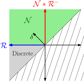
Figure 5: The law of the final maximal point of an N-excursion from Theorem 2.15 depends on the drift vector $\delta=(\delta_{x},\delta_{y})$ from (12). The limit law is either a discrete, normal $\mathcal{N}$, Rayleigh $\mathcal{R}$, or the convolution $\mathcal{N}*\mathcal{R}^{-}$ of a normal and a Rayleigh distribution with negative support. Above we see the drift vector $\delta=(-1/3,1/3)$ for the equidistributed case, i.e., $S(x,y)=\frac{xy}{3}+\frac{y}{3x}+\frac{1}{3xy}$.

Remark 2.16 (Phase transitions of the limit law of the maximal reachable point).

The previous proof shows, that every sector in Figure 5 corresponds to a different dominant singularity from (13). Starting with a drift vector corresponding to the discrete case and continuing in positive direction, we see the following behavior: First, the dominant singularity is of square-root type arsing from $\rho_{1}$; then it coalesces with $\rho_{3}(u)$ creating a different square-root singularity giving a Rayleigh distribution; then it continues as a polar singularity arsing from $\rho_{3}(u)$ giving a normal distribution; which then coalesces with $\rho_{2}(u)$ to form the convolution of a Rayleigh and a normal distribution; finally, it is again a square-root singularity arsing from $\rho_{2}(u)$ giving a normal distribution.

Remark 2.17 (Non-degeneracy of N-meanders).

The restriction $p_{-1,1}\neq 0$ ensures the non-deterministic character of the walks. If $p_{-1,1}=0$ these are classical excursions where the set of reachable points consists of the single end point.

Remark 2.18 (Limit law of lattice paths in the quarter plane with reflecting/absorbing boundaries).

The result of Theorem 2.15 can also be interpreted in terms of two-dimensional lattice paths defined in Figure 3. It gives the limit law of the $y$-coordinate of walks ending on the nonnegative $y$-axis that are confined to the quarter plane and have a reflecting $y$-axis and an absorbing $x$-axis (or, for this step set, absorbing origin).

Let us compare it to the model with an absorbing $y$-axis instead, i.e., the step set at the $y$-axis is always $p_{1}u$. The problem is easier in that case, and we invite the reader to solve this problem as a short exercise in the kernel method. The resulting closed form shows that the limit law follows a binomial distribution independent of the drift. Therefore, it converges in all cases after standardization to a normal distribution.

Next we consider the number of returns to zero of a random N-excursion. We define it as the number of times the set of reachable points is equal to the initial set: $\{0\}$. Let $F(u,t)$ be the bivariate generating function of Dyck N-excursions, where $t$ marks the length and $u$ the number of returns to zero. Every N-excursion can be decomposed into two parts with respect to its last return to zero. The initial part is an N-excursion ending with $\{0\}$ of reachable points given by $D^{+}(0,0,t)$. The second part is an N-excursion with no returns to zero and counted by $\frac{D^{+}(0,1,t)}{D^{+}(0,0,t)}$. Finally, decomposing the initial N-excursions ending in $\{0\}$ into a sequence of minimal paths, in the sense that they have exactly one return to zero, we get

$$F(u,t) =\frac{1}{1-u\left(1-\frac{1}{D^{+}(0,0;t)}\right)}\frac{D^{+}(0,1;t)}{D^{+}(0,0;t)}.$$ (15)

We conclude this section with the limit law of the returns to zero of Dyck N-excursions drawn uniformly at random. In terms of the two-dimensional lattice path defined in Figure 3, this corresponds to the law of the number of visits of the origin of a path ending on the $y$-axis. The law is always discrete; see also Figure 6 for some explicit simulations matching the theoretical results.

Theorem 2.19.

Let $Y_{n}$ be the random variable of the distribution of the number of returns to zero in an N-excursion of length $2n$ drawn uniformly at random:

$$\mathds{P}\left(Y_{n}=k\right) =\frac{[t^{2n}u^{k}]F(u,t)}{[t^{2n}]D^{+}(0,1;t)}.$$

Then, $Y_{n}$ admits a discrete limit distribution of geometric, negative binomial, or mixed type that is given by

$$\mathds{P}\left(Y_{n}=k\right) =\begin{cases}\frac{1}{D^{+}(0,0;1)}\left(1-\frac{1}{D^{+}(0,0;1)}\right)^{k}&\text{ if }0\leq p_{1}\leq p_{-1}<\frac{1}{2},\\ (1-p_{-1})p_{-1}^{k}&\text{ if }0\leq p_{-1}<\frac{1}{2}\text{ and }p_{1}=\frac{1}{2},\\ \frac{1}{2^{k+1}}&\text{ if }0\leq p_{1}<\frac{1}{2}\text{ and }p_{-1}=\frac{1}{2},\\ \frac{k}{2^{k+1}}&\text{ if }p_{1}+p_{-1}=1,\\ \frac{1}{D^{+}(0,0;\rho_{2})}\left(1-\frac{1}{D^{+}(0,0;\rho_{2})}\right)^{k}&\text{ if }0\leq p_{-1}<\frac{1}{2}<p_{1}<1\text{ and }p_{-1}+p_{1}<1,\\ \frac{1+\eta^{k-1}}{2^{k+1}}&\text{ if }0\leq p_{1}<\frac{1}{2}<p_{-1}<1\text{ and }p_{-1}+p_{1}<1,\end{cases}$$

where $\rho_{2}=\frac{1}{4p_{1}(1-p_{1})}$ and $\eta=\frac{p_{-1}(p_{-1}-p_{1})-\sqrt{p_{-1}(1-p_{-1})(1-p_{1}-p_{-1})(p_{-1}-p_{1})}}{p_{-1}(1-p_{1})}\in[0,1]$.

Proof.

Extracting the $k$th coefficient of $u$ in (15) gives

$$\left(1-\frac{1}{D^{+}(0,0;t)}\right)^{k}\frac{D^{+}(0,1;t)}{D^{+}(0,0;t)}.$$

Then, it is straightforward to use singularity analysis [19] to derive the asymptotic expansions. Therefore, we combine the singular expansions of $D^{+}(0,1;t)$ from (11) and of $D^{+}(0,0;t)$ derived from (8) and (9). Note that the cases leading to a negative binomial distribution when $p_{1}+p_{-1}=1$ also follow from [2, Theorem 5]. ∎

(a) Distribution of maximum.

(b) Returns to $0$.

Figure 6: Maximum point reached at the end according to path length (left) and returns to $0$ (right) of Dyck N-excursions (averaged simulation over $10^{5}$ runs).

After this detailed discussion of nondeterministic walks derived from Dyck paths, we turn to the probably next most classical lattice paths: Motzkin paths.

3 Motzkin N-walks

The step set of classical Motzkin paths is $\{-1,0,1\}$. The N-step set of all non-empty subsets is

$$S_{M}=\Big{\{}\{-1\},\{0\},\{1\},\{-1,0\},\{-1,1\},\{0,1\},\{-1,0,1\}\Big{\}},$$

and we call the corresponding N-walks (N-meanders, N-excursions, …) Motzkin N-walks (Motzkin N-meanders, Motzkin N-excursions, …). Note that we will perform the subsequent analysis only in the unweighted case, however, as shown in the previous section on Dyck N-walks, it is straightforward to generalize the results to the weighted case.

3.1 Motzkin N-walks and N-bridges

As for Dyck N-walks, we start with a description of the reachable points of Motzkin N-walks. Here, we need to distinguish two cases.

Definition 3.1 (Types of reachable points).

A Motzkin N-walk $w$ is

• of type $\operatorname{{I}}$ if $\operatorname{reach}(w)=\left\{\min(w)+i~{}:~{}i=0,1,\dots,\|w\|\right\}$ and $\|w\|\geq 1$.

• of type $\operatorname{{II}}$ if $\operatorname{reach}(w)=\left\{\min(w)+2i~{}:~{}i=0,1,\dots,\frac{\|w\|}{2}\right\}$,

In other words, the sets of reachable points are either $1$- or $2$-periodic finite subsets of integers. The condition $\|w\|\geq 1$ guarantees that the types are disjoint. For Dyck N-walks we did not need to distinguish different types, as they where always of type $\operatorname{{II}}$. Now, the following proposition will explain how these two types suffice to characterize the structure of Motzkin N-walks.

Proposition 3.2.

A Motzkin N-walk $w$ is of type $\operatorname{{II}}$ if and only if it is constructed only from the N-steps $\{-1\}$, $\{0\}$, $\{1\}$, and $\{-1,1\}$. Otherwise, it is of type $\operatorname{{I}}$; see Figure 7.

Proof.

We use induction on the number of N-steps. If the Motzkin N-walk is empty, its set of reachable points is $\{0\}$, which is of type $\operatorname{{II}}$ by definition. Now consider a Motzkin N-walk $w$ of reachable points $\bm{r}$, a Motzkin N-step $\bm{s}$, and the set of reachable points of $w\cdot\bm{s}$, given by $\bm{r}+\bm{s}$. Let us assume the proposition holds for $w$ and prove it for $w\cdot\bm{s}$.

If $\bm{s}$ has size $1$, like $\{-1\}$, $\{0\}$ or $\{1\}$, $\bm{r}+\bm{s}$ is just a translation of $\bm{r}$, so the type is unchanged.

If $\bm{r}$ is of type $\operatorname{{I}}$, it is an integer interval of size $\ell\geq 2$, so there exists $m\in\mathds{Z}$ such that $\bm{r}=[m,m+\ell]$. Then for any Motzkin N-step $\bm{s}$, $\bm{r}+\bm{s}$ is also an integer interval, of size $\ell+\max(\bm{s})-\min(\bm{s})$.

If $\bm{r}$ is of type $\operatorname{{II}}$ and $\bm{s}=\{-1,1\}$, then we saw in Lemma 2.1 that $\bm{r}+\bm{s}$ has type $\operatorname{{II}}$. The last case is when $\bm{r}$ has type $\operatorname{{II}}$, say $\bm{r}=\{m,m+2,\ldots,m+2\ell\}$, and $\bm{s}$ is equal to $\{-1,0\}$, $\{0,1\}$, or $\{-1,0,1\}$. The value of $\bm{r}+\bm{s}$, in each case, is $[m-1,m+2\ell]$, $[m,m+2\ell+1]$ or $[m-1,m+2\ell+1]$. It is always an interval of length at least $2$, so it is of type $\operatorname{{I}}$. ∎

Figure 7: The automaton representing the structure of reachable points of Motzkin N-walks.

The set of Motzkin N-walks of type $\operatorname{{I}}$ (resp. $\operatorname{{II}}$) is denoted by $M_{\operatorname{{I}}}$ (resp. $M_{\operatorname{{II}}}$), and their generating functions are defined as

$$M_{\operatorname{{I}}}(x,y;t) =\sum_{w\in M_{\operatorname{{I}}}}x^{\min(w)}y^{\max(w)}t^{|w|},$$

$$M_{\operatorname{{II}}}(x,y;t) =\sum_{w\in M_{\operatorname{{II}}}}x^{\min(w)}y^{\max(w)}t^{|w|}.$$

The generating function for all Motzkin N-walks is defined as $M(x,y;t)=M_{\operatorname{{I}}}(x,y;t)+M_{\operatorname{{II}}}(x,y;t)$.

Theorem 3.3.

The generating functions of Motzkin N-walks of type $\operatorname{{I}}$ and $\operatorname{{II}}$, as well as for all Motzkin N-walks are rational.

Proof.

This result is a direct consequence of the analysis of the interactions of types and N-steps in the proof of Proposition 3.2; see also Figure 7. Translating the change in the minimal and maximal reachable points for each step into polynomials, we directly get

$$M_{\operatorname{{II}}}(x,y;t) =1+t\left(\frac{1}{xy}+1+xy+\frac{y}{x}\right)M_{\operatorname{{II}}}(x,y;t),$$

$$M_{\operatorname{{I}}}(x,y;t) =t\left(\frac{1}{x}+y+\frac{y}{x}\right)M_{\operatorname{{II}}}(x,y;t)+t\left(\frac{1}{xy}+1+xy+\frac{1}{x}+y+2\frac{y}{x}\right)M_{\operatorname{{I}}}(x,y;t).$$

Hence, both generating function are rational with explicit solutions, and therefore also $M(x,y,t)$. Alternatively, note that by Remark 2.6 the closed form of $M(x,y,t)$ is given by (7). ∎

Theorem 3.4.

The generating function of Motzkin N-bridges is algebraic.

Proof.

An N-bridge $w$ of type $\operatorname{{II}}$ is an $M_{\operatorname{{II}}}$ N-walk that satisfies $\min(w)\leq 0$, $\max(w)\geq 0$, and $\min(w)$ even. An N-bridge $w$ of type $\operatorname{{I}}$ is an $M_{\operatorname{{I}}}$ N-walk that satisfies $\min(w)\leq 0$ and $\max(w)\geq 0$. Thus, the generating function of Motzkin N-bridges is equal to

$$[x^{\leq 0}y^{\geq 0}]\left(\frac{M_{\operatorname{{II}}}(x,y;t)+M_{\operatorname{{II}}}(-x,y;t)}{2}+M_{\operatorname{{I}}}(x,y;t)\right).$$

Since the generating functions of $M_{\operatorname{{I}}}$ and $M_{\operatorname{{II}}}$ are rational, the generating function of N-bridges is D-finite; see [11, Proposition 1] and [26]. Yet the generating function is even algebraic, which can be proved similarly to as done in the proof of Theorem 2.4. The main observation is that, as in (4), the simultaneous extraction of nonnegative and nonpositive parts can be rewritten into two single extractions from a rational generating function, which are therefore both algebraic. ∎

Remark 3.5 (Closed forms and asymptotics).

Using the computer algebra system Maple, we computed closed forms, which we however do not state here explicitly due to their size; full details are given in the accompanying Maple worksheet. From these closed forms it is then straightforward to compute the asymptotics given in Table 1 using singularity analysis. This proves that the proportion of Motzkin N-bridges among all Motzkin N-walks of length $n$ is equal to

$$1-\sqrt{\frac{3}{\pi}}\frac{(6/7)^{n}}{\sqrt{n}}+\mathcal{O}\left(\frac{(6/7)^{n}}{n^{3/2}}\right).$$

Hence, nearly all Motzkin N-walks are N-bridges.

We now turn to the analysis of Motzkin N-meanders and N-excursions.

3.2 Motzkin N-meanders and N-excursions

The key to enumerate N-meanders is to understand their reachable points. The difference to N-walks is that N-meanders cannot go below the $x$-axis. Recall that if an N-step would go below the $x$-axis, only the steps staying weakly above it are appended. The following proposition shows that the two types from Definition 3.1 suffice to characterize the reachable points. However, the types interact with the N-steps differently than before.

Figure 8: The automaton representing the structure of reachable points of Motzkin N-meanders. Here, “$\max$” refers to the maximal reachable point of the N-meander.

Proposition 3.6.

Let $w$ be a Motzkin N-meander and $\bm{s}\in S_{M}$.

• If $w$ has type $\operatorname{{II}}$, then $w\cdot\bm{s}$ has type $\operatorname{{II}}$ if $\bm{s}\in\{\{-1\},\{0\},\{1\},\{-1,1\}\}$, type $\operatorname{{I}}$ otherwise.

• If $w$ has type $\operatorname{{I}}$ and $\max^{+}(w)>1$ then $w\cdot\bm{s}$ has type $\operatorname{{I}}$ for any $\bm{s}$.

• If $w$ has type $\operatorname{{I}}$ and $\max^{+}(w)=1$ (i.e., the reachable points are $\{0,1\}$) then $w\cdot\bm{s}$ has type $\operatorname{{II}}$ if $\bm{s}=\{-1\}$, and type $\operatorname{{I}}$ otherwise; see Figure 8.

Proof.

The first two cases follow directly from Proposition 3.2. The last case is different, due to the interaction with the boundary, reducing the integer interval to a singleton. ∎

Let $M_{\operatorname{{I}}}^{+}$ and $M_{\operatorname{{II}}}^{+}$ denote the set of Motzkin N-meanders of type $\operatorname{{I}}$ and $\operatorname{{II}}$, respectively. Their generating functions are defined as

$$M_{\operatorname{{I}}}^{+}(x,y;t) =\sum_{w\in M_{\operatorname{{I}}}^{+}}x^{\min^{+}(w)}y^{\max^{+}(w)}t^{|w|},$$

$$M_{\operatorname{{II}}}^{+}(x,y;t) =\sum_{w\in M_{\operatorname{{II}}}^{+}}x^{\min^{+}(w)}y^{\max^{+}(w)}t^{|w|}.$$

The generating function for all Motzkin N-meanders is defined as $M^{+}(x,y;t)=M_{\operatorname{{I}}}^{+}(x,y;t)+M_{\operatorname{{II}}}^{+}(x,y;t)$. Now, Proposition 3.6 allows us now to characterize Motzkin N-meanders and N-excursions.

Theorem 3.7.

The generating functions $M_{\operatorname{{I}}}^{+}(x,y;t)$ and $M_{\operatorname{{II}}}^{+}(x,y;t)$ of Motzkin N-meanders of type $\operatorname{{I}}$ and $\operatorname{{II}}$, respectively, are algebraic. In particular, Motzkin N-meanders $M^{+}(x,y;t)$ and N-excursions $M_{\operatorname{{I}}}^{+}(0,y;t)$, $M_{\operatorname{{II}}}^{+}(0,y;t)$ are algebraic.

Proof.

Observe that $M_{\operatorname{{I}}}^{+}(x,y;t)$ is divisible by $y$, as N-meanders of type $\operatorname{{I}}$ have maximal reachable point at least $1$. Let $\bm{M^{+}}(x,y;t)$ denote the column vector $(M_{\operatorname{{II}}}^{+}(x,y;t),y^{-1}M_{\operatorname{{I}}}^{+}(x,y;t))^{T}$. An N-meander is either empty, and associated with type $\operatorname{{II}}$, or an N-meander to which we append an N-step. This translates into a step-by-step construction analogous to the proof of Proposition 2.5, yet now for two types and with interactions between them. Again we distinguish three cases: general case ($\min^{+}(w)>0$), boundary case ($\min^{+}(w)=0$) but non-minimal maximum ($\max^{+}(w)>0$ for type $\operatorname{{II}}$ or $\max^{+}(w)>1$ for type $\operatorname{{I}}$), and boundary case ($\min^{+}(w)=0$) with minimal maximum ($\max^{+}(w)=0$ for type $\operatorname{{II}}$ or $\max^{+}(w)=1$ for type $\operatorname{{I}}$). We get the following system of equations characterizing the generating functions of the vector $\bm{M^{+}}(x,y;t)$:

$$\bm{M^{+}}(x,y;t) =\bm{e_{1}}+t\Big{(}A(x,y)(\bm{M^{+}}(x,y;t)-\bm{M^{+}}(0,y;t))$$

$$\quad+B(x,y)(\bm{M^{+}}(0,y;t)-\bm{M^{+}}(0,0;t))$$

$$\quad+C(x,y)\bm{M^{+}}(0,0;t)\Big{)},$$

where $\bm{e_{1}}$ is the column vector $(1,0)$, and $A(x,y)$, $B(x,y)$, $C(x,y)$ are two-by-two matrices with Laurent polynomials in $x$ and $y$ given in Figure 9. These matrices model the interactions of the two types with the N-steps from Proposition 3.6 and the change in the minima and maxima of the reachable points.

$$A(x,y) ={\small\begin{pmatrix}x^{-1}y^{-1}+1+xy+x^{-1}y&0\\ x^{-1}y^{-1}+1+x^{-1}&x^{-1}y^{-1}+1+xy+x^{-1}+y+2x^{-1}y\end{pmatrix}},$$

$$B(x,y) ={\small\begin{pmatrix}xy^{-1}+1+2xy&0\\ y^{-1}+2&y^{-1}+2+xy+3y\end{pmatrix}},\qquad C(x,y)={\small\begin{pmatrix}2+2xy&1\\ 2&xy+2+3y\end{pmatrix}}.$$

Figure 9: Type transition matrices involved in the proof of Theorem 3.7.

Next, we rearrange this equation into

$$\begin{aligned} \left(\operatorname{Id}-tA(x,y)\right)\bm{M^{+}}(x,y;t)&=\bm{e_{1}}-t\left(A(x,y)-B(x,y)\right)\bm{M^{+}}(0,y;t)\\ &\quad-t\left(B(x,y)-C(x,y)\right)\bm{M^{+}}(0,0;t).\end{aligned}$$ (16)

On the left hand side, we identify a factorization involving the explicit factor $K(x,y,t)=\operatorname{Id}-tA(x,y)$. If this system would consist of only a single equation, we could apply the classical kernel method; see, e.g., [2]. However, for this system we need to generalize this approach to matrix equations; see [1] for similar generalizations. Our idea is to choose specific values of $x$, such that $K(x,y,t)$ becomes singular, and then left-multiply by an element from its kernel to deduce a new identity. Due to the triangular nature of $A(x,y)$, the matrix $K(x,y,t)$ is singular when one of the following two equations is satisfied.

$$1-tA_{0,0}(x,y) =0,$$

$$1-tA_{1,1}(x,y) =0.$$

This gives two candidates $X_{1}(y,t)$ and $X_{2}(y,t)$ with the following closed forms:

$$X_{1}(y,t) =\frac{1-t-\sqrt{1-4t^{2}y^{2}-3t^{2}-2t}}{2ty},$$

$$X_{2}(y,t) =\frac{1-t(y+1)-\sqrt{1-7t^{2}y^{2}-2t^{2}y-3t^{2}-2ty-2t}}{2ty}.$$

Note that the final generating functions are power series in $t$, hence we need to choose these two branches. We then define the row vectors

$$\bm{u_{1}} =(1,0),$$

$$\bm{u_{2}}(y,t) =\left(tA_{1,0}(X_{2}(y,t),y),1-tA_{0,0}(X_{2}(y,t),y)\right),$$

so that the left-hand side of Equation (16) vanishes when evaluated at $x=X_{1}(y,t)$ and left-multiplied by $\bm{u_{1}}$, and also when evaluated at $x=X_{2}(y,t)$ and left-multiplied by $\bm{u_{2}}(y,t)$. Combining the corresponding two right-hand sides, we obtain a new two-by-two system of linear equations

$$tD(y,t)\bm{M^{+}}(0,y;t)=\bm{f}(y,t)-E(y,t)\bm{M^{+}}(0,0;t),$$ (17)

where the vector $\bm{f}(y,t)$ of size $2$ has its first element equal to $1$, and its second element equal to

$$\frac{{\left(ty+t-\sqrt{-7\,t^{2}y^{2}-3\,t^{2}-2\,{\left(t^{2}+t\right)}y-2\,t+1}+1\right)}t}{1-ty-t-\sqrt{-7\,t^{2}y^{2}-3\,t^{2}-2\,{\left(t^{2}+t\right)}y-2\,t+1}},$$

and the two-by-two matrices $D(y,t)$ and $E(y,t)$ are two large to be shown here. Again, the matrix $D(y,t)$ is upper-triangular, and we repeat the process from above now with respect to the variable $y$. Now, $D(y,t)$ becomes singular, when $y$ is evaluated at one of the following branches (again we choose the power series solutions in $t$):

$$Y_{1}(t) =\frac{t-1+\sqrt{1-2t-7t^{2}}}{4t},$$

$$Y_{2}(t) =\frac{1-2t-\sqrt{1-4t-12t^{2}}}{8t}.$$

Next, we deduce the following two row vectors as elements of the respective kernels:

$$\bm{v_{1}} =(1,0),$$

$$\bm{v_{2}}(t) =(-D_{1,0}(Y_{2}(t),t),D_{0,0}(Y_{2}(t),t)),$$

Hence, the left-hand side of Equation (17) vanishes when evaluated at $y=Y_{1}(t)$ and left-multiplied by $\bm{v_{1}}$, and also when evaluated at $y=Y_{2}(t)$ and left-multiplied by $\bm{v_{2}}(t)$. Combining the corresponding two new equations we get

$$\bm{h}(t)=tF(t)\bm{M^{+}}(0,0;t),$$

where the column vector $h(t)$ and the matrix $F(t)$ are too large to be shown here. The matrix $F(t)$ is invertible, so the generating function of Motzkin N-meanders with maximum reachable point $0$, i.e., N-excursions ending in $\{0\}$, is equal to

$$\bm{M^{+}}(0,0;t)=\frac{1}{t}F(t)^{-1}\bm{h}(t).$$

Then we substitute this expression into Equation (17) to express the generating function of Motzkin N-meanders with minimum reachable point $0$, i.e., N-excursions, as

$$\bm{M^{+}}(0,y;t)=\frac{1}{t}D(y,t)^{-1}(\bm{f}(y,t)-E(y,t)\bm{M^{+}}(0,0;t)).$$

Finally, we substitute this expression into Equation (16) to express the generating function of Motzkin N-meanders as

$$\bm{M^{+}}(x,y;t) =\left(\operatorname{Id}-tA(x,y)\right)^{-1}(\bm{e_{1}}-t\left(A(x,y)-B(x,y)\right)\bm{M^{+}}(0,y;t)$$

$$\quad-t\left(B(x,y)-C(x,y)\right)\bm{M^{+}}(0,0;t)).$$

The generating function of N-meanders and N-excursions are then, respectively, $M_{\operatorname{{I}}}^{+}(x,y;t)+M_{\operatorname{{II}}}^{+}(x,y;t)$ and $M_{\operatorname{{I}}}^{+}(0,y;t)+M_{\operatorname{{II}}}^{+}(0,y;t)$. ∎

As before we can use a computer algebra system to compute explicit results. In Section A we considered all possible combination of weights $p_{s}\in\{0,1\}$ for $s\in S_{M}$ for N-excursions and N-meanders and found several connections with known sequences in the OEIS, yet most of them are not. For example, when all $p_{i}$’s are equal to $1$ neither the sequences of N-meanders nor N-excursions are in the OEIS. In this case, the generating function of N-meanders $M^{+}(1,1;t)$ is algebraic of degree $2$ and given by

$$M^{+}(1,1;t) =\frac{10t-1+\sqrt{(1+2t)(1-6t)}}{8t(1-7t)}.$$

The total number of N-meanders is asymptotically equal to

$$\frac{3}{4}7^{n}+\frac{3\sqrt{3}}{2\sqrt{\pi}}\frac{6^{n}}{\sqrt{n^{3}}}+\mathcal{O}\left(\frac{6^{n}}{n^{5/2}}\right).$$

The generating function $E=M^{+}(0,1;t)$ of N-excursions is algebraic of degree $4$ and satisfies

$$256\,{t}^{5}\left(2\,t+1\right)^{2}\left(7\,t-1\right)^{2}\left(4\,t-1\right)^{2}{E}^{4}$$

$$+16\,{t}^{2}\left(2\,t+1\right)\left(7\,t-1\right)\left(4\,t-1\right)\left(564\,{t}^{5}-192\,{t}^{4}-85\,{t}^{3}+69\,{t}^{2}-15\,t+1\right){E}^{3}$$

$$+\left(197264\,{t}^{9}-44448\,{t}^{8}-68144\,{t}^{7}+36720\,{t}^{6}-864\,{t}^{5}-4624\,{t}^{4}+1742\,{t}^{3}-303\,{t}^{2}+27\,t-1\right){E}^{2}$$

$$+\left(36000\,{t}^{8}-12220\,{t}^{7}-14436\,{t}^{6}+8901\,{t}^{5}+121\,{t}^{4}-1256\,{t}^{3}+375\,{t}^{2}-45\,t+2\right)E$$

$$+4288\,{t}^{7}-456\,{t}^{6}-1901\,{t}^{5}+591\,{t}^{4}+170\,{t}^{3}-108\,{t}^{2}+18\,t-1=0.$$

The total number of Motzkin N-excursions is asymptotically equivalent to

$$\frac{9}{16}7^{n}-\gamma\frac{6^{n}}{\sqrt{\pi n^{3}}}+\mathcal{O}\left(\frac{6^{n}}{n^{5/2}}\right),\quad$$

where $\gamma\approx 0.6183$ is the positive real solution of $1024\gamma^{4}-8019\gamma^{2}+2916=0$. This means that for large $n$ approximately $75\%$ of all N-walks are N-meanders and $56.25\%$ of all N-walks are N-excursions.

3.3 Bijections with two-dimensional lattice paths

Any N-step set can be interpreted as a two-dimensional lattice path problem. The minimum reachable point is mapped to the $x$-coordinate and the maximum reachable point to the $y$-coordinate: We define the mapping $\varphi$ from N-steps to two-dimensional steps as

$$\varphi(s)=\left(\min(s),\max(s)\right).$$

This generalizes the previously discussed mapping (3). For Motzkin N-steps $S_{M}$ this gives the following mapping to nearest neighbor steps:

$$\{-1\} \mapsto(-1,-1), \{0,1\} \mapsto(0,1), \{-1,1\} \mapsto(-1,1)_{1},$$

$$\{0\} \mapsto(0,0), \{-1,0\} \mapsto(-1,0), \{-1,0,1\} \mapsto(-1,1)_{2},$$

$$\{1\} \mapsto(1,1).$$

Note that the step $(-1,1)$ comes in two colors, depending on whether it corresponds to $\{-1,1\}$ or $\{-1,0,1\}$. We denote the two colors by $(-1,1)_{1}$ and $(-1,1)_{2}$. Moreover, by construction the steps $(1,0)$, $(1,-1)$, and $(0,-1)$ will never be used. This played a crucial role in proving the algebraicity of N-bridges in Theorems 2.4 and 3.4 as it led to Equation (4). In the following section, we will show that this fact holds for arbitrary finite N-step sets, and also allows to prove the algebraicity of general N-bridges.

Now we use $\varphi$ to give bijections between different families of Motzkin N-walks and two-dimensional walks. In general the steps above are used, just on the axes we might need to modify the steps; compare with Figure 3.

1. N-walks are in bijection with unconstrained two-dimensional walks.

2. N-bridges are in bijection with two-dimensional walks ending in the second quadrant, where if only steps $\{(-1,1),(0,0),(1,1),(-1,1)_{1}\}$ are used it has to be of even length.

3. N-meanders are in bijection with two-dimensional walks confined to the first quadrant, where the positive $y$-axis and the origin use different steps that depend on the possible types.

4. N-excursions are in bijection with two-dimensional walks associated with N-meanders that end on the $y$-axis.

4 N-bridges with general N-steps

We have already seen in (7) that the generating function of N-walks is always rational. In this section we treat the generating function of N-bridges for arbitrary finite N-step set. The following main result generalizes Theorems 2.4 and 3.4.

Theorem 4.1.

For any finite N-step set $S$, the generating function $B(x,y;t)$ of N-bridges with respect to length, minimal, and maximal reachable point is algebraic.

A method for computing this generating function is provided by the proof, in Subsection 4.2. In order to establish this result, we first establish the required algebraic setting.

4.1 Sumset monoid

This subsection contains the algebraic definitions needed to describe sets of reachable points of N-walks on a given N-step set.

Finite integer sets.

We consider the set $\mathcal{F}$ containing all finite sets of integers

$$\mathcal{F}=\{\bm{s}\mid\bm{s}\subset\mathds{Z},\ |\bm{s}|<\infty\}.$$

They will represent N-steps as well as sets of reachable points.

Sum.

It is equipped with a sum, known as the sumset or Minkowski sum, and defined by

$$\bm{s}+\bm{t}=\{a+b\mid a\in\bm{s},\ b\in\bm{t}\}.$$

This is a central operation in additive combinatorics [32]. Together, $\mathcal{F}$ and the sumset operation form a commutative monoid with neutral element $\{0\}$. Observe that for any $\bm{s}\in\mathcal{F}$, we have $\bm{s}+\emptyset=\emptyset$. Furthermore, shifting a set $\bm{s}$ by $c\in\mathds{Z}$ corresponds to a sumset with the set $\{c\}$

$$\bm{s}+\{c\}=\{a+c\mid a\in\bm{s}\}.$$

The link with N-walks is that the set of reachable points $\bm{r}$ of any N-walk $w=\bm{s}_{1}\cdots\bm{s}_{n}$ is the sumset of its N-steps: $\bm{r}=\bm{s}_{1}+\cdots+\bm{s}_{n}$.

Product.

Given a nonnegative integer $n$ and $\bm{s}\in\mathcal{F}$, we define $n\times\bm{s}$ as the $n$-fold sumset of $\bm{s}$ with itself

$$n\times\bm{s}=\bm{s}+\cdots+\bm{s}=\{a_{1}+\cdots+a_{n}\mid a_{i}\in\bm{s}\}.$$

For example, we have

$$n\times\{0,m\}=\{k\,m\mid 0\leq k\leq n\}$$

and $0\times\bm{s}=\{0\}$ by convention.

Norm.

The norm of any $\bm{s}\in\mathcal{F}$ is defined as

$$\|\bm{s}\|=\begin{cases}0&\text{if }\bm{s}=\emptyset,\\ \max(\bm{s})-\min(\bm{s})&\text{otherwise.}\end{cases}$$

Bottom pruning.

Let $\bm{s},\bm{t}\in\mathcal{F}$ be two sets of integers. Then bottom pruning is defined as

$$\bm{s}\smash{\mskip 4.0mu\raise 5.8125pt\hbox to0.0pt{\begin{turn}{180.0}$\hat{\phantom{-}}$\end{turn}\hss}-}\mskip 4.0mu{\vphantom{\widehat{-}}}\bm{t}=\begin{cases}\emptyset&\text{if }\bm{s}=\emptyset,\\ \bm{s}\setminus(\{\min(\bm{s})\}+\bm{t})&\text{otherwise.}\end{cases}$$

It corresponds to shifting $\bm{t}$ to the bottom of $\bm{s}$, and then removing the corresponding elements from $\bm{s}$. In other words, $\bm{t}$ accounts for the elements relative to $\min(\bm{s})$. Note that negative elements in $\bm{t}$ will always lie outside the range after shifting. For example, removing the smallest element of $\bm{s}$ corresponds to removing $\{0\}$, and

$$\{3,4,6,7,8\}\smash{\mskip 4.0mu\raise 5.8125pt\hbox to0.0pt{\begin{turn}{180.0}$\hat{\phantom{-}}$\end{turn}\hss}-}\mskip 4.0mu{\vphantom{\widehat{-}}}\{-2,1,3,5\}=\{3,4,6,7,8\}\setminus\{1,4,6,8\}=\{3,7\}.$$

Top pruning.

Let $\bm{s},\bm{t}\in\mathcal{F}$ be two sets of integers. Then top pruning is defined as

$$\bm{s}\smash{\mskip 4.0mu\raise-2.15277pt\hbox to0.0pt{$\hat{\phantom{-}}$\hss}-}\mskip 4.0mu{\vphantom{\widehat{-}}}\bm{t}=\begin{cases}\emptyset&\text{if }\bm{s}=\emptyset,\\ \bm{s}\setminus(\{\max(\bm{s})\}-\bm{t})&\text{otherwise.}\end{cases}$$

Top pruning corresponds to removing from the top, where $\bm{t}$ accounts for the elements relative to $\max(\bm{s})$ from top to bottom. Again, negative elements in $\bm{t}$ will lie outside the range after shifting. For example, removing the largest element of $\bm{s}$ corresponds to a top pruning by $\{0\}$, and

$$\{0,1,2,3,4\}\smash{\mskip 4.0mu\raise-2.15277pt\hbox to0.0pt{$\hat{\phantom{-}}$\hss}-}\mskip 4.0mu{\vphantom{\widehat{-}}}\{1,2\}=\{0,1,4\}.$$

Compare the previous example to the bottom pruning

$$\{0,1,2,3,4\}\smash{\mskip 4.0mu\raise 5.8125pt\hbox to0.0pt{\begin{turn}{180.0}$\hat{\phantom{-}}$\end{turn}\hss}-}\mskip 4.0mu{\vphantom{\widehat{-}}}\{1,2\}=\{0,3,4\}.$$

Equivalence.

Two integer sets $\bm{s},\bm{t}\in\mathcal{F}$ are equivalent, denoted by $\bm{s}\sim\bm{t}$, if there exists an integer $m$ such that $\bm{s}=\bm{t}+\{m\}$. In other words, one can be obtained from the other by a shift.

Conjugate.

The conjugate of an element of $\bm{s}\in\mathcal{F}$ is defined as

$$\overline{\bm{s}}=\{\min(\bm{s})+\max(\bm{s})-a\mid a\in\bm{s}\}.$$

For example, the conjugate of $\{1,3,4\}$ is $\{1,2,4\}$. Furthermore, bottom and top pruning are linked by conjugation

$$\overline{\bm{s}}\smash{\mskip 4.0mu\raise 5.8125pt\hbox to0.0pt{\begin{turn}{180.0}$\hat{\phantom{-}}$\end{turn}\hss}-}\mskip 4.0mu{\vphantom{\widehat{-}}}\bm{t}\sim\overline{\bm{s}\smash{\mskip 4.0mu\raise-2.15277pt\hbox to0.0pt{$\hat{\phantom{-}}$\hss}-}\mskip 4.0mu{\vphantom{\widehat{-}}}\bm{t}}.$$

Type.

For two nonnegative integers $n$, $k$ and $\bm{a},\bm{b},\bm{c}\in\mathcal{F}$, we define $\operatorname{type}(n,k,\bm{a},\bm{b},\bm{c})$ as the following subset of $\mathcal{F}$:

$$\operatorname{type}(n,k,\bm{a},\bm{b},\bm{c})=\left\{j\times\{0,n\}+\bm{b}\smash{\mskip 4.0mu\raise 5.8125pt\hbox to0.0pt{\begin{turn}{180.0}$\hat{\phantom{-}}$\end{turn}\hss}-}\mskip 4.0mu{\vphantom{\widehat{-}}}\bm{a}\smash{\mskip 4.0mu\raise-2.15277pt\hbox to0.0pt{$\hat{\phantom{-}}$\hss}-}\mskip 4.0mu{\vphantom{\widehat{-}}}\bm{c}+\{m\}\mid m\in\mathds{Z},\ j\in\mathds{Z}_{\geq k}\right\}.$$

For example,

$$\operatorname{type}(3,1,\emptyset,\{0,1\},\{1,2,3\})=\left\{\{0,4\},\{0,1,3,7\},\{0,1,3,4,6,10\},\{0,1,3,4,6,7,9,13\},\dots\right\}.$$

Provided $n\geq 1$ and $\bm{b}\neq\emptyset$, $\operatorname{type}(n,k,\bm{a},\bm{b},\bm{c})$ contains elements of arbitrarily large norm. However, the key property is that each $\bm{t}\in\operatorname{type}(n,k,\bm{a},\bm{b},\bm{c})$ is uniquely characterized by $\min(\bm{t})$ and $\max(\bm{t})$. We will prove in Lemma 4.2 that there are finitely many possible types for the reachable points of an N-walk on a given N-step set. In our generating functions, we will keep track of the minimal and maximal reachable points, as well as the type of the reachable points. This information will be enough to reconstruct the complete set of reachable points. Below are a few examples of relations between types:

$$\operatorname{type}(0,k,\bm{a},\bm{b},\bm{c}) =\{\bm{b}\smash{\mskip 4.0mu\raise 5.8125pt\hbox to0.0pt{\begin{turn}{180.0}$\hat{\phantom{-}}$\end{turn}\hss}-}\mskip 4.0mu{\vphantom{\widehat{-}}}\bm{a}\smash{\mskip 4.0mu\raise-2.15277pt\hbox to0.0pt{$\hat{\phantom{-}}$\hss}-}\mskip 4.0mu{\vphantom{\widehat{-}}}\bm{c}+\{m\}\mid m\in\mathds{Z}\},$$

$$\operatorname{type}(n,k,\bm{a},\emptyset,\bm{c}) =\{\emptyset\},$$

$$\operatorname{type}(1,0,\emptyset,\{0\},\emptyset) =\{[u,v]\mid v\geq u\},$$

$$\operatorname{type}(n,k,\bm{a},\bm{b}+\{m\},\bm{c}) =\operatorname{type}(n,k,\bm{a},\bm{b},\bm{c}),$$

$$\operatorname{type}(n,k,\bm{a},\bm{b},\bm{c}) =\{\bm{s}\smash{\mskip 4.0mu\raise 5.8125pt\hbox to0.0pt{\begin{turn}{180.0}$\hat{\phantom{-}}$\end{turn}\hss}-}\mskip 4.0mu{\vphantom{\widehat{-}}}\bm{a}\smash{\mskip 4.0mu\raise-2.15277pt\hbox to0.0pt{$\hat{\phantom{-}}$\hss}-}\mskip 4.0mu{\vphantom{\widehat{-}}}\bm{c}\mid\bm{s}\in\operatorname{type}(n,k,\emptyset,\bm{b},\emptyset)\}.$$

Proper type.

A type $(n,k,\bm{a},\bm{b},\bm{c})$ is proper if either

• $n=0$, then $k=0$, $\bm{a}=\bm{c}=\emptyset$ and $\min(\bm{b})=0$, or

• $n>0$, then $\min(\bm{a})\geq 0$, $\min(\bm{c})\geq 0$, $\min(\bm{b})=0$, $\bm{b}\subset[0,n-1]$, and $kn>\max(\bm{a})+\max(\bm{c})$.

The condition on $\bm{b}$ guarantees that in the sumset of $j\times\{0,n\}$ and $\bm{b}$ there are no overlaps. Therefore, all $\bm{s}$ in a proper type are, except for the beginning and the end, constructed using a periodic repetition of a pattern defined by $\bm{b}$ of size $n$.

Since for any $m\in\mathds{Z}$ and type $(n,k,\bm{a},\bm{b},\bm{c})$, we have

$$\operatorname{type}(n,k,\bm{a},\bm{b},\bm{c})=\operatorname{type}(n,k,\bm{a}\cap\mathds{Z}_{\geq 0},\bm{b}+\{m\},\bm{c}\cap\mathds{Z}_{\geq 0}),$$

and

$$\operatorname{type}(0,k,\bm{a},\bm{b},\bm{c})=\operatorname{type}(0,0,\emptyset,\bm{b}\smash{\mskip 4.0mu\raise 5.8125pt\hbox to0.0pt{\begin{turn}{180.0}$\hat{\phantom{-}}$\end{turn}\hss}-}\mskip 4.0mu{\vphantom{\widehat{-}}}\bm{a}\smash{\mskip 4.0mu\raise-2.15277pt\hbox to0.0pt{$\hat{\phantom{-}}$\hss}-}\mskip 4.0mu{\vphantom{\widehat{-}}}\bm{c},\emptyset),$$

any type with $n=0$ is equal to a proper type, and we will prove in Lemma 4.6 that for any type $(n,k,\bm{a},\bm{b},\bm{c})$ with $n>0$, there exists $k^{\prime}$ large enough such that the type $(n,k^{\prime},\bm{a},\bm{b},\bm{c})$ is equal to a proper type.

4.2 Automaton for N-bridges

For N-walks and in particular N-bridges, we will show that finitely many types suffice to capture all possible sets of reachable points (of which in general, however, infinitely many will exist).

Proposition 4.2.

For any finite subset $S\subset\mathcal{F}$, there is a finite set of types $(n_{i},k_{i},\bm{a}_{i},\bm{b}_{i},\bm{c}_{i})_{1\leq i\leq k}$ such that any element generated by $(S,+)$ belongs to $\operatorname{type}(n_{i},k_{i},\bm{a}_{i},\bm{b}_{i},\bm{c}_{i})$ for some $1\leq i\leq k$.

The last proposition is almost enough to prove that general N-bridges have algebraic generating functions. In fact, we rely on the following, more effective, generalization.

Proposition 4.3.

For any finite subset $S\subset\mathcal{F}$ of N-steps, there is a finite automaton $\mathcal{A}$ on the alphabet $S$ where each state corresponds to a proper type, such that for any N-walk $w=(\bm{s}_{1},\ldots,\bm{s}_{m})\in S^{m}$, the sumset $\bm{s}_{1}+\cdots+\bm{s}_{m}$ belongs to the type corresponding to the state that $\mathcal{A}$ reaches after reading $w$. Furthermore, if loops are removed, the directed graph underlying this automaton is acyclic.

Before proving this proposition, we show how it implies the proof of the main result of this section, Theorem 4.1, showing that for any finite N-step set $S$, the generating function of N-bridges is algebraic.

Proof of Theorem 4.1.

We start with the automaton from Proposition 4.3. By construction, each N-walk, read step-by-step, corresponds to a walk on this automaton such that the current state corresponds to the current type of the reachable points. Now, we associate to each state $q$ a generating function

$$F_{q}(x,y;t)=\sum_{n,i,j\geq 0}f^{(q)}_{i,j,n}x^{i}y^{j}t^{n},$$

where $f^{(q)}_{i,j,n}$ is the number of N-walks of length $n$ whose reachable points have type associated to $q$, minimum $i$, and maximum $j$. As in the previous proofs of Theorems 2.4 and 3.4 for the Dyck and Motzkin cases, it is now easy to build a characterizing system of equations for $F_{q}(x,y;t)$. This system is finite and therefore each generating function is rational.

It remains to extract N-bridges, i.e., N-walks $w$ such that $0\in\operatorname{reach}(w)$. We can do this now for each type individually. For all types, it is necessary that $i\leq 0$ and $j\geq 0$. In terms of generating functions, this translates to

$$\tilde{B}_{q}(x,y;t):=F_{q}(x,y;t)-[x^{>0}]F_{q}(x,y;t)-[y^{<0}]F_{q}(x,y;t).$$

Indeed, the key observation is as before that $[x^{>0}y^{<0}]F_{q}(x,y;t)=0$, since the maximum can never by smaller than the minimum. Recall that the positive (and negative) part of a rational generating function is algebraic [20, Section 6]. Moreover, for $0\in\operatorname{reach}(w)$ and a given type $\operatorname{type}(g,k,\bm{a},\bm{b},\bm{c})$, we additionally require $i\in-\bm{b}\mod g$, $i\notin-\bm{a}$, and $j\notin\bm{c}$. First, we extract the arithmetic progressions of the minimum associated with $\bm{b}$. This is a standard method, which we recall for completeness: Let $\omega$ be a $g$th root of unity. Then,

$$\hat{B}_{q}(x,y;t):=\sum_{b\in\bm{b}}\frac{1}{g}\sum_{i=0}^{g-1}\omega^{i-b}\tilde{B}(\omega^{i}x,y;t)$$

Second, it remains to exclude the finite amount of values determined by $\bm{a}$ and $\bm{b}$ to get the generating function $B_{q}(x,y;t)$ of bridges associated with state $q$ as

$$B_{q}(x,y;t)=\hat{B}(x,y;t)-\sum_{a\in\bm{a}}[x^{-a}]\hat{B}(x,y;t)-\sum_{c\in\bm{c}}[y^{c}]\hat{B}(x,y;t).$$

Finally, the generating function of bridges is the sum of the generating functions $B_{q}(x,y;t)$ over all states $q$. Algebraic functions are closed under a range of operations, including finite sums, derivatives, and substitutions of constants, among others; see [19]. ∎

The rest of this section is dedicated to the proof of Proposition 4.3. Let $\sum_{\geq m}S$ denote the family of sumsets containing at least $k$ occurrences of each N-step from $S$

$$\sum_{\geq m}S\subseteq\Big{\{}\sum_{\bm{s}\in S}k_{\bm{s}}\times\bm{s}\mid\ k_{\bm{s}}\in\mathds{Z}_{\geq k}\Big{\}}.$$

The following lemma is the first key result to prove that finitely many types are sufficient. It shows that the reachable points of any N-walk after sufficiently many steps are, except for the start and the end, equivalent to an integer interval.

Lemma 4.4.

For any N-step set $S$, there is an integer $m$ and a type $(g,0,\bm{a},\{0\},\bm{c})$ such that

$$\sum_{\geq m}S\subseteq\operatorname{type}(g,0,\bm{a},\{0\},\bm{c}).$$

Proof.

If $S$ is empty, we fix $m=0$ and have

$$\sum_{\geq m}S=\{\{0\}\},$$

as the empty sumset is equal to the neutral element $\{0\}$. In that case, we choose $g=0$ and $\bm{a}=\bm{c}=\emptyset$. If $S$ contains the N-step $\emptyset$, then $\sum_{\geq m}S=\{\emptyset\}$ for all $m\geq 1$. Hence, we may choose $m=1$, and again $g=0$ and $\bm{a}=\bm{c}=\emptyset$.

Let us now assume $S$ does not contain $\emptyset$. Let $S^{\prime}$ denote the set of N-steps from $S$ of size at least $2$, shifted so that their minimum is $0$

$$S^{\prime}=\{\{x-\min(\bm{s})\mid x\in\bm{s}\}\mid\bm{s}\in S,\ |\bm{s}|\geq 2\}.$$

Any sumset of N-steps from $S$ can be rewritten as a shifted version of a sumset of N-steps from $S^{\prime}$. Indeed, consider such a sumset where $(\bm{s}_{i})_{1\leq i\leq n}$ denote the N-steps of size at least $2$, and $(\{c_{i}\})_{1\leq i\leq m}$ denote the N-steps of size $1$. Then

$$\bm{s}_{1}+\cdots+\bm{s}_{n}+\{c_{1}\}+\cdots+\{c_{m}\}=\ \{x-\min(\bm{s}_{1})\mid x\in\bm{s}_{1}\}+\cdots+\{x-\min(\bm{s}_{n})\mid x\in\bm{s}_{n}\}$$

$$+\{c_{1}+\cdots+c_{m}+\min(\bm{s}_{1})+\cdots+\min(\bm{s}_{n})\}.$$

Since by definition types are stable by shift, it is sufficient to prove the lemma for $S^{\prime}$ instead of $S$. Let $g$ denote the greatest common divisor of the union of the N-steps from $S^{\prime}$. We define another set $S^{\prime\prime}$ as the set of N-steps contracted by $g$:

$$S^{\prime\prime}=\left\{\left\{\frac{x}{g}\mid x\in\bm{s}\right\}\mid\bm{s}\in S^{\prime}\right\}.$$

Any sumset of N-steps from $S^{\prime}$ is obtained from the corresponding sumset of N-steps from $S^{\prime\prime}$ by dilation by $g$. Thus, if we prove the lemma for $S^{\prime\prime}$, obtaining a type $(1,k,\bm{a},\{0\},\bm{c})$, then the lemma holds for $S^{\prime}$ with type $(g,k,\{gx\mid x\in\bm{a}\},\{0\},\{gx\mid x\in\bm{c}\})$.

Let $\bm{a}$ denote the points that cannot be obtained as nonnegative linear combinations of elements from the N-steps

$$\bm{a}=\mathds{Z}_{\geq 0}\setminus\bigg{\{}\sum_{t\,\in\!\!\bigcup\limits_{\bm{s}\in S^{\prime\prime}}\!\bm{s}}k_{t}\,t\mid k_{t}\in\mathds{Z}_{\geq 0}\bigg{\}}.$$

According to Schur’s Theorem, for any set $T$ of positive integers of greatest common divisor $1$, there is a smallest number $F_{T}\in\mathds{Z}_{\geq 0}$, called the Frobenius number, such that for any $n>F_{T}$, there exist nonnegative integers $(k_{t})_{t\in T}$ such that

$$n=\sum_{t\in T}k_{t}\,t.$$

Let $F$ denote the Frobenius number for $\bigcup_{\bm{s}\in S^{\prime\prime}}\bm{s}$. Schur’s Theorem implies that $\bm{a}$ is a finite set, with maximum $F$. Let also $\overline{S^{\prime\prime}}$ denote the family of conjugate N-steps from $S^{\prime\prime}$

$$\overline{S^{\prime\prime}}=\{\overline{\bm{s}}\mid\bm{s}\in S^{\prime\prime}\},$$

and $\overline{F}$ denote the Frobenius numbers for $\bigcup_{\bm{s}\in S^{\prime\prime}}\overline{\bm{s}}$. The integer set $\bm{c}$ is defined like $\bm{a}$, but for $\overline{S^{\prime\prime}}$ instead of $S^{\prime\prime}$. The maximum of $\bm{c}$ is equal to $\overline{F}$. Moreover, let $M$ and $m_{0}$ denote the integers

$$M=\max_{\bm{s}\in S^{\prime\prime}}\max_{x\in\bm{s}}x\quad\text{ and }\quad m_{0}=F+\overline{F}+M.$$

The reason for the definition of $M$ is that for any $n\geq M$, any interval $[a,b]$ of length $n$, and any N-step $\bm{s}\in S^{\prime\prime}$, it holds that $[a,b]+\bm{s}$ is still an interval now of length $n+\|\bm{s}\|$. By definition of $\bm{a}$, the integers from $[0,F+M]$ that belong to a sumset of N-steps from $S^{\prime\prime}$ are

$$[0,F+M]\smash{\mskip 4.0mu\raise 5.8125pt\hbox to0.0pt{\begin{turn}{180.0}$\hat{\phantom{-}}$\end{turn}\hss}-}\mskip 4.0mu{\vphantom{\widehat{-}}}\bm{a}.$$

Those points $y$ are characterized by the existence of nonnegative integers $(k_{t})_{t\in\bigcup_{\bm{s}\in S^{\prime\prime}}\bm{s}}$ such that

$$y=\sum_{t\in\bigcup_{\bm{s}\in S^{\prime\prime}}\bm{s}}k_{t}\,t.$$

We have

$$m_{0}\geq y\geq\sum_{t\in\bigcup_{\bm{s}\in S^{\prime\prime}}\bm{s}}k_{t}.$$

Now, note that as all N-steps in $S^{\prime\prime}$ contain $0$, it holds that once $y\in\bm{r}$ we have $y\in\bm{r}+\bm{s}$ for all $\bm{s}\in S^{\prime\prime}$. Thus, $y$ is in particular reached by $m_{0}\times\sum_{\bm{s}\in S^{\prime\prime}}\bm{s}$. We conclude that the bottom of any element $\bm{r}\in\sum_{\geq m_{0}}S^{\prime\prime}$ contains all integers, except the elements from $\bm{a}$:

$$\bm{r}\cap[0,F+M]=[0,F+M]\smash{\mskip 4.0mu\raise 5.8125pt\hbox to0.0pt{\begin{turn}{180.0}$\hat{\phantom{-}}$\end{turn}\hss}-}\mskip 4.0mu{\vphantom{\widehat{-}}}\bm{a}.$$

Looking at the conjugates, we obtain

$$\bm{r}\cap[\max(\bm{r})-\overline{F}-M,\max(\bm{r})]=\left([\max(\bm{r})-\overline{F}-M,\max(\bm{r})]\right)\smash{\mskip 4.0mu\raise-2.15277pt\hbox to0.0pt{$\hat{\phantom{-}}$\hss}-}\mskip 4.0mu{\vphantom{\widehat{-}}}\bm{c}.$$

Since $\max(\bm{a})<F$ and $\max(\bm{c})<\overline{F}$, the integer set $\bm{r}=m_{0}\times\sum_{\bm{s}\in S^{\prime\prime}}\bm{s}$ contains the following two (possibly overlapping) intervals of length $M$: $[F+1,F+M]$ and $[\max(\bm{r})-\overline{F}-M,\max(\bm{r})-\overline{F}-1]$. Note that if they overlap, then the claim follows. Otherwise, we show now how to extend these intervals until they overlap.

Let $\bm{t}_{1},\bm{t}_{2}\in\mathcal{F}$ be two integer sets. If $\min(\bm{t}_{1})=0$ and $\bm{t}_{2}$ contains an interval $[u,v]$ with $v-u\geq\max(\bm{t}_{2})$, then $\bm{t}_{1}+\bm{t}_{2}$ contains the interval $[u,v+\max(\bm{t}_{2})]$. By our choice of $M$, this holds for the previous two intervals. Recursively, we deduce that for any $\bm{s}_{1},\ldots,\bm{s}_{n}\in S^{\prime\prime}$, the sumset $\bm{r}+\bm{s}_{1}+\cdots+\bm{s}_{n}$ contains the intervals $[F+1,F+M+\sum_{i=1}^{n}\max(\bm{s}_{i})]$ and $[\max(\bm{r})-\overline{F}-M,\max(\bm{r})+\sum_{i=1}^{n}\max(\bm{s}_{i})-\overline{F}-1]$. When $\sum_{i=1}^{n}\max(\bm{s}_{i})$ is large enough, those two intervals overlap. Specifically, consider the sumset $\bm{r}=m_{0}\times\sum_{\bm{s}\in S^{\prime\prime}}\bm{s}$ and set $m=m_{0}+\max(\bm{r})$. For any $\bm{t}\in\sum_{\geq m}S^{\prime\prime}$, we have $\bm{t}=\bm{r}+\bm{s}$ for some $\bm{s}\in\sum_{\geq\max(\bm{r})}S^{\prime\prime}$, thus satisfying $\max(\bm{s})\geq\max(\bm{r})$. Therefore, $\bm{t}$ contains the full interval

$$[F+1,\max(\bm{t})-\overline{F}-1].$$

and $\bm{t}$ has type $(1,0,\bm{a},{\{0\}},\bm{c})$, concluding the proof. ∎

Next we show that types are closed under sumsets with finite integer sets. For this purpose, we extend the sumset to sets of sets as follows: For $\mathcal{R}\subseteq\mathcal{F}$ and $\bm{s}\in\mathcal{F}$ we define

$$\mathcal{R}+\bm{s}:=\{\bm{r}+\bm{s}\mid\bm{r}\in\mathcal{R}\}.$$

Lemma 4.5.

For any integer $g$ and finite integer sets $\bm{a}$, $\bm{b}$, $\bm{c}$, $\bm{s}$, there exist an integer $k$ and a type $(g,k^{\prime},\bm{a}^{\prime},\bm{b}^{\prime},\bm{c}^{\prime})$ such that

$$\operatorname{type}(g,k,\bm{a},\bm{b},\bm{c})+\bm{s}=\operatorname{type}(g,k^{\prime},\bm{a}^{\prime},\bm{b}^{\prime},\bm{c}^{\prime}).$$

Proof.

If $g=0$, then for $\bm{r}=\bm{b}\smash{\mskip 4.0mu\raise 5.8125pt\hbox to0.0pt{\begin{turn}{180.0}$\hat{\phantom{-}}$\end{turn}\hss}-}\mskip 4.0mu{\vphantom{\widehat{-}}}\bm{a}\smash{\mskip 4.0mu\raise-2.15277pt\hbox to0.0pt{$\hat{\phantom{-}}$\hss}-}\mskip 4.0mu{\vphantom{\widehat{-}}}\bm{c}$ we have

$$\operatorname{type}(g,k,\bm{a},\bm{b},\bm{c})=\{\bm{r}+\{m\}\mid m\in\mathds{Z}\}.$$

We then choose $k=0$ and the type

$$(g,k^{\prime},\bm{a}^{\prime},\bm{b}^{\prime},\bm{c}^{\prime})=(0,0,\emptyset,\bm{r}+\bm{s},\emptyset).$$

Let us now assume $g>0$. Both sides of the equality of the lemma are stable by shift, so we assume without loss of generality $\min(\bm{s})=0$ and $\min(\bm{b})=0$. We say that an integer set $\bm{t}$ is $g$-periodic on an interval $[\alpha,\beta]$ if for all $x,y\in[\alpha,\beta]$ with $x-y\equiv 0\mod g$, we have $x\in\bm{t}$ if and only if $y\in\bm{t}$. Let $k$ be an integer satisfying

$$kg\geq 2+\max(\bm{a})+\max(\bm{b})+\max(\bm{c})+\max(\bm{s}).$$

Let $\bm{r}_{j}$ denote the integer set

$$\bm{r}_{j}=j\times\{0,g\}+\bm{b}\smash{\mskip 4.0mu\raise 5.8125pt\hbox to0.0pt{\begin{turn}{180.0}$\hat{\phantom{-}}$\end{turn}\hss}-}\mskip 4.0mu{\vphantom{\widehat{-}}}\bm{a}\smash{\mskip 4.0mu\raise-2.15277pt\hbox to0.0pt{$\hat{\phantom{-}}$\hss}-}\mskip 4.0mu{\vphantom{\widehat{-}}}\bm{c},$$

so that

$$\operatorname{type}(g,k,\bm{a},\bm{b},\bm{c})=\{\bm{r}_{j}+\{m\}\mid j\geq k,\ m\in\mathds{Z}\}.$$

The integer set $j\times\{0,g\}$ is $g$-periodic on the interval $[0,jg]$. Note in general that for any $\bm{t}$ and $\bm{b}$ with $\min(\bm{b})=0$, to decide whether an integer $x\in\bm{t}+\bm{b}$, one only needs to consider if

$$x\in(\bm{t}\cap[x-\max(\bm{b}),x])+\bm{b}.$$

Thus, $j\times\{0,g\}+\bm{b}$ is $g$-periodic on the interval $[\max(\bm{b}),jg]$. Observe that on the interval $[\max(\bm{a})+\max(\bm{b})+1,jg-\max(\bm{c})-1]$, the integer sets $r_{j}$ and $j\times\{0,g\}+\bm{b}$ are equal, so $r_{j}$ is $g$-periodic on this interval. Applying the same reasoning, $\bm{r}_{j}+\bm{s}$ is $g$-periodic on the interval $I_{j}$ defined as

$$I_{j}=[\max(\bm{a})+\max(\bm{b})+\max(\bm{s})+1,jg-\max(\bm{c})-1].$$

The integer $k$ has been chosen to ensure this interval is non-empty whenever $j\geq k$. On this interval, $\bm{r}_{j}+\bm{s}$ is equal to

$$I_{j}\cap(\bm{r}_{j}+\bm{s})=I_{j}\cap(j\times\{0,g\}+\bm{b}+\bm{s})$$

because the bottom pruning by $\bm{a}$ and the top pruning by $\bm{c}$ do not overlap. For any integer sets $\bm{t}\subseteq\bm{r}$, we have

$$\bm{t}+\bm{s}\subseteq\bm{r}+\bm{s}.$$

This implies

$$\bm{r}_{j}+\bm{s}\subseteq j\times\{0,g\}+\bm{b}+\bm{s}.$$

Let $I_{\operatorname{bottom}}$ and $I_{j,\operatorname{top}}$ denote the intervals

$$I_{\operatorname{bottom}} =[0,\max(\bm{a})+\max(\bm{b})+\max(\bm{s})],$$

$$I_{j,\operatorname{top}} =[jg-\max(\bm{c}),jg+\max(\bm{b})+\max(\bm{s})],$$

so that $I_{\operatorname{bottom}}$, $I_{j}$, and $I_{j,\operatorname{top}}$ form a partition of the interval $[0,\max(\bm{r}_{j}+\bm{s})]$. There exists $\bm{a}^{\prime}\subseteq[0,\max(\bm{a})+\max(\bm{b})+\max(\bm{s})]$, independent of $j$, such that

$$I_{\operatorname{bottom}}\cap(\bm{r}_{j}+\bm{s})=I_{\operatorname{bottom}}\cap(j\times\{0,g\}+\bm{b}+\bm{s}\smash{\mskip 4.0mu\raise 5.8125pt\hbox to0.0pt{\begin{turn}{180.0}$\hat{\phantom{-}}$\end{turn}\hss}-}\mskip 4.0mu{\vphantom{\widehat{-}}}\bm{a}^{\prime}).$$

Similarly, working on the conjugates, there exists $\bm{c}^{\prime}\subseteq[0,\max(\bm{c})+\max(\bm{b})+\max(\bm{s})]$ independent of $j$ such that

$$I_{j,\operatorname{top}}\cap(\bm{r}_{j}+\bm{s})=I_{j,\operatorname{top}}\cap(j\times\{0,g\}+\bm{b}+\bm{s}\smash{\mskip 4.0mu\raise-2.15277pt\hbox to0.0pt{$\hat{\phantom{-}}$\hss}-}\mskip 4.0mu{\vphantom{\widehat{-}}}\bm{c}^{\prime}).$$

Collecting the results about $I_{\operatorname{bottom}}$, $I_{j}$, and $I_{j,\operatorname{top}}$, we obtain

$$\bm{r}_{j}+\bm{s}=j\times\{0,g\}+\bm{b}+\bm{s}\smash{\mskip 4.0mu\raise 5.8125pt\hbox to0.0pt{\begin{turn}{180.0}$\hat{\phantom{-}}$\end{turn}\hss}-}\mskip 4.0mu{\vphantom{\widehat{-}}}\bm{a}^{\prime}\smash{\mskip 4.0mu\raise-2.15277pt\hbox to0.0pt{$\hat{\phantom{-}}$\hss}-}\mskip 4.0mu{\vphantom{\widehat{-}}}\bm{c}^{\prime}.$$

Thus

$$\{\bm{r}_{j}+\bm{s}\mid j\geq k\}=\operatorname{type}(g,k,\bm{a}^{\prime},\bm{b}+\bm{s},\bm{c}^{\prime}).\qed$$

We need one last technical lemma, stating that for $k$ large enough, each type can be chosen to be proper.

Lemma 4.6.

For any $g$, $\bm{a}$, $\bm{b}$, $\bm{c}$, there exist an integer $k$ and a proper type $(g,k^{\prime},\bm{a}^{\prime},\bm{b}^{\prime},\bm{c}^{\prime})$ such that

$$\operatorname{type}(g,k,\bm{a},\bm{b},\bm{c})=\operatorname{type}(g,k^{\prime},\bm{a}^{\prime},\bm{b}^{\prime},\bm{c}^{\prime}).$$

For any $j\geq k$, there exists $j^{\prime}$ such that $\operatorname{type}(g,j,\bm{a},\bm{b},\bm{c})=\operatorname{type}(g,j^{\prime},\bm{a}^{\prime},\bm{b}^{\prime},\bm{c}^{\prime})$.

Proof.

Since for any $m\in\mathds{Z}$, we have

$$\operatorname{type}(g,k,\bm{a},\bm{b},\bm{c})=\operatorname{type}(g,k,\bm{a}\cap\mathds{Z}_{\geq 0},\bm{b}+\{m\},\bm{c}\cap\mathds{Z}_{\geq 0}),$$

we can assume without loss of generality $\min(\bm{b})=0$, $\min(\bm{a})\geq 0$, and $\min(\bm{c})\geq 0$. If $g=0$ or $\max(\bm{b})<g$, then the type is already proper. Otherwise, let $g\mathds{Z}$ denote the set $\{gm\mid m\in\mathds{Z}\}$. Let

$$\bm{b}^{\prime}=(g\mathds{Z}+\bm{b})\cap[0,g-1].$$

By periodicity, we have

$$g\mathds{Z}+\bm{b}=g\mathds{Z}+\bm{b}^{\prime}.$$

Thus, for all $j\geq 0$,

$$j\times\{0,g\}+\bm{b}\subseteq g\mathds{Z}+\bm{b}=g\mathds{Z}+\bm{b}^{\prime},$$

and, more precisely,

$$j\times\{0,g\}+\bm{b}\subseteq(j+\lceil\max(\bm{b})/g\rceil)\times\{0,g\}+\bm{b}^{\prime}.$$

We fix $k$ large enough to ensure both $k>\lceil\max(\bm{b})/g\rceil$ and $\max(\bm{a})+\max(\bm{c})<kg$. The first constraint ensures that for any $j\geq k$, we have

$$(j\times\{0,g\}+\bm{b})\cap[0,\max(\bm{b})]=(k\times\{0,g\}+\bm{b})\cap[0,\max(\bm{b})],$$

because all the points from $\{jg\}+\bm{b}$ are greater than $\max(\bm{b})$. The second constraint ensures that the bottom and top pruning do not overlap. We also define

$$\bm{a}^{\prime\prime}=\left((k\times\{0,g\}+\bm{b}^{\prime})\setminus(k\times\{0,g\}+\bm{b})\right)\cap[0,\max(\bm{b})]$$

and the same on the conjugate for $\bm{c}^{\prime\prime}$. This ensures for all $j\geq k$

$$j\times\{0,g\}+\bm{b}=(j+\max(\bm{b})/g)\times\{0,g\}+\bm{b}^{\prime}\smash{\mskip 4.0mu\raise 5.8125pt\hbox to0.0pt{\begin{turn}{180.0}$\hat{\phantom{-}}$\end{turn}\hss}-}\mskip 4.0mu{\vphantom{\widehat{-}}}\bm{a}^{\prime\prime}\smash{\mskip 4.0mu\raise-2.15277pt\hbox to0.0pt{$\hat{\phantom{-}}$\hss}-}\mskip 4.0mu{\vphantom{\widehat{-}}}\bm{c}^{\prime\prime}.$$

Since the bottom and top pruning do not overlap, for all $j\geq k$

$$j\times\{0,g\}+\bm{b}\smash{\mskip 4.0mu\raise 5.8125pt\hbox to0.0pt{\begin{turn}{180.0}$\hat{\phantom{-}}$\end{turn}\hss}-}\mskip 4.0mu{\vphantom{\widehat{-}}}\bm{a}\smash{\mskip 4.0mu\raise-2.15277pt\hbox to0.0pt{$\hat{\phantom{-}}$\hss}-}\mskip 4.0mu{\vphantom{\widehat{-}}}\bm{c}=(j+\max(\bm{b})/g)\times\{0,g\}+\bm{b}^{\prime}\smash{\mskip 4.0mu\raise 5.8125pt\hbox to0.0pt{\begin{turn}{180.0}$\hat{\phantom{-}}$\end{turn}\hss}-}\mskip 4.0mu{\vphantom{\widehat{-}}}\bm{a}^{\prime\prime}\smash{\mskip 4.0mu\raise 5.8125pt\hbox to0.0pt{\begin{turn}{180.0}$\hat{\phantom{-}}$\end{turn}\hss}-}\mskip 4.0mu{\vphantom{\widehat{-}}}\bm{a}\smash{\mskip 4.0mu\raise-2.15277pt\hbox to0.0pt{$\hat{\phantom{-}}$\hss}-}\mskip 4.0mu{\vphantom{\widehat{-}}}\bm{c}^{\prime\prime}\smash{\mskip 4.0mu\raise-2.15277pt\hbox to0.0pt{$\hat{\phantom{-}}$\hss}-}\mskip 4.0mu{\vphantom{\widehat{-}}}\bm{c},$$

so, combining the two bottom prunings into one, and the two top prunings into one, there exist $\bm{a}^{\prime}$ and $\bm{c}^{\prime}$ such that

$$\operatorname{type}(g,k,\bm{a},\bm{b},\bm{c})=\operatorname{type}(g,k^{\prime},\bm{a}^{\prime},\bm{b}^{\prime},\bm{c}^{\prime}).\qed$$

After these technical lemmas, we are now ready to prove our main result.

Proof of Proposition 4.3.

Consider a finite family $S=\{\bm{s}_{1},\ldots,\bm{s}_{n}\}$ of N-steps, and let $S^{\prime}$ denote the subset containing all N-steps of size at least $2$. We first build an automaton $\mathcal{A}^{\prime}$ like in the proposition except that the types associated to the states need not be proper, and that $S$ is replaced by $S^{\prime}$. Then we will build from it an automaton $\mathcal{A}$ with proper types, and finally add the N-steps of size $0$ and $1$.

We will first build the states of the automaton $\mathcal{A}^{\prime}$. To each state $q$, we associate a subset $T_{q}$ of $S^{\prime}$, a type $(g_{q},k_{q},\bm{a}_{q},\bm{b}_{q},\bm{c}_{q})$ and integers $(u_{q,\bm{t}})_{\bm{t}\in S^{\prime}\setminus T_{q}}$ indexed by $S^{\prime}\setminus T_{q}$. Informally, the idea is that any sumset $\bm{s}$ of N-steps from $S^{\prime}$ where each N-step from $T_{q}$ appears a “large enough number of times”, and each N-step $\bm{t}$ from $S^{\prime}\setminus T_{q}$ appears exactly $u_{q,\bm{t}}$ times, will have type $(g_{q},k_{q},\bm{a}_{q},\bm{b}_{q},\bm{c}_{q})$. This large enough number of times means here greater than some integer $m(T_{q})$ that depends only on $T_{q}$.

To each subset $T\subseteq S^{\prime}$, we associate an integer $m(T)$ and we build several states of the automaton. The transitions of the automaton will be added later. We consider all subsets of $S^{\prime}$ in an order such that if $T\subseteq T^{\prime}$, the subset $T^{\prime}$ is considered before $T$. The integer $m(T)$ is defined as the smallest integer satisfying the following three lower bounds.

• Let $m$, $g$, $\bm{a}$, $\bm{c}$ denote the integers and integer sets defined in Lemma 4.4 for $S$ replaced by $T$, so that

  $$\sum_{\geq m}T\subseteq\operatorname{type}(g,0,\bm{a},\{0\},\bm{c}).$$

  We impose $m(T)\geq m$.

• For any $\bm{t}\in S^{\prime}\setminus T$, we impose $m(T)\geq m(T\cup\{\bm{t}\})$. Because of the order of visit of the subsets, $m(T\cup\{\bm{t}\})$ is well defined at the time we consider $T$.

• For any integers $u_{\bm{t}}\in[0,m(T\cup\{\bm{t}\})-1]$ for each $\bm{t}\in S^{\prime}\setminus T$, we consider the integer set

  $$\bm{s}=\sum_{\bm{t}\in S^{\prime}\setminus T}u_{\bm{t}}\times\bm{t}.$$

  Let $k$, $k^{\prime}$, $\bm{a}^{\prime}$, $\bm{b}^{\prime}$, $\bm{c}^{\prime}$ be defined as in Lemma 4.5 so that

  $$\operatorname{type}(g,k,\bm{a},\{0\},\bm{c})+\bm{s}=\operatorname{type}(g,k^{\prime},\bm{a}^{\prime},\bm{b}^{\prime},\bm{c}^{\prime}).$$

  We impose

  $$m(T)\geq\frac{kg}{\min_{\bm{t}\in T}(\|\bm{t}\|)}.$$

  A new state $q$ of the automaton $\mathcal{A}^{\prime}$ is created. We associate to it the subset $T_{q}=T$, integers $(u_{q,\bm{t}})_{\bm{t}\in S^{\prime}\setminus T_{q}}=(u_{\bm{t}})_{\bm{t}\in S^{\prime}\setminus T_{q}}$ indexed by $S^{\prime}\setminus T_{q}$, and the type $(g_{q},k_{q},\bm{a}_{q},\bm{b}_{q},\bm{c}_{q})=(g,k^{\prime},\bm{a}^{\prime},\bm{b}^{\prime},\bm{c}^{\prime})$.

The initial state $q_{0}$ of the automaton $\mathcal{A}^{\prime}$ is the one corresponding to $T_{q_{0}}=\emptyset$ and $u_{q_{0},\bm{s}}=0$ for all $\bm{s}\in S^{\prime}$.

Let us now add transitions to the automaton, ensuring it is complete. For each state $q$ and each N-step $\bm{s}\in S^{\prime}$, we add the following transition from $q$, labeled by $\bm{s}$.

• If $\bm{s}\in T_{q}$, the transition is a loop and points to $q$.

• If $\bm{s}\in S^{\prime}\setminus T_{q}$ and $u_{q,\bm{s}}<m(T\cup\{\bm{s}\})-1$, then when $q$ was created, another state $q^{\prime}$ was created corresponding to $T_{q^{\prime}}=T_{q}$ and $(u_{q^{\prime},\bm{t}})_{\bm{t}\in S^{\prime}\setminus T_{q}}=(u_{q,\bm{t}}+\mathds{1}_{\bm{t}=\bm{s}})_{\bm{t}\in S^{\prime}\setminus T_{q}}$. Then, the transition points to $q^{\prime}$.

• If $\bm{s}\in S^{\prime}\setminus T_{q}$ and $u_{q,\bm{s}}=m(T\cup\{\bm{s}\})-1$, we consider a set $T^{\prime}$, maximal for the inclusion, such that $T\subseteq T^{\prime}$ and for all $\bm{t}\in T^{\prime}$, we have $u_{q,\bm{t}}+\mathds{1}_{\bm{t}=\bm{s}}\geq m(T^{\prime})$. The maximality of $T^{\prime}$ implies $u_{q,\bm{t}}<m(T^{\prime})$ for all $\bm{t}\in S^{\prime}\setminus T^{\prime}$. Furthermore, step ii ensures $m(T)\geq m(T^{\prime})$, so when considering $T^{\prime}$, at step iii, a state $q^{\prime}$ was created satisfying $T_{q}=T^{\prime}$ and $u_{q^{\prime},\bm{t}}=u_{q,\bm{t}}$ for all $\bm{t}\in S^{\prime}\setminus T^{\prime}$. In the automaton $\mathcal{A}^{\prime}$, the transition from $q$ labeled by $\bm{s}$ points to $q^{\prime}$.

Except for loops, this automaton has no cycle. Indeed, the non-loop transitions induce the following order on the states. Write $q\leq q^{\prime}$ if $T_{q}$ is a strict subset of $T_{q^{\prime}}$, or if $T_{q}=T_{q^{\prime}}$ and for all $\bm{s}\in S^{\prime}\setminus T_{q}$, we have $u_{q,\bm{s}}\leq u_{q^{\prime},\bm{s}}$.

We associate to each state $q$ of the automaton $\mathcal{A}^{\prime}$ the subset $U_{q}$ of $\mathds{Z}_{\geq 0}^{|S^{\prime}|}$

$$U_{q}=\{(u_{\bm{s}})_{\bm{s}\in S^{\prime}}\mid u_{\bm{s}}\geq m(T_{q})\text{ if }\bm{s}\in T_{q},\ u_{\bm{s}}=u_{q,\bm{s}}\text{ if }\bm{s}\in S^{\prime}\setminus T_{q}\}.$$

By construction, for any transition labeled $\bm{s}$ from a state $q$ to a state $q^{\prime}$, we have

• $\{u_{\bm{t}}+\mathds{1}_{\bm{t}=\bm{s}}\mid(u_{\bm{t}})_{\bm{t}\in S^{\prime}}\in U_{q}\}\subseteq U_{q^{\prime}},$

• for any N-walk $(w_{1},\ldots,w_{n})$ of N-steps from $S^{\prime}$, containing $u_{\bm{s}}$ occurrences of the N-step $\bm{s}$ for all $\bm{s}\in S^{\prime}$, the state $q$ reached in the automaton $\mathcal{A}^{\prime}$ after reading $(w_{1},\ldots,w_{n})$ satisfies $(u_{\bm{s}})_{\bm{s}\in S^{\prime}}\in U_{q}$.

Let $f$ denote the surjective function from $\mathds{Z}_{\geq 0}^{|S^{\prime}|}$ to $(S^{\prime},+)$ defined as

$$f((u_{\bm{s}})_{\bm{s}\in S^{\prime}})=\sum_{\bm{s}\in S^{\prime}}u_{\bm{s}}\times\bm{s}.$$

We now prove that for any state $q$, we have $f(U_{q})\subset\operatorname{type}(g_{q},k_{q},\bm{a}_{q},\bm{b}_{q},\bm{c}_{q})$. By definition of $U_{q}$, any integer set in $f(U_{q})$ can be written as $\bm{r}+\bm{s}$ for some $\bm{r}\in\sum_{\geq m(T_{q})}$ and $\bm{s}=\sum_{\bm{t}\in S^{\prime}\setminus T_{q}}u_{q,\bm{t}}\times\bm{t}.$ Step i ensures $\bm{r}\in\operatorname{type}(g_{q},0,\bm{a},\{0\},\bm{c})$ for some integer sets $\bm{a}$, $\bm{c}$. Step iii ensures additionally $\|\bm{r}\|\geq k_{q}g_{q}$, so in fact $\bm{r}$ belongs to $\operatorname{type}(g_{q},k_{q},\bm{a},\{0\},\bm{c})$. By step iii again, this implies $\bm{r}+\bm{s}\in\operatorname{type}(g_{q},k_{q},\bm{a}_{q},\bm{b}_{q},\bm{c}_{q})$.

Let us now gather the results of this proof. consider an N-walk $w=(\bm{s}_{1},\ldots,\bm{s}_{m})$ on the N-step family $S^{\prime}$ and the state $q$ reached in the automaton $\mathcal{A}^{\prime}$ after reading $w$. Let $u_{\bm{s}}$ denotes the number of occurrences of the N-step $\bm{s}$ in $w$. Then we have $(u_{\bm{s}})_{\bm{s}\in S^{\prime}}\in U_{q}$, which implies $\bm{s}_{1}+\cdots+\bm{s}_{m}\in\operatorname{type}(g_{q},k_{q},\bm{a}_{q},\bm{b}_{q},\bm{c}_{q})$.

In the automaton $\mathcal{A}^{\prime}$, the type associated to each state is not necessarily proper. Our next step is to build from $\mathcal{A}^{\prime}$ and automaton $\mathcal{A}$ where those types are proper. Lemma 4.6 offers to translate each type $(g,k,\bm{a},\bm{b},\bm{c})$ into a proper one, provided that $k$ is large enough. We consider all types $(g_{q},k_{q},\bm{a}_{q},\bm{b}_{q},\bm{c}_{q})$ corresponding to states $q$ of the automaton $\mathcal{A}^{\prime}$, and a value $K$ large enough so that Lemma 4.6 is applicable to each type $(g_{q},K,\bm{a}_{q},\bm{b}_{q},\bm{c}_{q})$. We start with $\mathcal{A}$ as a copy of $\mathcal{A}^{\prime}$. Now let us cut all transitions leaving the initial state in the automaton $\mathcal{A}$. Consider an integer $L$, fixed later in the proof. For each N-walk on $S^{\prime}$ of length at most $L$ with reachable points $\bm{s}$, we consider the type $(0,0,\emptyset,\bm{s},\emptyset)$. We create a new state corresponding to this type. We add all transitions from the initial state to those newly created states, as well as transitions between them. Consider a N-walk $w$ on $S^{\prime}$ of length exaclty $L$, and the corresponding new state $q$. Reading $w$ in the automaton $\mathcal{A}^{\prime}$ ends in some state $q^{\prime}$. We copy all transitions leaving $q^{\prime}$ as transitions leaving $q$. Let us choose $L=\max(g_{q}K+\|\bm{b}_{q}\|)$ for all states $q$ of $\mathcal{A}^{\prime}$. We update the value $k_{q}$ of each state $q$ to $K$. Now any N-walk reaching in $\mathcal{A}$ a state $q$ that existed in $\mathcal{A}^{\prime}$ has length at least $L$, so the norm of its reachable points is at least $L$ (because all N-steps in $S^{\prime}$ have size at least $2$). By construction of $\mathcal{A}^{\prime}$, the reachable points $\bm{s}$ of $w$ have the form

$$j\times\{0,g_{q}\}+\bm{b}\smash{\mskip 4.0mu\raise 5.8125pt\hbox to0.0pt{\begin{turn}{180.0}$\hat{\phantom{-}}$\end{turn}\hss}-}\mskip 4.0mu{\vphantom{\widehat{-}}}\bm{a}\smash{\mskip 4.0mu\raise-2.15277pt\hbox to0.0pt{$\hat{\phantom{-}}$\hss}-}\mskip 4.0mu{\vphantom{\widehat{-}}}\bm{c}+\{m\}$$

for some $j$ and $m$. Because the norm of $\bm{s}$ is at least $g_{q}K+\|\bm{b}_{q}\|$, we have $j\geq K$, so $\bm{s}$ is indeed in type $(g_{q},K,\bm{a}_{q},\bm{b}_{q},\bm{c}_{q})$. This proves that our new automaton $\mathcal{A}$, where all types are proper, still matches N-walks to types corresponding to their reachable points.

We now extend the automaton $\mathcal{A}$ for $S$ instead of $S^{\prime}$ by introducing one by one N-steps of size $0$ or $1$, as follows. Assume $|\bm{s}|=1$, then the sumset with $\bm{s}$ is a shift. Since types are stable by shifts, the automaton for $S^{\prime}\cup\{\bm{s}\}$ is obtained from $\mathcal{A}^{\prime}$ by adding loops labeled by $\bm{s}$ on each state. Since for any $\bm{b}$, we have $\bm{b}+\emptyset=\emptyset$, inserting $\emptyset$ in $S^{\prime}$ requires to add in $\mathcal{A}^{\prime}$ a new state corresponding to the type $(0,0,\emptyset,\emptyset,\emptyset)$ and let all states point to it with transitions labeled by $\emptyset$. ∎

In the next section we will discuss the behavior of N-excursions and N-meanders for general N-step sets.

5 N-meanders and N-excursions with general N-steps

In this section we will show that the counting generating function (keeping track of the length and the maximal reachable point) of N-meanders is always algebraic. We conjecture that the same is true for N-excursions, which we show in several further examples.

Theorem 5.1.

Let an N-step set $S$ be given and define the multiset $S_{T}=\{\max(s)|s\in S\}$.

• The generating function $D^{+}(1,y;t)$ of N-meanders with N-step set $S$ is equal to the generating function of classical meanders with step set $S_{T}$ and therefore algebraic.

• The generating function $D^{+}(0,0;t)$ of N-meanders with N-step set $S$ and ending with reachable point set $\{0\}$ is equal to the generating function of classical excursions with step set $S_{T}$ and therefore algebraic.

Proof.

Observe that an N-meander can be continued as long as the set of reachable points is non-empty. This is equivalent to the fact that the top-path in the N-meander, i.e., the one the furthest away from the $x$-axis, can be continued. Thus, it suffices to count the number of top paths, which are classical lattice paths. Its step set consists of the maxima of each N-step, which is therefore $S_{T}$. Note that the multiset can be converted into an ordinary set, by introducing colors for steps that appear multiple times.

Then, the number of N-meanders is the number of classical meanders with step set $S_{T}$. Moreover, the number of N-meanders with reachable point set $\{0\}$ is equal to the number of classical excursions with step set $S_{T}$. Hence, by the theory of Banderier and Flajolet [2, Theorem 2] we know that its generating function is algebraic and can be computed explicitly. ∎

Remark 5.2 (Step set $S_{T}$ with colors).

We can interpret the step set $S_{T}$ also as ordinary set $\widehat{S_{T}}$, after attaching “colors” to the steps. For this purpose, recall that each step $s\in S$ is associated with a weight $p_{s}$. Then, by the previous result, each step $j\in\widehat{S_{T}}$ gets a weight

$$q_{j}=\sum_{\begin{subarray}{c}\max(s)=j\\ s\in S\end{subarray}}p_{s}.$$

This interpretation directly shows that the generating functions $D^{+}(1,y;t)$ and $D^{+}(0,0;t)$ depend only on these weights $q_{j}$, which generalizes the result of Corollary 2.10.

It remains to treat N-excursions. First, let us consider the following special case. An N-step set $S$ is symmetric, if for all $s\in S$ also $-s\in S$. The following result generalizes Corollary 2.9.

Theorem 5.3.

For a symmetric N-step set $S$, the generating function $D^{+}(0,1;t)$ of N-excursions is symmetric in $p_{s}$ and $p_{-s}$ for all $s\in S$.

Proof.

We define an involution $\Phi:S\to S$ by mapping each N-step to symmetric counter part

$$\Phi(s)=-s.$$

As in Corollary 2.9, this extends to an involution between N-excursions:

$$E=(e_{0},\dots,e_{n}) \mapsto E^{\prime}=(e^{\prime}_{0},\dots,e^{\prime}_{n}),\quad\text{ where }e^{\prime}_{i}=\Phi(e_{n-i}).$$

The key observation is that if the classical excursion $e$ is compatible with $E$, then the time-reversed classical excursion $e^{\prime}$ is compatible with $E^{\prime}$; see, e.g., [4] for such operations on lattice paths. By the symmetry of the N-step set $S$, the N-steps of $E^{\prime}$ all lie in $S$. ∎

Finally, under certain conditions on the N-steps and, most importantly, under the assumption that there are only finitely many types, we are able to prove that N-excursions are algebraic.

Theorem 5.4.

Let an N-step set $S$ be given, such that $\max\min_{s\in S}s\leq 0$ and the reachable points of N-meanders are described by finitely many types. Then, the generating function of N-excursions is algebraic.

Proof.

Let $d=\max\min_{s\in S}$ be the maximal nonpositive jump in all N-steps. The assumption $d\leq 0$ guarantees that the minimum of all reachable points can never be larger than $d$. Then, we build a deterministic pushdown automaton as follows: First, we create $d+1$ states for each type, where each of them corresponds to a different value of the minimum. Second, we add the transitions according to the N-steps. The types are chosen in such a way that all but finitely many of its reachable points lead to the same type after appending an N-step. Recall that in each type each reachable point is uniquely identified by its minimum and maximum. As the minimum is known, it suffices to know the maximum, which we encode in the stack of a pushdown automaton. Hence, N-excursions can be encoded by a context-free grammar [4], and therefore they have an algebraic generating function. ∎

The simplicity of $D^{+}(0,1;t)$ for N-excursions in Corrolary 2.11 quite remarkable. An alternative proof idea for its algebraicity might be to prove that the language of N-excursions admits an unambiguous context free grammar. Then the Chomsky–Schützenberger enumeration theorem would imply that the generating function for the number of words (i.e.,, N-excursions), is algebraic. Of course, not all algebraic generating functions correspond to context-free grammars, however, for lattice path problems this strategy normally works [4, 18, 27, 12].

Furthermore, note that context-free grammars are equivalent to languages accepted by pushdown automata. While it is easy to build a pushdown automaton using the nondeterministic character to follow all trajectories simultaneously, the associated grammar is ambiguous. Now, a deterministic pushdown automaton would correspond to an unambiguous grammar, however, we were not able to build one and it seems surprisingly difficult. The main difficulty arises from the observation that you seem to have to keep track of the minimum and maximum at the same time, but you only have one stack. We leave it as an open problem, to explain these difficulties.

The solved cases of Dyck and Motzkin N-steps, as well as solved special cases, lead us to the following conjecture.

Conjecture 5.5.

The generating function of N-excursions is algebraic.

We implemented a python package that helps to create the automaton for N-meanders (and also N-bridges) for any given N-step set starting from the origin. First, the user inputs a set of N-steps $S$. Second, the user specifies the encountered types $\operatorname{type}(n_{i},k_{i},\bm{a}_{i},\bm{b}_{i},\bm{c}_{i})$, $i=1,\dots,T$. Next, the program attaches the N-steps to the reachable points in the types, and checks to which type they lead. If there are reachable points that cannot be matched with any type, the program outputs them and the user needs to extend or change the chosen types. Once, there are no unmatched reachable points anymore, the automaton is finished. Then, the program builds the transition matrices.

For this purpose the program chooses “suitable candidates” in the types, as these are in general infinite families. Note that at this stage the program might miss cases, as the following strategy is a heuristic that worked for us in all considered cases: For each type we choose three candidates $\bm{r}$ depending on the minimum and maximum:

1. Min large/Max large: $\bm{r}=\widetilde{\bm{r}}+\{m\}$ where $\widetilde{\bm{r}}=j\times\{0,n\}+\bm{b}\smash{\mskip 4.0mu\raise 5.8125pt\hbox to0.0pt{\begin{turn}{180.0}$\hat{\phantom{-}}$\end{turn}\hss}-}\mskip 4.0mu{\vphantom{\widehat{-}}}\bm{a}\smash{\mskip 4.0mu\raise-2.15277pt\hbox to0.0pt{$\hat{\phantom{-}}$\hss}-}\mskip 4.0mu{\vphantom{\widehat{-}}}\bm{c}$ such that $j=\max_{i}(k_{i})+1$ and $m=-\min(\widetilde{\bm{r}})+\max_{i}\min\bm{a}_{i}$. This is the generic case, in which there is no interaction with the boundary after appending an N-step and no bottom pruning necessary.

2. Min small/Max large: For each $\ell\in\{0,\dots,c\}$ where $c:=-\min\min S$ we consider $\bm{r}_{\ell}=\widetilde{\bm{r}}+\{m+\ell\}$ where $\widetilde{\bm{r}}=j\times\{0,n\}+\bm{b}\smash{\mskip 4.0mu\raise 5.8125pt\hbox to0.0pt{\begin{turn}{180.0}$\hat{\phantom{-}}$\end{turn}\hss}-}\mskip 4.0mu{\vphantom{\widehat{-}}}\bm{a}\smash{\mskip 4.0mu\raise-2.15277pt\hbox to0.0pt{$\hat{\phantom{-}}$\hss}-}\mskip 4.0mu{\vphantom{\widehat{-}}}\bm{c}$ such that $j=\max_{i}(k_{i})+1$ and $m=-\min(\widetilde{\bm{r}})$. In this case the reachable points have minimum $\ell$ and a large maximum. Now, at least one N-step after being appended to $\bm{r}_{\ell}$ will lead to pruning. Because of that there is a “jump” in the minimum.

3. Min small/Max small: For each $\ell\in\{0,\dots,c\}$ we consider $\bm{r}_{\ell}=\widetilde{\bm{r}}+\{m+\ell\}$ where $\widetilde{\bm{r}}=k\times\{0,n\}+\bm{b}\smash{\mskip 4.0mu\raise 5.8125pt\hbox to0.0pt{\begin{turn}{180.0}$\hat{\phantom{-}}$\end{turn}\hss}-}\mskip 4.0mu{\vphantom{\widehat{-}}}\bm{a}\smash{\mskip 4.0mu\raise-2.15277pt\hbox to0.0pt{$\hat{\phantom{-}}$\hss}-}\mskip 4.0mu{\vphantom{\widehat{-}}}\bm{c}$ such that $j=\max_{i}(k_{i})+1$ and $m=-\min(\widetilde{\bm{r}})$. These are the reachable points with smallest norm (note the choice of $j=k$ compared to before) and small minimum $\ell$. Again, at least one N-step after being appended to $\bm{r}_{\ell}$ will lead to pruning. In these cases the maximum might also lead to pruning.

We define now for each type $i$ a generating function that keeps track of the length in $t$, the minimum in $x$, and the maximum in $y$ as follows:

$$M_{i}^{+}(x,y;t) =\sum_{w\in M_{1}^{+}}x^{\min^{+}(w)}y^{\max^{+}(w)}t^{|w|-\sigma_{i}},$$

where $\sigma_{i}$ is the minimal norm in type $i$. We group all of them in the column vector $M^{+}(x,y,t)=(M_{1}^{+}(x,y;t),\dots,M_{N}^{+}(x,y;t))^{T}$. As in the case of Dyck and Motzkin paths, these generating functions are related as follows

$$M^{+}(x,y;t) =e_{1}+t\Bigg{(}A(x,y)\Big{(}M^{+}(x,y;t)-\sum_{\ell}[x^{\ell}y^{\geq 0}]M^{+}(x,y;t)\Big{)}$$

$$\quad+\sum_{\ell}B_{\ell}(x,y)[x^{\ell}y^{>0}]M^{+}(0,y;t)$$

$$\quad+\sum_{\ell}C_{\ell}(x,y)[x^{\ell}y^{0}]M^{+}(0,y;t)\Bigg{)},$$

where the matrices $A(x,y)$, $B_{\ell}(x,y)$, and $C_{\ell}(x,y)$ describe the transitions between types when appending N-steps and the associated change in the minimum and maximum of the reachable points. The python code then saves these matrices and the shifts $\sigma_{i}$ in Maple readable form into a text file.

Second, we implemented a Maple worksheet, in which this information can be loaded. Then, this worksheets provides some help to analyze and solve the generating functions of N-meanders. For example, it provides methods to iteratively compute the first terms of the series expansions, and to guess the generating functions of N-meanders $M^{+}(1,1;t)$ and N-excursions $M^{+}(0,1;t)$.

6 Conclusion

In this paper we introduced nondeterministic lattice paths and solved the asymptotic counting problem for such walks of the Dyck and Motzkin type. The strength of our approach relies on the methods of analytic combinatorics, which allowed us to derive not only the asymptotic main terms but also lower order terms (to any order if needed). Furthermore, we showed that for a general N-step set the generating function of N-bridges is algebraic. The method of choice is the well-established kernel method. We extended it to a two-phase approach in order to deal with two catalytic variables.

Additionally to the mathematically interesting model, our nondeterminstic lattice paths have applications in the encapsulation and decapsulation of protocols over networks.

Acknowledgements: The authors would like to thank Mohamed Lamine Lamali for providing the motivation of this work and for his contributions to the short version of this paper. We also thank Mireille Bousquet-Mélou for her useful comments and suggestions. We warmly thank Florent Koechlin and Arnaud Carayol for interesting conversations on the (non-)ambiguity of the language of N-walks and N-excursions in particular. We would also like to thank Sergey Dovgal and Philippe Duchon for pointing out the combinatorial proof of Corollary 2.9. Both authors were supported by the Rise project RandNET, grant no.: H2020-EU.1.3.3. The second author was supported by the Exzellenzstipendium of the Austrian Federal Ministry of Education, Science and Research and Austrian Science Fund (FWF): J 4162 and P 34142.

Appendix A Subclasses of Motzkin N-walks in the OEIS

In Theorem 3.7 we have characterized the generating function of Motzkin N-meanders $M^{+}(x,y;t)$ and proved that it is always algebraic. In this section we will consider several specific choices of the weights in the counting generating function $M^{+}(0,1;t)$ of Motzkin N-excursions and $M^{+}(1,1;t,)$ of Motzkin N-meanders and we will see that many lead to known sequences in the OEIS. In particular, we consider all counting classes of such weights, meaning that the weights are either equal to $0$ or $1$. We checked all $127$ possibilities, and list the non-trivial ones here in three tables. Note that these connections are conjectural and are based on the fact that the first $15$ elements of the sequence are the same.

A.1 Motzkin N-excursions

The examples in Table 2 satisfy $p_{-1,1}=1$, while the ones in Tables 3 and 4 satisfy $p_{-1,1}=0$. Note that the latter consist of only one type that is an interval.

	$p_{1}$	$p_{-1}$	$p_{0}$	$p_{-1,0}$	$p_{0,1}$	$p_{-1,1}$	$p_{-1,0,1}$	OEIS	$e_{n}=$
A1	$1$	$0$	$0$	$0$	$0$	$1$	$0$	A126869	$\binom{n}{\lfloor n/2\rfloor}$ for $n$ even,
A2	$0$	$1$	$0$	$0$	$0$	$1$	$0$		$0$ for $n$ odd
B1	$1$	$0$	$1$	$0$	$0$	$1$	$0$	A002426	$[x^{n}](1+x+x^{2})^{n}$
B2	$0$	$1$	$1$	$0$	$0$	$1$	$0$
C1	$0$	$0$	$0$	$1$	$0$	$1$	$0$	A084174	$2^{n}-\frac{2n+1-(-1)^{n}}{4}$
C2	$0$	$0$	$0$	$0$	$1$	$1$	$0$
D1	$0$	$0$	$0$	$0$	$0$	$1$	$1$	A051049	$2^{n}-\frac{1-(-1)^{n}}{2}$
E1	$0$	$0$	$1$	$0$	$0$	$1$	$1$	A083313	$3^{n+1}-2^{n}-\delta_{n,0}$

Table 2: N-Motzkin excursions with special choices of of its N-steps with connections to the OEIS. Note that many choices do not correspond to sequences in the OEIS, yet all are algebraic. Moreover, we have not listed the deterministic Dyck and Motzkin paths, neither constant $1$-sequences.

	$p_{1}$	$p_{-1}$	$p_{0}$	$p_{-1,0}$	$p_{0,1}$	$p_{-1,1}$	$p_{-1,0,1}$	OEIS	$e_{n}=$
F1	$1$	$0$	$0$	$1$	$0$	$0$	$0$	A001405	$\binom{n}{\lfloor n/2\rfloor}$
F2	$0$	$1$	$0$	$0$	$1$	$0$	$0$
F3	$1$	$0$	$0$	$0$	$0$	$0$	$1$
F4	$0$	$1$	$0$	$0$	$0$	$0$	$1$
G1	$1$	$0$	$1$	$1$	$1$	$0$	$0$	A001700	$\binom{2n+1}{n+1}$
G2	$1$	$0$	$1$	$0$	$1$	$0$	$1$
G3	$0$	$1$	$1$	$1$	$1$	$0$	$0$
G4	$0$	$1$	$1$	$1$	$0$	$0$	$1$
H1	$0$	$0$	$1$	$1$	$1$	$0$	$0$	A000244	$3^{n}$
H2	$0$	$0$	$1$	$1$	$0$	$0$	$1$
H3	$0$	$0$	$1$	$0$	$1$	$0$	$1$
H4	$0$	$0$	$0$	$1$	$1$	$0$	$1$
I1	$1$	$0$	$1$	$1$	$0$	$0$	$0$	A005773
I2	$0$	$1$	$1$	$0$	$1$	$0$	$0$
I3	$1$	$0$	$0$	$1$	$1$	$0$	$0$
I4	$0$	$1$	$0$	$1$	$1$	$0$	$0$		$[x^{n-1}](1+x+x^{2})^{n}$
I5	$1$	$0$	$1$	$0$	$0$	$0$	$1$		$+[x^{n}](1+x+x^{2})^{n}$
I6	$0$	$1$	$1$	$0$	$0$	$0$	$1$
I7	$0$	$1$	$0$	$1$	$0$	$0$	$1$
I8	$1$	$0$	$0$	$0$	$1$	$0$	$1$

Table 3: N-Motzkin excursions with special choices of of its N-steps with connections to the OEIS. Note that many choices do not correspond to sequences in the OEIS, yet all are algebraic. Moreover, we have not listed the deterministic Dyck and Motzkin paths, neither constant $1$-sequences.

	$p_{1}$	$p_{-1}$	$p_{0}$	$p_{-1,0}$	$p_{0,1}$	$p_{-1,1}$	$p_{-1,0,1}$	OEIS	Domain	Steps
J1	$1$	$0$	$0$	$1$	$0$	$0$	$1$	A151281	Nonnegative	$\{-1,1_{1},1_{2}\}$
J2	$0$	$1$	$0$	$0$	$1$	$0$	$1$		line $\mathbb{N}$
K1	$1$	$0$	$1$	$1$	$0$	$0$	$1$	A129637		$\{W,SE,SW,NW\}$
K2	$0$	$1$	$1$	$0$	$1$	$0$	$1$		Triangular
K3	$1$	$0$	$0$	$1$	$1$	$0$	$1$		lattice
K4	$0$	$1$	$0$	$1$	$1$	$0$	$1$
L1	$1$	$0$	$1$	$1$	$1$	$0$	$1$	A151251	First	$\{(0,0,1),(0,1,0),(1,1,0),$
L2	$0$	$1$	$1$	$1$	$1$	$0$	$1$		octant $\mathbb{N}^{3}$	$(1,1,1),(-1,-1,0)\}$

Table 4: N-Motzkin excursions related to (higher-dimensional) lattice paths that start at the origin and remain in the given domain.

A.2 Subclasses of Motzkin N-meanders in the OEIS

Recall that in Theorem 5.1 we proved that the generating function $M^{+}(1,y;t)$ is also associated to classical meanders with a weighed step set. Hence, the classes below are all in bijection to one-dimensional lattice paths, which also automatically implies that they are algebraic.

First note that whenever the N-step {-1} is missing, i.e., $p_{-1}=0$, the counting sequence is either $a^{n}$ for $a=2,3,4,5,6$. This is due to the fact that then we can always append any N-step. We omit these cases. All other sequences with connections to the OEIS are shown in Tables 5, 6, and 7. Again, note that these have been built by checking the first $15$ elements in each sequence.

$p_{1}$	$p_{-1}$	$p_{0}$	$p_{-1,0}$	$p_{0,1}$	$p_{-1,1}$	$p_{-1,0,1}$	OEIS	$e_{n}=$
$0$	$1$	$0$	$0$	$0$	$1$	$0$	A001405	$\binom{n}{\lfloor n/2\rfloor}$
$0$	$1$	$0$	$0$	$0$	$0$	$1$
$1$	$1$	$1$	$1$	$0$	$0$	$0$	A001700	$\binom{2n+1}{n+1}$
$0$	$1$	$1$	$1$	$1$	$0$	$0$
$0$	$1$	$1$	$1$	$0$	$1$	$0$
$0$	$1$	$1$	$1$	$0$	$0$	$1$
$1$	$1$	$0$	$1$	$0$	$0$	$0$	A005773
$0$	$1$	$1$	$0$	$1$	$0$	$0$
$0$	$1$	$0$	$1$	$1$	$0$	$0$		$[x^{n-1}](1+x+x^{2})^{n}$
$0$	$1$	$1$	$0$	$0$	$1$	$0$		$+[x^{n}](1+x+x^{2})^{n}$
$0$	$1$	$0$	$1$	$0$	$1$	$0$
$0$	$1$	$1$	$0$	$0$	$0$	$1$
$0$	$1$	$0$	$1$	$0$	$0$	$1$

Table 5: N-Motzkin meanders with special choices of of its N-steps with connections to the OEIS. Note that many choices do not correspond to sequences in the OEIS, yet all are algebraic.

$p_{1}$	$p_{-1}$	$p_{0}$	$p_{-1,0}$	$p_{0,1}$	$p_{-1,1}$	$p_{-1,0,1}$	OEIS	Steps
$1$	$1$	$0$	$0$	$1$	$0$	$0$	A151281	$\{-1,1_{1},1_{2}\}$
$1$	$1$	$0$	$0$	$0$	$1$	$0$
$0$	$1$	$0$	$0$	$1$	$1$	$0$
$1$	$1$	$0$	$0$	$0$	$0$	$1$
$0$	$1$	$0$	$0$	$1$	$0$	$1$
$0$	$1$	$0$	$0$	$0$	$1$	$1$

Table 6: N-Motzkin meanders related to one-dimensional lattice paths that start at the origin and remain in the right half-line $\mathbb{N}$.

$p_{1}$	$p_{-1}$	$p_{0}$	$p_{-1,0}$	$p_{0,1}$	$p_{-1,1}$	$p_{-1,0,1}$	OEIS	Steps
$1$	$1$	$0$	$0$	$1$	$1$	$0$	A151162
$1$	$1$	$0$	$0$	$1$	$0$	$1$		$\{(-1,0,0),(1,0,0),$
$1$	$1$	$0$	$0$	$0$	$1$	$1$		$(1,0,1),(1,1,0)\}$
$0$	$1$	$0$	$0$	$1$	$1$	$1$
$1$	$1$	$1$	$1$	$1$	$0$	$0$	A151251
$1$	$1$	$1$	$1$	$0$	$1$	$0$
$0$	$1$	$1$	$1$	$1$	$1$	$0$		$\{(-1,-1,0),(0,0,1),(0,1,0),$
$1$	$1$	$1$	$1$	$0$	$0$	$1$		$(1,1,0),(1,1,1)\}$
$0$	$1$	$1$	$1$	$1$	$0$	$1$
$0$	$1$	$1$	$1$	$0$	$1$	$1$
$1$	$1$	$1$	$0$	$1$	$1$	$0$	A151253
$1$	$1$	$0$	$1$	$1$	$1$	$0$
$1$	$1$	$1$	$0$	$1$	$0$	$1$
$1$	$1$	$0$	$1$	$1$	$0$	$1$		$\{(-1,0,0),(0,0,1),(1,0,0),$
$1$	$1$	$1$	$0$	$0$	$1$	$1$		$(1,0,1),(1,1,0)\}$
$1$	$1$	$0$	$1$	$0$	$1$	$1$
$0$	$1$	$1$	$0$	$1$	$1$	$1$
$0$	$1$	$0$	$1$	$1$	$1$	$1$
$1$	$1$	$0$	$0$	$1$	$1$	$1$	A151254	$\{(-1,0,0),(1,0,0),(1,0,1),$ $(1,1,0),(1,1,1)\}$

Table 7: N-Motzkin meanders related to three-dimensional lattice paths that start at the origin and remain in the first octant $\mathbb{N}^{3}$.

Appendix B Figures to select

(a) Short paths (from $0$ to $200$)

(b) Long paths (from $0$ to $4000$)

Figure 10: Number of returns to $0$ according to path length (averaged simulation over $10^{5}$ runs) of Dyck N-excursions.

(a) Short paths (from $0$ to $200$)

(b) Long paths (from $0$ to $4000$)

Figure 11: Maximum point reached at the end according to path length (averaged simulation over $10^{5}$ runs) of Dyck N-excursions.

(a)

Figure 12: Number of times $\max=0$.