Balancing Notions of Equity: Approximation Algorithms for Fair Portfolio of Solutions in Combinatorial Optimization

Abstract

Inspired by equity considerations, we consider top-$k$ norm, ordered norm, and symmetric monotonic norm objectives for various combinatorial optimization problems. Top-$k$ norms and ordered norms have natural interpretations in terms of minimizing the impact on individuals bearing largest costs. To model decision-making with multiple equity criteria, we study the notion of portfolios of solutions with the property that each norm or equity criteria has an approximately optimal solution in this portfolio. We attempt to characterize portfolios by their sizes and approximation factor guarantees for various combinatorial problems. For a given problem, we investigate whether (1) there exists a single solution that is approximately optimal for all norms, (2) there exists a small approximately optimal portfolio of size larger than 1, (3) there exist polynomial time algorithms to find these small portfolios. We study an algorithmic framework to obtain single solutions that are approximately optimal for all norms. We show the existence of such a solution for problems such as $k$-clustering, ordered set cover, scheduling for job completion time minimization, and scheduling for machine load minimization on identical machines. We also give efficient algorithms to find these solutions in most cases, except set cover where we show there is a gap in terms of computational complexity. Our work improves upon the best-known approximation factor across all norms for a single solution in $k$-clustering. For uncapacitated facility location and scheduling for machine load minimization with identical jobs, we obtain logarithmic sized portfolios, also providing a matching lower bound in the latter case. Our work results in new open combinatorial questions, which might be of independent interest.

1 Introduction

As algorithms are becoming more pervasive in society, it is increasingly important to ensure that the decisions we optimize are fair and equitable [6, 20]. However, due to numerous ways one could model fairness, it is often unclear what the right notion of fairness is [32, 27, 31, 16, 1, 17]. In this work, given a class $\mathcal{C}$ of equity objectives, we study the problem of existence and computation of small portfolio of solutions to various combinatorial problems. These portfolios have the property that for any notion of equity in class $\mathcal{C}$, at least one of the solutions is (approximately) optimal. Prior work, for example, considered $\mathcal{C}$ to be the set of $L_{p}$ norms, and has shown small portfolios for $k$-clustering, set cover, and facility location [23, 33, 22, 28]. In this work, we go beyond these problems and the class of equity objectives, as explained next.

Class of equity objectives:

In many combinatorial optimization problems, the objective is composed of the costs borne by various individuals in a solution. For example, in facility location problems, such a cost is modeled by considering the distance individuals travel to their nearest open facility. A well-studied equity objective is to minimize the maximum cost for any individual (or a group of individuals), which can be written as an $L_{\infty}$ objective; one can more generally consider $L_{p}$-norms of costs. However, $L_{p}$ norms have limited usefulness when it comes to translating these objectives to functions interpretable by policymakers. Instead, minimizing the cost borne by $k$ most impacted individuals (i.e., the top-$k$ norm) is arguably more interpretable than minimizing say an $L_{5}$-norm objective. More generally, for given weights, one can take a weighted sum of individual costs, so that the highest cost is penalized with the largest weight, and so on. Of course, the choice of the weights is up to the decision maker, but these weights seem to be more direct and transparent about the goals of the optimization. This can be formalized as the concept of ordered norms [12], which have been well-studied from a theoretical perspective [10, 11]. Further, ordered norms have the following generalization property that these form the building blocks of all symmetric monotonic norms: any norm in dimension $d$ that is monotonic and symmetric in the coordinates (1) can be written as the supremum of ordered norms [12] and (2) $O(\log d)$-approximated by some ordered norm [37]. From a philosophical perspective, there are also connections between symmetric monotonic norms and the principle of veil of ignorance. This principle is a part of a thought experiment to design systems that govern the social contract [19]. In this experiment, the designers of these systems – who will also be the eventual members of this designed society – are unaware of the role they will eventually play in the society. This discourages (1) designing an unequal society and (2) biases towards specific individuals or groups. Symmetry in fairness or equity objectives is therefore a natural model requirement under the veil of ignorance.

In this work, we consider three classes $\mathcal{C}$ of equity objectives: top-$k$ norms, ordered norms, and all symmetric monotonic norms (Figure 1). Note that top-$k$ norms are a subset of ordered norms, which are a subset of symmetric monotonic norms.

Portfolios:

We next consider the question of the choice of a specific equity metric, or rather, how to avoid such a choice. Much of discrete optimization has focused on fixing a specific objective and optimizing for it. While this is clearly an interesting and important goal in itself, this might not represent the right model for various situations. Consider participatory democracies for instance ([9]), where people often vote among a set of options (e.g. for allocating budgets). There are constraints on what can be done, e.g., budget constraints, but the goals are often multi-faceted. Therefore, a portfolio of candidate solutions that satisfy a given set of requirements are considered and one of the them is eventually selected based on some discussion and debate. The portfolio of candidate solutions ideally represents most of the good choices: e.g., each economic ideology or each notion of equity may be represented through the proposed solutions.

We consider portfolios that aim to minimize various norms of costs borne by individuals. Consider scheduling on parallel machines, where costs can correspond to machine loads. Different norms prioritize different costs (makespan prioritizes the maximum cost, the $L_{1}$ norm prioritizes total cost), so we cannot expect a single solution to minimize all norms simultaneously. A portfolio for scheduling consists of a set of solutions (i.e. schedules) such that given any norm of the loads, one of these solutions is an (approximate) minimizer for this norm. More generally, given a class $\mathcal{C}$ of norms, an $\alpha$-approximate portfolio over a combinatorial optimization problem is a set of solutions to the problem such that for any norm in $\mathcal{C}$, there is some solution in the portfolio that is an $\alpha$-approximation for this norm. A well-studied special case is when the portfolio has size-$1$, i.e., a single solution is simultaneously $\alpha$-approximate for all norms ([22, 33]). We give formal definitions in Section 1.4.

Portfolios are most useful in cases when a good simultaneous approximation does not exist. For example, suppose the problem admits only two solutions that correspond to the following cost vectors $v(1)=(1,\ldots,1)$ and $v(2)=(\sqrt{d},0,\ldots,0)\in\mathbb{R}_{\geq 0}^{d}$ where there are $d$ individuals. Then $\|v(1)\|_{1}=d,\|v(1)\|_{\infty}=1$, and $\|v(2)\|_{1}=\|v(2)\|_{\infty}=\sqrt{d}$, so a single solution can at best be $\sqrt{d}$-approximate simultaneously for even $L_{1}$ and $L_{\infty}$ norms. However, a size-$2$ portfolio here is trivially optimal for any class of objective functions; portfolios therefore can provide a much better approximation guarantee by relaxing the size requirement.

This motivates a natural question: as the approximation factor $\alpha$ varies, how does the size of the smallest $\alpha$-approximate portfolio change? That is, how does the curve of ($\alpha$, minimum $\alpha$-approximate portfolio size) values look like? The theory of simultaneous approximations answers this question for one endpoint this curve: when the size is restricted to $1$. We study this curve from another point of view: if we restrict $\alpha$ to be constant-factor or logarithmic, then what is the smallest $\alpha$-approximate portfolio? In some cases, we have the best of both worlds: simultaneous $O(1)$-approximations. In other cases, this is not possible and portfolios must have size $>1$; we show that we can still get small (e.g. logarithmic size) portfolios for many problems.

Combinatorial problems:

We consider portfolio problems for various combinatorial optimization problems. In parallel scheduling, both machine loads and job completion times can be interpreted as costs, and we study portfolios for both these problems. In $k$-clustering and uncapacitated facility location, loads naturally correspond to the distances traveled by clients. We also consider ordered set cover, where sets must be selected in an order and cost of an item is the least time when it was covered in this ordering of sets.

For different norms, these problems generalize numerous classical counterparts such as makespan minimization, average completion time minimization, $k$-median, $k$-means, and $k$-center, uncapacitated facility location, set cover, and min-sum set cover.

Key questions:

The key questions this paper addresses are the following:

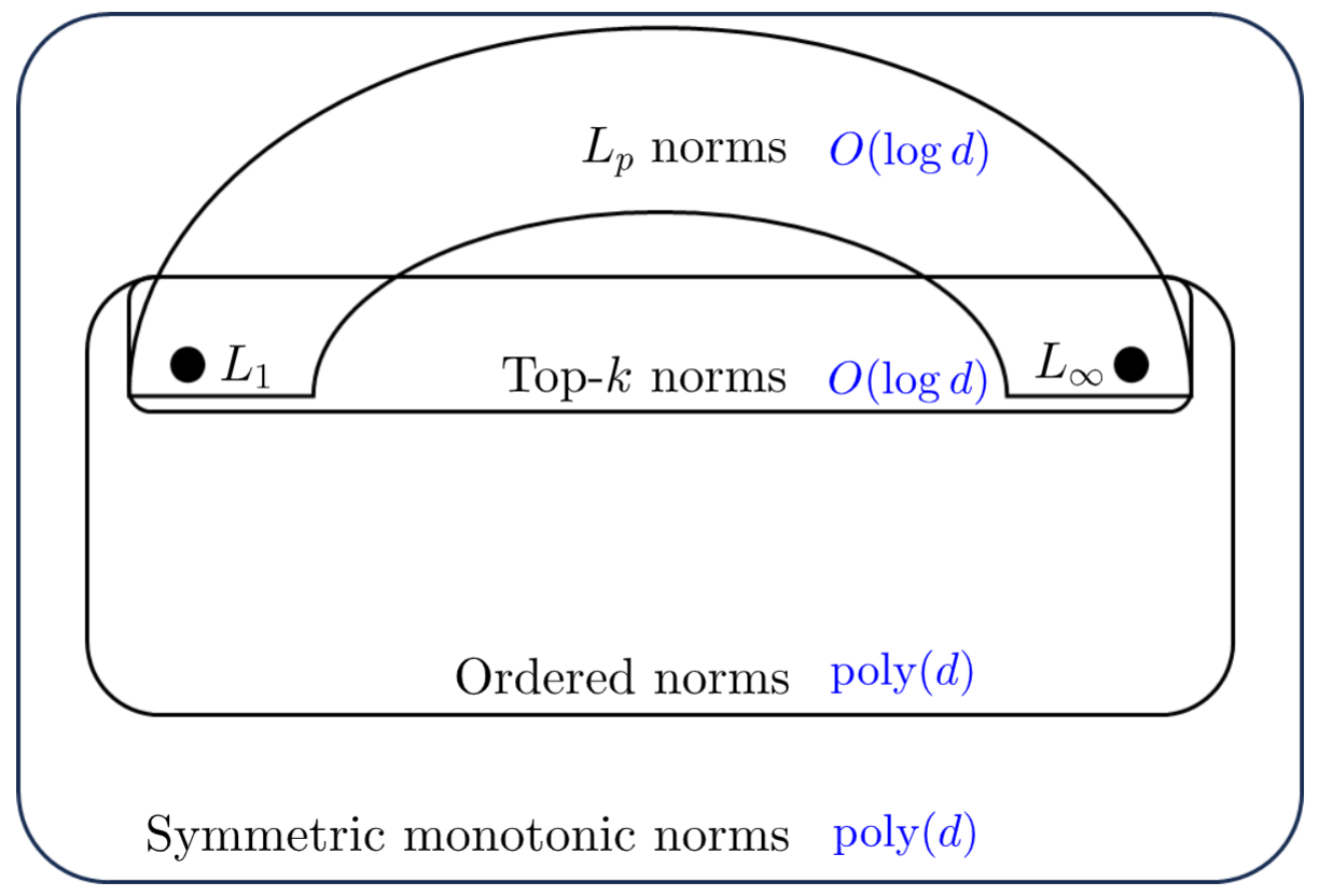
Figure 1: A Venn diagram for classes of norms discussed in this paper. (In blue) Upper bounds on sizes for any portfolios that are $O(1)$-approximations in dimension $d$ for arbitrary problems; note the gap between $L_{p}$ norms/top-$k$ norms, ordered norms, and all symmetric monotonic norms. The bound for $L_{p}$ norms is due to [23], the bound for top-$k$ norms is recorded in Observation 2, the bound for ordered norms is due to [12], and the bound for symmetric monotonic norms is recorded in Theorem 12.

• Existence of Size-1 Portfolios: Which combinatorial problems admit portfolios of size-$1$, i.e., a single solution that achieves a constant-factor approximation for all symmetric monotonic norms simultaneously?

• Portfolios of Size $>1$: If such a solution does not exist, what is the size of smallest portfolios for various combinatorial problems that achieve a constant-factor or logarithmic approximation for all symmetric monotonic norms?

• Computability: Finally, we study the computational question: can we find small portfolios efficiently?

These questions can also be considered from a polyhedral perspective. Many combinatorial problems are optimized at the vertices of certain combinatorial polyhedra (such as perfect matching polytope, path polyhedron etc). For example, in Section 3.1 on parallel scheduling with identical jobs, we seek a portfolio for the class $\mathcal{C}$ of all ordered norms over machine load vectors. We associate a polyhedron $\mathcal{P}$ with this problem, and show that it is sufficient to find a portfolio of vertices of $\mathcal{P}$ for the class $\mathcal{C}^{\prime}$ of linear functions. Indeed, a study of portfolios for combinatorial problems leads to new polyhedral questions as well.

1.1 Overview of results

We next give an overview of our results for a variety of settings. Based on portfolio size, our results and techniques fall into two categories: size-$1$ (Table 1) and size $>1$ (Table 2). Most of the portfolios we give are efficiently computable (i.e., all except the “ordered set cover” problem), but there can be a gap between the best-possible portfolio and what can be found in polynomial time.

Table 1: A summary of approximations for portfolios of size-$1$, i.e. simultaneous approximations.

Problem		Existence approximation	Polynomial-time obtainable approximation	Reference
$k$-clustering (bicriteria approximation) $n$ points	Previous work	$(3+\epsilon,O(\log n)+\frac{1}{\epsilon})$	$(9+\epsilon,O(\log n)+\frac{1}{\epsilon}$)	[33]
		$\left(1+\epsilon,O\left(\frac{\log n}{\epsilon}\right)\right)$	$\left(6+\epsilon,O\left(\frac{\log n}{\epsilon}\right)\right)$	[22]
	This work	$\left(1+\epsilon,O\left(\frac{\log n}{\epsilon}\right)\right)$	$\left(3+\epsilon,O\left(\frac{\log n}{\epsilon}\right)\right)$	Theorem 1
Parallel scheduling, job completion time minimization	This work	$4$	$8$	Theorem 4
Ordered set cover, $n$ ground set elements	Previous work	$O(\log n)$		[23]
	This work	$4$	-	Theorem 13

Table 2: A summary of approximations for portfolios of size $>1$. See also Figure 1. For each problem, the best possible simultaneous approximation using a single solution is square root in the problem dimension.

Problem	Best possible simultaneous approximation	Portfolio size	Approximation for ordered norms	Approximation for symmetric monotonic norms	Reference
Identical jobs scheduling, machine load minimization, $m$ machines	$\Omega(\sqrt{m})$	$O(\log m)$	$8$	$O(\log m)$	Theorems 5, 7
Minimum-norm point on hyperplane in dimension $d$	$\Omega(\sqrt{d})$	$O\left(\frac{\log d}{\epsilon}\right)$	$1+\epsilon$	$O(\log d)$	Theorem 10
Generalized facility location, $n$ points	$\Omega(\sqrt{n})$	$O\left(\log n\right)$	$O(\log n)$		Theorem 11

A simultaneous optimal solution for all norms (i.e. a size-$1$ optimal portfolio) is rare, as one might expect. It does exist for matroids: we observe in Appendix F that the greedy algorithm is optimal for all norms over the bases of the matroid. Additionally, we observe in Appendix G that this is also true when minimizing norms over submodular base polytope.

Result 1 (size-$1$ portfolios). An immediate next step is to relax the optimality criteria and allow for constant-factor approximation. Many of our new results here follow from an algorithmic framework called Iterative Covering inspired from ideas first used by [8]’s for the Minimum Latency Problem. It was shown to be $O(1)$-approximate for an all-norm Hamiltonian routing problem called ‘all-norm TSP’ [23, 18] and used for other problems in [23]. Our size-$1$ portfolio results include:

1. $k$-clustering (Section 2.1): Given a metric space, the problem here is to open $k$ centers to minimize the norm of the distances of points to their nearest open center. Using Iterative Covering, we give all-norm bicriteria approximation for $k$-clustering on $n$ points: $\left(1+\epsilon,O(\log n/\epsilon)\right)$ for existence and $\left(3+\epsilon,O(\log n/\epsilon)\right)$ for poly-time obtainable solutions (Theorem 2). The latter improves upon the previous results by [33] and [22] by constant factors.

2. Scheduling on parallel unidentical machines, job completion time minimization (Section 2.2): We consider the problem of minimizing the norm of the vector of job completion times on parallel machines. This generalizes the classical minimum total completion time (for $L_{1}$ norm) and minimum makespan (for $L_{\infty}$ norm) problems. Using Iterative Covering, we show the existence of a size-$1$ $4$-approximate portfolio and give a size-$1$ $8$-approximate portfolio in polynomial time (Theorem 4). This is the first such guarantee to the best of our knowledge. We also show that a better-than $1.13$-approximate portfolio of size-$1$ cannot exist (Appendix C, Theorem 15).

3. Scheduling on parallel identical machines, machine load minimization (Appendix D): In parallel scheduling, one can consider the analogous problem of minimizing the norm of machine loads instead. For identical machines, we show that the greedy algorithm gives a size-$1$ $3/2$-approximate portfolio for all symmetric monotonic norms (Theorem 16).

   This guarantee for the greedy algorithm was already known for $L_{p}$ norms as far back as 1975 ([14]); however, our analysis is significantly simpler and extends it to all norms. A PTAS for the best-possible approximation ratio [22] and a guarantee of $1.388$-approximation [3] for all norms exists; the greedy algorithm has a worse approximation but is simpler and faster; it runs in nearly linear time and has been the focus of previous works [24, 35, 14].

4. We consider the ordered set cover problem (Section B), where sets must be picked in an order and the cover time of an element is the first time a set covers it in this order. The problem is to minimize the norm of cover times. This generalizes both classic set cover and min-sum set cover (MSSC) ([4]). Using Iterative Covering, we show the existence of a size-$1$ $4$-approximate portfolio for this setting (Theorem 13); this stands in contrast to what can be obtained in polynomial-time: even classic set cover cannot be approximated to better than a logarithmic factor unless $P=NP$. [23] previously showed that the same framework also gives in polynomial-time a size-$1$ $O(\log n)$-approximation.

Result 2 (portfolios of size $>1$). In many cases, portfolios of size-$1$ with constant-factor or logarithmic approximations do not exist, and we seek ‘small’ portfolios instead. These results require new techniques, since many guarantees from size-1 portfolios break down in this setting. We first observe in Theorem 12 that an arbitrary set of vectors in dimension $d$ admits $O(1)$-approximate portfolio of size $\mathrm{poly}(d)$ for all symmetric monotonic norms; this is a simple extension of [12]’s technique for ordered norms. A next goal is to identify problems for which smaller portfolios exist; we give logarithmic portfolios of size $>1$ for the following problems (see Table 2 for a summary):

1. Scheduling on parallel unidentical machines with identical jobs, machine load minimization: we give $8$-approximate portfolio of size $1+\log_{2}m$ for all ordered norms (Section 3.1, Theorem 5). Using Corollary 1, these portfolios are also $O(\log m)$-approximate portfolios for all symmetric monotonic norms. We obtain this portfolio using convex relaxation and rounding. Moreover, we also give a lower bound showing instances where any portfolio that contains an $O(1)$-approximation for each ordered norm must have size at least $\widetilde{\Omega}(\log m)$ (Theorem 6).

2. Minimum-norm points on hyperplanes. Given a $d$-dimensional hyperplane, the problem is to find the minimum-norm point on this hyperplane, for various norms. Using a similar LP rounding technique, We show that there exist $O(1)$-approximate portfolios of size $O(\log d)$ for ordered norms (Section 3.2, Theorem 10). Using Corollary 1, these are also $O(\log d)$-approximate portfolios for all symmetric monotonic norms.

3. Uncapacitated facility location problem on $n$ points with uniform facility costs: given a metric space $(X,d)$ of demand points, the problem is to open some facilities in $X$ so as to minimize the sum of the number of open facilities and the norm of the distances of demand points to their nearest open facility. We give $O(\log n)$-approximate portfolio of size $O(\log n)$ for all symmetric monotonic norms (Section 2.1, Theorem 11). This follows from the guarantee for $k$-clustering described above.

1.2 Overview of techniques

Drawing from previous literature (e.g., [22]), we first note that for a combinatorial problem with the associated set of vectors $\mathcal{V}\subseteq\mathbb{R}^{d}_{\geq 0}$ and $\alpha\geq 1$, it is sufficient to give $x\in\mathcal{V}$ such that $x\preceq\alpha y$ for all $y\in\mathcal{V}$ to construct an $\alpha$-approximate portfolio. This is one of the key ideas that we use in our algorithms for size-$1$ portfolios.

Size-1 Portfolios: We propose Iterative Covering as a general algorithmic framework to find good size-1 portfolios. The high-level idea behind Iterative Covering that works for $k$-clustering, ordered set cover, and job completion time minimization is the following: we view the problem as a covering problem, and identify objects that cover items, with a cost associated with each object. The algorithm has multiple iterations, and each iteration intends to cover as many items as possible using objects with total cost bounded by a budget. These budgets increase exponentially with the iteration count. The problem-specific subroutine is then to combine the partial solutions obtained via different iterations to produce a single complete cover. The approximation guarantee depends on how well we can solve the subroutine in each iteration that covers items with objects within a given budget, and how we combine objects across iterations. The keys to the analysis are (1) to identify what notions of object, item, budget, and cost mean for each problem and (2) whether multiple objects can be combined together to get a single cover. While this framework has been used previously [23, 18], our main insights are that this approach is more widely applicable in non-trivial ways if we use the right building blocks, and that this algorithm gives existence results separate from polynomial time algorithmic results; a distinction missing from most previous work.

Size$>1$ Portfolios: If a portfolio of size-1 does not exist for a problem, then this presents interesting technical challenges. In particular, [22] show that an $\alpha$-approximate portfolio of size-$1$ for top-$k$ norms is also an $\alpha$-approximate portfolio for all symmetric monotonic norms. For size $1$-portfolios, this allows to restrict our attention to top-$k$-norms that are usually easier to handle. However, we show that this is not the case when the portfolio size is $>1$: we give instances for machine load minimization for parallel scheduling with $m$ machines that admit $O(1)$-approximate portfolios of size $2$ for top-$k$ norms but any $O(1)$-approximate portfolio for ordered norms must have size $\widetilde{\Omega}(\log m)$. Technically, the reduction fails since portfolio approximation for top-$k$ norms does not imply approximate majorization when portfolios of size $>1$ are allowed. Therefore, new techniques are needed when obtaining portfolios of larger size.

There is not much prior work in developing size $>1$ portfolios. For arbitrary sets of vectors, [23] essentially develop techniques that result in $O(1)$-approximate portfolios for $L_{p}$ norms; [28] make this explicit for facility location. [22]’s work implies $O(1)$-approximate logarithmic portfolios for top-$k$ norms. [12] essentially give $O(1)$-approximate portfolios of polynomial size for ordered norms.

First, we note that the problem of approximating over a given arbitrary set of vectors (Appendix A) follows from [12]’s technique for ordered norms and gives an $O(1)$-approximate portfolio of size $\mathrm{poly}(d)$ for all symmetric monotonic norms. The main question we ask is whether this polynomial dependence on $d$ can be improved. We answer this positively for few natural problems. We consider (i) identical job scheduling (Section 3.1) and (ii) finding a minimum norm portfolio of points over a d-dimensional hyperplane (section 3.2). For both these problems, we give $O(\log d)$-sized portfolios that achieve a good approximation. Minimizing an arbitrary norm can be formulated as a convex program and thus the optimal solution can be in the interior of the feasible region. To avoid approximating the possibly infinite, set of optimal solutions, one for each norm, we show that (approximately), this problem can be recast as a linear program. This allows us to focus on the vertices of the underlying polytope. While the number of vertices can be typically exponential in size, here the simple structure of the polytope allows us to bound it in a polynomial in $d$. To obtain the improved logarithmic bound, we use an additional doubling technique. For the identical jobs scheduling problem, we also need to round these vertices (that are fractional solutions) to integer solutions. However, the integrality gap is unbounded and not all vertices of this polytope can be rounded to a suitable integer point; we show using the underlying problem structure that these ‘bad’ vertices can be discarded. This technique shows the usefulness of the polyhedral view of portfolios.

Finally, we give (iii) $O(\log n)$-approximate portfolio of size $O(\log n)$ for the facility location problem (Section 3.3), using a simple extension of our result for $k$-clustering above.

1.3 Related work

Portfolios of size-$1$ (commonly known as simultaneous approximations) have been studied for various classes of objectives. [33] study simultaneous approximations for all norms for $k$-clustering, scheduling, and flow problems. In particular, for $k$-clustering, they show the existence of a bicriteria simultaneous $(3+\epsilon,O(\log n)+\epsilon^{-1})$-approximation and obtain a $(9+\epsilon,O(\log n)+\epsilon^{-1})$-approximation in polynomial time. [22] give a general framework for convex objectives and study $k$-clustering and scheduling in particular, giving a simultaneous bicriteria $(1+\epsilon,O((\log n)/\epsilon))$-approximation for $k$-clustering using a doubling technique and a polynomial-time simultaneous bicriteria $(6+\epsilon,O((\log n)/\epsilon)$-approximation using the rounding technique of [30]. They also give a PTAS for scheduling on identical machines. [3] prove that the this PTAS is in-fact a simultaneous $1.388$-approximation for all instances. [18] give a simultaneous approximation algorithm for a generalization of TSP. [23] study a large class of problems for simultaneous approximation for $L_{p}$ norms and all symmetric monotonic norms. [14] study scheduling with machine load minimization for $L_{p}$ norms.

Portfolios are not as well-studied as the above two problems; [23] and [28] study $L_{p}$ norm portfolios and [12] study portfolios for all ordered norms and give the $\mathrm{poly}(d)$ bound for $O(1)$-approximate portfolios in dimension $d$. The techniques for simultaneous approximation for $k$-clustering used in [22] essentially gives an $O(\log n)$ size $2$-approximate portfolio for top-$k$ norms for clustering.

Optimizing for a fixed non-standard objective has been widely considered in the literature. For example, [36, 21, 16] consider different $L_{p}$ norm objectives for $k$-clustering, [2, 34, 5, 13, 29] for scheduling problems, [18] for Hamiltonian routing and [23] for these and other problems. [11, 12] consider top-$k$ and ordered norms for $k$-clustering.

1.4 Preliminaries

In this section, we give various formal definitions and prove some useful lemmas. For vector $x\in\mathbb{R}_{\geq 0}^{d}$, $x^{\downarrow}$ is the vector with coordinates of $x$ sorted in decreasing order, i.e., $x^{\downarrow}_{1}\geq\ldots\geq x^{\downarrow}_{d}$. $x^{\uparrow}$ is similarly defined with the order reversed: $x^{\uparrow}_{1}\leq\ldots\leq x^{\uparrow}_{d}$. We define our norm classes and portfolios next:

Definition 1.

• Top-$k$ norm of $x$, denoted $\|x\|_{(\mathbf{1}_{k})}$, is the sum $x^{\downarrow}_{1}+\ldots+x^{\downarrow}_{k}$, i.e., the sum of $k$ highest coordinates of $x$. When $k=1$, it is the $L_{\infty}$ norm, and when $k=d$, it is the $L_{1}$ norm.

• An ordered norm on $\mathbb{R}^{d}$ is specified by a weight vector $w\in\mathbb{R}^{d}\setminus\{0\}$ satisfying $w_{1}\geq\ldots\geq w_{d}\geq 0$, and is defined as:

  $$\|x\|_{(w)}=w^{\top}x^{\downarrow}=\sum_{i\in[d]}w_{i}x^{\downarrow}_{i}.$$

  Notice that we recover the top-$k$ norm if we choose $w_{1}=\ldots=w_{k}=1$ and $w_{k+1}=\ldots=w_{d}=0$, so that top-$k$ norms are special cases of ordered norms. The set of all weight vectors in $d$ dimensions is denoted $\mathbf{W}_{d}=\{w\in\mathbb{R}_{\geq 0}^{d}:w_{1}\geq\ldots\geq w_{d}\geq 0,w\neq 0\}$.

• A symmetric monotonic norm $\|\cdot\|:\mathbb{R}_{\geq 0}^{d}\to\mathbb{R}_{\geq 0}$ is (a) a norm, (b) monotonic in each coordinate, and (c) symmetric, i.e., swapping any two coordinates of a vector does not change its norm value. Since this is the largest class of norms we consider, we will simply refer to these as all norms.

Definition 2 (Portfolios).

Given a set of vectors $\mathcal{V}\subseteq\mathbb{R}_{\geq 0}^{d}$ (e.g., vectors of machine loads in scheduling), a class of objectives $\mathcal{C}:\mathbb{R}_{\geq 0}^{d}\to\mathbb{R}_{\geq 0}$, and an approximation parameter $\alpha\geq 1$, a portfolio $X\subseteq\mathcal{V}$ is a set of vectors such that for all objectives $f\in\mathcal{C}$,

$$\min_{x\in X}f(x)\leq\alpha\min_{x\in\mathcal{V}}f(x),$$

that is, optimizing $f$ over $\mathcal{V}$ is the same as optimizing $f$ over $X$, up to a factor $\alpha$. When the portfolio has size-$1$, we call it a simultaneous approximation.

Informally, portfolios answer the following question: with respect to optimization for functions in $\mathcal{C}$, can we represent $\mathcal{V}$ by a smaller set $X$?

Usually, the set $\mathcal{V}$ is not specified explicitly, but is derived from an underlying combinatorial problem: it might represent the set of all distance vectors in $k$-clustering corresponding to different solutions. The size of $\mathcal{V}$ is usually exponential in the input size of the combinatorial problem, and therefore getting small portfolios is useful: it shows that a small set of solutions capture the essence of the combinatorial problem.

For $x,y\in\mathbb{R}_{\geq 0}^{d}$, we say that $y$ majorizes $x$ or $x\preceq y$ if $\sum_{i\leq[k]}x^{\downarrow}_{i}\leq\sum_{i\leq[k]}y^{\downarrow}_{i}$ for all $k\in[d]$. For a thorough treatment of majorization, see [7]. The first lemma connects symmetric norm values with majorization.

Lemma 1 ([22], Theorem 2.1).

If $x\preceq y$, then $\|x\|\leq\|y\|$ for any symmetric monotonic norm $\|\cdot\|$.

This helps us connect simultaneous approximation for top-$k$ to norms to simultaneous approximation for all norms: if $x^{*}$ is simultaneously $\alpha$-approximate for all top-$k$ norms over $\mathcal{V}$, then $\sum_{i\in[k]}x^{*}_{i}\leq\alpha\sum_{i\in[k]}y_{i}$ for all $k$ and $y\in\mathcal{V}$, or that $x\preceq\alpha y$ for all $y\in\mathcal{V}$. As an immediate consequence:

Observation 1 ([22], Theorem 2.3).

For any $\mathcal{V}\subseteq\mathbb{R}_{\geq 0}^{d}$, if $x^{*}$ is a simultaneous $\alpha$-approximation for all top-$k$ norms, then $x^{*}$ is a simultaneous $\alpha$-approximation for all norms.

For any $\mathcal{V}\subseteq\mathbb{R}_{\geq 0}^{d}$, a $(1+\epsilon)$-approximate portfolio for top-$k$ norms can be obtained by choosing optimal solutions corresponding to top-$k$ norms for $k=\lfloor 1+\epsilon\rfloor,\lfloor(1+\epsilon)^{2}\rfloor,\ldots$ . There are $\log_{1+\epsilon}(d)=O\left((\log d)/\epsilon\right)$ such values, and so:

Observation 2.

For any $\mathcal{V}\subseteq\mathbb{R}_{\geq 0}^{d}$ and $\epsilon\in(0,1]$, there exists a $(1+\epsilon)$-approximate portfolio of size $O\left(\frac{\log d}{\epsilon}\right)$ for all top-$k$ norms.

We remark that unlike Observation 1 for simultaneous optimization, portfolio guarantees do not carry over from top-$k$ norms to all norms. Indeed, despite the above observation for top-$k$ norms, the best-known upper bound for $O(1)$-approximate portfolio sizes for all symmetric monotonic norms is polynomial in $d$.

The next lemma allows symmetric monotonic norms to be $O(\log d)$-approximated by ordered norms; it will be useful to convert portfolios for ordered norms to portfolios for symmetric monotonic norms:

Lemma 2 ([37]).

Any symmetric monotonic norm $\|\cdot\|$ on $\mathbb{R}^{d}$ can be $O(\log d)$-approximated by an ordered norm on $\mathbb{R}^{d}$.

Corollary 1.

Given $\mathcal{V}\subseteq\mathbb{R}_{\geq 0}^{d}$, an $\alpha$-approximate portfolio $X$ for ordered norms over $\mathcal{V}$ is an $O(\alpha\log d)$-approximate portfolio for all symmetric monotonic norms over $\mathcal{V}$.

2 Size-1 Portfolios using Iterative Covering

We present simultaneous approximations for all norms for various problems using the Iterative Covering framework. Each of these problems can be informally seen as a covering problem where certain items need to be covered by some objects in some order, with possible constraints on the set of objects we can use. For example, consider job scheduling on parallel machines with several jobs to assign and machines to assign them on. Suppose we want to minimize some function of the job completion times. In this case, items are jobs, and objects are (job, machine) pairs indicating the machine a job will run on; each object covers a specific job. We need to cover all items (i.e. jobs) by selecting these objects. The order of selection of these objects indicates the order in which jobs will run on the machines.

Another example is $k$-clustering with the goal of minimizing some function of the distances of all points in the metric space. Items are the set of all points, and objects are sets of $k$ balls of a given radius. $k$ balls cover a point if it lies in their union. In the original application of this problem – Hamiltonian routings – the items are vertices, objects are edges, and the constraint on the edges is that they form a path. In set cover and related problems, the objects are naturally the sets themselves.

Our two insights are:

1. We show that the basic iterative structure of the algorithm works for a richer class of all-norm problems, and viewing the problem in the right way is often the key to modifying the algorithm suitably.

2. We also observe that the algorithm shows the existence of good solutions for all norms that may not be poly-time obtainable. For instance, in Appendix B, we give an algorithm with exponential runtime that shows the existence of simultaneous $4$-approximations for ordered set cover. This is surprising since such a solution can’t be found efficiently: even classic set cover cannot be approximated to within a factor $(1-o(1))\ln n$ unless $P=NP$. This further illuminates the gap between existence and algorithmic questions for all-norm problems. [23] observe that a simultaneous $O(\log n)$-approximation can be efficiently found with this framework.

We give simultaneous bicriteria approximation for $k$-clustering in the next subsection, improving upon the previous-best approximation for both existence and algorithmic problems. This also leads to a logarithmic-sized portfolio for uncapacitated facility location. We discuss scheduling for job completion time minimization in Section 2.2. We discuss ordered set cover and other applications in Appendix B.

2.1 Clustering

In this section, we consider generalized $k$-clustering. In this problem, we are given a metric space $(X,d)$ on $X=[n]$ points (also called clients) and are required to a subset $F\subseteq X$ of open facilities, and assign each client to its closest open facility. The induced distance vector $x=x(F)\in\mathbb{R}^{n}$ is defined as the vector of distances between point $j$ and its nearest open facility, i.e., $x_{j}=\min_{f\in F}d(j,f)$ for all $j\in X$.

Definition 3 (Generalized $k$-clustering).

Given integer $k$, we can open at most $k$ facilities, i.e., $|F|\leq k$. Given a norm $\|\cdot\|$, the corresponding objective is to find the set $F$ of open facilities that minimizes $\|x(F)\|$. For the top-$n$ norm, this is the $k$-median problem, and for the top-$1$ norm, this is the $k$-center problem.

A solution (similarly portfolio) is bicriteria $(\alpha,\beta)$-approximate with respect to an objective if it opens at most $\beta k$ facilities and its objective value is within factor $\alpha$ of the optimal solution with at most $k$ open facilities.

Given nonempty $F\subseteq X$ and some radius $R\geq 0$, we denote by $B(F;R)$ the set of all points within distance $R$ of $F$, i.e., $B(F;R)=\{x\in X:\exists\>y\in F\text{ with }d(x,y)\leq R\}$. We say that a set of facilities $F$ covers $p$ points within radius $R$ if $|B(F;R)|\geq p$.

The main results for this section is the following theorems which gives bicriteria simultaneous approximations for generalized $k$-clustering.

Theorem 2.

For the generalized $k$-clustering problem,

1. there exists a simultaneous bicriteria $\left(1+\epsilon,O\left(\frac{\log n}{\epsilon}\right)\right)$-approximation, and

2. a simultaneous bicriteria $\left(3+\epsilon,O\left(\frac{\log n}{\epsilon}\right)\right)$-approximation can be found in polynomial time.

We concretize Iterative Covering for generalized $k$-clustering as IterativeClustering (Algorithm 2).

We note that the part 1 of the theorem can also be obtained using Observation 2: take optimal $k$-clustering solutions corresponding to top-$l$ vectors for $l=\lfloor 1+\epsilon\rfloor,\lfloor(1+\epsilon)^{2}\rfloor,\ldots$ and combine these facilities to obtain a single solution with $O(k\log_{1+\epsilon}(n))$ facilities; this was noted for $\epsilon=1$ in [22]. For a polynomial-time bound, their technique of combining fractional solutions and rounding based on the techniques of [30] achieves a simultaneous $(6+\epsilon)$-approximation with $O(k\log_{1+\epsilon}n)$ facilities. For improved algorithmic approximation guarantee of $3+\epsilon$ (part 2 of the theorem), we need the idea of Iterative Covering, as we describe next:

At a high level, Algorithm IterativeClustering combines several solutions with $k$ facilities each. Each of these solutions corresponds to a radius $R$, and subroutine PartialClustering attempts to get the set of $k$ facilities that covers the largest number of points within radius $R$. Radius $R$ will increase exponentially across iterations.

For polynomial-time computations, PartialClustering cannot be solved exactly since it generalizes the $k$-center problem. To get efficient algorithms, we allow it to output $k$ facilities that cover as many points within radius $\alpha R$ as those covered by any $k$ facilities within radius $R$. [15] give an approximation algorithm for PartialClustering for $\alpha=3$, which we state in a modified form:

Theorem 3 (Theorem 3.1, [15]).

Given metric $(X,d)$, integer $k\geq 1$, and radius $R$, there exists a polynomial-time algorithm that outputs $k$ facilities that cover at least as many points within radius $3R$ as those covered by any set of $k$ facilities within radius $R$. That is, subroutine PartialClustering runs in polynomial-time for $\alpha=3$.

Let $D$ denote the $k$-center optimum for $(X,d)$. By definition, there are $k$ facilities that can cover all of $X$ within radius $D$. Therefore, the largest radius we need to consider is $D$. What is the smallest radius we need to consider? Since all of our objective norms are monotonic and symmetric, points covered within very small radii do not contribute a significant amount to the norm value. Therefore, we can start at a large enough radius, which has been set to $\frac{D\epsilon}{n}$ with some foresight.

Algorithm 1 PartialClustering($(X,d),k,R,\alpha$)

1:A metric space $(X,d)$, integer $k\geq 1$, radius $R\geq 0$, parameter $\alpha\geq 1$

2:A set of $k$ facilities $C\in\binom{X}{k}$ such that $B(C,\alpha R)$ contains at least as many points as contained by any $B(C^{\prime},R)$ with $|C^{\prime}|\leq k$, i.e.,

$$\left|B(C,\alpha R)\right|\geq\max_{C^{\prime}\in\binom{X}{k}}\left|B(C^{\prime},R)\right|.$$

Algorithm 2 IterativeClustering$((X,d),k,\epsilon,\alpha)$

1:A metric space $(X,d)$, integer $k\geq 1$, parameter $\epsilon>0$, parameter $\alpha\geq 1$

2:A set $C\subseteq X$ of $O\left(\frac{k\log n}{\epsilon}\right)$ facilities

3:$C\leftarrow\emptyset$

4:$R_{0}=\frac{D\epsilon}{n}$

5:for $l=0,1,\ldots,\log_{1+\epsilon}(n/\epsilon)$ do

6:     $R\leftarrow R_{0}(1+\epsilon)^{l}$

7:     $C_{l}\leftarrow\textsc{PartialClustering}((X,d),k,R,\alpha)$

8:     $C\leftarrow C\cup C_{l}$ return $C$

We will first prove the following claim:

Claim 1.

IterativeClustering gives a simultaneous bicriteria $\left(\alpha(1+2\epsilon),O\left(\frac{\log n}{\epsilon}\right)\right)$-approximation for generalized $k$-clustering.

Proof.

We first show that the number of facilities output by the algorithm is $O\left(\frac{k\log n}{\epsilon}\right)$. The number of iterations in the for loop is $\log_{(1+\epsilon)}\left(\frac{n}{\epsilon}\right)=O\left(\frac{\log n}{\epsilon}+\frac{\log(1/\epsilon)}{\epsilon}\right)$. When $\epsilon>\frac{1}{n}$, this expression is $O\left(\frac{\log n}{\epsilon}\right)$. Since each iteration adds at most $k$ facilities to $C$, we are done in this case. When $\epsilon\leq\frac{1}{n}$, then $\frac{k\log n}{\epsilon}\geq n$, that is, all facilities can be opened anyway.

Fix any symmetric monotonic norm $\|\cdot\|$ on $\mathbb{R}^{n}$, and let $\mathrm{OPT}$ denote the optimal solution for this norm and $x^{\mathrm{OPT}}\in\mathbb{R}^{n}$ denote the corresponding distance vector. Let the distance vector for facilities $C$ output by the algorithm be $x$. We need to show that $\|x\|\leq\alpha(1+2\epsilon)\|x^{\mathrm{OPT}}\|$.

By definition, $(x^{\mathrm{OPT}})^{\uparrow}_{1}\leq(x^{\mathrm{OPT}})^{\uparrow}_{2}\leq\ldots\leq(x^{\mathrm{OPT}})^{\uparrow}_{n}$. Let $j^{*}$ be the smallest index such that $(x^{\mathrm{OPT}})^{\uparrow}_{j^{*}}>R_{0}=\frac{D\epsilon}{n}$. Since $\|\cdot\|$ is symmetric, we have $\|x^{\uparrow}\|=\|x\|$ and $\|(x^{\mathrm{OPT}})^{\uparrow}\|=\|x^{\mathrm{OPT}}\|$. Our twofold strategy is to show that:

1. for all $j\geq j^{*}$,

   $$(x)^{\uparrow}_{j}\leq\alpha(1+\epsilon)(x^{\mathrm{OPT}})^{\uparrow}_{j},$$ (1)

2. the contribution of $x^{\uparrow}_{1},\ldots,x^{\uparrow}_{j^{*}-1}$ to $\|x\|$ is small; specifically,

   $$\left\|\left(x^{\uparrow}_{1},\ldots,x^{\uparrow}_{j^{*}-1},0,\ldots,0\right)\right\|\leq\alpha\epsilon\|x^{\mathrm{OPT}}\|.$$ (2)

Consider the first part. We have $R_{0}(1+\epsilon)^{\log_{1+\epsilon}(n/\epsilon)}=R_{0}\frac{n}{\epsilon}=D$. That is, in the final iteration of the for loop, $R=D$. Therefore, by definition of $D$ and PartialClustering, $C_{l}$ in this iteration covers all of $X$ within radius $\alpha D$. That is, $\|x\|_{\infty}\leq\alpha D$ since $C_{l}\subseteq C$.

fix some $j\geq j^{*}$, and let $l\geq 0$ be the smallest integer such that $(x^{\mathrm{OPT}})^{\uparrow}_{j}\leq R_{0}(1+\epsilon)^{l}$. If $l\geq 1+\log_{1+\epsilon}(n/\epsilon)$, then $(x^{\mathrm{OPT}})^{\uparrow}_{j}>R_{0}(1+\epsilon)^{l-1}=D$. Since $\|x\|_{\infty}\leq\alpha D$, inequality (1) holds in this case.

Otherwise, $l\leq\log_{1+\epsilon}(n/\epsilon)$. The $k$ facilities in $\mathrm{OPT}$ cover at least $j$ points within radius $R=R_{0}(1+\epsilon)^{l}$. By definition of PartialClustering, in iteration $l$ of the for loop, $C_{l}$ covers at least $j$ points within radius $\alpha R$. Since $C_{l}\subseteq C$, $C$ also covers at least $j$ points within radius $\alpha R$, so that $x^{\uparrow}_{j}\leq\alpha R=R_{0}(1+\epsilon)^{l}$. By definition of $l$, $(x^{\mathrm{OPT}})^{\uparrow}>R_{0}(1+\epsilon)^{l-1}$, and so

$$x^{\uparrow}_{j}\leq\alpha R_{0}(1+\epsilon)^{l}\leq\alpha(1+\epsilon)(x^{\mathrm{OPT}})^{\uparrow}_{j}.$$

We move to (2). By definition of $j^{*}$, $\mathrm{OPT}$ covers at least $j^{*}-1$ points within radius $R_{0}$. In iteration $0$, by definition of PartialClustering, $C_{0}$ (and therefore $C$) covers at least $(j^{*}-1)$ points within radius $\alpha R_{0}$. That is, $x^{\uparrow}_{j^{*}-1}\leq\alpha R_{0}$.

Denote $(1,0,\ldots,0)=\mathbf{e}$. Since $\|\cdot\|$ is monotonic and $D$ is the $k$ center optimum, $\|x^{\mathrm{OPT}}\|\geq\left(\|x^{\mathrm{OPT}}\|_{\infty},0,\ldots,0\right)\|\mathbf{e}\|\geq D\|\mathbf{e}\|$. Therefore,

$$\left\|\left(x^{\uparrow}_{1},\ldots,x^{\uparrow}_{j^{*}-1},0,\ldots,0\right)\right\| \leq\sum_{j\in[j^{*}-1]}x^{\uparrow}_{j}\|\mathbf{e}\| (\text{triangle inequality})$$

$$\leq\sum_{j\in[j^{*}-1]}\alpha R_{0}\|\mathbf{e}\| (x^{\uparrow}_{j^{*}-1}\leq\alpha R)$$

$$<n\alpha\frac{D\epsilon}{n}\|\mathbf{e}\| (j^{*}\leq n)$$

$$\leq\alpha\epsilon\|x^{\mathrm{OPT}}\|. (\|x^{\mathrm{OPT}}\|\geq D\|\mathbf{e}\|)$$

Together, inequalities (1), (2) imply that

$$\|x\| \leq\left\|\left(x_{1}^{\uparrow},\ldots,x^{\uparrow}_{j^{*}-1},0,\ldots,0\right)\right\|+\left\|\left(0,\ldots,0,x^{\uparrow}_{j^{*}},\ldots,x^{\uparrow}_{n}\right)\right\| (\text{triangle inequality})$$

$$\leq\alpha\epsilon\|x^{\mathrm{OPT}}\|+\alpha(1+\epsilon)\left\|\left(0,\ldots,0,(x^{\mathrm{OPT}})^{\uparrow}_{j^{*}},\ldots,(x^{\mathrm{OPT}})^{\uparrow}_{n}\right)\right\| (\text{inequalities }(\ref{eqn: clustering-pointwise-bound}),(\ref{eqn: clustering-bound-on-small-indices}))$$

$$\leq\alpha\epsilon\|x^{\mathrm{OPT}}\|+\alpha(1+\epsilon)\|x^{\mathrm{OPT}}\|=\alpha(1+2\epsilon)\|x^{\mathrm{OPT}}\|. (\|\cdot\|\text{ is symmetric monotonic})$$

∎

With this result in hand, we are ready to prove our main theorem:

Proof of Theorem 2.

1. Choose $\alpha=1$ in the claim with $\epsilon/2$ as the parameter.

2. Choose $\alpha=3$ in the claim with $\epsilon/6$ as the parameter. Theorem 3 guarantees that the algorithm is polynomial-time in the input size $n,\log\frac{1}{\epsilon}$.

∎

2.2 Parallel scheduling: job completion time minimization

In this section, we consider the job time minimization problem for parallel machines. We are given $n$ jobs and $m$ machines, with processing times $p_{i,j}$ for job $j\in[n]$ for machine $i\in[m]$. A feasible solution requires assigning each job to some machine (i.e., giving an assignment $\sigma:[n]\to[m]$) and then scheduling the jobs assigned to each machine in some order. Suppose jobs $j_{1},\ldots,j_{l}$ are assigned to some machine $i$ and scheduled in that order. Then the job completion time of job $j_{a}$ is $t_{j_{a}}:=\sum_{b\leq a}p_{i,j_{b}}$, i.e., the sum of processing times of jobs on $i$ scheduled before $j_{a}$ (including job $j_{a}$). The load $x_{i}$ for $i\in[m]$ is defined as the sum of processing times of jobs assigned to the machines, i.e.,

$$x_{i}=\sum_{j:\sigma(j)=i}p_{i,j}$$

The natural goal of minimizing the total (equivalently, average) job completion time $\sum_{j\in[n]}t_{j}$ has been extensively studied, and it can be solved in polynomial-time in our setting. Notice that this corresponds to the $L_{1}$ or top-$n$ norm of the job completion time vector $t\in\mathbb{R}^{n}$. Minimizing the $L_{\infty}$ norm of this vector is the same as minimizing the makespan or the maximum load on any machine. More generally, we can seek to minimize an arbitrary symmetric norm $\|t\|$; we call this the ordered parallel scheduling problem for job completion time minimization. We leave the other natural goal of minimizing norms of the machine load vector $x$ to Section 3.1, and focus on job completion times here.

We give another realization of Iterative Covering that shows the existence of a simultaneous $4$-approximation, and obtains in polynomial-time a simultaneous $8$-approximation for job completion times. We show in Appendix C that a simultaneous optimal solution cannot exist by giving a lower bound of $1.13$ on the best possible simultaneous approximation ratio (Theorem 15).

Theorem 4.

For the ordered scheduling problem for job completion time minimization,

1. there exists a simultaneous $4$-approximation, and

2. a simultaneous $8$-approximation can be found in polynomial-time.

First, we observe that any optimal solution for any norm schedules jobs on any given machine in increasing order of their processing times on that machine. This follows easily by an exchange argument; switching order of any two jobs that do not respect this ordering only improves the norm by a majorization argument (Lemma 1). Therefore, specifying just the assignment of jobs to machines is enough to specify a feasible schedule, with the scheduling order implied by the assignment.

A partial schedule is a feasible schedule for some subset of jobs $[n]$. A (partial) schedule with loads $L_{1},\ldots,L_{m}$ is said to take time $B$ if the makespan $\max_{i}L_{i}=B$. Makespan for partial schedules will be our notion of budget in the iterative algorithm. Two partial schedules can be combined in a natural way: for each machine, new jobs scheduled on the second partial schedule are appended to the jobs in the first partial schedule.

Algorithm IterativeScheduling keeps an exponentially increasing time budget $B$ in each iteration, with the aim of scheduling as many jobs as possible within this budget. This subroutine is called PartialScheduling; it has an additional parameter $\alpha$ that allows relaxing this budget to $\alpha B$. IterativeScheduling keeps iterating until budget $B$ is large enough that all jobs have been scheduled. The final schedule is obtained by appending the partial schedules from each iteration.

We will use the following result for PartialScheduling for the polynomial-time guarantee, proved in Appendix E:

Lemma 3.

There is a polynomial-time algorithm for PartialScheduling when $\alpha=2$.

Algorithm 3 PartialScheduling$(p,B,\alpha)$

1:Processing times $p_{i,j}$ for each job $j\in[n]$ and each machine $i\in[m]$, parameter $\alpha\geq 1$.

2:Partial job assignment $\sigma:[n]\to[m]$ with makespan $\leq\alpha B$ (i.e. $\sum_{j:\sigma(i)}p_{i,j}\leq\alpha B$ for all $i\in[m]$) and schedules at least as many jobs as any schedule with makespan $\leq B$.

Algorithm 4 IterativeScheduling($p$, $\alpha$)

1:Processing times $p_{i,j}$ for each job $j\in[n]$ and each machine $i\in[m]$, parameter $\alpha\geq 1$.

2:A job assignment to machines $\overline{\sigma}:[n]\to[m]$

3:Set ordering $C\leftarrow()$

4:Set partial assignment $\overline{\sigma}\leftarrow\emptyset$

5:for $l=0,1,\ldots$ do

6:     Set budget $B=2^{l}$

7:     $\sigma_{l}\leftarrow\textsc{PartialScheduling}(p,B,\alpha)$

8:     for each machine $i\in[m]$ do

9:         for each job $j\in[n]$ that is (1) unassigned under $\overline{\sigma}$ and (2) assigned to $i$ under $\sigma_{l}$, assign $\overline{\sigma}(j)=i$      

10:     exit loop if $\overline{\sigma}$ has scheduled all jobs, i.e., is a complete assignment return $\overline{\sigma}$

We proceed to prove the theorem. Fix a symmetric monotonic norm $\|\cdot\|$, and let $t^{\mathrm{OPT}}$ be the optimal completion time vector for this norm. We show that for the completion time vector $t$ for our algorithm, $t^{\uparrow}_{j}\leq 4\alpha\>(t^{\mathrm{OPT}})_{j}^{\uparrow}$ for all $j\in[n]$, implying that $\|t\|\leq 4\alpha\>\|t^{\mathrm{OPT}}\|$. Choosing $\alpha=1$ gives the existence result, and choosing $\alpha=2$ with Lemma 3 gives the poly-time result.

Fix $j\in[n]$, and let $l$ be the unique integer such that $2^{l-1}<(t^{\mathrm{OPT}})^{\uparrow}_{j}\leq 2^{l}$. Then, by definition of PartialScheduling, partial schedule $\sigma(l)$ in iteration $l$ of the loop assigns at least $j$ jobs. Since $\sigma$ iteratively assigns jobs from $\sigma(0),\sigma(1),\ldots$, the time $t^{\uparrow}_{j}$ is bounded above by the sum of makespans of $\sigma(0),\sigma(1),\ldots,\sigma(l)$:

$$t^{\uparrow}_{j}\leq\alpha 2^{0}+\ldots+\alpha 2^{l}<\alpha 2^{l+1}<4\alpha\>(t^{\mathrm{OPT}})^{\uparrow}_{j}.$$

3 Size $>1$ Portfolios

In this section, we give portfolios of size $>1$. We extend the enumeration technique of [12] to give $O(1)$-approximate portfolio of size $\mathrm{poly}(d)$ for arbitrary set of vectors in $d$ dimensions in Appendix A.

In Section 3.1, we consider machine load minimization in parallel scheduling with identical jobs, and give logarithmic sized portfolio. Using similar techniques, we deal with the case when the set of vectors $\mathcal{V}$ is a given hyperplane in Section 3.2: we give logarithmic sized portfolio of minimum-norm points on the hyperplane. In Section 3.3, we use our results on $k$-clustering to give logarithmic sized portfolio for uncapacitated facility location.

3.1 Parallel identical jobs scheduling: machine load minimization

Two problems deal with two fundamental aspects of parallel scheduling: whether we want to minimize some function of the machine loads (i.e., the total processing time of jobs assigned to each machine) or the job completion times. We can formulate the corresponding ordered norm and arbitrary norm problems for both these settings; we have already seen this for job completion time minimization in Section 2.2.

We now discuss the problem of minimizing norms of machine loads $x_{i},i\in[m]$. This generalizes classic makespan minimization for the $L_{\infty}$ norm. We handle the special case when all machines are identical in Appendix D, and show that [25]’s greedy algorithm gives simultaneous $3/2$-approximation (Theorem 16). For the rest of this section, we focus on the other special case when all jobs are identical, i.e., $p_{i,j}=p_{i}$ for all jobs $j\in[n]$ and machines $i\in[m]$.

Recall that job completion time minimization admits a single $4$-approximation for all symmetric monotonic norms. However, as we note later, when minimizing norms of machine loads, a single solution cannot be better-than simultaneous $O(\sqrt{m})$-approximation, even for the special case of identical jobs. In fact, we will show that in this case any constant-factor approximate portfolio must have size $\widetilde{\Omega}(\log m)$ (Theorem 6) even in this special case. Further, in this case, we can essentially match this bound: we give a size $1+\log_{2}m$ portfolio that is $8$-approximate for all ordered norms (Theorem 5) and $O(\log m)$-approximate for all symmetric monotonic norms (Theorem 7). See Tables 1, 2 for a summary of these results.

We can view the identical jobs scheduling problem alternately as follows: we need to schedule $n$ copies of a single job on unidentical machines. If $n_{i}\in\mathbb{Z}_{\geq 0}$ jobs are scheduled on machine $i$, then $\sum_{i}n_{i}=n$, and the load vector is $x=x(n)=(n_{1}p_{1},\ldots,n_{m}p_{m})$. The set of all possible load vectors is denoted $\cal{V}$. We prove the following results for this case:

Theorem 5.

There exists an $8$-approximate portfolio of size $1+\log_{2}m$ for all ordered norms for machine load minimization with identical jobs.

Theorem 6.

For all large enough $m$, there exists an instance of machine load minimization with identical jobs and $m$ machines where any constant-factor portfolio for all ordered norms has size $\widetilde{\Omega}(\log m)$.

The following immediately follows using Corollary 1:

Theorem 7.

There exists an $O(\log m)$-approximate portfolio of size $1+\log_{2}m$ for all symmetric monotonic norms for machine load minimization with identical jobs.

We can relabel the machine indices and assume that $p_{1}\leq\ldots\leq p_{m}$. Our first lemma shows that we can assume that each $p_{i}$ is a power of $2$, losing a factor $2$ in the approximation ratio. We call such instances doubling instances.

Lemma 4.

Given an instance of the identical jobs scheduling problem with $m$ machines and $n$ copies of a job, we can get a doubling instance of the problem with $m$ machines and $n$ jobs such that: for any load vector $x^{\prime}$ for this modified instance, the corresponding load vector $x$ for the original instance satisfies

$$\frac{1}{\sqrt{2}}x\leq x^{\prime}\leq\sqrt{2}x.$$

Proof.

To construct the new instance, round each $p_{i}$ to its closest power of $2$, say $p_{i}^{\prime}$. Then $\frac{1}{\sqrt{2}}p_{i}^{\prime}\leq p_{i}\leq\sqrt{2}p_{i}^{\prime}$. Consider load vectors $x^{\prime}=(n_{1}p_{1}^{\prime},\ldots,n_{m}p_{m}^{\prime})$ and $x=(n_{1}p_{1},\ldots,n_{m}p_{m})$; the lemma follows. ∎

We show that for doubling instances, optimal load vector $x^{\mathrm{OPT}}$ for any norm always satisfies the order $x^{\mathrm{OPT}}_{1}\geq\ldots\geq x^{\mathrm{OPT}}_{m}$; in particular, this implies that the ordered norm $\|x^{\mathrm{OPT}}\|_{(w)}$ is $\sum_{i}w_{i}x^{\mathrm{OPT}}_{i}$. This is not true if the instance is not doubling; see Figure 2. This is crucial since it will reduce a convex optimization problem to a linear one.

Lemma 5.

Suppose $x^{\mathrm{OPT}}$ is the optimal load vector for some symmetric monotonic norm $\|\cdot\|$ for a doubling instance. We can assume without loss of generality that $x^{\mathrm{OPT}}_{1}\geq x^{\mathrm{OPT}}_{2}\geq\ldots\geq x^{\mathrm{OPT}}_{m}$.

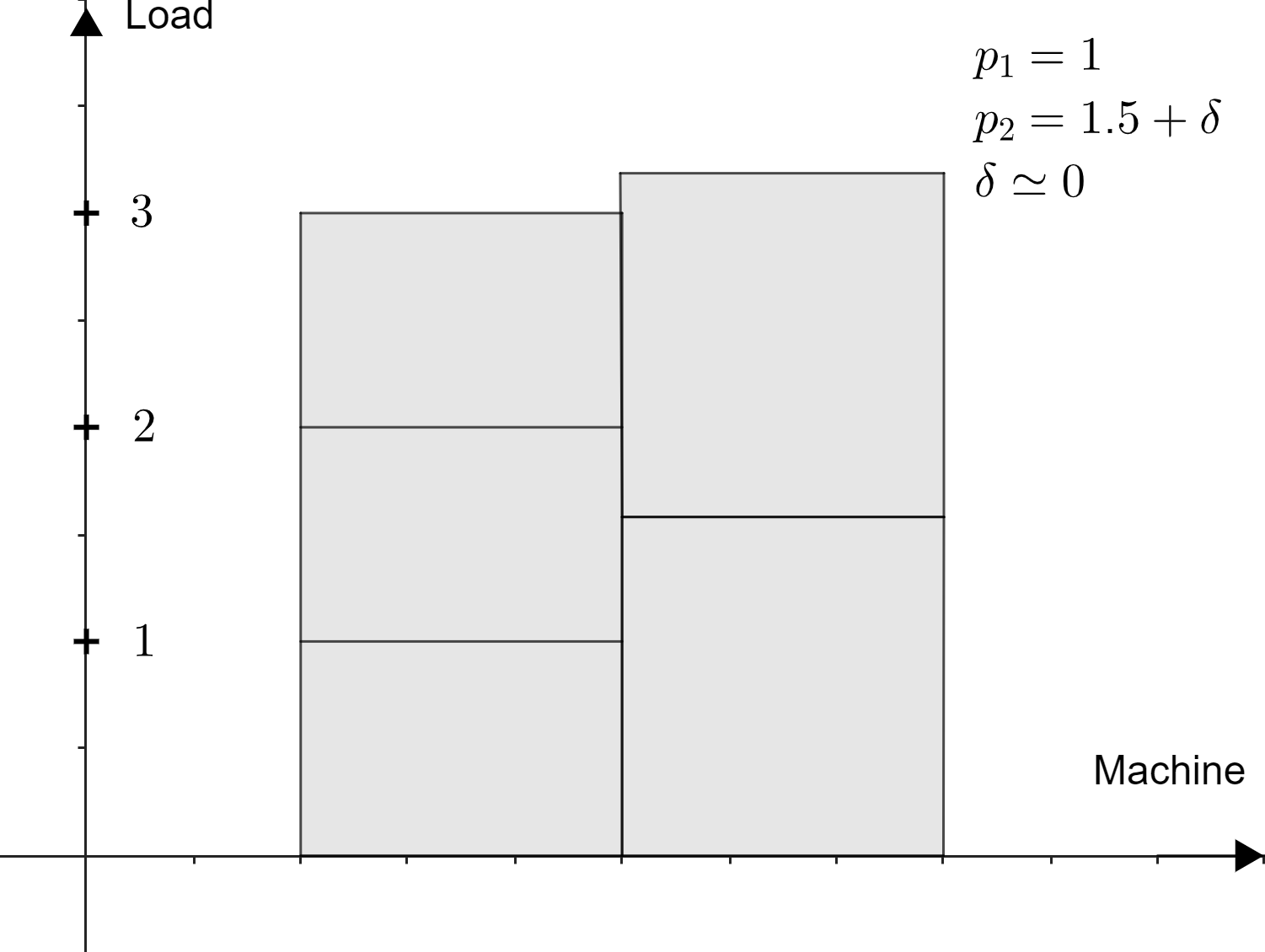
Figure 2: An example for makespan minimization with $2$ machines and $5$ jobs where $x^{\mathrm{OPT}}_{1}<x^{\mathrm{OPT}}_{2}$ for optimal $x^{\mathrm{OPT}}$.

Proof.

Suppose $x^{\mathrm{OPT}}_{i}<x^{\mathrm{OPT}}_{i+1}$ for some $i$. Transfer one job from machine $i+1$ to machine $i$, to get the new load vector $x$ defined as:

$$x_{l}=\begin{cases}x^{\mathrm{OPT}}_{l}&\text{if}\>l\neq i,i+1,\\ x^{\mathrm{OPT}}_{i}+p_{i}&\text{if}\>l=i,\\ x^{\mathrm{OPT}}_{i+1}-p_{i+1}&\text{if}\>l=i+1.\end{cases}$$

Since $p_{i}\mid p_{i+1}$, we get that $x^{\mathrm{OPT}}_{i+1}-x^{\mathrm{OPT}}_{i}\geq p_{i}$. Therefore,

$$\max(x_{i},x_{i+1})=\max\left(x^{\mathrm{OPT}}_{i}+p_{i},x^{\mathrm{OPT}}_{i+1}-p_{i+1}\right)\leq x^{\mathrm{OPT}}_{i+1}=\max\left(x^{\mathrm{OPT}}_{i},x^{\mathrm{OPT}}_{i+1}\right).$$

Further, $x_{i}+x_{i+1}<x^{\mathrm{OPT}}_{i}+x^{\mathrm{OPT}}_{i+1}$. That is, $(x_{i},x_{i+1})\prec(x^{\mathrm{OPT}}_{i},x^{\mathrm{OPT}}_{i+1})$. Since all other coordinates of $x$ and $x^{\mathrm{OPT}}$ are equal, a simple inductive argument shows that $x\prec x^{\mathrm{OPT}}$. Lemma 1 implies that $\|x\|\leq\|x^{\mathrm{OPT}}\|$, finishing the proof. ∎

Portfolio upper bound.

We focus on the upper bound (Theorem 5) first, giving an $8$-approximate portfolio of size at most $1+\log_{2}m$. Lemma 4 allows us to look only at doubling instances:

Corollary 8.

An $\alpha$-approximate portfolio for the identical jobs scheduling problem can be obtained from a $\frac{\alpha}{2}$-approximate portfolio for the corresponding doubling instance.

For the rest of this section, we restrict ourselves to doubling instances; we will give a $4$-approximate portfolio of size at most $1+\log_{2}m$ for all ordered norms for doubling instances.

For any weight vector $w\in\mathbf{W}_{m}$, the minimization problem for $\|\cdot\|_{(w)}$ can be formulated as the following integer program with a convex objective: $\min\|x\|_{(w)}$ under the constraints $\sum_{i}\frac{x_{i}}{p_{i}}=n$ and $\frac{x_{i}}{p_{i}}\in\mathbb{Z}_{\geq 0}$ for all $i$. The lemma above allows us to write an integer program (IP1) with a linear objective instead:

$$\min \>w^{\top}x$$ s.t. (IP1)

$$\sum_{i}\frac{x_{i}}{p_{i}} =n,$$ (3)

$$x_{i} \geq x_{i+1} \forall\>i\in[m-1].$$ (4)

$$\frac{x_{i}}{p_{i}} \in\mathbb{Z}_{\geq 0} \forall\>i\in[m].$$ (5)

$$\min \>w^{\top}x$$ s.t. (LP1)

$$\sum_{i}\frac{x_{i}}{p_{i}} =n,$$ (6)

$$x_{i} \geq x_{i+1} \forall\>i\in[m-1],$$ (7)

$$x \geq 0.$$ (8)

Each feasible solution to this integer program corresponds to a schedule/load vector, but not every load vector forms a feasible solution to it. However, Lemma 5 shows that there is an optimal solution that is feasible for this IP. Let us relax the integrality constraints in LP1.

Our strategy is as follows: the constraint polytope in LP1 has $m$ vertices, and we show that they can be approximated (in terms of majorization) by just $1+\log_{2}m$ of these vertices using sparsification. Some of these vertices can be rounded to integral schedules/load vectors (call these vertices good) losing a factor $2$, while other can’t. We will show that norm $\|\cdot\|_{(w)}$ of the optimal (integral) load vector can be improved by one of the good vertices. Since there are at most $1+\log_{2}m$ of them, we get a $1+\log_{2}m$ cardinality portfolio. The next lemma characterizes the optimal solutions to this LP, by characterizing the vertices of the constraint polytope:

Lemma 6.

For any weight vector $w$, the optimal solution $x^{*}$ to LP1 satisfies

$$x_{1}^{*} =\ldots=x_{l}^{*}=\frac{n}{\sum_{i\in[l]}\frac{1}{p_{i}}},$$

$$x^{*}_{l+1} =\ldots=x^{*}_{m}=0$$

for some index $l\in[m]$.

Proof.

$x^{*}$ corresponds to some vertex of the constraint polytope. Since there are $m+1$ constraints in total, there are (at most) $m+1$ vertices. It is easy to see that each vertex corresponds to an index $l$ such that $x^{*}_{1}=\ldots=x^{*}_{l}$, $x^{*}_{l+1}=\ldots=x_{m}^{*}=0$. Since $\sum_{i}\frac{x_{i}^{*}}{p_{i}}=n$, we get $x^{*}_{1}=\ldots=x^{*}_{l}=\frac{n}{\sum_{i\in[l]}\frac{1}{p_{i}}}$. ∎

Denote the vertex corresponding to the $l$th index as $x(l)$:

$$x(l)=\bigg{(}\underbrace{\frac{n}{\sum_{i\in[l]}\frac{1}{p_{i}}},\ldots,\frac{n}{\sum_{i\in[l]}\frac{1}{p_{i}}}}_{l},0,\ldots,0\bigg{)}.$$

Call $x(l)$ good if

$$\frac{n}{\sum_{i\in[l]}\frac{1}{p_{i}}}\geq p_{l},$$ (9)

i.e., the value of each non-zero coordinate is at least the processing time corresponding to the last non-zero coordinate. Clearly, $x(1)$ is good since $n\geq 1$, and if $x(l)$ is good then $x(l-1)$ is also good. Let $L$ be the largest index such that $x(L)$ is good. The next lemma says that if $x(l)$ is good, then it can be rounded to an integral load vector:

Lemma 7.

If $x(l)$ is good, then it can be rounded to $\hat{x}(l)$ that is feasible for IP1 and $\frac{1}{2}x(l)\leq\hat{x}(l)\leq 2x(l)$.

Proof.

Denote $n_{i}=\frac{x(l)_{i}}{p_{i}}$ for all $i\in[m]$, then $n_{l+1}=\ldots=n_{m}=0$ and $\sum_{i\in[m]}n_{i}=n$. Then one can assign either $\hat{n}_{i}=\lfloor n_{i}\rfloor$ or $\hat{n}_{i}=\lceil n_{i}\rceil$ jobs to machine $i\in[m]$, while ensuring that $\sum_{i\in[m]}\hat{n}_{i}=n$. The load on machine $i\in[m]$ in this new schedule is $\hat{x}(l)$, with $\hat{x}(l)_{i}=p_{i}\hat{n}_{i}$.

By definition of good vertices, $x(l)_{i}\geq p_{l}\geq p_{i}$ for each $i\in[l]$. Therefore, we get $n_{i}\geq 1$, thus implying $\frac{1}{2}n_{i}\leq\lfloor n_{i}\rfloor\leq n_{i}$ and $n_{i}\leq\lceil n_{i}\rceil\leq 2n_{i}$ for all $i\in[l]$. This implies $\frac{1}{2}n_{i}\leq\hat{n}_{i}\leq 2n_{i}$ for all $i\in[m]$. Since $n_{i}=\frac{x(l)_{i}}{p_{i}}$ and $\hat{n}_{i}=\frac{\hat{x}(l)_{i}}{p_{i}}$, we get the result. ∎

Lemma 8.

$\{\hat{x}(1),\ldots,\hat{x}(L)\}$ is a $4$-approximate portfolio for all ordered norms for the doubling instance.

Proof.

Fix a weight vector $w\in\mathbf{W}_{m}$. Let $x^{\mathrm{OPT}}$ be the optimal load vector for $\|\cdot\|_{(w)}$, and let $l$ be the largest index such that $x^{\mathrm{OPT}}_{l}>0$. We will show that there exists an index $l^{\prime}\leq l$ such that (1) $x(l^{\prime})$ is good, and (2) $\|x(l^{\prime})\|_{(w)}\leq\|x^{\mathrm{OPT}}\|_{(w)}$. Together with Lemma 7, this implies that $\|\hat{x}(l^{\prime})\|_{(w)}\leq 2\|x^{\mathrm{OPT}}\|_{(w)}$, implying the lemma.

We first show that $x(l)$ is good, which implies that $x(l^{\prime})$ is good for all $l^{\prime}\leq l$. Since $x^{\mathrm{OPT}}$ is integral and $x^{\mathrm{OPT}}_{l}\neq 0$, $x^{\mathrm{OPT}}_{l}\geq p_{l}$. From Lemma 5, $x^{\mathrm{OPT}}_{1}\geq\ldots\geq x^{\mathrm{OPT}}_{l}\geq p_{l}$. Since $\sum_{i\in[l]}\frac{x^{\mathrm{OPT}}_{i}}{p_{i}}=n$, we get $n\geq\sum_{i\in[l]}\frac{p_{l}}{p_{i}}=p_{l}\sum_{i\in[l]}\frac{1}{p_{i}}$. That is, $x(l)$ is good.

In particular, this implies that $x(l^{\prime})$ is good for each $l^{\prime}\leq l$, so it is now sufficient to show that there is some $l^{\prime}\leq l$ such that $\|x(l^{\prime})\|_{(w)}\leq\|x^{\mathrm{OPT}}\|_{(w)}$. To show this, consider the following linear program:

$$\min \>w^{\top}x$$ s.t. (LP2)

$$\sum_{i}\frac{x_{i}}{p_{i}} =n,$$ (10)

$$x_{i} \geq x_{i+1} \forall\>i\in[m-1],$$ (11)

$$x_{l+1} =\ldots=x_{m}=0.$$ (12)

$x^{\mathrm{OPT}}$ is feasible for this LP by assumption. Further, by an argument similar to Lemma 6, we get that the vertices of the constraint polytope for this LP are $x(1),\ldots,x(l)$. Therefore, there is some $l^{\prime}\leq l$ such that $\|x(l^{\prime})\|_{(w)}=w^{\top}x(l^{\prime})\leq w^{\top}x^{\mathrm{OPT}}=\|x^{\mathrm{OPT}}\|_{(w)}$, finishing the proof. ∎

We are now ready to prove Theorem 5.

Proof of Theorem 5.

For any doubling instance, we have $2$-approximate portfolios of size $m$. We will convert this to $4$-approximate portfolios of size $\sim\log_{2}m$ for doubling instances, which implies $8$-approximate portfolios of size $\sim\log m$ for identical jobs scheduling by Corollary 8.

We show that for all $l\in[m/2]$ and $i\leq 2l$, $x(l)\preceq x(i)$. Therefore, $\|x(l)\|_{(w)}\leq 2\|x(i)\|_{(w)}$ for all $w\in\mathbf{W}_{m}$ from Lemma 1, implying that $\left\{x(2^{0}),x(2^{1}),x(2^{2}),\ldots,x(2^{\lfloor\log L\rfloor})\right\}$ is a $4$-approximate portfolio. $L\leq m$ gives $1+\lfloor\log_{2}L\rfloor\leq 1+\log_{2}m$.

Since $p_{1}\leq\ldots\leq p_{n}$ and $i\leq 2l$, we have $\sum_{j\in[l]}\frac{1}{p_{j}}\geq\frac{1}{2}\sum_{j\in[i]}\frac{1}{p_{j}}$. Therefore, for all $k\leq l$, we have

$$\sum_{j\in[k]}x(l)_{j}=\frac{kn}{\sum_{i\in[l]}\frac{1}{p_{j}}}\leq\frac{2kn}{\sum_{j\in[i]}\frac{1}{p_{j}}}=2\sum_{j\in[k]}x(i)_{k}.$$

Further, for $k>l$,

$$\sum_{j\in[k]}x(l)_{j}=\sum_{j\in[l]}x(l)_{j}\leq 2\sum_{j\in[l]}x(i)_{j}\leq\sum_{j\in[k]}x(l)_{j}=2\sum_{j\in[l]}x(l)_{j}\leq 2\sum_{j\in[k]}x(i)_{j}.$$

Therefore, $x(l)\preceq 2x(i)$. This completes the proof. ∎

Portfolio lower bound.

We prove Theorem 6 by giving a doubling instance such that every $O(1)$-approximate portfolio for all ordered norms for this instance must have size $\widetilde{\Omega}(\log m)$.

As warm-up, we first give instances where a single solution can be an $\Omega(\sqrt{m})$-approximation at best. Suppose there are $m$ machines and $m$ jobs, and $p_{1}=1$ while $p_{i}=\sqrt{m}$ for all $i\geq m$. Then the optimal schedule for $L_{1}$ norm schedules all jobs on machine $1$, with $L_{1}$ norm $m$. The optimal $L_{\infty}$ norm is $\sqrt{m}$, obtained for example by scheduling one job on each machine. However, any schedule that schedules $\leq m/2$ jobs on machine 1 has $L_{1}$ norm $\Omega(m\sqrt{m})$. But any schedule that schedules more than $m/2$ jobs on machine $1$ has $L_{\infty}$ norm $\Omega(m)$.

Since two weight vectors that are scalar multiples of each other correspond to the same norm, we use a convenient normalization for weight vector for this proof: we assume $w_{1}=1$ for $w\in\mathbf{W}_{m}$.

We describe the instance on $m$ machines. Given $m$, let $S=S(m)$ be a superconstant that we specify later; assume that $S$ is an integer that is a power of $2$. Let $L$ be the largest integer such that $1+S^{2}+\ldots+S^{2L}\leq m$, then $L=\Theta(\log_{S}m)$. The $m$ machines are are divided into $L+1$ classes from $0$ to $L$: there are $S^{2l}$ machines in the $l$th class and the processing time on these machines is $p_{l}=S^{l}$.

The number of jobs $n$ is $S^{3L}$; it is chosen so as to ensure that all vertices in the constraint polytope for LP1 are good, and can be rounded to an integral solution that is only worse by a factor at most $2$ (Lemma 7).

There are $L+1$ weight vectors for our instance. The first weight vector is $w(0)=(1,1,\ldots,1)$. The second weight vector is $w(1)=\left(1,\frac{1}{S^{2}},\frac{1}{S^{2}},\ldots,\frac{1}{S^{2}}\right)$. More generally, for $l\in[0,L]$,

$$w(l)=\bigg{(}1,\underbrace{\frac{1}{S^{2}},\ldots,\frac{1}{S^{2}}}_{S^{2}},\underbrace{\frac{1}{S^{4}},\ldots,\frac{1}{S^{4}}}_{S^{4}},\ldots,\underbrace{\frac{1}{S^{2l-2}},\ldots,\frac{1}{S^{2l-2}}}_{S^{2l-2}},\underbrace{\frac{1}{S^{2l}},\ldots,\frac{1}{S^{2l}}}_{\text{remaining}}\bigg{)}.$$

Choose $S$ so that asymptotically $S=L\log L$, this implies $L=o(S)$. We will show the following claims: for each $l\in[0,L]$,

1. There is a schedule $\hat{x}(l)$ for this instance with $\|\hat{x}(l)\|_{(w(l))}=\Theta(nlS^{-l})$.

2. Any schedule $y$ that schedules more than $n/4$ jobs on machines in classes $l+1$ to $L$ has $\|y\|_{(w(l))}=\omega(nlS^{-l})$. Combined with the above, it cannot be a constant-factor approximation for the $w(l)$-norm problem.

3. Any schedule $y$ that schedules more than $n/4$ jobs on machines in classes $0$ to $l-1$ has $\|y\|_{(w(l))}=\omega(nlS^{-l})$. Therefore, it cannot be a constant-factor approximation for the $w(l)$-norm problem either.

4. $L=\Theta(\log_{S}m)=\widetilde{\Omega}(\log m)$.

Claims 1, 2, and 3 imply that any $O(1)$-approximate solution for norm $w(l)$ must schedule at least $n/2$ jobs on machines in class $l$. Another application of claims 2 and 3 then implies that a portfolio that is $O(1)$-approximate for weight vectors $\{w(0),\ldots,w(L)\}$ must have distinct solutions for each weight vector, and therefore has size at least $L+1$. Claim 4 then implies our theorem.

Claim 4 is simple computation: $L=\Theta(\log_{S}m)$, and since $S=L\log L$, we get $\Theta(\log m)=L\log L\log\log L$, and so $L=\widetilde{\Omega}(\log m)$ (since $\log L$ and smaller terms can be ignored under $\widetilde{\Omega}$).

We move to claim 1. As alluded to before, $n=S^{3L}$ has been chosen so that each vertex $x(l)$ of the constraint polytope is good (see inequality (9)):

$$\frac{n}{1\cdot\frac{1}{1}+S^{2}\cdot\frac{1}{S}+\ldots+S^{2L}\cdot\frac{1}{S^{L}}}\geq\frac{n}{2S^{L}}\geq S^{L}=p_{L}.$$

With this in hand, it is sufficient to give a fractional solution $x(l)$ with $\|x(l)\|_{(w(l))}=\Theta(nlS^{-l})$, since Lemma 7 then implies the existence of an integral solution $\hat{x}(l)$ with norm at most twice.

Consider $x(l)=\left(a,\ldots,a,0,\ldots,0\right)$ where the first $1+S^{2}+\ldots+S^{2l}$ coordinates are non-zero and equal to $a$; all other coordinates are $0$. Since a total of $n$ jobs must be scheduled (constraint (10)),

$$n=a\left(1\cdot\frac{1}{1}+S^{2}\cdot\frac{1}{S}+\ldots+S^{2l}\cdot\frac{1}{S^{l}}\right)\geq aS^{l},$$

so that $a\leq\frac{n}{S^{l}}$. Therefore,

$$\|x(l)\|_{(w(l))}=a\times\text{ sum of first }(1+S^{2}+\ldots+S^{2l})\text{ coordinates of }w(l)=a\cdot l\leq nlS^{-l}.$$

We move to claim 2. Let $y$ schedule more than $n/4$ jobs on machines in classes $l+1$ to $L$. Irrespective of how these $n/4$ jobs are distributed, they contribute a total load of at least $(n/4)\times S^{l+1}=\Theta(nS^{l+1})$. Since all coordinates of $w(l)$ are at least $\frac{1}{S^{2l}}$, the contribution of these jobs to $\|y\|_{(w(l))}$ is at least

$$\frac{1}{S^{2l}}\Theta(nS^{l+1})=\Theta(nS\cdot S^{-l}).$$

Since $l\leq L=o(S)$, we get $\|y\|_{(w(l))}=\omega(nlS^{-l})$.

Finally, we prove claim 3. Consider the restricted instance with only machines from classes $0,\ldots,l-1$ and $n/4$ jobs. Let $x$ be the optimal fractional solution for this instance for top-$1$ norm $\|\cdot\|_{(\mathbf{1}_{1})}$; it is easy to see that $x$ must have equal loads on machines, so that from constraint (10):

$$n=\|x\|_{(\mathbf{1}_{1})}\left(1\cdot\frac{1}{1}+S^{2}\cdot\frac{1}{S}+\ldots+S^{2l-2}\cdot\frac{1}{S^{l-1}}\right)\leq 2\|x\|_{(\mathbf{1}_{1})}S^{l-1},$$

implying $\|x\|_{(\mathbf{1}_{1})}\geq\frac{nS^{-l+1}}{2}$. Therefore, any integral optimal solution $\hat{x}$ to this restricted instance must also satisfy

$$\|\hat{x}\|_{(\mathbf{1}_{1})}\geq\|x\|_{(\mathbf{1}_{1})}\geq\frac{nS^{-l+1}}{2}.$$

Since $y$ is a solution to the larger original instance, we have $\|y\|_{(\mathbf{1}_{1})}\geq\|\hat{x}\|_{(\mathbf{1}_{1})}$. Finally, since $w(l)=1$ by assumption, we get $\mathbf{1}_{1}\preceq w(l)$, and so $\|y\|_{(w(l))}\geq\|y\|_{(\mathbf{1}_{1})}$. Together, we get $\|y\|_{(w(l))}=\Omega(nS\cdot S^{-l})=\omega(nlS^{-l})$. This completes the proof of the claim, and of Theorem 6.

Portfolios for different classes of norms.

Recall Observation 1: if $x^{*}$ is a simultaneous $\alpha$-approximation for each top-$k$ norm, then it is a simultaneous $\alpha$-approximation for all symmetric monotonic norms. One might naturally wonder if this is true for portfolio: is an $\alpha$-approximate portfolio for top-$k$ norms also an $\alpha$-approximate portfolio for all symmetric monotonic norms? We show that this is false, and that in fact portfolios for even ordered norms can be much larger than portfolios for top-$k$ norms:

Theorem 9.

For all large enough $d$, there exists a set of vectors $\mathcal{V}\subseteq\mathbb{R}_{\geq 0}^{d}$ such that:

1. there is an $O(1)$-approximate portfolio $X$ of size $2$ for all top-$k$ norms, and

2. any $O(1)$-approximate portfolio $X^{\prime}$ for all ordered norms has size $\widetilde{\Omega}\left(\log d\right)$.

Proof of Theorem 9.

We show that all instances of identical jobs scheduling problem with $m$ machines admit $O(1)$-approximate portfolio of size $2$ for all top-$k$ norms. Recall that theorem 6 gives instances where any $O(1)$-approximate portfolio for ordered norms must have size $\widetilde{\Omega}(\log m)$. Combined, this implies the result with $m=d$.

Recall Lemmas 8, 7: $X^{\prime}=\{\hat{x}(1),\ldots,\hat{x}(L)\}$ is an $O(1)$-approximate portfolio for all ordered norms where $\frac{1}{2}x(l)\leq\hat{x}(l)\leq 2x(l)$ for all $l\in[L]$. Therefore, $\|\hat{x}(l)\|_{\mathbf{1}_{k}}$ is within factor $2$ of $\|x(l)\|_{\mathbf{1}_{k}}$ for all $k\in[m]$. Further for all $k\in[m]$,

$$\|x(l)\|_{\mathbf{1}_{k}}=\begin{cases}\frac{ln}{\sum_{i\in[l]}\frac{1}{p_{i}}}&\text{if}\>l\leq k,\\ \frac{kn}{\sum_{i\in[l]}\frac{1}{p_{i}}}&\text{if}\>l>k.\end{cases}$$

Fix $k$. Since $p_{i}\leq p_{i+1}$ for all $i$, $\frac{ln}{\sum_{i\in[l]}\frac{1}{p_{i}}}$ is non-increasing in $l$. Further, $\frac{kn}{\sum_{i\in[l]}\frac{1}{p_{i}}}$ is decreasing in $l$. Therefore, the smallest among $\|x(l)\|_{\mathbf{1}_{k}},l\in[L]$ is either $\|x(1)\|_{\mathbf{1}_{k}}$ or $\|x(L)\|_{\mathbf{1}_{k}}$. Therefore,

$$\min\{\|\hat{x}(1)\|_{\mathbf{1}_{k}},\|\hat{x}(l)\|_{\mathbf{1}_{k}}\} \leq 2\min\{\|{x}(1)\|_{\mathbf{1}_{k}},\|{x}(l)\|_{\mathbf{1}_{k}}\}$$

$$\leq 2\min\{\|{x}(1)\|_{\mathbf{1}_{k}},\|{x}(2)\|_{\mathbf{1}_{k}},\ldots,\|{x}(L)\|_{\mathbf{1}_{k}}\}$$

$$\leq 4\min\{\|\hat{x}(1)\|_{\mathbf{1}_{k}},\|\hat{x}(2)\|_{\mathbf{1}_{k}},\ldots,\|\hat{x}(L)\|_{\mathbf{1}_{k}}\}.$$

Since $\{\hat{x}(1),\ldots,\hat{x}(L)\}$ is an $O(1)$-approximate portfolio for all ordered norms, this implies that $\{\hat{x}(1),\hat{x}(L)\}$ is an $O(1)$-approximate portfolio for all top-$k$ norms. ∎

We can also show that portfolios for ordered norms are not portfolios for $L_{p}$ norms: consider an instance of identical jobs scheduling with $p_{i}=\sqrt{i}$ for each $i\in[m]$. Denote $\rho(l)=\sum_{i\in[l]}\frac{1}{p_{i}}=\sum_{i\in[l]}\frac{1}{\sqrt{i}}$; also denote the $m$th Harmonic number $H_{m}=\sum_{i\in[m]}\frac{1}{i}=\Theta(\log m)$. Then for each $l\in[m]$, $x(l)=\Big{(}\underbrace{\frac{n}{\rho(l)},\ldots,\frac{n}{\rho(l)}}_{l},0,\ldots,0\Big{)}$. Recall (Lemmas 7, 8) that there exists an $L\in[m]$ such that (1) $\frac{1}{2}x(l)\leq\hat{x}(l)\leq 2x(l)$ for all $l\in[L]$ and (2) $X^{\prime}=\{\hat{x}(1),\ldots,\hat{x}(L)\}$ is an $O(1)$-approximate portfolio for ordered norms for some $L\in[m]$. We claim that each $x\in Xl$ is an $\Omega(\sqrt{H_{m}})$-approximation for the $L_{2}$ norm.

For each $l\in[L]$, $\rho(l)\leq 1+2\int_{1}^{l}\frac{2}{\sqrt{x}}\leq 4\sqrt{l}$, so that

$$2\|\hat{x}(l)\|_{2}\geq\|x(l)\|_{2}=\frac{n}{\rho(l)}\cdot\sqrt{l}\geq\frac{n}{4}.$$

Consider the following assignment: assign $n_{i}=\frac{n}{iH_{m}}$ jobs to machine $i\in[m]$, and choose $n$ large enough so that each $n_{i}$ is integral. Then this is a valid assignment since $\sum_{i\in[m]}n_{i}=n$ by definition of $H_{m}$. The machine loads for this assignment are $x_{i}=n_{i}p_{i}=\frac{n}{H_{m}\sqrt{i}}$. The $L_{2}$ norm of $x$ is

$$\|x\|_{2}=\frac{n}{H_{m}}\sqrt{\sum_{i\in[m]}\frac{1}{i}}=\frac{n}{\sqrt{H_{m}}}.$$

Therefore, each $\hat{x}(l)$ is an $\Omega(\sqrt{H_{m}})$-approximation for the $L_{2}$ norm.

3.2 Logarithmic portfolio for hyperplanes

The identical jobs problem imposes two constraints on loads $x_{i}$: that $\frac{x_{i}}{p_{i}}$ should be integral and $\sum_{i}\frac{x_{i}}{p_{i}}=n$. We dealt with the first constraint using a convex relaxation and then rounding fractional solutions. However, the techniques used give a recipe to get portfolios for a hyperplane $H=\{x\in\mathbb{R}^{d}:\sum_{i\in[d]}a_{i}x_{i}=1\}$ for a non-zero given vector $a\in\mathbb{R}^{d}$. Formally, we prove the following theorem:

Theorem 10.

Given a hyperplane $H=\{x\in\mathbb{R}^{d}:a^{\top}x=1\}$ in $\mathbb{R}^{d}$ and $\epsilon>0$, there exists a $(1+\epsilon)$-approximate portfolio $X\subseteq H$ with $|X|=O\left(\frac{\log d}{\epsilon}\right)$ for all ordered norms. Further, this portfolio is $O\left(\log d\right)$-approximate for all symmetric monotonic norms.

The statement for symmetric monotonic norms follows from the statement for ordered norms using Corollary 1; we focus on ordered norms hereafter.

Since all norms we consider are symmetric, assume without loss of generality that $|a_{1}|\geq\ldots\geq|a_{d}|$. Further,

$$\sum_{i}a_{i}x_{i}=\sum_{i:a_{i}\geq 0}a_{i}x_{i}+\sum_{i:a_{i}<0}(-a_{i})(-x_{i}).$$

Consider the map $\phi(x)$ defined as: $\phi(x)_{i}=x_{i}$ if $a_{i}\geq 0$ and $\phi(x)=-x_{i}$ if $a_{i}<0$. Then $\phi$ is norm preserving, and so we can assume without loss of generality that $a_{1}\geq\ldots\geq a_{d}\geq 0$.

Claim 2.

Fix any symmetric monotonic norm $\|\cdot\|$ and let $x^{*}={\arg\min}_{x\in H}\|x\|$. Then we can assume without loss of generality that $x^{*}\geq 0$.

Proof.

Suppose not, then $x^{*}_{i}<0$ for some $i$. If $a_{i}=0$, then set $x_{i}^{*}=0$; this does not change the norm value. Otherwise $a_{i}>0$. Since $\sum_{j}a_{j}x^{*}_{j}=1$ and $a\geq 0$, we must have $x^{*}_{j}>0$ for some $j$ such that $a_{j}>0$. Define $y$ as follows: $y_{k}=x^{*}_{k}$ for $k\not\in\{i,j\}$, $y_{i}=x^{*}_{i}+\delta a_{j}$, $y_{j}=x^{*}_{j}-\delta a_{i}$ for some $\delta>0$. Then (1) $y\in H$, and (2) for small enough $\delta>0$, $|y_{i}|<|x^{*}_{i}|$ and $|y_{j}|<|x^{*}_{j}|$. That is, $|y|$ is point-wise smaller than $|x^{*}|$, and so $\|y\|=\||y|\|\leq\||x^{*}|\|\leq\|x^{*}\|$. Therefore, we can assume that $x^{*}\geq 0$. ∎

The next claim goes a step further:

Claim 3.

We can further assume without loss of generality that $x^{*}_{1}\geq\ldots\geq x^{*}_{d}\geq 0$.

Proof.

Suppose not, then there exists $i$ such that $x^{*}_{i}<x^{*}_{i+1}$. Define $y\in\mathbb{R}^{d}$ as follows: $y_{k}=x^{*}_{k}$ for all $k\not\in\{i,i+1\}$, $y_{i}=x_{i}^{*}+\delta a_{i+1}$, $y_{i+1}=x_{i+1}^{*}-\delta a_{i}$ for some $\delta>0$. Then $y\in H$. Since $a_{i}\geq a_{i+1}$, we get that $y_{i}+y_{i+1}\leq x^{*}_{i}+x^{*}_{i+1}$, Further, for small enough $\delta$, $\max\{y_{i},y_{i+1}\}=y_{i+1}\leq x_{i+1}^{*}=\max\{x^{*}_{i},x^{*}_{i+1}\}$. Then $y\preceq x^{*}$, and by Lemma 1, $\|y\|\leq\|x^{*}\|$. ∎

Therefore, given an ordered norm with weights $w_{1}\geq\ldots\geq w_{d}\geq 0$, we can write the following linear program for the problem:

$$\min \>w^{\top}x$$ s.t.

$$\sum_{i}a_{i}x_{i} =1,$$

$$x_{i} \geq x_{i+1} \forall\>i\in[d-1],$$

$$x_{d} \geq 0.$$

This is the same as relaxation LP1 for identical jobs scheduling problem. We can show similarly that for $x(l):=\frac{1}{\sum_{i\in[l]}a_{i}}\Big{(}\underbrace{1,\ldots,1}_{l},0,\ldots,0\Big{)}$, $l\in[d]$, $\{x(1),\ldots,x(d)\}$ is an optimal portfolio for ordered norms over $H$. The proof steps are nearly identical; we omit them here. This portfolio has size $d$; we next show that it is sufficient to consider $O(\log_{1+\epsilon}d)$ of these to retain $(1+\epsilon)$-approximation.

The next claim shows that the norm $\|x(l)\|,\|x(l^{\prime})\|$ are within factor $l^{\prime}/l$ of each other; the proof is again similar to the identical jobs scheduling problem; we omit it here.

Claim 4.

Given $l,l^{\prime}\in[d]$ with $l^{\prime}\geq l$ and a monotonic symmetric norm $\|\cdot\|$,

$$\frac{l}{l^{\prime}}\|x(l^{\prime})\|\leq\|x(l)\|\leq\frac{l^{\prime}}{l}\|x(l^{\prime})\|.$$

Define $l_{i}=\lceil(1+\epsilon)^{i}\rceil$ for all $i\in[0,\lceil\log_{1+\epsilon}d\rceil]$. Define

$$X_{\epsilon}=\{x(l_{i}):i\in[0,\lfloor\log_{1+\epsilon}d\rfloor]\}.$$

For any $l\in[d]$, let $i$ be the largest integer such that $l_{i}\leq l$; then $l\leq l_{i+1}-1$. Note that $l_{i+1}-1=\lceil(1+\epsilon)^{i+1}\rceil-1\leq(1+\epsilon)^{i+1}\leq(1+\epsilon)\lceil(1+\epsilon)^{i}\rceil=(1+\epsilon)l_{i}$. Therefore, by the claim above,

$$\frac{\|x(l)\|}{\|x(l_{i})\|}\geq\frac{l_{i}}{l}\geq\frac{1}{1+\epsilon}.$$

Further, by the above claim again,

$$\frac{\|x(l)\|}{\|x(l_{i})\|}\leq\frac{l}{l_{i}}\leq\frac{l_{i+1}-1}{l}\leq 1+\epsilon.$$

That is, $x(l_{i})$ $(1+\epsilon)$-approximates $x(l)$ for any norm $\|\cdot\|$. Therefore, $X_{\epsilon}$ is a $(1+\epsilon)$-approximate portfolio for all ordered norms since $X$ is an optimal portfolio for all ordered norms. This finishes the proof.

3.3 Uncapacitated facility location with uniform facility costs

We adopt the notation of $k$-clustering (Section 2.1); recall that we are given a metric space $(X,d)$ on $X=[n]$ points (also called clients) and are required to a subset $F\subseteq X$ of open facilities, and assign each client to its closest open facility. The induced distance vector $x=x(F)\in\mathbb{R}^{n}$ is defined as the vector of distances between point $j$ and its nearest open facility, i.e., $x_{j}=\min_{f\in F}d(j,f)$ for all $j\in X$.

Definition 4 (Generalized uncapacitated facility location).

Given a norm $\|\cdot\|$, the corresponding objective is to find the set $F$ of open facilities that minimizes the norm $\|x(F)\|$ and cardinality of $F$, i.e., $\min_{F\subseteq X}|F|+\|x(F)\|$. For the top-$n$ norm, we recover the classic uncapacitated facility location problem with uniform facility opening costs.

First, we note that a single solution cannot be better-than $\Omega(\sqrt{n})$-approximate for even the $L_{1}$ and $L_{\infty}$ norms: suppose the metric is a star metric with $n$ leaves. The distance from center to each leaf is $\sqrt{n}$. The the optimal $L_{1}$ solution is to open each facility, and the cost of this solution is $n+1$. The optimal $L_{\infty}$ solution is to open just one facility at the center, the cost of this solution is $1+\sqrt{n}$. Now, any solution that opens fewer than $n/2$ facilities has cost $\geq n/2+(n/2)\sqrt{n}=\Omega(n\sqrt{n})$ for the $L_{1}$ norm and therefore is an $\Omega(\sqrt{n})$-approximation. Any solution that opens $\geq n/2$ facilities is an $\Omega(\sqrt{n})$-approximation for the $L_{\infty}$ norm.

This motivates us to seek larger portfolios and get a smaller approximation. The main theorem of this section gives an $O(\log n)$-approximate portfolio of size $O(\log n)$ for generalized uncapacitated facility location:

Theorem 11.

An $O(\log n)$-approximate portfolio of size $O(\log n)$ for generalized uncapacitated facility location can be found in polynomial time.

Proof.

Assume without loss of generality that the number of points $n$ is a power of $2$. Choose solutions corresponding to $k=2^{0},2^{1},2^{2},\ldots,2^{\log_{2}n}$ with $\epsilon=1$ in Theorem 2 part 2. There are clearly $O(\log n)$ of these, and the theorem asserts that they can be found in polynomial time. We claim that these form an $O(\log n)$-approximate all-norm portfolio.

Fix a norm $\|\cdot\|$, and suppose the optimal solution $\mathrm{OPT}$ for this norm opens $k^{*}\in[n]$ facilities. Let $l$ be the unique integer such that $2^{l-1}<k^{*}\leq 2^{l}$, i.e., $l=\lceil\log_{2}k^{*}\rceil$. We show that the solution corresponding to $k=2^{l}$ in our portfolio is an $O(\log n)$-approximation for $\|\cdot\|$. Add arbitrary $2^{l}-k^{*}$ facilities to $\mathrm{OPT}$; this only decreases the induced distance vector $x^{\mathrm{OPT}}$. For this new set of facilities, we have the guarantee from Theorem 2 that

$$\|x\|\leq 4\|x^{\mathrm{OPT}}\|.$$

Therefore, the objective value of the portfolio solution is

$$O(\log n)\cdot 2^{l}+\|x\|=O(\log n)\left(k^{*}+\|x^{\mathrm{OPT}}\|\right)=O(\log n)\cdot\mathrm{OPT}.$$

∎

4 Open questions

The most general open questions for portfolios relate to the sizes of portfolios:

1. We know that for any problem in dimension $d$, there is an $O(1)$-approximate portfolio of size $\mathrm{poly}(d)$ for all ordered norms and all symmetric monotonic norms. Is this bound tight for either class?

2. Which problems admit poly-logarithmic sized portfolios for ordered norms or symmetric monotonic norms? Are there any good sufficient conditions for this to happen? And specifically, do $k$-clustering and machine load minimization in parallel scheduling admit such portfolios?

3. In Section 3.1, for the identical jobs scheduling problem, we connected portfolios for the class of ordered norms to portfolios for linear optimization over certain polytopes. This raises the question: which polytopes admit logarithmic portfolios for linear optimization?

For fixed ordered norms, hardness of several problems is also unknown: for $s$-$t$ paths, for instance, both the $L_{1}$ and $L_{\infty}$ problems are in $P$, but it is not known if the arbitrary ordered norm problem is in $P$.

Appendix A Portfolio for all symmetric monotonic norms

In this section, we give polynomial-sized portfolios for all symmetric monotonic norms over arbitrary vectors $\mathcal{V}$. We use an enumeration technique that places all vectors in one of polynomially-many ‘buckets’, with the property that any two vectors in the bucket approximately majorize each other. This technique was used by [12] to (approximately) enumerate all ordered norms, and their result essentially implies a polynomial-sized portfolio for ordered norms. Our observation is that we can get a portfolio for all symmetric monotonic norms if we count vectors in $\mathcal{V}$ instead.

Theorem 12.

Given a set of vectors $\mathcal{V}\subseteq\mathbb{R}^{d}_{\geq 0}$ and $\epsilon\in(0,1]$, there exists a $(1+\epsilon)$-approximate portfolio for all symmetric monotonic norms of size $d^{O(1/\epsilon)}$ over $\mathcal{V}$.

Proof.

Let $v^{*}=\min_{x\in\mathcal{V}}\|x\|_{\infty}$, with the corresponding vector denoted $x^{*}$. Let $\overline{\mathcal{V}}=\{x\in\mathcal{V}:\|x\|_{\infty}\leq dv^{*}\}$. We first claim that $\overline{\mathcal{V}}$ is an optimal portfolio for all symmetric monotonic norms over $\mathcal{V}$, i.e., for each symmetric monotonic norm $\|\cdot\|$, the corresponding minimum norm point ${\arg\min}_{x\in\mathcal{V}}\|x\|\in\overline{\mathcal{V}}$. To see this, let $\overline{x}={\arg\min}_{x\in\mathcal{V}}\|x\|$. Then,

$$\|\overline{x}\|_{\infty}\|(1,0,\ldots,0)\|$$

$$\leq \|\overline{x}\| (\|\cdot\|\text{ is symmetric})$$

$$\leq \|x^{*}\| (\text{optimality of }\overline{x})$$

$$\leq \|x^{*}\|_{\infty}\|(1,\ldots,1)\|$$

$$\leq v^{*}d\|(1,0,\ldots,0)\|.$$

This implies that $\|\overline{x}\|_{\infty}\leq dv^{*}$, or that $\overline{x}\in\overline{\mathcal{V}}$. Next, we will place all vectors in $\overline{\mathcal{V}}$ in one of $d^{O(1/\epsilon)}$ buckets such that for any two vector $x,y$ in the same bucket, $x\preceq(1+\epsilon)y$ and $y\preceq(1+\epsilon)x$, so that by Lemma 1, $\|x\|\simeq_{1+\epsilon}\|y\|$ for all symmetric monotonic norms. Consequently, it is sufficient to pick just one vector in each bucket to get a $(1+\epsilon)$-approximate portfolio for all symmetric monotonic norms over $\mathcal{V}$.

Denote $T=\lceil\log_{1+\frac{\epsilon}{3}}d\rceil$. Each bucket $B(a_{1},\ldots,a_{T})$ is specified by an increasing sequence $a_{1}\leq a_{2}\leq\ldots\leq a_{T}$ of integers that lie in $[0,2T]$. The number of such sequences is $\binom{3T}{T}\leq 3^{T}=d^{O(1/\epsilon)}$, bounding the number of buckets. Let $c_{i}=\left\lfloor(1+\epsilon/3)^{i}\right\rfloor$ for $i\in[T]$. Then $x$ lies in bucket $B(a_{1},\ldots,a_{T})$ where $a_{i}=\left\lfloor\log_{1+\frac{\epsilon}{3}}\left(\frac{1}{v^{*}}\|x\|_{\mathbf{1}_{c_{i}}}\right)\right\rfloor$.

First, we show that this assignment is valid, i.e., each $a_{i}\in[0,2T]$. Indeed,

$$\frac{1}{v^{*}}\|x\|_{\mathbf{1}_{c_{i}}}\leq\frac{1}{v^{*}}c_{i}\|x\|_{\infty}\leq\frac{d\|x_{\infty}\|}{v^{*}}\leq d^{2}.$$

The final inequality follows since $x\in\overline{\mathcal{V}}$. Therefore, $a_{i}\leq\log_{1+\frac{\epsilon}{3}d^{2}}\leq 2T$. Next, we claim that for any $x,y\in B(a_{1},\ldots,a_{d})$, $x\preceq(1+\epsilon)y$. Fix any $k\in[d]$, and let $i\in[0,T]$ such that $c_{i}\leq k<c_{i+1}$. Note that by definition of $a_{i}$, we have $a_{i}\leq\log_{1+\frac{\epsilon}{3}}\left(\frac{1}{v^{*}}\|x\|_{\mathbf{1}_{c_{i}}}\right)\leq a_{i}+1$, and the same inequality also holds for $y$. Then,

$$\|x\|_{\mathbf{1}_{k}} \leq\frac{k}{c_{i}}\|x\|_{\mathbf{1}_{c_{i}}}$$

$$\leq\frac{k}{c_{i}}\left(v_{i}\left(1+\epsilon/3\right)^{a_{i}+1}\right)$$

$$=\frac{k(1+\epsilon/3)}{c_{i}}\left(v_{i}\left(1+\epsilon/3\right)^{a_{i}+1}\right)$$

$$\leq\frac{k(1+\epsilon/3)}{c_{i}}\|y\|_{\mathbf{1}_{c_{i}}}$$

$$\leq\frac{k(1+\epsilon/3)}{c_{i}}\|y\|_{\mathbf{1}_{k}}.$$

Finally, $\frac{k}{c_{i}}\leq\frac{c_{i+1}-1}{c_{i}}\leq(1+\epsilon/3)$, so that $\frac{\|x\|_{\mathbf{1}_{k}}}{\|y\|_{\mathbf{1}_{k}}}\leq(1+\epsilon/3)^{2}=1+\frac{2}{3}\epsilon+\frac{1}{9}\epsilon^{2}\leq 1+\epsilon$ for all $\epsilon\in(0,1]$. ∎

Appendix B Ordered set cover

In this section, we define an ordered version of set cover, generalizing both set cover and min-sum set cover. For vertex cover, we will call this problem ordered vertex cover, and it will also generalize both vertex cover and min-sum vertex cover in particular.

Given a universe $\mathcal{U}=\{e_{1},\ldots,e_{n}\}$ of elements and a set $\mathcal{S}=\{S_{1},\ldots,S_{m}\}\subseteq 2^{\mathcal{U}}$ of subsets of $\mathcal{S}$, the ordered set cover problem seeks an ordering $T_{1},\ldots,T_{k}$ with $T_{1},\ldots,T_{k}\in\mathcal{S}$ such that $\cup_{i\in[k]}T_{i}=\mathcal{U}$. The cover time $t_{e_{j}}$ of element $j\in\mathcal{U}$ is the first set in this ordering that contains $e_{j}$, i.e., $t_{e_{j}}=\min_{e_{j}\in T_{s}}s$. The objective is to minimize some norm $\|\cdot\|$ of this cover time vector $t\in\mathbb{R}_{\geq 0}^{n}$. Set cover corresponds to the $L_{\infty}$ norm minimization and min-sum set cover corresponds to $L_{1}$ norm minimization.

We show the existence of a simultaneous $4$-approximation for ordered set cover in Theorem 13. As we have said, better-than $(1-o(1))\ln n$ cannot be found in polynomial time unless $P=NP$, while an $O(\log n)$ solution can be found in polynomial-time. For ordered vertex covering we show that a better than $9/8$-approximation is not possible in Appendix C.

Theorem 13.

There exists a simultaneous $4$-approximation for ordered set cover.

At a high level, the algorithm will start with the empty ordering, and attempt to cover an increasing number of elements in $\mathcal{U}$ by choosing sets within a budget. The budget of a subset of $\mathcal{S}$ is simply its cardinality. This budget will double in each iteration. Each iteration calls a subroutine (Algorithm PartialSetCover) that finds at most $B$ sets in $\mathcal{S}$ that maximize the cardinality of their union (i.e., cover the largest number of elements). The final ordering is given by putting the sets output by PartialSetCover across iterations in that order.

Algorithm 5 PartialSetCover($\mathcal{U},\mathcal{S},B$)

1:Elements $\mathcal{U}$, sets $\mathcal{S}\subseteq 2^{\mathcal{U}}$, budget $B\geq 0$

2:Sets $S_{1},\ldots,S_{B}\in\mathcal{S}$ that maximize $\left|\cup_{i\in[B]}S_{i}\right|$

Algorithm 6 IterativeSetCover$(\mathcal{U},\mathcal{S})$

1:Elements $\mathcal{U}$ and sets $\mathcal{S}\subseteq 2^{\mathcal{U}}$

2:An ordering $S_{1},\ldots,S_{k}$ of some sets in $\mathcal{S}$

3:Set ordering $C\leftarrow()$

4:for $l=0,1,2,\ldots$ do

5:     Budget $B\leftarrow 2^{l}$

6:     $S^{(l)}_{1},\ldots,S^{(l)}_{B}\leftarrow\textsc{PartialSetCover}(\mathcal{U},\mathcal{S},B)$

7:      Order $S_{1},\ldots,S_{B}$ in an arbitrary order and append them to ordering $C$, removing any sets previously covered

8:     exit loop if $\cup_{S\in C}S=\mathcal{U}$ return $C$

The proof of theorem is similar to Section 2.2 for job completion time minimization: for any other solution with cover time $t^{\mathrm{OPT}}$, we show that the cover time $t$ for this algorithm satisfies $(t^{\mathrm{OPT}})_{j}^{\uparrow}\leq 4t_{j}^{\uparrow}$ for each coordinate $j\in[m]$, implying that $\|t\|\leq 4\|t^{\mathrm{OPT}}\|$ for any symmetric monotonic norm.

Fix $j\in[m]$, and let $l$ be the unique integer such that $2^{l-1}<(t^{\mathrm{OPT}})^{\uparrow}_{j}\leq 2^{l}$. Therefore, there exist $2^{l}$ sets that contain at least $j$ elements in their union. By definition, this implies that the sets $S^{(l)}_{1}\cup\ldots\cup S^{(l)}_{2_{l}}\geq j$ in iteration $l$ of the for loop. This implies that

$$t^{\uparrow}_{j}\leq 2^{0}+\ldots+2^{l}<2^{l+1}\leq 4(t^{\mathrm{OPT}})^{\uparrow}_{j}.$$

Appendix C Lower bounds for simultaneous approximations

We give two lower bounds on simultaneous approximations here:

1. there are ordered vertex cover instances where $9/8$-simultaneous approximation is the best possible,

2. there are job time minimization instances where $1.13$-simultaneous approximation is the best possible.

Theorem 14.

There exists an instance of the ordered vertex cover problem where no solution is better than $9/8$-simultaneous approximate for even $L_{1}$ and $L_{\infty}$ norms (i.e., MSVC and classic vertex cover)

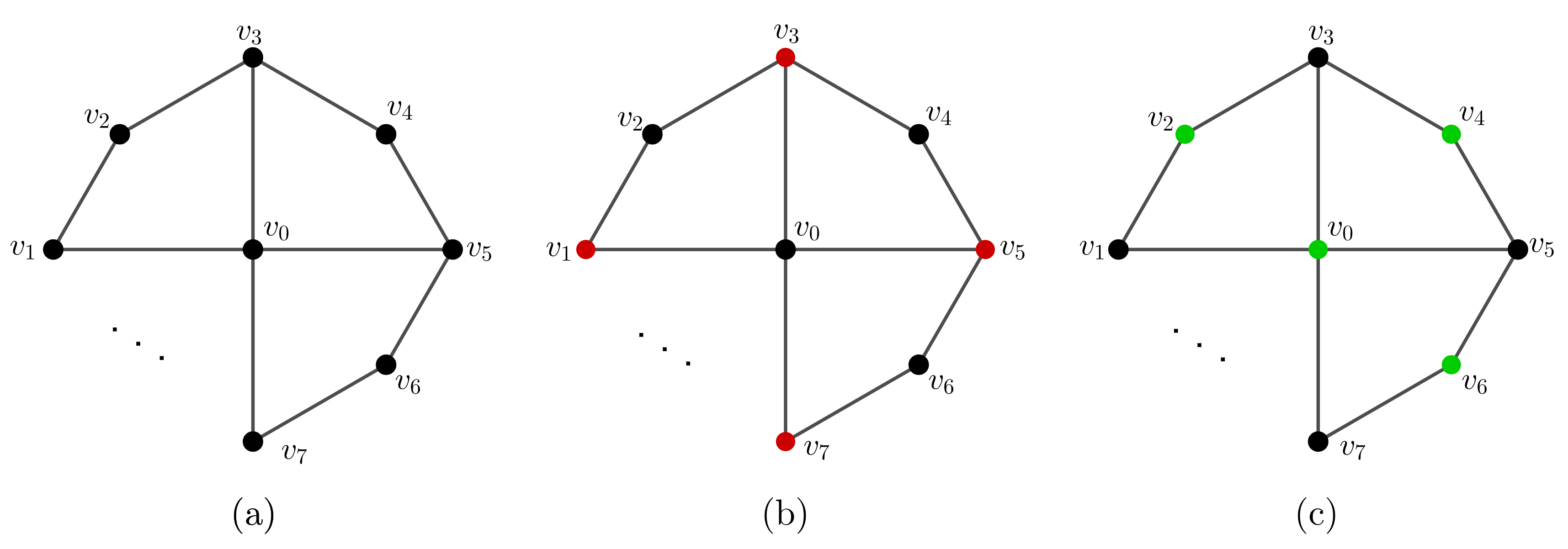
Figure 3: The vertex cover instance used in proof of Theorem 14.

Proof.

Consider the following instance: the graph as $2n+1$ vertices $v_{0},\ldots,v_{2n}$ with vertices $v_{1},\ldots,v_{2n}$ forming cycle and vertex $v_{0}$ connected to each of $v_{1},v_{3},\ldots,v_{2n-1}$ (Figure 3(a)).

The optimal vertex cover is $\{v_{1},v_{3},\ldots,2n-1\}$ (Figure 3(b)), and it is the only vertex cover of size $n$. Therefore, any other vertex cover is at best a $\frac{n+1}{n}$-approximation. When $n=9$, this is $9/8$.

We show that this vertex cover is a $9/8$-approximation for MSVC when $n=8$. Irrespective of the other in which vertices in this cover are selected, there will be $3$ edges covered at each step. Therefore, the total cover time of the edges is $3\times(1+\ldots+n)=\frac{3}{2}n(n+1)$ When $n=8$, this is $108$.

However, if we instead use the cover $(v_{0},v_{1},v_{3},\ldots,v_{2n-1})$ (Figure 3(c)) in this order, $n$ edges are covered at the first step, and $2$ edges are covered in each subsequent step, resulting in a total time of $n+2(2+\ldots+(n+1))=n(n+4)$. When $n=8$, this is $96$; but $\frac{108}{96}=\frac{9}{8}$. ∎

Theorem 15.

There exists an instance of the job times minimization problem where no solution is better than $1.13$-simultaneous approximate for even $L_{1}$ and $L_{\infty}$ norms (i.e., average completion time and makespan)

Proof.

There are two machines and three jobs. Let $\mu,\delta\in[0,1)$ be parameters we fix later. Jobs $1,2$ both have processing time $1$ on machine $1$ and processing time $1+\delta$ on machine $2$. Job $3$ has processing time $1+\mu$ on the first machine and $2$ on the second machine.

Consider possible solutions. When jobs $1,2$ are on different machines, then the best way (for both makespan and total completion time) to place job $3$ is on machine $1$. The makespan for this solution is $2+\mu$, and the total completion time is $1+(2+\mu)+(1+\delta)=4+\mu+\delta$:

$$MS_{1}=2+\mu,\quad CT_{1}=4+\mu+\delta.$$

Suppose jobs $1,2$ are both on machine $1$ now. The best way (for both makespan and total completion time) to place job $3$ is on machine $2$. The makespan and completion time are

$$MS_{2}=2,\quad CT_{2}=5.$$

Suppose jobs $1,2$ are both on machine $2$. The best solution is to place job $3$ is on machine $1$. The makespan and completion time are:

$$MS_{3}=2(1+\delta),\quad CT_{3}=3(1+\delta)+(1+\mu)=4+\mu+3\delta.$$

Therefore, the second solution has optimal makespan $2$ and when $\mu+\delta\leq 1$, the first solution has the optimal completion time. The simultaneous approximation ratio of the first solution is $\frac{2+\mu}{2}$. The simultaneous approximation ratio of the second solution is $\frac{5}{4+\mu+\delta}$. The simultaneous approximation ratio of the third solution is $\max\left(1+\delta,\frac{4+\mu+3\delta}{4+\mu+\delta}\right)$. The best possible simultaneous approximation ratio then is

$$\min\left(\frac{2+\mu}{2},\frac{5}{4+\mu+\delta},\max\left(1+\delta,\frac{4+\mu+3\delta}{4+\mu+\delta}\right)\right).$$

Optimizing this over all $\mu,\delta$ such that $0\leq\mu,\delta$ and $\mu+\delta\leq 1$, we get the value $\frac{\sqrt{61}-1}{6}>1.13$ at $(\mu,\delta)=\left(\frac{\sqrt{61}-7}{3},\frac{\sqrt{61}-7}{6}\right)$. ∎

Appendix D Identical machines

In this section, we consider machine load minimization on identical machines, so that $p_{i,j}=p_{j}$ for all jobs $j\in[n]$ and machines $i\in[m]$; that is, each job has a fixed processing time $p_{j}$. The well-known greedy algorithm places these jobs one-by-one on the machine with minimum load at that instant, until all jobs have been scheduled. [25] showed that this is a $2$-approximation algorithm for the makespan minimization problem. We observe that this is true for all ordered norms:

Observation 3.

The greedy algorithm is a simultaneous $2$-approximation for machine load minimization on identical machines.

Proof.

We prove that this greedy schedule is a $2$-approximation for all top-$k$ vectors $\mathbf{1}_{k},k\in[m]$. From Observation 1, this implies that the greedy schedule is a $2$-approximation for all norms.

Fix $k\in[d]$, and let the value of the corresponding optimal solution be $\mathrm{OPT}_{k}$. Relabel the machines $i\in[m]$ by their final loads $x_{i},i\in[m]$ in the greedy schedule so that $x_{1}\geq\ldots\geq x_{m}$. Let $\mathrm{ALG}_{k}=x_{1}+\ldots+x_{k}$ denote the objective value of the greedy algorithm. For each machine $i$, let $q_{i}$ denote the load of the last job scheduled on the machine. One natural lower bound on $\mathrm{OPT}_{k}$ is the load of any $k$ jobs, and in particular

$$\mathrm{OPT}_{k}\geq q_{1}+\ldots+q_{k}.$$

Another lower bound on $\mathrm{OPT}_{k}$ is a $k/m$ fraction of the total processing time $P=\sum_{j\in[n]}p_{j}$. But $P\geq kx_{m}$, since $x_{n}$ is the machine with least load in the final greedy schedule. Therefore,

$$\mathrm{OPT}_{k}\geq kt_{m}.$$

Fix $i\in[k]$. In the iteration job $q_{i}$ was scheduled, the load on machine $i$ was $x_{i}-q_{i}$, and let the load on machine $m$ in this iteration be denoted $x_{m}^{\prime}$. Then, since this job was scheduled on machine $i$ and not machine $m$, we must have

$$x_{i}-q_{i}\leq x_{m}^{\prime}\leq x_{m}.$$

Combine these inequalities:

$$\mathrm{ALG}_{k}=\sum_{i\in[k]}x_{i}\leq\sum_{i\in[k]}(q_{i}+x_{m})=kx_{m}+\sum_{i\in[k]}q_{i}\leq\mathrm{OPT}_{k}+\mathrm{OPT}_{k}=2\mathrm{OPT}_{k}.$$

∎

When the greedy algorithm first sorts the jobs in decreasing order of their processing times (i.e., the job with largest processing is scheduled first), its approximation ratio for makespan minimization improves to $4/3$ [cite]. We will show that it is a $3/2$-approximation for all norms:

Theorem 16.

The greedy algorithm is a simultaneous $3/2$-approximation for machine load minimization on identical machines.

We begin with a lemma:

Lemma 9.

Suppose we are given an instance with $m+r$ jobs with processing times $p_{1}\geq\ldots\geq p_{m+r}$. Let $s\in[m]$ with $s\geq r$. Then, any schedule that assigns $p_{1},\ldots,p_{m}$ to distinct machines is a $3/2$-approximation for the top-$s$ objective.

Proof.

Let $\mathrm{OPT}_{s}$ denote the optimal value for the top-$s$ objective for this instance. Since jobs $p_{1},\ldots,p_{s}$ must all be assigned to some machine, we have $\mathrm{OPT}_{s}\geq p_{1}+\ldots+p_{s}$. Further, any feasible schedule must have some $r$ machines that have at least $2r$ jobs assigned to them in total, and therefore $\mathrm{OPT}_{s}$ is lower bounded by the processing time of the smallest $s+r$ jobs, i.e., $\mathrm{OPT}_{s}\geq(p_{m-s+1}+\ldots+p_{m})+(p_{m+1}+\ldots+p_{m+r})$. Since $p_{1}\geq\ldots\geq p_{m+r}$, this implies

$$\mathrm{OPT}_{s}\geq\frac{s+r}{r}\left(p_{m+1}+\ldots+p_{m+r}\right)\geq 2\left(p_{m+1}+\ldots+p_{m+r}\right).$$

Finally, any schedule that assigns $p_{1},\ldots,p_{m}$ to distinct machines has objective value at most $(p_{1}+\ldots+p_{s})+(p_{m+1}+\ldots+p_{m+r})$. By the above inequalities, this is upper bounded by $\mathrm{OPT}_{s}+\frac{r}{r+s}\mathrm{OPT}_{s}\leq\frac{3}{2}\mathrm{OPT}_{s}$. ∎

We are ready to prove our main theorem:

Proof of Theorem 16.

We prove that the greedy algorithm is a $3/2$-approximation for all top-$k$ vectors $\mathbf{1}_{k},k\in[m]$. From Observation 1, this implies the theorem statement.

Fix $k\in[m]$, and let the value of the optimal solution be denoted $\mathrm{OPT}_{k}$, with the load on machines denoted $(x^{\mathrm{OPT}})_{1}^{\downarrow},\ldots,(x^{\mathrm{OPT}})_{m}^{\downarrow}$, so that $\mathrm{OPT}_{k}=\sum_{i\in[k]}(x^{\mathrm{OPT}})_{i}^{\downarrow}$. Relabel the machines $i\in[m]$ by their final loads $x_{i},i\in[m]$ in the greedy schedule so that $x_{1}\geq\ldots\geq x_{m}$. Denote $\mathrm{ALG}_{k}=\sum_{i\in[k]}x_{i}$ as the objective value of the greedy algorithm.

Consider the number of jobs assigned to machines $i\in[k]$ in the greedy schedule. Let $s\in[0,k]$ be the unique index such that machines $1,\ldots,s$ have at most two jobs assigned to them in the greedy schedule and machine $s+1$ has at least three jobs (if each machine $i\in[k]$ has at most two jobs assigned, set $s=k$). Denote the total load on the $s$ most loaded machines in the optimal solution by $\mathrm{OPT}_{k}^{s}=\sum_{i\in[s]}(x^{\mathrm{OPT}})_{i}^{\downarrow}$. We will bound the total load on machines $[s]$ in terms of $\mathrm{OPT}_{k}^{s}$ using Lemma 9 and the total load on machines $[s+1,k]$ in terms of $\mathrm{OPT}_{k}$.

For machines $i\in[s]$, consider the restricted instance consisting of the $m$ longest jobs $p_{1},\ldots,p_{m}$ and the other jobs assigned to the first $s$ machines $1,\ldots,s$. The greedy algorithm assigns $p_{1},\ldots,p_{m}$ to distinct machines, and since there are at most two jobs on machines $i\in[s]$, Lemma 9 implies that $x_{1}+\ldots+x_{s}$ is at most $3/2$ times the top-$s$ optimal for this restricted instance, which is at most $(3/2)\times\mathrm{OPT}_{k}^{s}$, i.e.,

$$\sum_{i\in[s]}x_{i}\leq\frac{3}{2}\mathrm{OPT}_{k}^{s}.$$ (13)

For each machine $i\in[m]$, let $q_{i}$ denote the load of the last job scheduled on the machine. Fix $i\in[k]$. At the instant job $q_{i}$ was scheduled, the load on machine $i$ was $x_{i}-q_{i}$, and let the load on machine $m$ at this instant be denoted $x_{m}^{\prime}$. Then, since this job was scheduled on machine $i$ and not machine $m$, we must have

$$x_{i}-q_{i}\leq x_{m}^{\prime}\leq x_{m}$$ (14)

Notice that since machine $s+1$ has at least three jobs assigned to it and since $q_{s+1}$ is the smallest job assigned to machine $s+1$, we have $q_{s+1}\leq\frac{1}{3}t_{s+1}$ and therefore from inequality (14) we get $x_{s+1}\leq\frac{3}{2}t_{m}$. Since $x_{s+1}\geq\ldots\geq x_{k}$, we get $x_{s+1}+\ldots+x_{k}\leq\frac{3}{2}(k-s)x_{m}$.

Let $P=\sum_{j\in[n]}p_{j}$ be the total processing time of all jobs. Since $x_{1}\geq\ldots\geq x_{m}$, we get $x_{m}\leq\frac{P-(x_{1}+\ldots+x_{s})}{m-s}$. Therefore,

$$\mathrm{ALG}_{k}=\sum_{i\in[s]}x_{i}+\sum_{i\in[s+1,k]}x_{i}\leq\sum_{i\in[s]}x_{i}+\frac{3(k-s)}{2(m-s)}\left(P-\sum_{i\in[s]}x_{i}\right)=\left(1-\frac{3(k-s)}{2(m-s)}\right)\sum_{i\in[s]}x_{i}+\frac{3(k-s)}{2(m-s)}P.$$ (15)

We can now use the bound (13) on $\sum_{i\in[s]}x_{i}$ and upper bound $P$ by $\frac{m}{k}\mathrm{OPT}_{k}$. However, this leads to a very poor bound on $\frac{\mathrm{ALG}_{k}}{\mathrm{OPT}_{k}}$ for small $k$ in the worst case. To remedy this, we need a tighter bound on $P$ in terms of $\mathrm{OPT}_{k}^{s}$ and $\mathrm{OPT}_{k}$. Using the fact that $(x^{\mathrm{OPT}})_{1}^{\downarrow}\geq\ldots\geq(x^{\mathrm{OPT}})_{m}^{\downarrow}$, we get

$$(x^{\mathrm{OPT}})_{k+1}^{\downarrow}+\ldots+(x^{\mathrm{OPT}})_{m}^{\downarrow}\leq(m-k)(x^{\mathrm{OPT}})_{k}^{\downarrow}\leq\frac{m-k}{k-s}\left((x^{\mathrm{OPT}})_{s+1}^{\downarrow}+\ldots+(x^{\mathrm{OPT}})_{k}^{\downarrow}\right)=\frac{m-k}{k-s}\left(\mathrm{OPT}_{k}-\mathrm{OPT}_{k}^{s}\right).$$

Since $P=(x^{\mathrm{OPT}})_{1}^{\downarrow}+\ldots+(x^{\mathrm{OPT}})_{m}^{\downarrow}$, this implies

$$P\leq\mathrm{OPT}_{k}^{s}+(\mathrm{OPT}_{k}-\mathrm{OPT}_{k}^{s})+\frac{m-k}{s-k}\left(\mathrm{OPT}_{k}-\mathrm{OPT}_{k}^{s}\right)=\mathrm{OPT}_{k}^{s}+\frac{m-s}{k-s}\left(\mathrm{OPT}_{k}-\mathrm{OPT}_{k}^{s}\right).$$

Combining this with (15), we get

$$\frac{\mathrm{ALG}_{k}}{\mathrm{OPT}_{k}}\leq\left(1-\frac{3(k-s)}{2(m-s)}\right)\frac{\sum_{i\in[s]}x_{i}}{\mathrm{OPT}_{k}}+\frac{3(k-s)}{2(m-s)}\left(\frac{\mathrm{OPT}_{k}^{s}}{\mathrm{OPT}_{k}}+\frac{m-s}{k-s}\left(1-\frac{\mathrm{OPT}_{k}^{s}}{\mathrm{OPT}_{k}}\right)\right)$$

Case 1: If $1-\frac{3}{2}\frac{k-s}{m-s}<0$, then we get the bound

$$\frac{\mathrm{ALG}_{k}}{\mathrm{OPT}_{k}}\leq\frac{3}{2}-\frac{3}{2}\left(1-\frac{k-s}{m-s}\right)\frac{\mathrm{OPT}_{k}^{s}}{\mathrm{OPT}_{k}}=\frac{3}{2}-\frac{3}{2}\left(\frac{m-k}{m-s}\right)\frac{\mathrm{OPT}_{k}^{s}}{\mathrm{OPT}_{k}}\leq\frac{3}{2}.$$

Case 2: If $1-\frac{3}{2}\frac{k-s}{m-s}\geq 0$, then using (13) we get

$$\frac{\mathrm{ALG}_{k}}{\mathrm{OPT}_{k}} \leq\frac{3}{2}\left(1-\frac{3(k-s)}{2(m-s)}\right)\frac{\mathrm{OPT}_{k}^{s}}{\mathrm{OPT}_{k}}+\frac{3(k-s)}{2(m-s)}\left(\frac{\mathrm{OPT}_{k}^{s}}{\mathrm{OPT}_{k}}+\frac{m-s}{k-s}\left(1-\frac{\mathrm{OPT}_{k}^{s}}{\mathrm{OPT}_{k}}\right)\right)$$

$$\leq\frac{3}{2}-\frac{3(k-s)}{4(m-s)}\frac{\mathrm{OPT}_{k}^{s}}{\mathrm{OPT}_{k}}\leq\frac{3}{2}.$$

∎

Appendix E Proof of Lemma 3

We show that a variation of [38] classical $2$-approximation algorithm for the assignment problem also works for the partial scheduling problem with $\alpha=2$. Given processing times $p$ and budget $B\geq 0$, consider the following linear programming relaxation of the problem:

$$\max \sum_{i,j}x_{i,j}$$ s.t. (LP-PS)

$$\sum_{j}p_{i,j}x_{i,j} \leq B \forall\>i\in[m],$$ (16)

$$\sum_{i}x_{i,j} \leq 1 \forall\>j\in[n],$$ (17)

$$x_{i,j} =0 \text{if}\>p_{i,j}>B\>\forall\>i,j,$$ (18)

$$x \geq 0.$$

Variable $x_{i,j}$ indicates whether or not job $j$ has been assigned to machine $i$. The objective is to maximize the number of jobs scheduled under the constraint that the makespan is at most $B$. However, to ensure that the optimal solution does not schedule a cheap job multiple times, we include constraints (17). Further, job $j$ should not be scheduled on machine $i$ if $p_{i,j}$ exceeds the makespan $B$ (constraints (18)). The optimal solution $\mathrm{OPT}$ to the partial scheduling problem clearly satisfies these constraints, and therefore $\mathrm{OPT}\leq\sum_{i,j}x^{*}_{i,j}$ for the (fractional) optimal solution $x^{*}$ to the LP.

We will round $x^{*}$ to an integral solution $x$ with makespan $\leq 2B$ and $\sum_{i,j}x_{i,j}\geq\sum_{i,j}x^{*}_{i,j}$ implying that $x$ schedules at least as many jobs as $\mathrm{OPT}$, thus completing the proof.

Let $k_{i}=\lceil\sum_{j}x^{*}_{i,j}\rceil$ for all $i$. We will construct an undirected bipartite graph $G$ with $n+k_{1}+\ldots+k_{m}$ vertices: $n$ vertices correspond to jobs and $k_{i}$ vertices correspond to machine $i$ for all $i$.

For machine $i$, let $J_{i}=\{j:x^{*}_{i,j}>0\}$ be the set of jobs (fractionally) assigned to $i$ under $x^{*}$, and relabel them so that $J_{i}=\{1,2,\ldots,l\}$; assume without loss of generality that $p_{i,1}\geq\ldots\geq p_{i,l}$. Let $v_{1},\ldots,v_{k_{i}}$ be the vertices corresponding to machine $i$. Start assigning weights $x^{*}_{i,1},x^{*}_{i,2},\ldots$ to edges $v_{1}1,v_{1}2,\ldots$, until we reach a job $a$ such that $x^{*}_{i,1}+x^{*}_{i,2}+\ldots+x^{*}_{i,a}>1$. Assign weight $1-\sum_{b\leq a-1}x^{*}_{i,b}$, i.e., just enough weight that makes the total weight of edges incident to $v_{1}$ exactly $1$. The remaining weight for job $a$, $\sum_{b\leq a}x^{*}_{i,b}-1$ goes to edge $v_{2}a$. Continue this process with job $a+1$ on vertex $v_{2}$, and so on. Since $\sum_{j\in J_{i}}x^{*}_{i,j}\leq k_{i}$, weight $x^{*}_{i,l}$ is assigned to edge $v_{k_{1}}l$. Notice that for each of $v_{1},\ldots,v_{k_{i}}$, the sum of weights of edges incident on it is at most $1$. Do this for all vertices to get $G$, and denote the weights in $G$ by $w$

By construction, the sum of weights of edges incident on a vertex is at most $1$ if it corresponds to a machine. From constraints (17) and the construction, the sum of weights of edges incident on vertices corresponding to jobs is also at most $1$. Therefore, $w$ forms a fractional matching on $G$. Further, the sum of all edge weights, $\|w\|_{1}$, is $\sum_{i,j}x^{*}_{i,j}$. Since $G$ is bipartite, this fractional matching can be rounded to a integral matching $y$ at least as large as $w$, i.e., $\|y\|_{1}\geq\|w\|_{1}$. Obtain integral solution $x$ by assigning jobs to machines according to matching $y$, i.e., if job $j$ is adjacent to a vertex corresponding to machine $i$, assign $x_{i,j}=1$; assign $x_{i,j}=0$ in all other cases. Then we have that $\sum_{i,j}x_{i,j}=\|y_{1}\|\geq\|w_{1}\|=\sum_{i,j}x^{*}_{i,j}$.

It remains to argue that the makespan to each machine is at most $2B$. Fix machine $i$. Suppose jobs $j_{1},\ldots,j_{k_{i}}$ are adjacent to vertices $v_{1},\ldots,v_{k_{i}}$ respectively in matching $y$. Then, since jobs were sorted in decreasing order, the processing time $p_{i,j_{2}}$ is upper bounded by the processing time of jobs adjacent to $v_{1}$ in $x^{*}$:

$$p_{i,j_{2}}=p_{i,j_{2}}\sum_{j:w(v_{1}j)>0}w(v_{1},j)\leq\sum_{j:w(v_{1}j)>0}p_{i,j}w(v_{1},j).$$

Similarly, for each $b\in[2,j_{k_{i}}]$, we get $p_{i,j_{b}}\leq\sum_{j:w(v_{b-1,j})>0}p_{i,j}w(v_{b-1},j)$.

Adding these,

$$\sum_{a\in[2,k_{i}]}p_{i,j_{a}}\leq\sum_{a\in[2,k_{i}]}\sum_{j:w(v_{b-1,j})>0}p_{i,j}w(v_{b-1},j)\leq\sum_{j\in J_{i}}p_{i,j}x^{*}_{i,j}\leq B.$$

Since $p_{i,j_{1}}\leq B$ by constraint (16), we get the total makespan on machine $i$ under $x$ is

$$p_{i,j_{1}}+\sum_{a\in[2,k_{i}]}p_{i,j_{a}}\leq 2B.$$

Appendix F Matroids and the greedy algorithm

Suppose we are give a matroid $\mathcal{M}=(X,\mathcal{I})$ along with non-negative costs $c:X\to\mathbb{R}_{\geq 0}$ for matroid elements. The cost of a base $B$ is defined as the sum of costs of elements of $B$. The greedy algorithm to produce a minimum-cost base maintains a set $S\subseteq X$, initially set as $\emptyset$, and iteratively adds a minimum-cost element from $X\setminus S$ to $S$ until $S$ is a base. It is well-known that the greedy algorithm produces is optimal for matroids. Consider the more general problem: for a base $B\subseteq X$, define the cost vector $C_{B}\in\mathbb{R}^{|X|}$ as:

$$C_{B}(x)=\begin{cases}c(x)&\text{if}\>x\in X,\\ 0&\text{otherwise}.\end{cases}$$

Given a weight vector $w\in\mathbf{W}_{|X|}$, consider the problem of minimizing an arbitrary monotonic symmetric norm $\|\cdot\|$ of $C_{B}$ across all bases $B$:

$$\min_{B\text{ is a base}}\|C_{B}\|$$

$\|C_{B}\|_{\mathbf{1}_{|X|}}$ is $\sum_{x\in B}c(x)$, i.e., the classical cost of $B$. We show that the greedy algorithm is actually optimal for symmetric monotonic norms:

Observation 4.

The greedy algorithm is simultaneously optimal with respect to all monotonic symmetric norms.

Proof.

Fix an arbitrary symmetric norm $\|\cdot\|$. By induction, we show that the set $S$ is a subset of some minimum norm base throughout the algorithm. This is clearly true initially when $S=\emptyset$. Suppose it is true at the beginning of some iteration so that $S\subseteq B$, and suppose that the greedy algorithm adds $x\in X$ to $S$ in this iteration. If $S\cup\{x\}\in B$, we are done. Otherwise, we can extend $S$ to a base $B^{\prime}$ such that $|B^{\prime}\setminus B|=|B\setminus B^{\prime}|=1$. Suppose $B\setminus B^{\prime}=\{y\}$. By definition of the greedy algorithm, we must have $c(y)\geq c(x)$, implying $C_{B^{\prime}}\preceq C_{B}$. Therefore, by Lemma 1, we have that $\|C_{B^{\prime}}\|\leq\|C_{B}\|$. This completes the induction step, and the proof. ∎

Corollary 17.

Kruskal’s algorithm produces a spanning tree that is simultaneously optimal for all monotonic symmetric norms.

Appendix G Submodular base polytopes

The main result of this section is the following:

Observation 5.

Given any submodular set function $f:2^{[n]}\to\mathbb{R}_{\geq 0}$ and the corresponding submodular base polytope $B(f)$, the minimum norm point $x^{*}$ is also minimum with respect to all symmetric monotonic norms $\|\cdot\|$, i.e., $x^{*}=\arg\min_{x\in B(f)}\|x\|$.

We will use the following result from [7] that characterizes majorization:

Lemma 10 ([7] Theorem II.1.10).

$x\preceq y$ if and only if $x$ is in the convex hull of all vectors obtained by permuting the coordinates of $y$.

Proof of Observation 5.

Partition $[n]$ into nonempty sets $F_{1},\ldots,F_{k}$ such that $x^{*}_{i}=t_{j}$ whenever $i\in F_{j}$, and $t_{1}>t_{2}>\ldots>t_{k}$. That is, the sets $F_{1},\ldots,F_{k}$ partition the index set $[n]$ by the coordinate values of $x^{*}$ in a decreasing order.

Theorem 4 in [26] asserts that $x^{*}$ satisfies

$$f\left(F_{j}\cup\ldots\cup F_{k}\right)=x^{*}\left(F_{j}\cup\ldots\cup F_{k}\right)\quad\forall\>j\in[k].$$ (19)

Consider some $x\in B(f)$, and denote $x-x^{*}=\epsilon$. We will show that $x^{*}\preceq x$, and so $\|x^{*}\|\leq\|x\|$ for all norms $\|\cdot\|$ by Lemma 1, implying the theorem.

Note that since $x\in B(f)$, $x([n])=x^{*}([n])=f([n])$ and therefore $\epsilon([n])=0$. Also, since $x\in B(f)$, we have $x(F_{j+1}\cup\ldots\cup F_{k})\leq f(F_{j+1}\cup\ldots\cup F_{k})$ for all $j\in[k]$. Together with (19), these facts imply that

$$\epsilon(F_{1}\cup\ldots\cup F_{j})\geq 0\quad\forall\>j\in[k].$$ (20)

Consider $\overline{x}\in\mathbb{R}^{n}$ defined as $\overline{x}_{i}=t_{j}+\frac{\epsilon(F_{j})}{|F_{j}|}$ for all $i\in F_{j},j\in[k]$. We will show that $\overline{x}\preceq x$ and $x^{*}\preceq\overline{x}$, implying that $x^{*}\preceq x$ and finishing the proof.

Notice that for such $i,j$ we have $|F_{j}|\overline{x}_{i}=|F_{j}|t_{j}+\epsilon(F_{j})=x^{*}(F_{j})+\epsilon(F_{j})=x(F_{j})$. That is, $\overline{x}_{i}=x(F_{j})/|F_{j}|$ for all $i\in F_{j}$. Lemma 10 then implies that $\overline{x}\preceq x$.

Finally, we show that $x^{*}\preceq\overline{x}$ by a direct computation. Given $i\in[d]$, let $j\in[k]$ be the unique index such that $i=|F_{1}|+\ldots+|F_{j-1}|+s$ for $s\in[|F_{j}|]$. Then, since $t_{1}>\ldots>t_{k}$, we have

$$\sum_{p\in[i]}(x^{*})_{p}^{\downarrow}=\sum_{l\in[j-1]}|F_{l}|t_{l}+st_{j}.$$

Therefore,

$$\sum_{p\in[i]}\overline{x}_{p}^{\downarrow}-\sum_{p\in[i]}(x^{*}_{p})^{\downarrow}$$

$$\geq \sum_{p\in[i]}\overline{x}_{p}-\sum_{p\in[i]}(x^{*}_{p})^{\downarrow}$$

$$= \left(s\left(t_{j}+\frac{\epsilon(F_{j})}{|F_{j}|}\right)+\sum_{l\in[j-1]}|F_{l}|\left(t_{l}+\frac{\epsilon(F_{l})}{|F_{l}|}\right)\right)-\left(st_{j}+\sum_{l\in[j-1]}|F_{l}|t_{l}\right) \left(\text{definition}\right)$$

$$= \frac{s}{|F_{j}|}\epsilon(F_{j})+\sum_{l\in[j-1]}\epsilon(F_{l})$$

$$= \frac{s}{|F_{j}|}\left(\sum_{l\in[j]}\epsilon(F_{l})\right)+\left(1-\frac{s}{|F_{j}|}\right)\left(\sum_{l\in[j-1]}\epsilon(F_{l})\right)\geq 0 \left(\text{equation }(\ref{eqn: submodular-mnp-error-is-nonnegative})\text{ and }s\in[|F_{j}|]\right).$$

∎

References

- [1] Mohsen Abbasi, Aditya Bhaskara, and Suresh Venkatasubramanian. Fair Clustering via Equitable Group Representations. In Proceedings of the 2021 ACM Conference on Fairness, Accountability, and Transparency, FAccT ’21, pages 504–514, New York, NY, USA, March 2021. Association for Computing Machinery.
- [2] Yossi Azar and Amir Epstein. Convex programming for scheduling unrelated parallel machines. In Proceedings of the thirty-seventh annual ACM symposium on Theory of computing, STOC ’05, pages 331–337, New York, NY, USA, May 2005. Association for Computing Machinery.
- [3] Yossi Azar and Shai Taub. All-Norm Approximation for Scheduling on Identical Machines. In Torben Hagerup and Jyrki Katajainen, editors, Algorithm Theory - SWAT 2004, Lecture Notes in Computer Science, pages 298–310, Berlin, Heidelberg, 2004. Springer.
- [4] Nikhil Bansal, Jatin Batra, Majid Farhadi, and Prasad Tetali. Improved Approximations for Min Sum Vertex Cover and Generalized Min Sum Set Cover. In Proceedings of the 2021 ACM-SIAM Symposium on Discrete Algorithms (SODA), Proceedings, pages 998–1005. Society for Industrial and Applied Mathematics, January 2021.
- [5] Nikhil Bansal and Kirk Pruhs. Server scheduling in the Lp norm: a rising tide lifts all boat. In Proceedings of the thirty-fifth annual ACM symposium on Theory of computing, STOC ’03, pages 242–250, New York, NY, USA, June 2003. Association for Computing Machinery.
- [6] Solon Barocas, Moritz Hardt, and Arvind Narayanan. Fairness and Machine Learning: Limitations and Opportunities. fairmlbook.org, 2019.
- [7] Rajendra Bhatia. Matrix Analysis. Springer Science & Business Media, December 2013. Google-Books-ID: lh4BCAAAQBAJ.
- [8] Avrim Blum, Prasad Chalasani, Don Coppersmith, Bill Pulleyblank, Prabhakar Raghavan, and Madhu Sudan. The minimum latency problem. In Proceedings of the twenty-sixth annual ACM symposium on Theory of computing - STOC ’94, pages 163–171, Montreal, Quebec, Canada, 1994. ACM Press.
- [9] Chloe Courtney Bohl. Boston moving toward giving residents voice in ‘participatory budgeting’, December 2022.
- [10] Jaroslaw Byrka, Krzysztof Sornat, and Joachim Spoerhase. Constant-factor approximation for ordered k-median | Proceedings of the 50th Annual ACM SIGACT Symposium on Theory of Computing. STOC 2018: Proceedings of the 50th Annual ACM SIGACT Symposium on Theory of Computing, 2018.
- [11] Deeparnab Chakrabarty and Chaitanya Swamy. Interpolating between k-Median and k-Center: Approximation Algorithms for Ordered k-Median. In 45th International Colloquium on Automata, Languages, and Programming (ICALP 2018), volume 107 of Leibniz International Proceedings in Informatics (LIPIcs), pages 29:1–29:14, Dagstuhl, Germany, 2018. ISSN: 1868-8969.
- [12] Deeparnab Chakrabarty and Chaitanya Swamy. Approximation algorithms for minimum norm and ordered optimization problems. In Proceedings of the 51st Annual ACM SIGACT Symposium on Theory of Computing, STOC 2019, pages 126–137, New York, NY, USA, June 2019. Association for Computing Machinery.
- [13] Deeparnab Chakrabarty and Chaitanya Swamy. Simpler and Better Algorithms for Minimum-Norm Load Balancing. In 27th Annual European Symposium on Algorithms (ESA 2019), volume 144 of Leibniz International Proceedings in Informatics (LIPIcs), pages 27:1–27:12, Dagstuhl, Germany, 2019. ISSN: 1868-8969.
- [14] Ashok K. Chandra and C. K. Wong. Worst-Case Analysis of a Placement Algorithm Related to Storage Allocation. SIAM Journal on Computing, 4(3):249–263, September 1975. Publisher: Society for Industrial and Applied Mathematics.
- [15] Moses Charikar, Samir Khuller, David M. Mount, and Gin Narasimhan. Algorithms for facility location problems with outliers: 2001 Operating Section Proceedings, American Gas Association. Proceedings of the 12th Annual ACM-SIAM Symposium on Discrete Algorithms, pages 642–651, 2001.
- [16] Eden Chlamtac, Yury Makarychev, and Ali Vakilian. Approximating Fair Clustering with Cascaded Norm Objectives. In Proceedings of the 2022 Annual ACM-SIAM Symposium on Discrete Algorithms (SODA), Proceedings, pages 2664–2683. Society for Industrial and Applied Mathematics, January 2022.
- [17] Zhen Dai, Yury Makarychev, and Ali Vakilian. Fair Representation Clustering with Several Protected Classes | Proceedings of the 2022 ACM Conference on Fairness, Accountability, and Transparency. Proceedings of the 2022 ACM Conference on Fairness, Accountability, and Transparency, 2022.
- [18] Majid Farhadi, Alejandro Toriello, and Prasad Tetali. The Traveling Firefighter Problem. In Proceedings of the 2021 SIAM Conference on Applied and Computational Discrete Algorithms (ACDA21), Proceedings, pages 205–216. Society for Industrial and Applied Mathematics, January 2021.
- [19] Samuel Freeman. Original Position. In Edward N. Zalta, editor, The Stanford Encyclopedia of Philosophy. Metaphysics Research Lab, Stanford University, summer 2019 edition, 2019.
- [20] Yingqiang Ge, Shuya Zhao, Honglu Zhou, Changhua Pei, Fei Sun, Wenwu Ou, and Yongfeng Zhang. Understanding Echo Chambers in E-commerce Recommender Systems. In Proceedings of the 43rd International ACM SIGIR Conference on Research and Development in Information Retrieval, SIGIR ’20, pages 2261–2270, New York, NY, USA, July 2020.
- [21] Mehrdad Ghadiri, Mohit Singh, and Santosh S. Vempala. Constant-Factor Approximation Algorithms for Socially Fair $k$-Clustering, June 2022. arXiv:2206.11210 [cs].
- [22] Ashish Goel and Adam Meyerson. Simultaneous Optimization via Approximate Majorization for Concave Profits or Convex Costs. Algorithmica, 44(4):301–323, April 2006.
- [23] Daniel Golovin, Anupam Gupta, Amit Kumar, and Kanat Tangwongsan. All-Norms and All-Lp-Norms Approximation Algorithms. IARCS Annual Conference on Foundations of Software Technology and Theoretical Computer Science, 2008.
- [24] R. L. Graham. Bounds for certain multiprocessing anomalies. The Bell System Technical Journal, 45(9):1563–1581, November 1966.
- [25] R. L. Graham. Bounds on Multiprocessing Timing Anomalies. SIAM Journal on Applied Mathematics, 17(2):416–429, March 1969. Publisher: Society for Industrial and Applied Mathematics.
- [26] Swati Gupta, Michel Goemans, and Patrick Jaillet. Solving Combinatorial Games using Products, Projections and Lexicographically Optimal Bases, March 2016. arXiv:1603.00522 [cs].
- [27] Swati Gupta, Akhil Jalan, Gireeja Ranade, Helen Yang, and Simon Zhuang. Too Many Fairness Metrics: Is There a Solution?, March 2020.
- [28] Swati Gupta, Jai Moondra, and Mohit Singh. Which Lp norm is the fairest? Approximations for fair facility location across all "p", May 2023. arXiv:2211.14873 [cs].
- [29] Sharat Ibrahimpur and Chaitanya Swamy. Minimum-Norm Load Balancing Is (Almost) as Easy as Minimizing Makespan. In 48th International Colloquium on Automata, Languages, and Programming (ICALP 2021), volume 198, pages 81:1–81:20, Dagstuhl, Germany, 2021. ISSN: 1868-8969.
- [30] Kamal Jain and Vijay V. Vazirani. Approximation algorithms for metric facility location and k-Median problems using the primal-dual schema and Lagrangian relaxation. Journal of the ACM, 48(2):274–296, March 2001.
- [31] Jon Kleinberg. An Impossibility Theorem for Clustering. Advances in Neural Information Processing Systems 15 (NIPS 2002), 2002.
- [32] Jon Kleinberg. Inherent Trade-Offs in Algorithmic Fairness. In Abstracts of the 2018 ACM International Conference on Measurement and Modeling of Computer Systems, SIGMETRICS ’18, page 40, New York, NY, USA, June 2018. Association for Computing Machinery.
- [33] A. Kumar and J. Kleinberg. Fairness measures for resource allocation. In Proceedings 41st Annual Symposium on Foundations of Computer Science, pages 75–85, November 2000. ISSN: 0272-5428.
- [34] V. S. Anil Kumar, Madhav V. Marathe, Srinivasan Parthasarathy, and Aravind Srinivasan. A unified approach to scheduling on unrelated parallel machines. Journal of the ACM, 56(5):28:1–28:31, August 2009.
- [35] Xiaofei Liu and Weidong Li. Approximation algorithms for the multiprocessor scheduling with submodular penalties. Optimization Letters, 15(6):2165–2180, September 2021.
- [36] Maryam Negahbani and Deeparnab Chakrabarty. Better Algorithms for Individually Fair k-Clustering. In Advances in Neural Information Processing Systems, volume 34, pages 13340–13351. Curran Associates, Inc., 2021.
- [37] Kalen Patton, Matteo Russo, and Sahil Singla. Submodular Norms with Applications To Online Facility Location and Stochastic Probing. In Approximation, Randomization, and Combinatorial Optimization. Algorithms and Techniques (APPROX/RANDOM 2023), volume 275 of Leibniz International Proceedings in Informatics (LIPIcs), pages 23:1–23:22, 2023.
- [38] David B. Shmoys and Eva Tardos. An approximation algorithm for the generalized assignment problem. Mathematical Programming, 62(1):461–474, February 1993.