An Efficient Self-Supervised Cross-View Training For Sentence Embedding

Abstract

Self-supervised sentence representation learning is the task of constructing an embedding space for sentences without relying on human annotation efforts. One straightforward approach is to finetune a pretrained language model (PLM) with a representation learning method such as contrastive learning. While this approach achieves impressive performance on larger PLMs, the performance rapidly degrades as the number of parameters decreases. In this paper, we propose a framework called Self-supervised Cross-View Training (SCT) to narrow the performance gap between large and small PLMs. To evaluate the effectiveness of SCT, we compare it to 5 baseline and state-of-the-art competitors on seven Semantic Textual Similarity (STS) benchmarks using 5 PLMs with the number of parameters ranging from 4M to 340M. The experimental results show that STC outperforms the competitors for PLMs with less than 100M parameters in 18 of 21 cases.

1 Introduction

Self-supervised sentence representation learning is the task of constructing an embedding space for sentences without relying on human annotation efforts. Recent advancements in self-supervised sentence representation present promising results on various downstream tasks such as Semantic Textual Similarity (STS) and text classification. For example, Gao et al. (2021) found that self-supervised sentence embedding methods could be on par with supervised methods Reimers and Gurevych (2019) on various STS benchmarks.

A straightforward approach to self-supervised sentence representation is to finetune a pre-trained language model (PLM), i.e., BERT Devlin et al. (2019) and RoBERTa Liu et al. (2019), with a representation learning technique. One popular method is contrastive learning. This learning method enables self-supervised representation learning by creating a self-referencing mechanism through data augmentation Gao et al. (2021); Zhang et al. (2022b); Zhou et al. (2022); Klein and Nabi (2022); Yan et al. (2021); Liu et al. (2021); Kim et al. (2021); Cao et al. (2022). These works have demonstrated improvements over existing self-supervised techniques in sentence embedding benchmark datasets (i.e., STS and text classification).

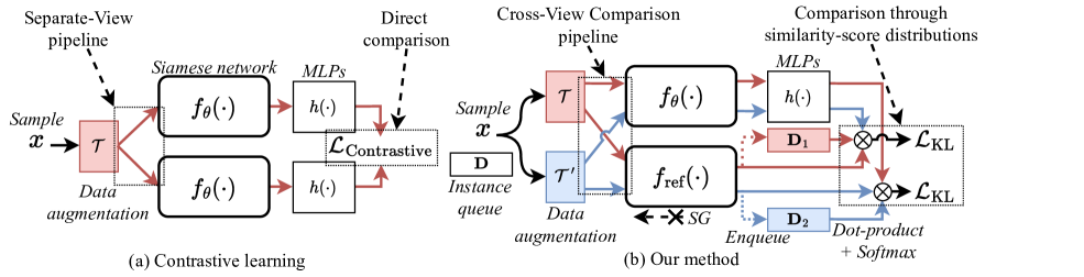
Figure 1: (a) The overview of self-supervised contrastive learning for sentence embedding. Contrastive learning is applied to directly compare the input $x$ produced from the separate-view pipeline $\mathcal{T}$. (b) The Self-Supervised Cross-View Training (SCT) pipeline. We calculate similarity score distributions between two networks ($f_{\theta}$ and $f_{\text{ref}}$) from the cross-view pipeline and minimize them through similarity-score distribution. In addition, the two networks do not require identical architecture nor share weights. They can be large and small networks (distillation) or Siamese networks.

Figure 2 shows how three existing methods SimCSE Gao et al. (2021), DiffCSE Chuang et al. (2022), and DCLR Zhou et al. (2022) perform on the BERT architecture as we varied the number of parameters from 4M to 340M. While these self-supervised techniques achieve impressive performance on larger PLMs (i.e., those with more than 100M parameters), the performance rapidly degrades as the number of parameters decreases Wu et al. (2021); Zhang et al. (2022b); Limkonchotiwat et al. (2022). The figure also shows how the data points organize themselves into two distinct groups: LL and HH.

• High Cost, High Performance (HH). As shown in Figure 2, all models in this group, i.e., BERT-Base and BERT-Large, score more than 75, with the inference times over 420.9 seconds regardless of the learning method.

• Low Cost, Low Performance (LL). This group contains all methods on models with less than 100 parameters, i.e., BERT-Tiny, BERT-Mini, and BERT-Small. All models in this group score less than 70, with the inference times less than 84.7 seconds regardless of the learning method.

Despite the apparent benefit of low computation costs, smaller models, i.e., BERT-Tiny, BERT-Mini, and BERT-Small, are often neglected. Greater emphasis should be placed on exploring the potential to enhance the performance of smaller models through novel learning methods specifically tailored to their unique characteristics.

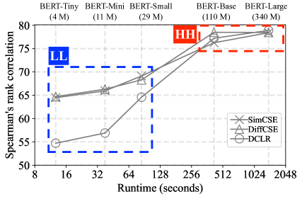
Figure 2: Comparison between sentence representation methods on different model sizes. We averaged Spearman’s rank correlation across seven STS datasets. LL denotes the low-cost, low-performance group, and HH denotes the high-cost, high-performance group.

In this paper, we propose a framework called Self-Supervised Cross-View Training (SCT) to narrow the performance gaps between large and small PLMs. Figure 1 displays the difference between the traditional contrastive learning approach and ours. As shown in Figure 1a, the two views are separated for contrastive learning, and the outputs from $h(\cdot)$ are directly compared to each other. Figure 1b highlights the key distinctions of SCT based on two concepts: cross-view comparison and similarity-score-distribution learning.

• Cross-view comparison: The ability to self-reference is crucial to self-supervised learning. We derive a novel mechanism for two different augmented views to reference each other.

• Similarity-score-distribution learning: The way we quantify loss is critical to any learning process. Our method calculates the loss by measuring the discrepancy between two similarity score distributions obtained from cross-comparing two different views.

The combination of these two concepts provides additional guidance which improves the effectiveness of self-supervised sentence representation learning on small PLMs.

To evaluate the effectiveness of SCT, we compare it to state-of-the-art (SOTA) competitors on STS, re-ranking, and natural language inference (NLI) benchmarks. We also employ a distillation setting using BERT-Large-SimCSE as a teacher model. The experimental results on STS demonstrated that our framework could address the drastic performance degradation problems in small PLMs by outperforming competitors in every case when the number of parameters is less than 100M. For the smallest model (#parameter: 4 million), we improved the performance from 64.47 to 69.73 points compared to SimCSE. In the case of large PLMs (i.e., those with more than 100M parameters), our model’s performance was on par with the current SOTA model when tested on BERT-Base and BERT-Large. For the distillation setting, we outperformed all distillation competitors on all PLMs. For the re-ranking and NLI tasks, we improved the downstream tasks’ performance for nearly all settings.

The contributions of our work are as follows:

• We formulate a cross-view comparison pipeline to provide a more robust self-referencing mechanism for self-supervised sentence representation learning on smaller PLMs (those with less than 100M parameters).

• Based on the cross-view comparison, we propose a method to measure the discrepancies between the cross-view outputs by comparing their respective similarity score distributions rather than the direct outputs.

• We evaluate the effectiveness of SCT against five competitors on three families of PLMs using STS and downstream benchmark datasets. In addition, we also provide an in-depth analysis of different components in the cross-view pipeline to assess their effectiveness individually.

2 Related Work

Self-supervised learning is becoming more popular as a method to learn sentence representation from pre-trained language models (PLMs) without annotated information from training corpora. We cover well-known self-supervised sentence representation learning techniques in the following subsections.

2.1 Contrastive Learning

Contrastive learning constructs an embedding space by treating augmentations of an anchor as positives and other samples as negatives. The anisotropic problem is addressed by pulling a positive sample and pushing a negative sample with respect to an anchor sample. Gao et al. (2021) showed that the way we obtain positive and negative samples is critical to the performance of the representation. Kim et al. (2021); Cao et al. (2022) utilized a different PLM to generate positive and negative samples for each anchor. Fang et al. (2020) derived a method using two back-translations to create two different augmented views. Another popular approach is to generate positive and negative pairs using feature dimension dropouts Gao et al. (2021); Yan et al. (2021); Liu et al. (2021); Klein and Nabi (2022). The experimental results from these works outperformed the traditional self-supervised sentence embedding methods.

A more advanced technique uses an additional function to help distinguish positive from negative samples. For example, Zhou et al. (2022) proposed an additional debias function by mapping negative samples to the Gaussian distribution while individually assigning a weight to each contrastive negative sample. Zhang et al. (2022b) proposed a virtual augmentation scheme by approximating the nearest neighborhood from the neighboring samples to create the virtual negative samples. Chuang et al. (2022) introduced a discriminator network to contrastive learning by classifying whether each word in a sentence is edited. Although these works demonstrated good performance, contrastive learning requires a judicial consideration of negative sampling to prevent false negatives.

2.2 Learning Without Negative Samples

A popular method to avoid false negatives is to design a learning process that uses only positive samples. BSL Zhang et al. (2021) adapted BYOL’s learning algorithm Grill et al. (2020), which maximizes the similarity between two augmented views of each sentence. In particular, BSL created two augmented views from a PLM. The method uses a weighted exponential moving average of embeddings as a self-referencing mechanism. Klein and Nabi (2022) adapted a redundancy representation learning algorithm from Zbontar et al. (2021) and added a cosine similarity to maximize the similarity between the two samples formulated from high and low intense feature-dropout rate models. While these methods allow us to perform self-supervised learning without negative samples, they are still outperformed by contrastive learning.

2.3 Sentence Representation Distillation

Distillation is a widely used technique for creating a small PLM (student) from an existing large PLM (teacher) Turc et al. (2019); Wang et al. (2020). Several sentence representation works proposed self-supervised distillation frameworks. For instance, Wu et al. (2021) proposed an self-supervised contrastive distillation. They formulated an anchor and other components (positives and negatives) of contrastive learning using a small and large PLMs, respectively. Limkonchotiwat et al. (2022) proposed a distillation framework based on the instance queue concept. A large PLM formulated representations for an instance queue, while the small PLM mimicked the relation between its representations and those in the instance queue.

These methods have been shown to reduce the performance gap between a small and large PLMs effectively. However, none of the sentence representation works present how to decrease the gap without utilizing a large PLM. This research question is an important problem that needs to be addressed, especially since utilizing a large PLM may not always be feasible in practice. Therefore, it is crucial to propose techniques that can decrease the gap with or without utilizing knowledge from a large PLM.

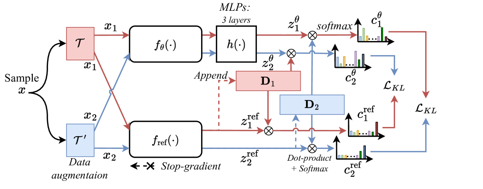
Figure 3: The overview of Self-Supervised Cross-View Training (SCT).

2.4 Learning From Distribution

A recent approach from computer vision to mitigating the false negative problem is replacing binary labels with a distribution of similarity scores. The main idea is to compare samples $a$ and $p$ using similarity scores computed from the same collection of instances $\mathbf{D}$ as soft labels. In particular, the discrepancy between $a$ and $p$ is expressed as the similarity score discrepancy. Fang et al. (2021) proposed a knowledge distillation method by training a student network to imitate the similarity score distribution formulated by a teacher network. Tejankar et al. (2021) introduced a distribution learning paradigm using a similarity distribution score inferred by a momentum encoder over a set of instances. Zheng et al. (2021) proposed a representation learning technique by modeling the relationship distribution between weak and contrastive augmentation schemes. These works’ experimental results demonstrated higher performance than contrastive learning and avoided false negatives.

2.5 Summary

As discussed in Section 2.1, the main drawback of contrastive learning is the binary distinction between positive and negative samples. Near duplicates can be mistakenly used as negative samples. While there exist learning methods that use only positive samples, they are still outperformed by contrastive learning.

Based on various experimental studies, the paradigm of learning from distribution shows promising results compared to the other two approaches. However, we have found that the direct application of distribution learning to our problem does not yield consistent performance improvement (see Table 4 in Section 5.3.1). We developed a self-referencing mechanism through data augmentation, which is needed to improve the distribution learning strategy for self-supervised sentence representation learning. Moreover, our framework also allows sentence representation learning in a distillation manner. In particular, we employ a larger model as the teacher model to let a smaller model mimics the teacher’s property.

3 Proposed Method

One of the challenges of using small models is the limited number of parameters. An empirical study has shown that larger models have enough parameters to solve complex problems with simple techniques, while smaller ones require more guidance to solve complex problems Brutzkus and Globerson (2019); Wang et al. (2020). Based on this observation, we design our proposed solution, Self-Supervised Cross-View Training (SCT), to enhance the learning guidance for smaller models (those with less than 100M parameters) by improving the self-referencing and discrepancy measurement mechanisms.

Figure 3 illustrates the SCT pipeline and highlights the two mechanisms we introduce to improve the learning guidance: cross-view comparison pipeline and similarity-score-distribution Learning. In what follows, we describe how the cross-view pipeline improves the robustness of the self-referencing mechanism in Section 3.1. Section 3.2 presents the mechanism we use to measure the discrepancies between cross-view outputs. We explain our proposed SCT loss function in Section 3.3. Finally, we introduce sentence representation distillation into our proposed framework in Section 3.4.

3.1 Cross-View Comparison Pipeline

As stated in the introduction, we devise a cross-view comparison pipeline to improve the robustness of the self-referencing mechanism. Figure 3 illustrates how the two augmented views are fed to both online (updatable) $f_{\theta}(\cdot)$ and reference (un-updatable) $f_{\text{ref}}(\cdot)$ networks and how their outputs are compared in a cross-view pattern. In this way, we use both views as references and do not compare outputs originating from the same view to each other.

Given a new sample $x$, two augmentations $\mathcal{T}$ and $\mathcal{T}^{\prime}$ are created from two different back-translations to produce two views $x_{1}=\mathcal{T}(x)$ and $x_{2}=\mathcal{T}^{\prime}(x)$. Our framework allows various data augmentation schemes, i.e., masked language model (MLM) or Synonym replacement. We found that back-translation improves the performance of downstream tasks the most, and we used them to create cross-view inputs. (see Section 5.3.3 for design analysis).

Online representations ($z^{\theta}$). The views $x_{1}$ and $x_{2}$ are first encoded by an encoder $f_{\theta}(\cdot)$ into a sentence representation, which is then mapped by the MLPs projector $h(\cdot)$ onto the representations $z^{\theta}_{1}=h(f_{\theta}(x_{1}))$ and $z^{\theta}_{2}=h(f_{\theta}(x_{2}))$.

Reference representations ($z^{\text{ref}}$). The views $x_{1}$ and $x_{2}$ are again encoded by the $f_{\text{ref}}(\cdot)$ encoder to be used as references for the next step $z^{\text{ref}}_{1}=f_{\text{ref}}(x_{1})$ and $z^{\text{ref}}_{2}=f_{\text{ref}}(x_{2})$. Note that the architecture and weights of the target network $f_{\text{ref}}(\cdot)$ and the online network $f_{\theta}(\cdot)$ are identical, and all encoder outputs are normalized.

Instance queues ($\mathbf{D}$). We denote two instance queues that are formulated from the cross-view reference representations, $z^{\text{ref}}_{1}$ and $z^{\text{ref}}_{2}$, as $\mathbf{D}_{1}=[\mathbf{d}^{\text{1}}_{1},...,\mathbf{d}^{k}_{1}]$ and $\mathbf{D}_{2}=[\mathbf{d}^{1}_{2},...,\mathbf{d}^{k}_{2}]$ where $k$ is the queue length and $\mathbf{d}$ is the sentence vector obtained from $f_{\text{ref}}$ with $\mathbf{d}^{k}_{1}=z^{\text{ref}}_{1}$ and $\mathbf{d}^{k}_{2}=z^{\text{ref}}_{2}$. These instance queues enable the dynamic construction of a large and consistent negative sample, facilitating distribution learning. Fang et al. (2021); Tejankar et al. (2021); Zheng et al. (2021). At the beginning of each minibatch, we enqueue and dequeue instance queues in a “first-in-first-out" manner.

3.2 Similarity-Score Distribution

The next step is to calculate similarity score distributions for cross-view comparison. As shown in Figure 3, we enforce the online representations $z^{\theta}_{1}$ and $z^{\theta}_{2}$ to maintain the consistency of the reference representations $z^{\text{ref}}_{2}$ and $z^{\text{ref}}_{1}$ through instance queues $\mathbf{D}_{2}$ and $\mathbf{D}_{1}$, respectively. When the online network can match the reference representation in a large number of negative samples, the online network gains robustness to unseen inputs, which is necessary for sentence embedding.

We formulate the cross-view and reference distributions as follows:

• We formulate a cross-view distribution that compares two augmented views called $c^{\theta}_{1}=\mathbf{SR}(z^{\theta}_{1},\mathbf{D}_{2},\tau^{\theta})$.

• Similarly, we derive another cross-view distribution called $c^{\theta}_{2}=\mathbf{SR}(z^{\theta}_{2},\mathbf{D}_{1},\tau^{\theta})$.

• We calculate the self-references with respect to the previous online distributions as follows: $c^{\text{ref}}_{1}=\mathbf{SR}(z^{\text{ref}}_{1},\mathbf{D}_{1},\tau^{\text{ref}})$ and $c^{\text{ref}}_{2}=\mathbf{SR}(z^{\text{ref}}_{2},\mathbf{D}_{2},\tau^{\text{ref}})$.

We define the similarity score distribution function $\mathbf{SR}(\cdot)$ as a dot product function between a sentence representation and an instance queue:

$$\mathbf{SR}\left(z,\mathbf{D},\tau\right)=\left[p_{1}\ldots p_{k}\right],$$ (1)

$$\quad\text{ where }p_{j}=\frac{e^{\text{sim}(z,\mathbf{d}_{j})/\tau}}{\sum_{\mathbf{d}\sim\mathbf{D}}e^{\text{sim}(z,\mathbf{d})/\tau}},$$

and $\tau$ is the temperature scaling hyper-parameter separately for the online and reference representations, and $\text{sim}(\cdot)$ is the dot product similarity function.

3.3 Self-Supervised Cross-View Training Loss

This step computes the self-supervised cross-view training $\mathcal{L}_{\text{SCT}}$ loss function using cross-view and reference distributions. In particular, the loss is computed by minimizing the discrepancy between the $c^{\theta}_{1}$ and $c^{\text{ref}}_{2}$ distributions. Moreover, we minimize the difference between the $c^{\theta}_{2}$ and $c^{\text{ref}}_{1}$ distributions. $\mathcal{L}_{\text{SCT}}$ is defined as follows:

$$\mathcal{L}_{\text{SCT}}=\frac{1}{2}\mathcal{L}_{KL}(\text{SG}(c^{\text{ref}}_{2})||c^{\theta}_{1})$$ (2)

$$+\frac{1}{2}\mathcal{L}_{KL}(\text{SG}(c^{\text{ref}}_{1})||c^{\theta}_{2}),$$

given that $\mathcal{L}_{KL}$ is the KL-divergence loss function that minimizes the discrepancy between online and reference cross-view distributions. Using stop-gradient $\text{SG}(\cdot)$ on the reference encoder is essential in avoiding the anisotropic problem (every input generates the same output). As demonstrated in previous sentence embedding works Li et al. (2020); Yan et al. (2021), when directly adapting BERT to STS tasks, the model tends to produce high similarity scores for all sentences, as it maps all sentences into a small region of the embedding space, also known as a “collapse”. Many works have offered explanations for why the stop-gradient can help prevent the collapse issue in self-supervised training. Zhang et al. (2022a) demonstrated the advantages of stop-gradient is in enhancing the gradient during the training process, resulting in de-centering and de-correlation effects. In addition, Chen and He (2021) and Tao et al. (2022) also reported conforming results.

With the $\mathcal{L}_{\text{SCT}}$’s mechanism, cross-view comparison pipeline and similarity-score-distribution learning, we circumvent the anisotropic problem that occurred in regular contrastive learning methods.

3.4 Representation Distillation

As discussed in Section 2.3, distillation is a common technique for improving the performance of the small PLMs by minimizing the discrepancy between the teacher model (large PLM) and the student model (small PLM). In this work, we incorporate the distillation approach into our novel cross-view framework by replacing the reference network $f_{\text{ref}}(\cdot)$ with a larger PLM $f_{\text{large}}(\cdot)$ to enable the framework to perform the distillation. We then design the distillation training objective by combining a self-supervised loss ($\mathcal{L}_{\text{SCT}}$) and a cross-view distillation loss ($\mathcal{L}_{\text{CD}}$) as follows:

$$\mathcal{L}=\underbrace{\mathcal{L}_{\text{SCT}}}_{\text{self-supervised}}+\underbrace{\mathcal{L}_{\text{CD}}}_{\text{distillation}},$$ (3)

given the $\mathcal{L}_{\text{SCT}}$ loss is a self-supervised consistency training loss based on the self-referencing mechanism, the $\mathcal{L}_{\text{CD}}$ loss is a minimization objective between the large $f_{\text{large}}(\cdot)$ and small $f_{\theta}(\cdot)$ PLMs using the cross-view training pipeline. This loss aims to ensure that the small PLM can generate sentence representations similar to the large PLM. We define $\mathcal{L}_{\text{CD}}$ as:

$$\mathcal{L}_{\text{CD}}=\frac{1}{2}\mathcal{L}_{KL}(\text{SG}(c^{\text{large}}_{2})||c^{\theta}_{1})$$ (4)

$$+\frac{1}{2}\mathcal{L}_{KL}(\text{SG}(c^{\text{large}}_{1})||c^{\theta}_{2}),$$

We formulate $c^{\theta}$ from the small PLM (Section 3.2). We define $c^{\text{large}}_{1}=\mathbf{SR}(z^{\text{large}}_{1},\mathbf{D}_{1},\tau^{\text{ref}})$ and $c^{\text{large}}_{2}=\mathbf{SR}(z^{\text{large}}_{2},\mathbf{D}_{2},\tau^{\text{ref}})$. We produce $z^{\text{large}}$ from $f_{\text{large}}(\cdot)$, where the input of $f_{\text{large}}(\cdot)$ is the same $x_{1}$ and $x_{2}$ from Section 3.1. In addition, we apply the stop-gradient technique to prevent the large network from mimicking the online network.

4 Experimental Settings

4.1 Implementation Details

Architecture. Our experiments cover five BERT PLMs Turc et al. (2019); Devlin et al. (2019), while the number of parameters is ranged between 4M and 340M. To obtain sentence representation vectors, we follow the practice of average word pooling presented by Reimers and Gurevych (2019). The projection head $h(\cdot)$ contains three MLP layers. Each MLP layer has one feed-forward with a ReLU activation function, which is then fed into a linear feed-forward layer. The size of the first and second feed-forward layers are $uw$ and $u$, respectively, where $u$ is the output vector dimension and $w$ is the first-second layer expansion factor. The default value of $w$ is set to 10.

Training setup. For the training data, we use unlabeled texts from two NLI datasets, such as SNLI Bowman et al. (2015) and MultiNLI Williams et al. (2018) datasets, following the prior works Li et al. (2020); Zhang et al. (2020, 2021). For augmentation schemes, we use English-German-English $\mathcal{T}$ and English-French-English $\mathcal{T}^{\prime}$ back-translations from Zhang et al. (2021). We use AdamW Loshchilov and Hutter (2019) as the optimizer, a linear learning rate warm-up over 10% of the training data, and a batch size of 128 for ten epochs. We tune the learning rate, instance queue’s size $k$, and the temperature scaling $\tau^{\theta}$ and $\tau^{\text{ref}}$ on the STS-B development set. The best values of these parameters are shown in Table 1. Note that we evaluate the STS-B development set every 64 training steps, and the best checkpoint is used for the final model. We also initialize the queues by randomly generating vectors.

Model (#parameters)		LR	$k$	$\tau^{\text{ref}}$	$\tau^{\theta}$
BERT-Tiny	(4M)	5E-04	131072	0.03	0.04
BERT-Mini	(11M)	3E-04	131072	0.01	0.03
BERT-Small	(29M)	3E-04	65536	0.02	0.03
BERT-Base	(110M)	5E-04	65536	0.04	0.05
BERT-Large	(340M)	5E-04	16384	0.04	0.05

Table 1: Model parameters, including learning rate, instance queue size $k$, and temperature scaling for reference $\tau^{\text{ref}}$ and online $\tau^{\theta}$ networks.

4.2 Competitive Methods

We compare our work with a comprehensive range of self-supervised sentence representation methods representing well-known approaches discussed in Section 2.

• SimCSE Gao et al. (2021). A contrastive learning technique using different random dropout masks in the transformer architecture as the data augmentation.

• DCLR Zhou et al. (2022). A contrastive learning method that weights negative samples according to the difficulty given by another model.

• DiffCSE Chuang et al. (2022). A contrastive learning technique that uses additional learning signals from a discriminator to make the model more sensitive to small changes. For the generator model used in this baseline, we employ DistilBERT Sanh et al. (2019) as described in the original paper.

• CKD Wu et al. (2021). A self-supervised contrastive distillation method using a memory bank as large-negative samples.

• ConGen Limkonchotiwat et al. (2022). A self-supervised distillation method using an instance queue for distilling sentence embedding from large to small PLMs.

4.3 Evaluation Setup

We utilize Gao et al. (2021)’s evaluation settings by evaluating the efficiency of our work on the following STS benchmark datasets: STS-B Cer et al. (2017), SICK-R Marelli et al. (2014), and STS 2012-2016 Agirre et al. (2012, 2013, 2014, 2015, 2016). These datasets contain pair-wise sentences, where the similarity of each pair is labeled with a number between 0 and 5, indicating the degree to which the two sentences express the same meaning.

We also evaluate our model on downstream tasks, such as re-ranking (AskUbuntu Lei et al. (2016) and SciDocs Cohan et al. (2020)) and NLI (SICK-E Marelli et al. (2014) and SNLI Bowman et al. (2015) datasets). For re-ranking, we use the experiment and evaluation settings from unsupervised sentence embedding benchmark Wang et al. (2021). For NLI, we use all the datasets from SentEval Conneau and Kiela (2018) and use the experiment setting from previous sentence embedding works Conneau and Kiela (2018); Limkonchotiwat et al. (2022). In addition, we report the average scores across three random seeds for each experiment where the SD value is approximately only $\sim$0.30 points for the STS benchmark, $\sim$1.02 points for NLI, and $\sim$0.78 points for NLI.

Type	Model (#parameters)	Methods	Semantic Textual Similarity (STS)
			STS12	STS13	STS14	STS15	STS16	STS-B	SICK-R	Avg.
Fine-tuning		SimCSE	58.59	69.52	60.15	69.93	67.85	61.77	60.27	64.47
		DCLR	52.39	60.91	50.57	59.61	56.49	47.31	55.68	54.71
		DiffCSE	59.40	71.28	61.21	71.85	67.65	61.78	59.70	64.70
	BERT-Tiny (4 M)	SCT	70.67	66.68	66.76	77.66	70.62	71.79	63.95	69.73
		SimCSE	56.55	65.77	59.55	72.26	70.23	60.85	62.19	65.94
		DCLR	46.43	60.44	53.03	65.12	62.67	51.83	58.81	56.90
		DiffCSE	58.84	68.61	62.12	74.59	72.34	64.84	62.74	66.30
	BERT-Mini (11M)	SCT	69.68	66.90	65.35	78.29	72.48	69.47	64.98	69.59
		SimCSE	60.34	73.84	66.28	76.31	73.94	69.04	64.13	69.13
		DCLR	56.81	70.57	60.12	70.90	69.03	61.67	62.87	64.57
		DiffCSE	59.35	70.95	65.24	76.57	73.21	67.86	64.82	68.29
	BERT-Small (29M)	SCT	70.98	69.89	69.50	81.43	75.26	75.33	65.52	72.56
		SimCSE	68.40	82.41	74.38	80.91	78.56	76.85	72.23	76.25
		DCLR	70.81	83.73	75.11	72.56	78.44	78.31	71.59	77.22
		DiffCSE	72.78	84.43	76.47	83.90	80.54	80.59	71.23	78.49
	BERT-Base (110M)	SCT	78.83	78.02	72.64	82.42	76.12	76.91	68.89	75.55
		SimCSE	70.88	84.16	76.43	84.50	79.76	79.26	73.88	78.41
		DCLR	71.87	84.83	77.37	84.70	79.81	79.55	74.19	78.90
		DiffCSE (reproduce)	71.82	84.39	75.85	84.97	79.20	79.55	73.42	78.46
	BERT-Large (340M)	SCT	76.61	81.80	76.84	84.34	77.15	78.85	71.55	78.16
Distillation		CKD	71.76	80.41	73.63	81.75	76.14	75.89	67.78	75.34
		ConGen	71.76	79.75	73.47	82.53	76.64	78.01	69.19	75.89
	BERT-Tiny (4 M)	SCT	73.46	80.14	73.95	82.97	77.24	78.44	68.92	76.43
		CKD	72.39	81.98	75.37	82.83	77.71	77.73	67.58	76.51
		ConGen	72.96	81.15	74.46	83.11	77.07	79.46	69.48	76.81
	BERT-Mini (11M)	SCT	74.49	81.14	75.53	84.18	77.83	80.04	69.84	77.58
		CKD	72.43	82.11	75.59	82.19	77.73	77.21	68.05	76.47
		ConGen	73.61	82.37	74.93	83.19	77.77	79.54	69.73	77.31
	BERT-Small (29M)	SCT	74.96	82.83	75.89	84.08	78.24	80.53	70.57	78.16
		CKD	72.52	84.37	76.79	82.97	79.01	78.21	69.26	77.58
		ConGen	74.15	84.24	76.72	84.76	79.11	80.78	71.31	78.72
	BERT-Base (110M)	SCT	76.60	84.72	77.63	85.19	79.68	81.28	71.97	79.58

Table 2: Sentence embedding performance on STS tasks (Spearman’s rank correlation). For the distillation setting, we used BERT-Large-SimCSE for all distillation techniques.

5 Experimental Results

This section presents results from five sets of studies. Section 5.1 presents results from the main experiments using 7 STS benchmark datasets described in the previous subsection. In Section 5.2, we demonstrate the effectiveness of our method on various downstream benchmark datasets. In Section 5.3, we study the design decisions of the key components, namely (i) the model architecture and loss function; (ii) instance queues; and (iii) data augmentation strategy. Section 5.4 demonstrates the design decision of the distillation loss.

5.1 Main Results: STS Benchmark Datasets

Table 2 illustrates the effectiveness of our method (SCT) in comparison to the five competitors: SimCSE, CCLR, DiffCSE, CKD, and ConGen. We separate the results into two groups: fine-tuning (without a large PLM in the framework) and distillation (using a large PLM in the framework).

Fine-tuning results. For the average scores, the experimental results show that our method SCT outperforms all competitors for all PLMs with less than 100M parameters. Let us first look at the results from BERT-Tiny, the smallest one from the BERT family. SCT outperforms SimCSE and DCLR by 5.26 and 4.3 points regarding Spearman’s rank correlation. As expected, SCT is outperformed by competitors for models with more than 100M parameters, i.e., BERT-Base and BERT-Large. For BERT-Base, SCT scores lower than the best performer, DiffCSE, by 2.94 points. For BERT-Large, SCT scores lower than DCLR, which is the best performer, by 0.74 points. These findings underscore the importance of incorporating SCT into PLM training, especially in scenarios where computational resources are limited.

Distillation results. The results presented in Table 2 demonstrate that SCT outperforms competing methods across all PLMs. Notably, SCT shows superior performance compared to ConGen, with improvements from 75.89 to 76.43 and 78.72 to 79.58 on BERT-Tiny and BERT-Base, respectively. Furthermore, the SCT method outperforms the teacher model (BERT-Large-SimCSE) when the number of parameters exceeds 100M, achieving a Spearman’s rank correlation of 79.58 compared to 78.41. This success can be attributed to the combination of the self-supervised loss $\mathcal{L}{\text{SCT}}$ and the distillation loss $\mathcal{L}{\text{CD}}$. The efficacy of SCT is further demonstrated by comparing fine-tuning and distillation methods using the smallest PLM. The results show that the distillation method significantly improves the fine-tuning performance, with a boost from 69.73 to 76.43 (SCT fine-tuning and distillation).

Summary of results. As shown in Table 2, the fine-tuning experiments demonstrate that SCT outperforms its competitors 20 out of 35 times, representing 57.1% of all cases. For models with less than 100M parameters, SCT performs the best in 18 out of 21 trials, i.e., 85.7%. In contrast, for models with more than 100M parameters, SCT is the top performer in only 2 out of 14 cases, i.e., 14.3%. In the distillation setting, SCT outperforms its competitors in 25 out of 28 experiments, i.e., 89.3%, for all models. Moreover, when the number of parameters surpasses 29M, SCT is the best performer in all 14 cases. In addition, the performance of SCT-Distillation-BERT-Small (#param: 29M) is similar to the SOTA on BERT-Base, i.e., 78.49 (DiffCSE) vs. 78.16 (SCT). These results conform with the proposed benefit of SCT that we aim to improve the performance of smaller models.

5.2 Downstream tasks

In this study, we demonstrate the effectiveness of our method compared to DCLR and DiffCSE (the top performers in Table 2) on re-ranking (AskUbuntu and SciDocs) and natural language inference (SICK-E and SNLI). We report the Mean Average Precision (MAP) for re-ranking and accuracy score for NLI. In addition, we also separate the results into two groups just like in the previous section.

Fine-tuning results. Table 3 demonstrates that while SCT’s performance on STS is lower than that of its competitors when the parameter count is less than 100M, it outperforms all competitors in re-ranking and NLI for 26 out of 28 cases (92.8%). For example, on BERT-large, SCT surpasses DiffCSE and DCLR by 2.52 and 2.64 points in the NLI average case, respectively. The gap between our method and competitive methods is wider on NLI datasets compared to STS benchmark datasets. For re-ranking, we found that SCT consistently outperforms competitive methods except for AskUbuntu on BERT-Large. These results demonstrate that SCT improves the robustness of any PLMs on downstream tasks with cross-view and self-referencing mechanisms.

Distillation results. The results indicate that SCT outperforms all competing distillation methods. Furthermore, our distillation method performs better than the fine-tuning method in comparable setups. For instance, when applied to the smallest PLM (BERT-Tiny), our distillation method improved the performance of NLI datasets from 71.89 to 78.53, outperforming the fine-tuning method. Moreover, SCT-Distillation-BERT-Base surpasses SOTA BERT-Large-finetuning for the average case. These findings highlight the efficacy of SCT in improving PLM performance, whether the teacher model is available or not.

Type	Model (BERT)	Methods	Reranking			NLI
			AskU	SciDocs	Avg	SICK-E	SNLI	Avg.
Fine-tuning	Tiny	DCLR	50.23	58.52	54.38	74.93	63.09	69.01
		DiffCSE	50.76	59.26	55.01	74.45	63.36	68.91
		SCT	51.26	59.32	55.29	78.18	65.60	71.89
	Small	DCLR	51.09	62.89	56.99	80.24	69.17	74.71
		DiffCSE	51.56	63.02	57.29	80.29	69.02	74.66
		SCT	51.76	65.41	58.59	80.37	71.02	75.70
	Base	DCLR	51.29	69.47	60.38	81.19	71.60	76.40
		DiffCSE	50.93	69.33	60.13	82.30	72.57	77.44
		SCT	52.40	69.54	60.97	82.30	73.56	77.93
	Large	DCLR	53.79	72.36	63.08	81.83	71.99	76.91
		DiffCSE	52.60	68.78	60.69	81.77	72.29	77.03
		SCT	53.35	72.68	63.02	83.54	75.56	79.55
Distillation	Tiny	CKD	55.40	65.04	60.22	82.46	72.36	77.41
		ConGen	56.27	64.75	60.51	83.07	73.07	78.07
		SCT	56.76	65.52	61.14	83.16	73.90	78.53
	Small	CKD	56.04	67.73	61.89	82.87	74.27	78.57
		ConGen	54.99	67.93	61.46	83.17	75.77	79.47
		SCT	55.65	68.22	61.94	84.11	76.76	80.44
	Base	CKD	56.85	70.53	63.69	83.13	74.04	79.05
		ConGen	56.70	71.25	63.98	83.48	76.28	79.88
		SCT	57.40	71.85	64.63	84.73	77.82	80.97

Table 3: Re-ranking and NLI results. We report MAP scores for re-ranking and accuracy for NLI.

5.3 Design Analysis

In this subsection, we analyze the key components of SCT as follows. Section 5.3.1 provides an ablation study on the model and loss function. Section 5.3.2 presents an analysis of the instance queue. Section 5.3.3 explores how different data augmentation schemes affect the performance of our method. In section 5.3.4, we provide the summary of results from the design analysis studies.

Method	BERT-Tiny	BERT-Small
SCT	69.73	72.56
Model & loss studies
Distribution $\rightarrow$ Contrastive	$\downarrow$5.30	$\downarrow$10.52
Cross-view$\rightarrow$Identical-view	$\downarrow$7.82	$\downarrow$3.69
$f_{\text{ref}}\rightarrow$ a momentum encoder	$\downarrow$1.29	$\downarrow$1.06
KL $\rightarrow$ CE	$\downarrow$0.20	$\downarrow$0.32
No MLPs	$\downarrow$1.77	$\downarrow$3.67
Instance queue studies
Only one instance queue	$\downarrow$2.85	$\downarrow$1.21
No update queues	$\downarrow$3.85	$\downarrow$2.76
No instance queue	$\downarrow$3.38	$\downarrow$2.29
Data augmentation studies
Masked language model	$\downarrow$3.82	$\downarrow$1.87
Synonym replacement	$\downarrow$7.95	$\downarrow$3.15
Dropout mask	$\downarrow$5.42	$\downarrow$3.11
Using the same BT ($\mathcal{T}=\mathcal{T}^{\prime}$)	$\downarrow$5.66	$\downarrow$2.47

Table 4: Ablation studies on model & loss, instance queue studies, and data augmentation studies. We evaluate the performance of these studies on the average score across seven STS datasets.

5.3.1 Model and loss Function

Table 4 presents the results from the proposed SCT (fine-tuning) setup compared to the following variants. For brevity, we focus on models with less than 100M parameters.

The results show that the default version of SCT is the best performer. We can see that changing from distribution learning to contrastive learning incurs performance penalties ranging from 3.24 to 10.52 points. Similarly, changing the view comparison setting from cross-view to identical-view also results in performance penalties ranging from 3.69 to 13.06 points. In contrast, the momentum encoder, cross-entropy, and removing MLPs modifications result in smaller impacts. The results suggest that all design components are crucial to our method’s performance, and the penalties for removing the distribution learning and cross-view parts are the most drastic ones.

5.3.2 Instance Queue

We study the impact of the following instance queue modifications: (i) combining two instance queues into one, (ii) keeping the negative samples unchanged, (iii) replacing the queues with in-batch negatives. As shown in Table 4, any modification from the default SCT results in a performance drop for all models. We can also see that keeping the negative samples unchanged suffers the worst impact. For instance, the performance of using the same negative sample (no queue updates) decreases the performance from 69.73 to 65.88 on BERT-Tiny. These results imply that the coverage of negative samples is crucial to the performance.

Let us now consider the impact of instance queue size on BERT-Tiny and BERT-Small. In this study, we vary the number of negative samples in the queue from 128 to 262,144 samples (the largest that our hardware supports). As shown in Figure 4, the performance improves as the queue size grows from 128 to 16,384 samples for all cases. However, the optimal queue size varies according to the model architecture, i.e., 131,072 for BERT-Tiny and 65,536 for BERT-Small. These results suggest we should tune the queue size separately for each model architecture.

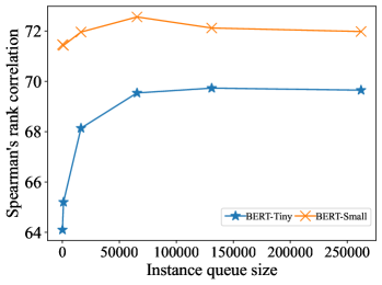
Figure 4: The comparison between various queue sizes, such as 128, 1024, 16384, 65536, 131072, and 262144. We average Spearman’s rank correlation across the seven STS benchmarks and test on small PLMs, i.e., BERT-Tiny and BERT-Small.

5.3.3 Data augmentation choice

This experiment evaluates the effect of different augmentation schemes widely used in sentence representation learning: (i) two back-translations (default), (ii) mask language model 15%, (iii) synonym replacement (one-word replacement), (iii) dropout mask, and (iv) using the same back-translation ($\mathcal{T}=\mathcal{T}^{\prime}$). We evaluate Spearman’s rank correlation on seven STS benchmark datasets. The experimental results are shown in Table 4 (Data augmentation studies).

As expected, changing back-translation to other augmentation schemes decreases the performance in all cases. For instance, the performance of BERT-Tiny drops from 69.73 to 64.07 when we change from two back-translations to only one back-translation. This is because the two back-translation schemes generate high-quality synonym text pairs (different syntax but same meaning), which help sentence representation to distinguish positive and negative samples in the embedding space. In contrast, other augmentation techniques produce either incorrect or similar pair texts, which are not useful for sentence representation learning.

Data augmentation analysis. To validate our data augmentation strategy, we assess the syntax and semantic scores on our augmented datasets. We utilized the edit distance metric to evaluate the syntax changes (dissimilarity) in the augmented datasets compared to the original dataset. Additionally, we employed cosine similarity to evaluate the semantic consistency between the original and augmented embeddings. Our base encoders in this analysis were BERT-Tiny-SCT and BERT-Tiny-DiffCSE.

The results, as presented in Table 5, revealed that although MLM produced the highest string dissimilarity, it failed to preserve semantic from the original texts, resulting in significant changes to syntax and semantic. In contrast, the synonym augment scheme exhibited higher embedding similarity than MLM, as it maintained the original texts to a greater extent, resulting in minimal changes to syntax and semantic. Interestingly, back-translation produced favorable results in both string and embedding similarity. While the syntax was altered, the semantic remained unchanged, indicating reasonable performance in maintaining the core semantic meaning. While the string dissimilarity of back-translation was slightly lower than that of MLM (with only one character difference on average), back-translation achieved higher similarities in the base encoders’ embeddings.

Method	String Dissim.	Embedding Sim.
		SCT	DiffCSE
Synonym	6.59 $\pm$ 4.30	0.94	0.97
MLM	13.37 $\pm$ 7.67	0.85	0.94
BT	12.32 $\pm$ 9.31	0.98	0.97

Table 5: We evaluate the string dissimilarity and embedding similarity on our training and augmentation datasets. For the string dissimilarity, we use edit distance to evaluate the changes in the augmentation dataset. For the embedding similarity, we use cosine similarity to evaluate the identical of the original and augmentation dataset.

These findings corroborate the results of our data augmentation choices, as shown in Table 4, where we emphasize that data augmentation methods with desirable properties exhibit high string dissimilarity and embedding similarity. The efficacy of back-translation, in particular, highlights its potential as a suitable data augmentation technique for preserving both syntax and semantic consistency, making it a promising technique for enhancing the performance of embedding space.

5.3.4 Summary of Design Analysis.

As shown in Table 4, we present the desired components in the SCT framework. We found that applying a technique from computer vision requires careful consideration of the architecture and data augmentation schemes. The experimental results from the model and loss studies demonstrate that using contrastive learning similar to SimCSE Gao et al. (2021) or using a momentum encoder similar to MoCo He et al. (2020); Chen et al. (2020) produce poorer performance than our setting (small PLMs). This is because of the fact that small PLMs necessitate more guidance, as discussed in Section 3. Thus, the similarity-score-distribution learning paradigm employed in our framework demonstrates promising results in enhancing the performance of small PLMs. However, it is worth noting that applying the similarity-score-distribution learning paradigm from Fang et al. (2021) without making any adjustments adversely affects the model’s performance more than any other setting, i.e., the performance of BERT-Tiny decreased by 7.82 points when we changed from cross-view (our work) to identical-view (computer vision).

Regarding the data augmentation studies (Section 5.3.3), we found that using two-back translations produced the most effective augmented sentences compared to MLM or synonym replacement. With these findings, we require to adjust architectures, loss, and data augmentation from previous works, which achieved SOTA performance in small PLMs. These insightful findings necessitate the adaptation of architectures, loss functions, and data augmentation approaches from prior works. By carefully considering these adjustments, we can further enhance the capabilities and efficiency of small PLMs in various NLP tasks.

5.4 Distillation Studies

In this subsection, we study the components of our distillation method as follows. In Section 5.4.1, we provide an ablation study on the model and loss function. Section 5.4.2 presents an analysis of the distillation loss.

5.4.1 Distillation Design

This study illustrates the efficacy of SCT within distillation settings. An ablation study has been meticulously conducted to elucidate that all constituent elements of SCT contribute to the overall performance. In particular, we demonstrate the ablation study of the self-supervised loss $\mathcal{L}_{\text{SCT}}$ in distillation settings using the setup from Table 4.

The findings in Table 6 highlight the importance of adhering to the default SCT configuration, as any departure from it incurs a notable performance decrement. The analysis distinctly reveals that the most substantial penalties arise from the alterations involving Distribution$\rightarrow$Contrastive and Cross-view$\rightarrow$Identical-view adjustments. These results emphasize all components of SCT contribute to performance improvement. Any deviation from the default SCT setting results in a performance penalty.

Method	BERT-Tiny	BERT-Small
SCT-distillation	76.43	78.16
Model & loss studies
Distribution $\rightarrow$ Contrastive	$\downarrow$6.03	$\downarrow$3.26
Cross-view $\rightarrow$ Identical-view	$\downarrow$3.97	$\downarrow$1.43
$f_{\text{ref}}$ $\rightarrow$ a momentum encoder	$\downarrow$3.62	$\downarrow$0.97
KL $\rightarrow$ CE	$\downarrow$3.43	$\downarrow$0.98
No MLPs	$\downarrow$4.14	$\downarrow$2.46

Table 6: Ablation studies on model & loss of our distillation method. We evaluate the performance of these studies on the average score across seven STS datasets.

5.4.2 Distillation Loss

This experiment demonstrates the efficacy of our novel approach involving self-supervised and distillation losses. We investigate the impact of using a distillation loss alone and the benefits of integrating both distillation and self-supervised losses. In particular, we explore the utility of our SCT loss as a bootstrapping mechanism for existing distillation methods. We also demonstrate a common distillation loss by minimizing the discrepancy between $z^{\text{large}}$ and $z^{\theta}$ with Mean Square Error ($\mathcal{L}_{\text{MSE}}$).

Table 7 presents the experimental results for two scenarios: (i) using only a distillation loss and (ii) incorporating both self-supervised and distillation losses. In addition, we highlight the improvement with the up arrow ($\uparrow$). Our experimental findings consistently demonstrate that including the SCT loss significantly enhances the performance of existing distillation methods across the board. For example, the SCT loss yields substantial performance boosts of 3.28 and 4.50 for $\mathcal{L}_{\text{CD}}$ and $\mathcal{L}_{\text{MSE}}$ methods on BERT-Tiny, respectively. Moreover, we improve the performance of ConGen and CKD methods to a level comparable with $\mathcal{L}_{\text{CD}}+\mathcal{L}_{\text{SCT}}$. We do this using SCT as the bootstrapping loss. These results underscore the advantages of combining distillation and self-supervised losses to achieve enhanced performance in small PLMs. Furthermore, our SCT loss demonstrates its efficacy as a reliable bootstrapping loss for distillation methods, highlighting its potential as a valuable tool for improving the performance of distillation-based approaches.

Method	BERT-Tiny		BERT-Small
$\mathcal{L}_{\text{CD}}$	71.93		74.41
$\mathcal{L}_{\text{CD}}+\mathcal{L}_{\text{SCT}}$	76.43	$\uparrow$4.50	78.16	$\uparrow$3.75
$\mathcal{L}_{\text{MSE}}$	71.42		73.16
$\mathcal{L}_{\text{MSE}}+\mathcal{L}_{\text{SCT}}$	74.70	$\uparrow$3.28	76.11	$\uparrow$2.95
$\mathcal{L}_{\text{ConGen}}$	75.89		77.31
$\mathcal{L}_{\text{ConGen}}+\mathcal{L}_{\text{SCT}}$	76.36	$\uparrow$0.47	77.87	$\uparrow$0.56
$\mathcal{L}_{\text{CKD}}$	75.34		76.47
$\mathcal{L}_{\text{CKD}}+\mathcal{L}_{\text{SCT}}$	76.06	$\uparrow$0.72	76.94	$\uparrow$0.46

Table 7: We evaluate the performance of these studies on the average score across seven STS datasets.

6 Conclusion

We propose a self-supervised sentence representation learning method called Self-Supervised Cross-View Training (SCT). The observation inspires our work that smaller models, when constructed in a self-supervised setting, tend to perform poorly or collapse altogether. We hypothesize that this problem can be addressed by providing additional learning guidance to facilitate the self-referencing mechanism in the self-supervised learning pipeline.

Our work consists of three key contributions. First, at the framework level, we formulate a cross-view comparison pipeline to improve the self-referencing mechanism by enabling cross-comparison between two input views. In addition, our framework allows using two input views formulated from the same or different PLMs. Second, to facilitate the learning process, we also design a new technique to measure the discrepancy between two cross-view outputs. Instead of comparing them directly, we use similarity score distributions. Third, we conducted extensive sets of experimental studies to compare our method against existing competitors and to analyze our design decisions.

The experimental results on the STS tasks show that our method dominates all competitors in the cases of PLMs with less than 100M parameters. With the help of the distillation loss, our method improves the performance of small PLMs better than that of large PLMs. Moreover, our method outperforms competitive methods for all PLMs on the downstream tasks. Furthermore, the results also confirm that the cross-view comparison pipeline and similarity score distribution comparison are crucial to performance improvement. These findings imply that smaller PLMs benefit from our judiciously designed guidance in a self-supervised setting.

References

- Agirre et al. (2015) Eneko Agirre, Carmen Banea, Claire Cardie, Daniel Cer, Mona Diab, Aitor Gonzalez-Agirre, Weiwei Guo, Iñigo Lopez-Gazpio, Montse Maritxalar, Rada Mihalcea, German Rigau, Larraitz Uria, and Janyce Wiebe. 2015. SemEval-2015 task 2: Semantic textual similarity, English, Spanish and pilot on interpretability. In SemEval 2015.
- Agirre et al. (2014) Eneko Agirre, Carmen Banea, Claire Cardie, Daniel Cer, Mona Diab, Aitor Gonzalez-Agirre, Weiwei Guo, Rada Mihalcea, German Rigau, and Janyce Wiebe. 2014. SemEval-2014 task 10: Multilingual semantic textual similarity. In SemEval 2014.
- Agirre et al. (2016) Eneko Agirre, Carmen Banea, Daniel Cer, Mona Diab, Aitor Gonzalez-Agirre, Rada Mihalcea, German Rigau, and Janyce Wiebe. 2016. SemEval-2016 task 1: Semantic textual similarity, monolingual and cross-lingual evaluation. In SemEval-2016.
- Agirre et al. (2012) Eneko Agirre, Daniel Cer, Mona Diab, and Aitor Gonzalez-Agirre. 2012. SemEval-2012 task 6: A pilot on semantic textual similarity. In *SEM 2012: The First Joint Conference on Lexical and Computational Semantics – Volume 1: Proceedings of the main conference and the shared task, and Volume 2: Proceedings of the Sixth International Workshop on Semantic Evaluation (SemEval 2012).
- Agirre et al. (2013) Eneko Agirre, Daniel Cer, Mona Diab, Aitor Gonzalez-Agirre, and Weiwei Guo. 2013. *SEM 2013 shared task: Semantic textual similarity. In Second Joint Conference on Lexical and Computational Semantics (*SEM), Volume 1: Proceedings of the Main Conference and the Shared Task: Semantic Textual Similarity.
- Bowman et al. (2015) Samuel R. Bowman, Gabor Angeli, Christopher Potts, and Christopher D. Manning. 2015. A large annotated corpus for learning natural language inference. In EMNLP 2015.
- Brutzkus and Globerson (2019) Alon Brutzkus and Amir Globerson. 2019. Why do larger models generalize better? A theoretical perspective via the XOR problem. In Proceedings of the 36th International Conference on Machine Learning, volume 97 of Proceedings of Machine Learning Research, pages 822–830. PMLR.
- Cao et al. (2022) Rui Cao, Yihao Wang, Yuxin Liang, Ling Gao, Jie Zheng, Jie Ren, and Zheng Wang. 2022. Exploring the impact of negative samples of contrastive learning: A case study of sentence embedding. In Findings of the Association for Computational Linguistics: ACL 2022, pages 3138–3152, Dublin, Ireland. Association for Computational Linguistics.
- Cer et al. (2017) Daniel Cer, Mona Diab, Eneko Agirre, Iñigo Lopez-Gazpio, and Lucia Specia. 2017. SemEval-2017 task 1: Semantic textual similarity multilingual and crosslingual focused evaluation. In Proceedings of the 11th International Workshop on Semantic Evaluation (SemEval-2017).
- Chen et al. (2020) Xinlei Chen, Haoqi Fan, Ross Girshick, and Kaiming He. 2020. Improved baselines with momentum contrastive learning.
- Chen and He (2021) Xinlei Chen and Kaiming He. 2021. Exploring simple siamese representation learning. In Proceedings of the IEEE/CVF Conference on Computer Vision and Pattern Recognition (CVPR), pages 15750–15758.
- Chuang et al. (2022) Yung-Sung Chuang, Rumen Dangovski, Hongyin Luo, Yang Zhang, Shiyu Chang, Marin Soljacic, Shang-Wen Li, Scott Yih, Yoon Kim, and James Glass. 2022. DiffCSE: Difference-based contrastive learning for sentence embeddings. In Proceedings of the 2022 Conference of the North American Chapter of the Association for Computational Linguistics: Human Language Technologies, pages 4207–4218, Seattle, United States. Association for Computational Linguistics.
- Cohan et al. (2020) Arman Cohan, Sergey Feldman, Iz Beltagy, Doug Downey, and Daniel S. Weld. 2020. Specter: Document-level representation learning using citation-informed transformers. In ACL.
- Conneau and Kiela (2018) Alexis Conneau and Douwe Kiela. 2018. Senteval: An evaluation toolkit for universal sentence representations. In Proceedings of the Eleventh International Conference on Language Resources and Evaluation, LREC 2018, Miyazaki, Japan, May 7-12, 2018. European Language Resources Association (ELRA).
- Devlin et al. (2019) Jacob Devlin, Ming-Wei Chang, Kenton Lee, and Kristina Toutanova. 2019. BERT: pre-training of deep bidirectional transformers for language understanding. In NAACL-HLT 2019.
- Fang et al. (2020) Hongchao Fang, Sicheng Wang, Meng Zhou, Jiayuan Ding, and Pengtao Xie. 2020. Cert: Contrastive self-supervised learning for language understanding.
- Fang et al. (2021) Zhiyuan Fang, Jianfeng Wang, Lijuan Wang, Lei Zhang, Yezhou Yang, and Zicheng Liu. 2021. SEED: self-supervised distillation for visual representation. In ICLR 2021.
- Gao et al. (2021) Tianyu Gao, Xingcheng Yao, and Danqi Chen. 2021. SimCSE: Simple contrastive learning of sentence embeddings. In Proceedings of the 2021 Conference on Empirical Methods in Natural Language Processing, pages 6894–6910, Online and Punta Cana, Dominican Republic. Association for Computational Linguistics.
- Grill et al. (2020) Jean-Bastien Grill, Florian Strub, Florent Altché, Corentin Tallec, Pierre Richemond, Elena Buchatskaya, Carl Doersch, Bernardo Avila Pires, Zhaohan Guo, Mohammad Gheshlaghi Azar, Bilal Piot, koray kavukcuoglu, Remi Munos, and Michal Valko. 2020. Bootstrap your own latent - a new approach to self-supervised learning. In Advances in Neural Information Processing Systems, volume 33, pages 21271–21284. Curran Associates, Inc.
- He et al. (2020) Kaiming He, Haoqi Fan, Yuxin Wu, Saining Xie, and Ross Girshick. 2020. Momentum contrast for unsupervised visual representation learning. In 2020 IEEE/CVF Conference on Computer Vision and Pattern Recognition (CVPR), pages 9726–9735.
- Kim et al. (2021) Taeuk Kim, Kang Min Yoo, and Sang-goo Lee. 2021. Self-guided contrastive learning for BERT sentence representations. In ACL/IJCNLP 2021.
- Klein and Nabi (2022) Tassilo Klein and Moin Nabi. 2022. SCD: Self-contrastive decorrelation of sentence embeddings. In Proceedings of the 60th Annual Meeting of the Association for Computational Linguistics (Volume 2: Short Papers), pages 394–400, Dublin, Ireland. Association for Computational Linguistics.
- Lei et al. (2016) Tao Lei, Hrishikesh Joshi, Regina Barzilay, Tommi Jaakkola, Kateryna Tymoshenko, Alessandro Moschitti, and Lluís Màrquez. 2016. Semi-supervised question retrieval with gated convolutions. In Proceedings of the 2016 Conference of the North American Chapter of the Association for Computational Linguistics: Human Language Technologies, pages 1279–1289, San Diego, California. Association for Computational Linguistics.
- Li et al. (2020) Bohan Li, Hao Zhou, Junxian He, Mingxuan Wang, Yiming Yang, and Lei Li. 2020. On the sentence embeddings from pre-trained language models. In EMNLP 2020.
- Limkonchotiwat et al. (2022) Peerat Limkonchotiwat, Wuttikorn Ponwitayarat, Lalita Lowphansirikul, Can Udomcharoenchaikit, Ekapol Chuangsuwanich, and Sarana Nutanong. 2022. ConGen: Unsupervised control and generalization distillation for sentence representation. In Findings of the Association for Computational Linguistics: EMNLP 2022, pages 6467–6480, Abu Dhabi, United Arab Emirates. Association for Computational Linguistics.
- Liu et al. (2021) Fangyu Liu, Ivan Vulić, Anna Korhonen, and Nigel Collier. 2021. Fast, effective, and self-supervised: Transforming masked language models into universal lexical and sentence encoders. In Proceedings of the 2021 Conference on Empirical Methods in Natural Language Processing, pages 1442–1459, Online and Punta Cana, Dominican Republic. Association for Computational Linguistics.
- Liu et al. (2019) Yinhan Liu, Myle Ott, Naman Goyal, Jingfei Du, Mandar Joshi, Danqi Chen, Omer Levy, Mike Lewis, Luke Zettlemoyer, and Veselin Stoyanov. 2019. Roberta: A robustly optimized bert pretraining approach.
- Loshchilov and Hutter (2019) Ilya Loshchilov and Frank Hutter. 2019. Decoupled weight decay regularization. In 7th International Conference on Learning Representations, ICLR 2019, New Orleans, LA, USA, May 6-9, 2019. OpenReview.net.
- Marelli et al. (2014) Marco Marelli, Stefano Menini, Marco Baroni, Luisa Bentivogli, Raffaella Bernardi, and Roberto Zamparelli. 2014. A SICK cure for the evaluation of compositional distributional semantic models. In Proceedings of the Ninth International Conference on Language Resources and Evaluation (LREC’14), pages 216–223, Reykjavik, Iceland. European Language Resources Association (ELRA).
- Reimers and Gurevych (2019) Nils Reimers and Iryna Gurevych. 2019. Sentence-BERT: Sentence embeddings using Siamese BERT-networks. In Proceedings of the 2019 Conference on Empirical Methods in Natural Language Processing and the 9th International Joint Conference on Natural Language Processing (EMNLP-IJCNLP), pages 3982–3992, Hong Kong, China. Association for Computational Linguistics.
- Sanh et al. (2019) Victor Sanh, Lysandre Debut, Julien Chaumond, and Thomas Wolf. 2019. Distilbert, a distilled version of bert: smaller, faster, cheaper and lighter.
- Tao et al. (2022) Chenxin Tao, Honghui Wang, Xizhou Zhu, Jiahua Dong, Shiji Song, Gao Huang, and Jifeng Dai. 2022. Exploring the equivalence of siamese self-supervised learning via A unified gradient framework. In IEEE/CVF Conference on Computer Vision and Pattern Recognition, CVPR 2022, New Orleans, LA, USA, June 18-24, 2022, pages 14411–14420. IEEE.
- Tejankar et al. (2021) Ajinkya Tejankar, Soroush Abbasi Koohpayegani, Vipin Pillai, Paolo Favaro, and Hamed Pirsiavash. 2021. Isd: Self-supervised learning by iterative similarity distillation. In 2021 IEEE/CVF International Conference on Computer Vision (ICCV), pages 9589–9598.
- Turc et al. (2019) Iulia Turc, Ming-Wei Chang, Kenton Lee, and Kristina Toutanova. 2019. Well-read students learn better: On the importance of pre-training compact models. arXiv preprint arXiv:1908.08962v2.
- Wang et al. (2021) Kexin Wang, Nils Reimers, and Iryna Gurevych. 2021. TSDAE: Using transformer-based sequential denoising auto-encoderfor unsupervised sentence embedding learning. In Findings of the Association for Computational Linguistics: EMNLP 2021, pages 671–688, Punta Cana, Dominican Republic. Association for Computational Linguistics.
- Wang et al. (2020) Wenhui Wang, Furu Wei, Li Dong, Hangbo Bao, Nan Yang, and Ming Zhou. 2020. Minilm: Deep self-attention distillation for task-agnostic compression of pre-trained transformers. In NeurIPS 2020.
- Williams et al. (2018) Adina Williams, Nikita Nangia, and Samuel Bowman. 2018. A broad-coverage challenge corpus for sentence understanding through inference. In NAACL 2018.
- Wu et al. (2021) Xing Wu, Chaochen Gao, Jue Wang, Liangjun Zang, Zhongyuan Wang, and Songlin Hu. 2021. Disco: Effective knowledge distillation for contrastive learning of sentence embeddings.
- Yan et al. (2021) Yuanmeng Yan, Rumei Li, Sirui Wang, Fuzheng Zhang, Wei Wu, and Weiran Xu. 2021. ConSERT: A contrastive framework for self-supervised sentence representation transfer. In Proceedings of the 59th Annual Meeting of the Association for Computational Linguistics and the 11th International Joint Conference on Natural Language Processing (Volume 1: Long Papers), pages 5065–5075, Online. Association for Computational Linguistics.
- Zbontar et al. (2021) Jure Zbontar, Li Jing, Ishan Misra, Yann LeCun, and Stephane Deny. 2021. Barlow twins: Self-supervised learning via redundancy reduction. In Proceedings of the 38th International Conference on Machine Learning, volume 139 of Proceedings of Machine Learning Research, pages 12310–12320. PMLR.
- Zhang et al. (2022a) Chaoning Zhang, Kang Zhang, Chenshuang Zhang, Trung X. Pham, Chang D. Yoo, and In So Kweon. 2022a. How does simsiam avoid collapse without negative samples? A unified understanding with self-supervised contrastive learning. In The Tenth International Conference on Learning Representations, ICLR 2022, Virtual Event, April 25-29, 2022. OpenReview.net.
- Zhang et al. (2022b) Dejiao Zhang, Wei Xiao, Henghui Zhu, Xiaofei Ma, and Andrew Arnold. 2022b. Virtual augmentation supported contrastive learning of sentence representations. In Findings of the Association for Computational Linguistics: ACL 2022, pages 864–876, Dublin, Ireland. Association for Computational Linguistics.
- Zhang et al. (2021) Yan Zhang, Ruidan He, Zuozhu Liu, Lidong Bing, and Haizhou Li. 2021. Bootstrapped unsupervised sentence representation learning. In Proceedings of the 59th Annual Meeting of the Association for Computational Linguistics and the 11th International Joint Conference on Natural Language Processing (Volume 1: Long Papers), pages 5168–5180, Online. Association for Computational Linguistics.
- Zhang et al. (2020) Yan Zhang, Ruidan He, Zuozhu Liu, Kwan Hui Lim, and Lidong Bing. 2020. An unsupervised sentence embedding method by mutual information maximization. In EMNLP 2020.
- Zheng et al. (2021) Mingkai Zheng, Shan You, Fei Wang, Chen Qian, Changshui Zhang, Xiaogang Wang, and Chang Xu. 2021. Ressl: Relational self-supervised learning with weak augmentation. In Advances in Neural Information Processing Systems 34: Annual Conference on Neural Information Processing Systems 2021, NeurIPS 2021, December 6-14, 2021, virtual, pages 2543–2555.
- Zhou et al. (2022) Kun Zhou, Beichen Zhang, Xin Zhao, and Ji-Rong Wen. 2022. Debiased contrastive learning of unsupervised sentence representations. In Proceedings of the 60th Annual Meeting of the Association for Computational Linguistics (Volume 1: Long Papers), pages 6120–6130, Dublin, Ireland. Association for Computational Linguistics.