Spatial Process Approximations: Assessing Their Necessity

Abstract

In spatial statistics and machine learning, the kernel matrix plays a pivotal role in prediction, classification, and maximum likelihood estimation. A thorough examination reveals that for large sample sizes, the kernel matrix becomes ill-conditioned, provided the sampling locations are fairly evenly distributed. This condition poses significant challenges to numerical algorithms used in prediction and estimation computations and necessitates an approximation to prediction and the Gaussian likelihood. A review of current methodologies for managing large spatial data indicates that some fail to address this ill-conditioning problem. Such ill-conditioning often results in low-rank approximations of the stochastic processes. This paper introduces various optimality criteria and provides solutions for each.

1 Introduction

Spatial data collected from sampling sites across a continuous region are considered to be a partial realization of an underlying stochastic process. The ultimate objective for such data is often spatial interpolation. Linear interpolation is commonly used due to its simplicity, and Kriging is a technique for achieving the best linear unbiased interpolation which only relies on the first two moments of the stochastic process. It depends on solving linear equations that involve an $n\times n$ covariance matrix $V$, where $n$ is the number of sampling sites. The covariance matrix also appears in the Gaussian likelihood function used in both maximum likelihood estimation and Bayesian analysis of spatial data. In Kriging and statistical inferences, the inverse of the covariance matrix (also known as the precision matrix) is employed. However, advances in technology have led to sample sizes that can be thousands or even millions, making matrix inversion computationally challenging and unstable. As a result, various methods have been proposed to use approximate models to circumvent this problem.

Several methods leverage the computational efficiency of sparse matrices. One such technique is covariance tapering, which approximates $V$ using a sparse matrix (Furrer et al., 2006; Kaufman et al., 2008; Stein et al., 2013). Studies have demonstrated that an appropriate taper leads to asymptotically optimal interpolation and efficient estimation (Furrer et al., 2006; Du et al., 2009). Another approach involves using block diagonal matrices for covariance matrices (Stein et al., 2004; Eidsvik et al., 2014). Some methods alternatively employ a sparse precision matrix by assuming conditional independence (Rue et al., 2009; Lindgren et al., 2011; Datta et al., 2016a, b; Stroud et al., 2017; Guinness, 2018). Other techniques utilize low-rank approximations to Gaussian processes, such as discrete process convolutions (Higdon, 2002; Lemos and Sansó, 2009), fixed rank kriging (Cressie and Johannesson, 2008; Kang and Cressie, 2011; Katzfuss and Cressie, 2011), predictive processes (Banerjee et al., 2008; Finley et al., 2009), lattice kriging (Nychka et al., 2015). For a review of these methods, refer to Sun et al. (2012), and for comparisons, see Bradley et al. (2016) and Heaton et al. (2019).

These methods were primarily designed to enhance computational efficiency and stability, especially given the challenges and computational demands of exact kriging and maximum likelihood estimation. However, our study adopts a more theoretical perspective. We provide a rigorous proof that under general conditions, both the matrix $V$ and its inverse are ill-conditioned. This characteristic makes the computation of kriging coefficients using numerically stable algorithms nearly impossible. Merely boosting computational power is not a panacea for this problem. Therefore, approximations of either $V$ or $V^{-1}$ become necessary. This leads to the need for approximations of the covariance matrix or the precision matrix, as well as the search for approximate methods for Kriging and Gaussian likelihood estimation.

Our results are based on the investigation of the decay of eigenvalues of covariance matrices, which has been an understudied topic. In the case of stationary covariance, previous research has provided upper bounds and established decay rates for the eigenvalue under certain conditions. For example, Schaback (1995) provided an upper bound for the smallest eigenvalue when the sampling sites are nearly uniformly spaced in a bounded region, while Belkin et al. (2019) established a decay rate in the case of Gaussian stationary covariance functions. Tang et al. (2021) generalized the results to the Matérn family. When the sampling locations are assumed to be an independent sample from some probability distribution, a central limit theorem has been established for the eigenvalues of the normalized kernel matrix (Koltchinskii and Giné, 2000) and probabilistic error bounds have been established for finite samples (Braun, 2006; Jia and Liao, 2009). However, we provide an error bound for the tail sum of the eigenvalues without requiring stationarity or independence of sampling locations. Our results have potential applications beyond spatial statistics as the covariance matrix, also known as the kernel matrix in machine learning, is used in a range of fields including machine learning (Schölkopf and Smola, 2002), computer vision (Bagnell et al., 2009), computer experiment (O’Hagan, 1978; Currin et al., 1991), pattern recognition (Shawe-Taylor and Cristianini, 2004), signal processing (Raykar and Duraiswami, 2007), computational biology (Schölkopf et al., 2004), robotics (Deisenroth et al., 2015), and pre-trained Gaussian process (Wang et al., 2023).

The remainder of this paper is structured as follows. In Section 2, we present the principal theorem pertaining to the eigenvalues of the kernel matrix. This main result prompts us to examine low-rank models. Consequently, in Section 3, we explore a specific construction of low-rank approximation and employ the pseudo-inverse for Kriging. In Section 4, we introduce several criteria for optimal low-rank approximation and discuss their respective solutions. The proofs for the theorems are provided in the Appendix.

2 Eigenvalues of Kernel Matrix

Throughout this paper, we use $H$ to denote the Hilbert space generated by $Y(s),s\in D\subset R^{d}$ with the inner product $(Y(s),Y(x))_{H}=K(s,x)$. For any $Y\in H$ and a subspace $W\subset H$, $\Pi[Y|W]$ represents the projection of $Y$ onto $W$. For $x\in R^{d}$, $\|x\|$ signifies the Euclidean norm. Additionally, for a subset $D\subset R^{d}$, $|D|$ denotes the area or volume of $D$, and $\Delta(D)=\sup\{\|x-y\|,x,y\in D\}$ refers to the supremum of distance between any pair of points in $D$.

Before presenting the main result, we will briefly discuss the Karhunen-Loève (KL) expansion and its properties, which will provide insight into the main result and facilitate subsequent proofs. For a more comprehensive treatment of the KL expansion, we direct readers to Ghanem and Spanos (1991). Consider a second-order process $Y(s)$ with mean 0, where $s\in D$ and $D$ is a compact subset in $R^{d}$. Let its covariance function $K(s,x)$ be continuous in $(s,x)$. Then, $Y(s)$ can be represented as:

$$Y(s)=\sum_{i=1}^{\infty}\sqrt{\lambda_{i}}\varphi_{i}(s)\xi_{i}$$ (1)

where $\lambda_{i}\geq 0$ decreases to 0 as $i\to\infty$, $\xi_{i}$ are uncorrelated random variables with unit variances, and the functions $\varphi_{i}(s)$ constitute an orthonormal system, that is,

$$\int_{D}\varphi_{i}(s)\varphi_{j}(s)ds=\delta_{ij}.$$

The convergence in (1) is in the $L_{2}$ sense. It follows that

$$K(s,x)=\sum_{i=1}^{\infty}\lambda_{i}\varphi_{i}(s)\varphi_{i}(x).$$ (2)

which is called the Mercer’s Theorem. A subsequent property is that the eigenvalues are a convergent series, i.e.,

$$\sum_{i=1}^{\infty}\lambda_{i}=\int_{D}K(s,s)ds<\infty.$$ (3)

Therefore $\sum_{i>k}\lambda_{i}\to 0$ if $k\to\infty$. We might approximate the process $Y(s)$ by truncating the KL expansion and the integrated mean squared error becomes

$$\int_{D}E\left(Y(s)-\sum_{i=1}^{k}\sqrt{\lambda_{i}}\varphi_{i}(s)\xi_{i}\right)^{2}ds=\sum_{i>k}\lambda_{i}.$$

Indeed, the truncated KL expansion is optimal in the following sense,

$$\min\int_{D}E\left(Y(s)-\sum_{i=1}^{k}a_{i}(s)Z_{i}\right)^{2}ds=\sum_{i>k}\lambda_{i}$$ (4)

where the minimum is over all square integrable functions $a_{i}(s)$ and random variables $Z_{i}$.

The explicit convergence rates of the eigenvalues $\lambda_{i}$ have been studied in mathematical literature. For example, König (1986) and Pietsch (1987) studied convergence of eigenvalues of bounded operators on compact sets. Schaback and Wendland (2002) and Santin and Schaback (2016) established explicit rates for $\lambda_{i}$ of radial basis kernels when the spectral density satisfies some tail properties.

Now consider that the process is observed at $n$ locations, $s_{i},~{}i=1,2,\ldots,n$ and write $V_{n}=(K(s_{i},s_{j}))_{i,j=1}^{n}$. Let $\lambda_{n,i}$ be the $i$th largest eigenvalue of $V_{n}$ and $\mbox{\boldmath$u$}_{i}$ the corresponding eigenvector. The eigenvalues depend on $n$ obviously, and we will suppress $n$ when it does not lead to confusion. Then $\mbox{\boldmath$Y$}=(Y(s_{1}),Y(s_{2}),\ldots,Y(s_{n}))^{\prime}$ as a random vector in $R^{n}$ can be written in the form of orthogonal projection

$$\mbox{\boldmath$Y$}=\sum_{i=1}^{n}(\mbox{\boldmath$Y$}^{\prime}\mbox{\boldmath$u$}_{i})\mbox{\boldmath$u$}_{i}.$$ (5)

It is easy to see that the terms $Z_{i}=\mbox{\boldmath$Y$}^{\prime}\mbox{\boldmath$u$}_{i}$ are uncorrelated and $\text{Var}(Z_{i})=\lambda_{n,i}$. The $Z_{i}$’s are referred to as the principal components of $Y$. We can write

$$Y(s_{j})=\sum_{i=1}^{n}\sqrt{\lambda_{n,i}}u_{ij}\xi_{i}$$ (6)

where $\xi_{i}=Z_{i}/\sqrt{\lambda_{n,i}}$ is standardized to have a variance of 1, and $u_{ij}$ is the $i$th element of $\mbox{\boldmath$u$}_{j}$. We see that (6) is similar to (1). Indeed, it is referred to as the discrete KL expansion (e.g., Dür, 1998). There is a similar property to (4) which we will introduce in the next section. The KL expansion and the discrete KL expansion are both special cases of the spectral theory for compact transformation in Hilbert spaces.

Understanding the behavior of the eigenvalues $\lambda_{n,i}$ is both practically important and intriguing. A handful of available results indicate that the ratio $\lambda_{n,i}/n$ approaches $\lambda_{i}$ as $n$ becomes large. For instance, probabilistic error bounds for the difference $\lambda_{n,i}/n-\lambda_{i}$ were provided by Braun (2006) and Jia and Liao (2009). Further, Belkin (2018) and Tang et al. (2021) established upper bounds for $\lambda_{n,i}/n$ in cases where the covariance function belongs to the Gaussian and the Matern families, respectively. These bounds are analogous to those for $\lambda_{i}$.

We now state a key result on the decay of $\lambda_{n,i}$. We show under some regularity conditions on the sampling locations $s_{i}$,

$$\sum_{i=k+1}^{n}\lambda_{n,i}/n\leq c_{0}\sum_{i=k+1}^{n}\lambda_{i}+o(1)\quad\mbox{ as }k,n\to\infty,$$ (7)

where $c_{0}$ is a constant that depends on $K$ but not $n$. This leads to the following main result.

Theorem 1

Let $s_{i},i=1,2,\ldots,n$ be distinct points in a compact subset $D\in R^{d}$ such that the Voronoi diagram defined by

$$D_{n,i}=\{x\in D:\|x-s_{i}\|=\min_{j}\|x-s_{j}\|\}$$

satisfies

$$\max_{1\leq i\leq n}\Delta(D_{n,i})\to 0,\mbox{ and }\sup_{n}\frac{\max_{1\leq i\leq n}|D_{n,i}|}{\min_{1\leq i\leq n}|D_{n,i}|}<\gamma$$ (8)

for some constant $\gamma$. If $K(s,x)$ is continuous in $(s,x)$, then

$$(1/n)\sum_{i=k+1}^{n}\lambda_{n,i}\leq C_{1}\sum_{i=k+1}^{n}\lambda_{i}+C_{2}(1/c(\delta_{\max})-1)$$ (9)

where $C_{i}$ are constants that do not depend on $n$ but may depend on $K$, $\delta_{\max}=\max_{i}\Delta(D_{n,i})$, and the function $c(\delta)$ is defined as

$$c(\delta)=\inf\{(K(x_{1},x_{2})/K(x_{2},x_{2}))^{2}:\|x_{1}-x_{2}\|\leq\delta,x_{1},x_{2}\in D\}.$$ (10)

Conditions in (8) indicate that the locations become increasingly dense in $D$ and are not too unevenly scattered. The second term in the right-hand side of (9) depends on the behavior of the kernel near the origin. The term necessarily reflects the effect of configuration of the locations $s_{i}$. For example, if some of $s_{i}$ are extremely close to each other, some rows of $V_{n}$ will be nearly identical to each other. Consequently, $V_{n}$ will be nearly singular or its smallest eigenvalues are close to 0. How close they are to 0 depends on the local behavior of the kernel function.

We can show that $\lambda_{n,1}/n$ is bounded below from 0. The next corollary immediately follows the theorem and implies that the kernel matrix $V_{n}$ is ill-conditioned as $n$ becomes large.

Corollary 1

Under the conditions of Theorem 1, for any $i\leq n$ such that $i\to\infty$, we have

$$\lambda_{n,1}/\lambda_{n,i}\to\infty.$$ (11)

Finally, we highlight that the theorem also indicates that the precision matrix is ill-conditioned because it shares the same condition number with the kernel matrix. There have been a burgeoning literature on sparse approximations to the precision matrix (e.g., Datta et al., 2016a; Guinness, 2018; Datta, 2021, 2022). It is probable that these approximations result in a matrix that is still ill-conditioned, particularly if the approximation is highly precise. However, the focus of this work is on the approximation of the covariance matrix rather than the precision matrix.

3 Pseudo-inverse for Spatial Prediction

3.1 Approximation of Kriging

Given $n$ observations at locations $s_{i}$, $i=1,2,\ldots,n$, the best linear unbiased prediction for $Y(s)$, assuming all variables have mean 0, is given by

$$\hat{Y}(s)=\mbox{\boldmath$\alpha$}(s)^{\prime}\mbox{\boldmath$Y$}$$ (12)

where $\mbox{\boldmath$\alpha$}(s)$ is the solution to $V_{n}\mbox{\boldmath$\alpha$}(s)=\mbox{\boldmath$k$}(s)$ for $\mbox{\boldmath$k$}(s)=(K(s,s_{i}),i=1,2,\ldots,n)^{\prime}$. Due to the ill-conditioning of the matrix $V_{n}$, solving the linear equations can become highly sensitive to small changes in the values in $\mbox{\boldmath$k$}(s)$, or a numerical solver for linear equations may fail to execute due to the extremely large condition number of $V_{n}$. In practice, this could mean that different methods such as the Gaussian elimination method, Cholesky decomposition, or QR decomposition might produce quite different results when obtaining the inverse matrix or solving linear equations. We mitigate this problem by projecting $Y(s)$ onto the $k$-dimensional subspace generated by the first $k$ principal components, and compare it with the kriging predictor in equation (12).

Let $Z_{i}$ be the principal components of $Y$, as in the previous section, and define

$$\tilde{Y}(s)=\Pi[Y(s)|Z_{1},Z_{2},\ldots,Z_{k}].$$ (13)

Since $Z_{i}$’s are uncorrelated and the variance $Var(Z_{i})=\lambda_{n,i}$ decreases rapidly, the main theorem implies that $Z_{1},Z_{2},\ldots,Z_{k}$ account most of the variation of $Y(s_{i})$’s for a sufficiently large $k$. Therefore, we might expect that $\tilde{Y}(s)$ to be quite close to the Kriging predictor $\hat{Y}(s)$ for some $k$ much less than $n$. The following theorem quantifies the predictive performance of the two predictors.

Theorem 2

$\tilde{Y}(s)$ can be expressed in terms of the $k$ eigenterms of $V_{n}$ as follows,

$$\tilde{Y}(s)=\mbox{\boldmath$k$}(s)^{\prime}\left(\sum_{i=1}^{k}\lambda_{n,i}^{-1}\mbox{\boldmath$u$}_{i}\mbox{\boldmath$u$}_{i}^{\prime}\right)\mbox{\boldmath$Y$}.$$

Furthermore, for any $s\in D$,

$$0<E|Y(s)-\tilde{Y}(s)|^{2}-E|Y(s)-\hat{Y}(s)|^{2}\leq\|\mbox{\boldmath$\alpha$}(s)\|_{2}^{2}\;\lambda_{n,k+1}$$

where $\mbox{\boldmath$\alpha$}(s)$ is the Kriging coefficients in (12) and $\|\mbox{\boldmath$\alpha$}(s)\|_{2}$ is the $L_{2}$ norm in the Euclidean space.

There are no theoretical results about the norm of $\mbox{\boldmath$\alpha$}(s)$ in general, but our empirical studies reveal the norm is often less than or equal to 1 though this may not be always true. When the norm if bounded, the difference between the two prediction variances decays at least as fast as $\lambda_{n,k+1}$. In the case of the Matérn kernel, Tang et al. (2021) has established the following upper bound:

$$\lambda_{n,k}\leq Cnk^{-2v/d-1}\mbox{ for all }k=1,\ldots,n$$

for some constant $C$. This bound can be used in the Metérn case to determine the appropriate $k$.

We note some properties of this approximate kriging prediction. Firstly,

$$\sum_{i=1}^{n}E\left(Y(s_{i})-\tilde{Y}(s_{i})\right)^{2}\leq\sum_{i=1}^{n}E\left(Y(s_{i})-\Pi[Y(s_{i})|S_{k}]\right)^{2}$$

for any $k$-dimensional subspace $S_{k}$ in $H_{n}$, the linear space spanned by $Y(s_{i}),i=1,2,\ldots,n$. We will prove this in the next section. As a result, the kriging prediction approximation demonstrates some optimal characteristic.

Secondly, the matrix $\sum_{i=1}^{k}\lambda_{n,i}^{-1}\mbox{\boldmath$u$}_{i}\mbox{\boldmath$u$}_{i}^{\prime}$ is the pseudo-inverse of the singular matrix $V_{n,k}=\sum_{i=1}^{k}\lambda_{n,i}\mbox{\boldmath$u$}_{i}\mbox{\boldmath$u$}_{i}^{\prime}$. For this reason, we will refer $\tilde{Y}(s)$ as the pseudo-kriging. It can be viewed as substituting the kernel matrix $V_{n}$ with its rank-$k$ approximation, $V_{n,k}$. The Eckart-Young Theorem (Golub and Loan, 2012) posits that $V_{n,k}$ minimizes $\|V-M\|$ for all $n\times n$ matrices $M$ of rank $k$, with the norm being either the Frobenius or $L_{2}$ norm. This optimal norm approximation is prevalent in machine learning.

However, to address the singularity of $V_{n,k}$, a perturbation term is typically introduced in the existing literature. As a result, the matrix $V_{n,k}+\tau I_{n}$ is used in its place, where $\tau$ is a sufficiently small positive number. As will be detailed later, the constant $\tau$ should be less than $\lambda_{n,k+1}$ to ensure optimal predictive performance. Nonetheless, selecting an excessively small value for $\tau$ might not improve the numerical stability of the matrix $V_{n,k}+\tau I_{n}$. Consequently, one may just use the pseudo-kriging as an alternative.

3.2 Numerical Studies on Eigenvalues Decay

Theorem 2 implies that the faster $\lambda_{n,k}$ decreases in $k$, the fewer terms will be needed to achieve the desirable approximation. In general, we may expect that $\lambda_{n,i}$ to be close to $\lambda_{i}$ when $n$ is large and the error bounds for the difference have been established. However, for a finite $n$, $\lambda_{n,i}$ also depends on the locations $s_{i}$.

In this section, we run some numerical studies to examine how fast the eigenvalues $\lambda_{n,k}$ decreases as $k$ increases for a large $n$. Specifically, we examine how fast $\sum_{i=1}^{k}\lambda_{n,i}$ decays as $k$ increases. We first consider three covariance functions from the Matérn family:

$$K_{1}(\mbox{\boldmath$h$})=\exp\left(-\frac{\|\mbox{\boldmath$h$}\|}{\phi}\right)\text{ for }\phi=0.25,$$

$$K_{2}(\mbox{\boldmath$h$})=\left(1+\frac{\sqrt{5}\|\mbox{\boldmath$h$}\|}{\phi}+\frac{5\|\mbox{\boldmath$h$}\|^{2}}{3\phi^{2}}\right)\exp\left(-\frac{\sqrt{5}\|\mbox{\boldmath$h$}\|}{\phi}\right)\text{ for }\phi=0.25,$$

$$K_{3}(\mbox{\boldmath$h$})=\exp\left(\frac{\|\mbox{\boldmath$h$}\|^{2}}{\phi}\right)\text{ for }\phi=0.1.$$

We plot the three covariance functions in Figure 1. The smoothness parameter of $K_{2}$ is $\nu=2.5$, and the corresponding process is twice differentiable. On the other hand, $K_{3}$ is infinitely differentiable. It’s well-known that the decay rate of the eigenvalues in the KL expansion is dependent on the smoothness parameter (Santin and Schaback, 2016). As the smoothness parameter increases, the eigenvalues decay faster. According to Theorem 1, we anticipate that larger smoothness parameters will result in more rapid decay of the eigenvalues $\lambda_{n,k}$.

For each of the three kernels, we compute the covariance matrix by assuming the sampling locations are at a 70 by 70 grid in the unit square: $\{(i/70.5,j/70.5),i,j=1,2,\ldots,70\}$. This results in a covariance matrix with dimensions of 4900 by 4900. We plot in Figure 2 the cumulative sum of $\sum_{i=1}^{k}\lambda_{n,i}$ against $k$. If $\lambda_{n,k}$ decreases faster, the cumulative sum approaches the asymptote faster. We see that for the differentiable cases, $k\leq 100$ provides sufficiently close approximation. Indeed, for $K_{3}$, the first 80 eigenvalues add to to 4899.995 and for $K_{2}$, the first 100 eigenvalues add up to 4893.675. For $K1$, the required number of eigenterms is much larger to achieve equally good approximation. When $k=500$, the sum of eigenvalues is 4657.037 or 95% of the total variation.

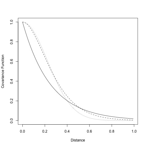
Figure 1: Plot of Three Covariance Functions ($K_{1}$=solid line, $K_{2}$=dashed line, $K_{3}$=dotted line).

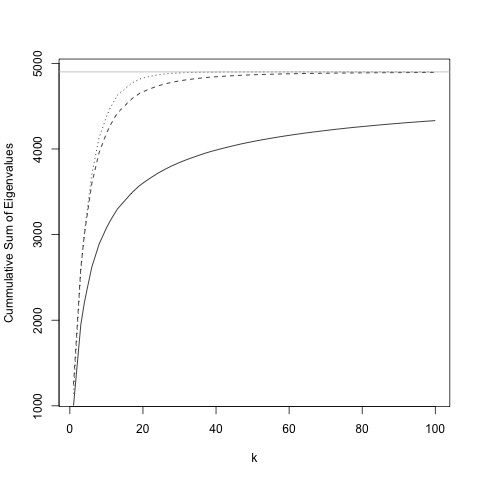
Figure 2: Cumulative Sums of Eigenvalues ($K_{1}$=solid line, $K_{2}$=dashed line, $K_{3}$=dotted line)

Lastly, we consider the polynomial covariance function that is used in some machine learning literature but not in spatial statistics, defined as

$$K_{4}(s,x)=(1+s^{\prime}x)^{2},s,x\in R^{2}.$$

The eigenvalues decrease very rapidly, and the first 10 eigenvalues account for almost all variations.

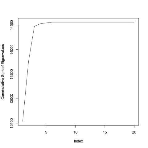
Figure 3: Cumulative Sums for the Polynomial Kernel.

3.3 Numerical Approximations of Eigenvalues and Eigenvectors

The pseudo-inverse only involves the first $k$ largest eigenvalues and eigenvectors that need to be numerically obtained when $n$ is so large that the kernel matrix is ill-conditioned. Numerical methods have been developed to approximate these eigen-terms to any desired precision, which include the random projection method through the Johnson-Lindenstrauss transformation (Sarlos, 2006; Halko et al., 2011; Banerjee et al., 2013), the Nyström method (Drineas and Mahoney, 2005), the Block Lanczos Method (Cullum and Donath, 1974; Golub and Underwood, 1977), and the Block Krylov Iteration Method (Musco and Musco, 2015). These algorithms are able to approximate the eigenvalues and eigenvectors of an extremely large $n\times n$ matrix $V$ and can be programmed to run quite efficiently.

3.4 The Pseudo-inverse versus the Perturbation Approach

The optimal rank-$k$ approximation to the covariance matrix $V_{n}$ is obviously rank deficient if $k<n$. Theorem 2 shows that the pseudo-inverse can be used for spatial prediction and compares the resulting prediction variance to the exact kriging variance. A more common practice, though, is to add a perturbation term $\tau I_{n}$ to the low-rank approximation (Williams and Seeger, 2000). There are two situations where such a perturbation is warranted. One is when the data contain measurement error or the covariance function has a nugget effect. Another is when the Representer Theorem applies, so that the $\tau$ term represents regularization (Wahba, 2002).

However, the nugget effect is not always present, as in some studies in computer experiments that usually use nuggetless covariance functions (e.g. Kennedy and O’Hagan, 2001; Rasmussen and Williams, 2006), oceanography (Long, 2021; Jacobs et al., 2001), and climatology (Xu and Gong, 2003), among other areas. Suppose the covariance function has no nugget effect and a perturbation term is added to the rank-$k$ approximation to increase the numerical stability. Then the kriging coefficient $\alpha$ in (12) is now a solution to

$$(V_{n,k}+\tau I_{n})\mbox{\boldmath$\alpha$}(s)=\mbox{\boldmath$k$}(s)$$

where $V_{n,k}=\sum_{i=1}^{k}\lambda_{n,i}\mbox{\boldmath$u$}_{i}\mbox{\boldmath$u$}_{i}^{\prime}$ is the rank-$k$ approximation to $V_{n}$. The interpolated value of $Y$ is

$$\hat{}\mbox{\boldmath$Y$}=V_{n}(V_{n,k}+\tau I_{n})^{-1}\mbox{\boldmath$Y$}.$$

We can show that

$$E\|\mbox{\boldmath$Y$}-\hat{}\mbox{\boldmath$Y$}\|^{2}=\sum_{i=1}^{k}\frac{\lambda_{n,i}}{(1+\lambda_{n,i}/\tau)^{2}}+\sum_{i>k}\lambda_{n,i}(1-\lambda_{n,i}/\tau)^{2}.$$ (14)

The first term is strictly increasing in $\tau$ and falls within the interval $(0,\sum_{i=1}^{k}\lambda_{n,i})$. However, the second term decreases for $\tau<\sum_{i>k}\lambda_{i}^{3}/\sum_{i>k}\lambda_{i}^{2}<\lambda_{n,k+1}$, and then starts to increase. Consequently, the chosen $\tau$ should be less than $\lambda_{n,k+1}$ in order to minimize the sum of mean square errors. Nevertheless, the second term can become quite large for a very small $\tau$. Therefore, as we increase $\tau$ to enhance numerical stability, we might risk increasing the mean square error of prediction.

For pseudo kriging with $k$ eigenvalues, the sum of mean squared errors at the $n$ locations is $\sum_{i>k}\lambda_{n,i}$ (See Theorem 4 in the next section). We now compare it that of the perturbation method through an example. Consider the same setting as in the previous section, with the covariance function chosen to be the Gaussian $K_{3}$. We set $k=100$ and obtain $\sum_{i>k}\lambda_{n,i}=2.834\times 10^{-4}$. We calculate the sum of MSE in (14) for four different values of $\tau$ and the corresponding condition number. Results are reported in Table 1. Therefore, $\tau$ must be smaller than 0.001 in order to achieve a sum of MSE comparable to that of the pseudo-inverse method. The resulting matrix will be more ill-conditioned than when $\tau=0.001$.

Table 1: Condition Numbers and Sum of MSE for the Perturbation Method

	$\tau$	Condition Number	$E\|\mbox{\boldmath$Y$}-\hat{}\mbox{\boldmath$Y$}\|^{2}$
1	0.0010	1141758.43	0.006737
2	0.0100	114175.84	0.063977
3	0.1000	11417.58	0.602860
4	1.0000	1141.76	5.618669

4 Optimal Low-Rank Approximation

Theorem 1 suggests that as $n$ increases, the covariance matrix becomes ill-conditioned, provided the sampling locations are not distributed too unevenly. This ill-conditioning issue is not limited to regular covariance matrices; it also affects tapered covariance matrices because the theorem applies to them as well. Low-rank models have been developed to address this ill-conditioning problem, and the main theorem lends further support to the use of such models. However, given the myriad of low-rank models available in the literature, it’s crucial to establish criteria for selecting appropriate low-rank approximations. This section delves into that exact topic.

In this section, we explore various criteria for low-rank approximations and present the optimal solution corresponding to each criterion. Notably, these optimal solutions may not always align with what we aim to achieve in practice. Instead, they epitomize the best possible outcomes under certain conditions. Interestingly, the findings from this section will play a role in the proof for Theorem 1.

We begin by defining the low-rank approximation of a stochastic process, distinguishing it from the low-rank models used for high-dimensional data, such as principal component analysis (PCA). For a second-order process $Y(s)$ with a continuous covariance function and mean 0, a low-rank approximation is given by:

$$Y^{*}(s)=\sum_{i=1}^{k}a_{i}(s)Z_{i}.$$

Here, $Z_{i}$ for $i=1,2,...,k$ represents a set of uncorrelated random variables with unit variance, while $a_{i}(s)$ for $i=1,2,...,k$ signifies real functions. Such a process is termed a rank-$k$ approximation. For a specified $k$, we assess the optimal rank-$k$ process that approximates the intrinsic process $Y(s),s\in D$. We delve into three methods to define this optimality.

Optimality A

To minimize

$$\int_{D}E\left(Y(s)-\sum_{i=1}^{k}a_{i}(s)Z_{i}\right)^{2}ds$$

over all functions real and square integrable functions $a_{i}(s)$ (i.e., $\int_{D}a_{i}^{2}(s)ds<\infty$) and all random variables $Z_{i}$.

We note that Optimality A is equivalent to

$$\min_{W_{k}}\int_{D}E\left(Y(s)-\Pi[Y(s)|W_{k}]\right)^{2}ds$$

where the minimum is over all $k$-dimensional subspace $W_{k}$ in $H$. The subspace $W_{k}$ that reaches the minimum is called the optimal subspace. The optimal subspace is spanned by the first $k$ eigenfunctions as shown in (4).

Optimality B

To minimize

$$\int_{D}E\left(Y(s)-\sum_{i=1}^{k}a_{i}(s)Z_{i}\right)^{2}ds$$

over all real and square integrable functions $a_{i}(s)$ and all $Z_{j}\in H_{n}=\text{span}\{Y(s_{i}),~{}i=1,,2\ldots,n\}$.

It is equivalent to minimizing

$$\int_{D}E\left(Y(s)-\Pi[Y(s)|S_{k}]\right)^{2}ds$$

over all $k$-dimensional subspaces $S_{k}$ in $H_{n}=\text{span}\{Y(s_{i}),~{}i=1,,2\ldots,n\}$. The optimal solution will be provided in Theorem 3.

Optimality C

To minimize

$$\sum_{i=1}^{n}E\left(Y(s_{i})-\sum_{j=1}^{k}a_{ij}Z_{j}\right)^{2}$$

over all constants $a_{ij}$ and $k$ random variables $Z_{1},Z_{2},\ldots,Z_{k}$ that are linearly independent.

The last criterion is equivalent to minimizing

$$\sum_{i=1}^{n}E\left(Y(s_{i})-\Pi[Y(s_{i})|S_{k}]\right)^{2}$$

over all $k$-dimensional subspaces $S_{k}$ in $H_{n}$. This criterion only concerns the process at the sampling locations $s_{i}$. The optimal solution will be provided in Theorem 4.

Since the optimal solution under Optimality A is known to be the truncated KL expansion, we will focus on the optimal low-rank approximations under the other two criteria.

For the underlying process $Y(s),s\in D$, define the Kriging predictor

$$Y_{n}^{*}(s)=\Pi[Y(s)|Y(s_{1}),Y(s_{2}),\ldots,Y(s_{n})].$$

Banerjee et al. (2008) called $Y_{n}^{*}(s)$ the predictive process. It turns out the the optimal solution under Optimality B can be given through the predictive process. First, we note the predictive process has a continuous covariance function when $K(s,x)$ is continuous. Hence $Y_{n}^{*}(s)$ has the Karhunen-Loéve expansion

$$Y_{n}^{*}(s)=\sum_{i=1}^{n}\sqrt{\lambda_{n,i}^{*}}\varphi_{n,i}^{*}(s)Z_{ni}$$ (15)

where the functions $\varphi_{n,i}^{*}(s)$ satisfy $\int_{D}\varphi_{n,i}^{*}(s)\varphi_{n,j}^{*}(s)ds=\delta_{ij}$, and $Z_{ni}$ are a set of uncorrelated random variables with the unit variance. Note these $Z_{n,i}$’s generally are not in the space $H_{n}$.

Theorem 3

For $1\leq k<n$,

$$\min_{W_{k}}\int_{D}E\left(Y(s)-\Pi[Y(s)|W_{k}]\right)^{2}ds=\sum_{i=k+1}^{n}\lambda_{n,i}^{*}+\int_{D}E(Y(s)-Y_{n}^{*}(s))^{2}ds$$ (16)

where the minimum is over $k$-dimensional subspace $W_{k}$ in $H_{n}$. The optimal subspace is $W_{k}=\mbox{span}\{Z_{ni}^{*},i=1,2,\ldots,k\}$ and the optimal solution under Optimality B is $\sum_{i=1}^{k}\sqrt{\lambda_{n,i}^{*}}\varphi_{n,i}^{*}(s)Z_{ni}^{*}$, where $\lambda_{n,i}^{*}$, $\varphi_{n,i}^{*}$ and $Z_{n,i}^{*}$ are defined by (15).

The following theorem follows results in Algazi and Sakrison (1969) and Dür (1998) and provides the solution under Optimality C.

Theorem 4

Let $\lambda_{n,i}$ denote the $i$th eigenvalue of $V_{n}$, $i=1,2,\ldots,n$. Then for any $k$-dimensional subspace $W_{k}\subset H$,

$$\min_{W_{k}}\sum_{i=1}^{n}\text{E}(Y(s_{i})-\Pi[Y(s_{i})|W_{k}])^{2}=\sum_{i=k+1}^{n}\lambda_{n,i}.$$

The minimum is reached when $W_{k}=\text{span}\{\mbox{\boldmath$u$}_{i}^{\prime}\mbox{\boldmath$Y$},i=1,2,\ldots,k\}$ where $\mbox{\boldmath$u$}_{i}$ is the eigenvector of $V_{n}$ corresponding to the eivenvalue $\lambda_{n,i}$.

5 Concluding Remarks

We have shown that as the sample size $n$ increases, the kernel matrix tends to be ill-conditioned, provided the sampling locations are not overly dispersed. This ill-conditioning introduces numerical instability in computations related to prediction and the Gaussian likelihood. As a result, numerical approximations become imperative for the kernel matrix and its inverse.

This discovery motivates further exploration of methodologies tailored for handling extensive spatial datasets. While some techniques, like covariance tapering, fail to address the ill-conditioning problem, others, such as the low-rank approximation, prove to be effective in resolving the issue.

Such findings pave the way for intriguing questions yet to be addressed. For instance, when one employs approximations on the kernel matrix to mitigate ill-conditioning, how does this modification influence the Gaussian likelihood function? Furthermore, what ramifications does this have on the maximum likelihood estimation? We posit that these questions may be addressed through methodologies similar to those presented in Tang et al. (2021).

6 Appendix

We will first prove Theorem 3 because the proof of Theorem 1 depends on Theorem 3.

Proof of Theorem 3. Since $W_{k}\subset H_{n}$,

$$E\left(Y(s)-\Pi[Y(s)|W_{k}]\right)^{2}=E\left(Y(s)-Y_{n}^{*}(s)\right)^{2}+E\left(Y^{*}(s)-\Pi[Y_{n}^{*}(s)|W_{k}]\right)^{2}.$$

It follows

$$\int_{D}E\left(Y(s)-\Pi[Y(s)|W_{k}]\right)^{2}ds$$

$$=\int_{D}E\left(Y(s)-Y_{n}^{*}(s)\right)^{2}ds+\int_{D}E\left(Y_{n}^{*}(s)-\Pi[Y_{n}^{*}(s)|W_{k}]\right)^{2}ds.$$

The first term in the right hand does not depend on $W_{k}$, and the second term is minimized when $W_{k}=span\{Z_{n,i},i=1,2,\ldots,k\}$, and the minimum is $\sum_{i>k}\lambda_{n,i}^{*}$ by (4). Theorem 3 is proved.

Theorem 1 is proved by taking $W_{k}=\text{span}\{Z_{ni},i=1,2,\ldots,k\}$ in both Theorems 3 and 4 and comparing the two minimums. Intuitively, if $\Omega$ is a small area and $s_{0}\in\Omega$,

$$|\Omega|E(Y(s_{0})-\Pi(Y(s_{0})|W))^{2}\approx\int_{\Omega}E(Y(s)-\Pi[Y(s)|W])^{2}ds.$$

The following lemma formally establishes the relationship. First, define

$$c(\delta)=\inf\{(K(x_{1},x_{2})/K(x_{2},x_{2}))^{2}:\|x_{1}-x_{2}\|\leq\delta,x_{1},x_{2}\in D\}.$$ (17)

The uniform continuity of $K$ implies that $c(\delta)\to 1$ when $\delta\to 0$.

Lemma 1

Let $\Omega\subset D$ and $s_{0}$ be a point in $\Omega$. Then for any subspace $W\subset H$,

$$(1/2)\int_{\Omega}E(Y(s)-\Pi[Y(s)|W])^{2}ds-(1-c(\delta))\int_{\Omega}K(s,s)ds$$

$$\leq c(\delta)|\Omega|E(Y(s_{0})-\Pi(Y(s_{0})|W))^{2}$$ (18)

$$\leq 2\int_{\Omega}E(Y(s)-\Pi[Y(s)|W])^{2}ds+2(1-c(\delta))\int_{\Omega}K(s,s)ds$$ (19)

where $\delta=\Delta(\Omega)$.

Proof of Lemma 1. We regress $Y(s)$ on $Y(s_{0})$ to get

$$Y(s)=\rho(s)Y(s_{0})+\epsilon(s)$$

where $\rho(s)=K(s,s_{0})/K(s_{0},s_{0})$, and

$$E(\epsilon(s)^{2})=E(Y(s)^{2})-\rho(s)^{2}E(Y(s_{0})^{2})\\ =K(s,s)-K(s,s_{0})^{2}/K(s_{0},s_{0}).$$

It follows that

$$E\epsilon(s)^{2}\leq K(s,s)(1-c(\delta)).$$ (20)

Then for any subspace $W$

$$Y(s)-\Pi[Y(s)|W]$$

$$=\rho(s)(Y(s_{0})-\Pi[Y(s_{0})|W])+(\epsilon(s)-\Pi[\epsilon(s)|W]).$$ (21)

The inequality $E(X+Y)^{2}\leq 2(EX^{2}+EY^{2})$ for any random variables $X$ and $Y$ implies

$$\rho(s)^{2}E(Y(s_{0})-\Pi(Y(s_{0})|W))^{2}$$

$$\leq 2E(Y(s)-\Pi(Y(s)|W))^{2}+2E(\epsilon(s))^{2},\mbox{ for any }s\in\Omega.$$ (22)

This inequality and (20) imply

$$\left(\int_{\Omega}\rho(s)^{2}ds\right)E(Y(s_{0})-\Pi(Y(s_{0})|W))^{2}$$

$$\leq 2\int_{\Omega}E(Y(s)-\Pi(Y(s)|W))^{2}+2(1-c(\delta))\int_{D}K(s,s)ds.$$

The inequality (19) follows because $\rho(s)^{2}\geq c(\delta)$. Equation (18) can be proved similarly by applying the inequality $E(X^{2})\geq(1/2)E(X-Y)^{2}-E(Y^{2})$ for any two random variables $X$ and $Y$ to Eq. (21).

Lemma 2

Let $\lambda_{n,i}^{*}$ be the eigenvalues in (15) and $\lambda_{i}$ the eigenvalue in (1). For any $i\leq n$, $\lambda_{n,i}^{*}\leq\lambda_{i}$.

Proof. The Lemma follows Proposition 5 in Santin and Schaback (2016).

Proof of Theorem 1. For simplicity, we suppress $n$ in $D_{n,i}$ and other notations when no confusions arise. Define $\delta_{i}=\Delta(D_{i})$. By Lemma 1,

$$c(\delta_{i})|D_{i}|E(Y(s_{i})-\Pi(Y(s_{i})|W_{k}))^{2}$$

$$\leq 2\int_{D_{i}}E(Y(s)-\Pi[Y(s)|W_{k}])^{2}ds+(1-c(\delta_{i}))\int_{D_{i}}K(s,s)ds.$$ (23)

Since $|D|=\sum_{i=1}^{n}|D_{i}|\leq n\max|D_{i}|\leq n\gamma\min_{i}|D_{i}|,$ we get

$$\min_{i}|D_{i}|\geq|D|/(n\gamma).$$

Using the last inequality and adding up both sides of (23), we see

$$\min_{i}c(\delta_{i})(n\gamma)^{-1}|D|\sum_{i=1}^{n}E(Y(s_{i})-\Pi(Y(s_{i})|W_{k}))^{2}$$

$$\leq 2\int_{D}E(Y(s)-\Pi[Y(s)|W_{k}])^{2}ds+(1-\min_{i}c(\delta_{i}))\int_{D}K(s,s)ds$$

The inequality is true for any $k$-dimensional space $W_{k}$. In particular, taking $W_{k}$ to the be optimal subspace in Theorem 3 and applying Theorem 4, we have

$$\min_{i}c(\delta_{i})(n\gamma)^{-1}|D|\sum_{i>k}\lambda_{n,i} \leq 2\left(\sum_{i=k+1}^{n}\lambda_{n,i}^{*}+\int_{D}E(Y(s)-Y_{n}^{*}(s))^{2}ds\right)$$

$$+(1-\min_{i}c(\delta_{i}))\int_{D}K(s,s)ds$$

$$\leq 2\left(\sum_{i>k}\lambda_{i}+\int_{D}E(Y(s)-Y_{n}^{*}(s))^{2}ds\right)$$

$$+(1-\min_{i}c(\delta_{i}))\int_{D}K(s,s)ds.$$

The last inequality follows Lemma 2. Let us bound the integral now.

$$\int_{D}E(Y(s)-Y_{n}^{*}(s))^{2}ds=\sum_{i=1}^{n}\int_{D_{i}}E(Y(s)-Y_{n}^{*}(s))^{2}ds$$ (24)

$$\leq\sum_{i=1}^{n}\int_{D_{i}}E(Y(s)-\Pi[Y(s)|Y(s_{i})])^{2}ds.$$ (25)

Applying (21), for $s\in D_{i}$, we get

$$E(Y(s)-\Pi[Y(s)|Y(s_{i})])^{2}\leq K(s_{i},s_{i})(1-c(\delta_{i})).$$

It follows

$$\int_{D}E(Y(s)-Y_{n}^{*}(s))^{2}ds\leq|D|(1-\min_{i}c(\delta_{i}))\max_{s\in D}K(s,s).$$

We have established

$$\min_{i}c(\delta_{i})(n\gamma)^{-1}|D|\sum_{i>k}\lambda_{n,i}\leq 2\sum_{i>k}\lambda_{i}+(1+|D|)(1-\min_{i}c(\delta_{i}))\max_{s\in D}K(s,s).$$

The theorem follows.

Proof of Corollary 1. From (9), it is seen that $\lim_{k\to\infty}\sum_{i>k}\lambda_{n,i}/n\to 0$. Therefore for any $i\leq n$ and $i\to\infty$, $\lambda_{n,i}/n\to 0$. The corollary holds if $\liminf_{n\to\infty}\lambda_{n,1}/n>0$. Therefore, it suffices to show

$$\lambda_{n,1}/n\geq a\lambda_{1}+o(1)\mbox{ as }n\to\infty.$$ (26)

To that end, we first observe that Mercer’s Theorem (2) implies

$$\lambda_{1}=\int_{D}\int_{D}\phi_{1}(x)K(x,y)\phi_{1}(y)dxdy.$$

The continuity of the integrant implies that the integral can be approximated by a finite sum, i.e.,

$$\lambda_{1}=\sum_{i=1}^{n}\sum_{j=1}^{n}|D_{i}||D_{j}|\phi_{1}(s_{i})\phi_{1}(s_{j})K(s_{i},s_{j})+o(1)$$

Similarly,

$$1=\int_{D}\phi_{1}^{2}(x)dx=\sum_{i=1}^{n}|D_{i}|\phi_{1}^{2}(s_{i})+o(1)$$

It follows the last equations that

$$\lambda_{1}=\frac{\sum_{i=1}^{n}\sum_{j=1}^{n}|D_{i}||D_{j}|\phi_{1}(s_{i})\phi_{1}(s_{j})K(s_{i},s_{j})}{\sum_{i=1}^{n}|D_{i}|\phi_{1}^{2}(s_{i})}+o(1).$$ (27)

As we previously established, $\min_{i}|D_{i}|\geq|D|/(rn)$. Then

Then, from (27),

$$\lambda_{1} \leq\frac{|D|}{rn}\frac{\sum_{i=1}^{n}\sum_{j=1}^{n}|D_{i}||D_{j}|\phi_{1}(s_{i})\phi_{1}(s_{j})K(s_{i},s_{j})}{\sum_{i=1}^{n}D_{i}^{2}\phi_{1}^{2}(s_{i})}+o(1)$$

$$\leq\frac{|D|}{rn}\max_{(x_{1},x_{2},\ldots,x_{n})\in R^{n}}\frac{\sum_{i=1}^{n}\sum_{j=1}^{n}x_{i}x_{j}K(s_{i},s_{j})}{\sum_{i=1}^{n}x_{i}^{2}}+o(1)$$

$$=\frac{|D|}{rn}\lambda_{n,1}+o(1).$$

Then (26) immediately follows. The corollary is proved.

Proof of Equation (14). First, note the matrix $V_{n,k}+\tau I_{n}$ has eigenvalues $w_{i}=\lambda_{n,i}+\tau$ for $i\leq k$ and $w_{i}=\tau$ for $i>k$, and shares the same eigenvectors $\mbox{\boldmath$u$}_{i}$ with $V_{n}$. Then

$$(V_{n,k}+\tau I_{n})^{-1}=\sum_{i=1}^{n}w_{i}^{-1}\mbox{\boldmath$u$}_{i}\mbox{\boldmath$u$}_{i}^{\prime}$$

$$V_{n}(V_{n,k}+\tau I_{n})^{-1}=\sum_{i=1}^{n}\lambda_{n,i}w_{i}^{-1}\mbox{\boldmath$u$}_{i}\mbox{\boldmath$u$}_{i}^{\prime}.$$

Hence $\hat{}\mbox{\boldmath$Y$}=\sum_{i=1}^{n}\lambda_{n,i}w_{i}^{-1}Z_{i}\mbox{\boldmath$u$}_{i}$ for $Z_{i}=\mbox{\boldmath$u$}_{i}^{\prime}\mbox{\boldmath$Y$}$. Applying (5) to get

$$\mbox{\boldmath$Y$}-\hat{}\mbox{\boldmath$Y$}=\sum_{i=1}^{n}(1-\lambda_{n,i}w_{i}^{-1})Z_{i}\mbox{\boldmath$u$}_{i}$$

and

$$\|\mbox{\boldmath$Y$}-\hat{}\mbox{\boldmath$Y$}\|^{2}=\sum_{i=1}^{n}(1-\lambda_{n,i}w_{i}^{-1})^{2}Z_{i}^{2}.$$

Equation (14) is proved by observing $EZ_{i}^{2}=\lambda_{n,i}$ and $Z_{i}$’s are uncorrelated.

References

- Algazi and Sakrison (1969) Algazi, V. and Sakrison, D. (1969) On the optimality of the Karhunen-Loève expansion (Corresp.). IEEE Transactions on Information Theory, 15, 319–321.
- Bagnell et al. (2009) Bagnell, J. A., Bradley, D. and Hebert, M. (2009) Kernel methods in computer vision. Foundations and Trends in Computer Graphics and Vision, 4, 1–196. Publisher: Now Publishers Inc.
- Banerjee et al. (2013) Banerjee, A., Dunson, D. B. and Tokdar, S. T. (2013) Efficient Gaussian process regression for large datasets. Biometrika, 100, 75–89. URL: http://www.jstor.org/stable/43304538. Publisher: [Oxford University Press, Biometrika Trust].
- Banerjee et al. (2008) Banerjee, S., Gelfand, A. E., Finley, A. O. and Sang, H. (2008) Gaussian predictive process models for large spatial data sets. Journal of the Royal Statistical Society: Series B (Statistical Methodology), 70, 825–848. URL: https://onlinelibrary.wiley.com/doi/abs/10.1111/j.1467-9868.2008.00663.x. _eprint: https://onlinelibrary.wiley.com/doi/pdf/10.1111/j.1467-9868.2008.00663.x.
- Belkin (2018) Belkin, M. (2018) Approximation beats concentration? An approximation view on inference with smooth radial kernels. Proceedings of Machine Learning Research, 75, 1–14.
- Belkin et al. (2019) Belkin, M., Rakhlin, A. and Tsybakov, A. B. (2019) Does data interpolation contradict statistical optimality? In Proceedings of the Twenty-Second International Conference on Artificial Intelligence and Statistics (eds. K. Chaudhuri and M. Sugiyama), vol. 89 of Proceedings of Machine Learning Research, 1611–1619. PMLR. URL: https://proceedings.mlr.press/v89/belkin19a.html.
- Bradley et al. (2016) Bradley, J. R., Cressie, N. and Shi, T. (2016) A comparison of spatial predictors when datasets could be very large. Statistics Surveys, 10, 100–131. Publisher: Amer. Statist. Assoc., the Bernoulli Soc., the Inst. Math. Statist., and the Statist. Soc. Canada.
- Braun (2006) Braun, M. L. (2006) Accurate Error Bounds for the Eigenvalues of the Kernel Matrix. Journal of Machine Learning Research, 7, 2303–2328. URL: http://jmlr.org/papers/v7/braun06a.html.
- Cressie and Johannesson (2008) Cressie, N. and Johannesson, G. (2008) Fixed rank kriging for very large spatial data sets. Journal of the Royal Statistical Society: Series B (Statistical Methodology), 70, 209–226. Publisher: Wiley.
- Cullum and Donath (1974) Cullum, J. and Donath, W. E. (1974) A block Lanczos algorithm for computing the q algebraically largest eigenvalues and a corresponding eigenspace of large, sparse, real symmetric matrices. In IEEE Conference on Decision and Control including the 13th Symposium on Adaptive Processes, 505–509.
- Currin et al. (1991) Currin, C., Mitchell, T., Morris, M. and Ylvisaker, D. (1991) Bayesian Prediction of Deterministic Functions, with Applications to the Design and Analysis of Computer Experiments. Journal of the American Statistical Association, 86, 953–963. URL: https://www.jstor.org/stable/2290511.
- Datta (2021) Datta, A. (2021) Sparse nearest neighbor Cholesky matrices in spatial statistics. URL: http://arxiv.org/abs/2102.13299. ArXiv:2102.13299 [stat].
- Datta (2022) — (2022) Nearest-neighbor sparse Cholesky matrices in spatial statistics. WIREs Computational Statistics, 14, e1574. URL: https://onlinelibrary.wiley.com/doi/abs/10.1002/wics.1574. _eprint: https://onlinelibrary.wiley.com/doi/pdf/10.1002/wics.1574.
- Datta et al. (2016a) Datta, A., Banerjee, S., Finley, A. O. and Gelfand, A. E. (2016a) Hierarchical Nearest-Neighbor Gaussian Process Models for Large Geostatistical Datasets. Journal of the American Statistical Association, 111, 800–812. URL: https://doi.org/10.1080/01621459.2015.1044091. Publisher: Taylor & Francis _eprint: https://doi.org/10.1080/01621459.2015.1044091.
- Datta et al. (2016b) Datta, A., Banerjee, S., Finley, A. O., Hamm, N. A., Schaap, M. and al, e. (2016b) Nonseparable dynamic nearest neighbor Gaussian process models for large spatio-temporal data with an application to particulate matter analysis. The Annals of Applied Statistics, 10, 1286–1316. Publisher: Institute of Mathematical Statistics.
- Deisenroth et al. (2015) Deisenroth, M. P., Fox, D. and Rasmussen, C. E. (2015) Gaussian Processes for Data-Efficient Learning in Robotics and Control. IEEE Transactions on Pattern Analysis and Machine Intelligence, 37, 408–423. URL: http://arxiv.org/abs/1502.02860. ArXiv:1502.02860 [cs, stat].
- Drineas and Mahoney (2005) Drineas, P. and Mahoney, M. W. (2005) On the Nystrom Method for Approximating a Gram Matrix for Improved Kernel-Based Learning. Journal of Machine Learning Research, 6, 2153–2175.
- Dür (1998) Dür, A. (1998) On the Optimality of the Discrete Karhunen–Loève Expansion. SIAM Journal on Control and Optimization, 36, 1937–1939.
- Du et al. (2009) Du, J., Zhang, H. and Mandrekar, V. S. (2009) Fixed-domain asymptotic properties of tapered maximum likelihood estimators. Annals of Statistics, 37, 3330–3361. Times Cited: 8.
- Eidsvik et al. (2014) Eidsvik, J., Shaby, B. A., Reich, B. J., Wheeler, M. and Niemi, J. (2014) Estimation and prediction in spatial models with block composite likelihoods. Journal of Computational and Graphical Statistics, 23, 295–315. Publisher: Taylor & Francis.
- Finley et al. (2009) Finley, A. O., Sang, H., Banerjee, S. and Gelfand, A. E. (2009) Improving the performance of predictive process modeling for large datasets. Computational Statistics & Data Analysis, 53, 2873–2884. Publisher: Elsevier.
- Furrer et al. (2006) Furrer, R., Genton, M. G. and Nychka, D. (2006) Covariance Tapering for Interpolation of Large Spatial Datasets. Journal of Computational and Graphical Statistics, 15, 502–523. URL: https://doi.org/10.1198/106186006X132178. Publisher: Taylor & Francis _eprint: https://doi.org/10.1198/106186006X132178.
- Ghanem and Spanos (1991) Ghanem, R. G. and Spanos, P. D. (1991) Stochastic Finite Elements: A Spectral Approach. New York: Springer New York.
- Golub and Underwood (1977) Golub, G. and Underwood, R. (1977) The block Lanczos method for computing eigenvalues. Mathematical Software, 3, 361–377.
- Golub and Loan (2012) Golub, G. H. and Loan, C. F. V. (2012) Matrix Computations. Baltimore, Maryland: Johns Hopkins University Press, 4 edn.
- Guinness (2018) Guinness, J. (2018) Permutation and Grouping Methods for Sharpening Gaussian Process Approximations. Technometrics, 60, 415–429. URL: https://doi.org/10.1080/00401706.2018.1437476. Publisher: Taylor & Francis _eprint: https://doi.org/10.1080/00401706.2018.1437476.
- Halko et al. (2011) Halko, N., Martinsson, P. G. and Tropp, J. A. (2011) Finding Structure with Randomness: Probabilistic Algorithms for Constructing Approximate Matrix Decompositions. SIAM Review, 53, 217–288. URL: https://doi.org/10.1137/090771806. _eprint: https://doi.org/10.1137/090771806.
- Heaton et al. (2019) Heaton, M. J., Datta, A., Finley, A. O., Furrer, R., Guinness, J., Guhaniyogi, R., Gerber, F., Gramacy, R. B., Hammerling, D., Katzfuss, M., Lindgren, F., Nychka, D. W., Sun, F. and Zammit-Mangion, A. (2019) A Case Study Competition Among Methods for Analyzing Large Spatial Data. Journal of Agricultural, Biological and Environmental Statistics, 24, 398–425. URL: https://doi.org/10.1007/s13253-018-00348-w.
- Higdon (2002) Higdon, D. (2002) Space and Space-Time Modeling using Process Convolutions. In Quantitative Methods for Current Environmental Issues (eds. C. W. Anderson, V. Barnett, P. C. Chatwin and A. H. El-Shaarawi), 37–56. London: Springer.
- Jacobs et al. (2001) Jacobs, G. A., Barron, C. N. and Rhodes, R. C. (2001) Mesoscale characteristics. Journal of Geophysical Research: Oceans, 106, 19581–19595. URL: https://doi.org/10.1029/2000JC000669. Publisher: John Wiley & Sons, Ltd.
- Jia and Liao (2009) Jia, L. and Liao, S. (2009) Accurate Probabilistic Error Bound for Eigenvalues of Kernel Matrix. In Advances in Machine Learning (eds. Z.-H. Zhou and T. Washio), 162–175. Berlin, Heidelberg: Springer Berlin Heidelberg.
- Kang and Cressie (2011) Kang, E. L. and Cressie, N. (2011) Bayesian inference for the spatial random effects model. Journal of the American Statistical Association, 106, 972–983. Publisher: Taylor & Francis.
- Katzfuss and Cressie (2011) Katzfuss, M. and Cressie, N. (2011) Spatio-temporal smoothing and EM estimation for massive remote-sensing data sets. Journal of Time Series Analysis, 32, 430–446. Publisher: Wiley Online Library.
- Kaufman et al. (2008) Kaufman, C. G., Schervish, M. J. and Nychka, D. W. (2008) Covariance tapering for likelihood-based estimation in large spatial data sets. Journal of the American Statistical Association, 103, 1545–1555. Publisher: Taylor & Francis.
- Kennedy and O’Hagan (2001) Kennedy, M. C. and O’Hagan, A. (2001) Bayesian Calibration of Computer Models. Journal of the Royal Statistical Society Series B: Statistical Methodology, 63, 425–464. URL: https://doi.org/10.1111/1467-9868.00294.
- Koltchinskii and Giné (2000) Koltchinskii, V. and Giné, E. (2000) Random matrix approximation of spectra of integral operators. Bernoulli, 6, 113–167. URL: https://projecteuclid.org/journals/bernoulli/volume-6/issue-1/Random-matrix-approximation-of-spectra-of-integral-operators/bj/1082665383.full. Publisher: Bernoulli Society for Mathematical Statistics and Probability.
- König (1986) König, H. (1986) Eigenvalue Distribution of Compact Operators, vol. 16 of Operator Theory: Advances and Applications. Basel: Birkhäuser Verlag.
- Lemos and Sansó (2009) Lemos, R. T. and Sansó, B. (2009) A spatio-temporal model for mean, anomaly, and trend fields of North Atlantic sea surface temperature. Journal of the American Statistical Association, 104, 5–18. Publisher: Taylor & Francis.
- Lindgren et al. (2011) Lindgren, F., Rue, H. and Lindström, J. (2011) An explicit link between Gaussian fields and Gaussian Markov random fields: the stochastic partial differential equation approach. Journal of the Royal Statistical Society: Series B (Statistical Methodology), 73, 423–498. URL: https://onlinelibrary.wiley.com/doi/abs/10.1111/j.1467-9868.2011.00777.x.
- Long (2021) Long, M. H. (2021) Aquatic Biogeochemical Eddy Covariance Fluxes in the Presence of Waves. Journal of Geophysical Research: Oceans, 126, e2020JC016637. URL: https://doi.org/10.1029/2020JC016637. Publisher: John Wiley & Sons, Ltd.
- Musco and Musco (2015) Musco, C. and Musco, C. (2015) Randomized Block Krylov Methods for Stronger and Faster Approximate Singular Value Decomposition. In Advances in Neural Information Processing Systems (eds. C. Cortes, N. Lawrence, D. Lee, M. Sugiyama and R. Garnett), vol. 28. Curran Associates, Inc. URL: https://proceedings.neurips.cc/paper/2015/file/1efa39bcaec6f3900149160693694536-Paper.pdf.
- Nychka et al. (2015) Nychka, D., Bandyopadhyay, S., Hammerling, D., Lindgren, F. and Sain, S. (2015) A Multiresolution Gaussian Process Model for the Analysis of Large Spatial Datasets. Journal of Computational and Graphical Statistics, 24, 579–599. URL: http://www.jstor.org/stable/24737282. Publisher: [American Statistical Association, Taylor & Francis, Ltd., Institute of Mathematical Statistics, Interface Foundation of America].
- O’Hagan (1978) O’Hagan, A. (1978) Curve fitting and optimal design for predictions. Journal of the Royal Statistical Society B, 40, 1–42.
- Pietsch (1987) Pietsch, A. (1987) Eigenvalues and s-Numbers, vol. 13 of Cambridge Studies in Advanced Mathematics. Cambridge: Cambridge University Press.
- Rasmussen and Williams (2006) Rasmussen, C. E. and Williams, C. K. I. (2006) Gaussian Processes for Machine Learning. MIT Press. URL: http://www.gaussianprocess.org/gpml/.
- Raykar and Duraiswami (2007) Raykar, V. C. and Duraiswami, R. (2007) Kernel methods in signal processing. Signal Processing Magazine, IEEE, 24, 118–121. Publisher: IEEE.
- Rue et al. (2009) Rue, H., Martino, S. and Chopin, N. (2009) Approximate Bayesian inference for latent Gaussian models by using integrated nested Laplace approximations. Journal of the Royal Statistical Society: Series B (Statistical Methodology), 71, 319–392. Publisher: Wiley Online Library.
- Santin and Schaback (2016) Santin, G. and Schaback, R. (2016) Approximation of eigenfunctions in kernel-based spaces. Advances in Computational Mathematics, 42, 973–993. URL: https://doi.org/10.1007/s10444-015-9449-5.
- Sarlos (2006) Sarlos, T. (2006) Improved Approximation Algorithms for Large Matrices via Random Projections. In 2006 47th Annual IEEE Symposium on Foundations of Computer Science (FOCS’06), 143–152. ISSN: 0272-5428.
- Schaback (1995) Schaback, R. (1995) Error estimates and condition numbers for radial basis function interpolation. Advances in Computational Mathematics, 3, 251–264. URL: https://doi.org/10.1007/BF02432002.
- Schaback and Wendland (2002) Schaback, R. and Wendland, H. (2002) Approximation by positive definite kernels. In Advanced Problems in Constructive Approximation (eds. M. D. Buhmann and D. H. Mache), 203–222. Basel: Birkhäuser Basel.
- Schölkopf and Smola (2002) Schölkopf, B. and Smola, A. J. (2002) Learning with Kernels. Cambridge, MA: MIT Press.
- Schölkopf et al. (2004) Schölkopf, B., Tsuda, K. and Vert, J.-P. (eds.) (2004) Kernel methods in computational biology. MIT Press.
- Shawe-Taylor and Cristianini (2004) Shawe-Taylor, J. and Cristianini, N. (2004) Kernel methods for pattern analysis. Cambridge University Press.
- Stein (2014) Stein, M. L. (2014) Limitations on low rank approximations for covariance matrices of spatial data. Spatial Statistics, 8, 1–19. URL: https://www.sciencedirect.com/science/article/pii/S2211675313000390.
- Stein et al. (2013) Stein, M. L., Chen, J., Anitescu, M. and al, e. (2013) Stochastic approximation of score functions for Gaussian processes. The Annals of Applied Statistics, 7, 1162–1191. Publisher: Institute of Mathematical Statistics.
- Stein et al. (2004) Stein, M. L., Chi, Z. and Welty, L. J. (2004) Approximating likelihoods for large spatial data sets. Journal of the Royal Statistical Society: Series B (Statistical Methodology), 66, 275–296. Publisher: Wiley.
- Stroud et al. (2017) Stroud, J. R., Stein, M. L. and Lysen, S. (2017) Bayesian and Maximum Likelihood Estimation for Gaussian Processes on an Incomplete Lattice. Journal of Computational and Graphical Statistics, 26, 108–120. URL: https://doi.org/10.1080/10618600.2016.1152970. Publisher: Taylor & Francis _eprint: https://doi.org/10.1080/10618600.2016.1152970.
- Sun et al. (2012) Sun, Y., Li, B. and Genton, M. G. (2012) Geostatistics for Large Datasets. In Advances and Challenges in Space-time Modelling of Natural Events (eds. E. Porcu, J. Montero and M. Schlather), Lecture Notes in Statistics, 55–77. Berlin, Heidelberg: Springer.
- Tang et al. (2021) Tang, W., Zhang, L. and Banerjee, S. (2021) On identifiability and consistency of the nugget in Gaussian spatial process models. Journal of the Royal Statistical Society: Series B (Statistical Methodology), 83, 1044–1070. URL: https://onlinelibrary.wiley.com/doi/abs/10.1111/rssb.12472. _eprint: https://onlinelibrary.wiley.com/doi/pdf/10.1111/rssb.12472.
- Wahba (2002) Wahba, G. (2002) Soft and hard classification by reproducing kernel Hilbert space methods. Proceedings of the National Academy of Sciences, 99, 16524–16530. URL: https://www.pnas.org/doi/10.1073/pnas.242574899. Publisher: Proceedings of the National Academy of Sciences.
- Wang et al. (2023) Wang, Z., Dahl, G. E., Swersky, K., Lee, C., Nado, Z., Gilmer, J., Snoek, J. and Ghahramani, Z. (2023) Pre-trained Gaussian processes for Bayesian optimization. URL: http://arxiv.org/abs/2109.08215. ArXiv:2109.08215 [cs, stat].
- Williams and Seeger (2000) Williams, C. and Seeger, M. (2000) Using the Nyström Method to Speed Up Kernel Machines. In Advances in Neural Information Processing Systems (eds. T. Leen, T. Dietterich and V. Tresp), vol. 13. MIT Press.
- Xu and Gong (2003) Xu, Q. and Gong, J. (2003) Background error covariance functions for Doppler radial-wind analysis. Quarterly Journal of the Royal Meteorological Society, 129, 1703–1720. URL: https://doi.org/10.1256/qj.02.129. Publisher: John Wiley & Sons, Ltd.