Quantifying Interstellar Extinction at High Galactic Latitudes

Abstract

Accurate knowledge of the interstellar medium (ISM) at high Galactic latitudes is crucial for future cosmic microwave background (CMB) polarization experiments due to extinction, albeit low, remaining a foreground larger than the anticipated signal in these regions. We develop a Bayesian model to identify a region of the Hertzsprung-Russell (HR) diagram suited to constrain the single-star extinction accurately at high Galactic latitudes. Using photometry from Gaia, 2MASS and ALLWISE together with parallax from Gaia, we employ nested sampling to fit the model to the data and analyse the posterior over stellar parameters for both synthetic and real data. Charting low variations in extinction is complex due to both systematic errors and degeneracies between extinction and other stellar parameters. The systematic errors can be minimised by restricting our data to a region of the HR diagram where the stellar models are most accurate. Moreover, the degeneracies can be significantly reduced by including astrophysical priors and spectroscopic constraints. We show accounting for the measurement error of the data and the assumed inaccuracies of the stellar models are critical in accurately recovering small variations in extinction. We compare our posterior to stellar parameters from the LAMOST and Gaia ESO spectroscopic surveys and demonstrate that a full posterior solution is necessary to understand both the extinction parameter and the effective temperature. We conclude by showing that under reasonable prior assumptions and using the posterior mean extinction for each star in a sample we can produce a dust map similar to other benchmark maps.

1 Introduction

Charting the interstellar medium (ISM) provides insight into critical foregrounds for studying both Galactic and extra-Galactic astrophysics. As light passes through Galactic dust it is both dimmed and reddened due to scattering and absorption processes collectively known as extinction. The light absorbed by the dust is re-emitted as infrared radiation statistically polarised parallel to the local magnetic field, given the geometrical properties of Galactic dust (Li & Draine, 2001). The degeneracy between extinction and other stellar parameters implies that constraining stellar parameters is essential to using extinction as a tracer for the structure of the ISM. When extinction is low, as we expect for high Galactic latitude regions, the observed spectral energy distribution (SED) of a star whose starlight has been reddened by the ISM is similar to the observed SED of unreddened starlight emitted by a star with different stellar parameters, such as the effective temperature or metallicity (see Appendix A). In this paper, we highlight the complexities which arise in constraining extinction at high Galactic latitude regions when using broadband photometry and parallax observations.

Understanding the evolution of the Galaxy requires knowledge of the distribution of stellar parameters on a large scale and the extinction of starlight as it passes through Galactic dust contaminates our measurements due to the degeneracies between extinction and estimating intrinsic astrophysical parameters (Bailer-Jones, 2011). Extinction is a barrier to constraining astrophysical parameters, while constraining the stellar parameters is fundamental to deriving accurate estimates of extinction. The degeneracies are genuinely astrophysical (such as cooler stars being redder than hot stars) and without a good understanding of the shape of a star’s SED, it is difficult to distinguish the effects of extinction versus the effects of changing other stellar parameters, particularly when extinction variation is low. When extinction is high, or when we are looking for large differences in extinction, the effect of the degeneracy on the final extinction posterior distribution is not overly significant. However, when we look for low levels or small variations in extinction, the degeneracies heavily influence the extinction posterior distribution as there is a large subset of parameters and extinctions which can explain the observed solution. Therefore, to use extinction as a fine tracer for the ISM we must account for the parameter degeneracies, as such, a full astrophysical parameter solution is necessary in providing estimates of extinction, particularly when extinction is low.

The ISM is a contaminant for future Cosmic Microwave Background (CMB) experiments to investigate the inflationary history of the universe and future cosmological surveys, such as the BICEP and Keck Array (Grayson et al., 2016), which will aim to accurately constrain cosmological parameters by looking to regions of the sky where foreground contamination is at a minimum, particularly at high Galactic latitudes where interstellar dust is diffuse. In particular, cosmological B-mode experiments are contaminated by the ISM due to starlight being statistically polarised as it reaches us after having travelled through a magnetised, dusty region of the ISM. A fraction of the light becomes absorbed by asymmetrical dust grains preferentially along their long axis, which causes the light to become polarised along the short axis of the grain. As dust grains are aligned with their short axis along the direction of the local magnetic field, the starlight’s polarization is also parallel to the magnetic field, and therefore there is a crucial relation between the ISM and the polarization signal. Given the sensitivity of the B-mode experiments, a high-resolution map probing the finer structure of the ISM is desirable information for these CMB and polarimetric surveys. Thus, charting low variation in extinction becomes essential in the context of these surveys.

Dust in the ISM emits preferentially in the infrared, therefore, the first maps of dust in the ISM, such as the Schlegel-Finkbeiner-Davis (SFD) map (Schlegel et al., 1998), derived the column density of dust by charting the thermal emission and provided line-of-sight integrated extinction estimates. The Planck thermal dust map (Planck Collaboration et al., 2016), goes further by separating the dust emission from the cosmic infrared background and provides an accurate emission-based integrated dust map.

In more recent years, mapping the variation of the extinction of starlight across the sky has been used as a tracer for Galactic dust and the availability of photometry, spectroscopy, and an assumed extinction law together with the wealth of parallax information from Gaia (Gaia Collaboration et al., 2022) has allowed astronomers to create three-dimensional maps of the dust in our Galaxy. Modern methods have split into two branches: black-box machine learning methods and Bayesian methods using stellar evolution models. The Bayesian methods (such as Green et al. (2019), Andrae et al. (2022), Queiroz et al. (2018) and Lallement et al. (2019)) are important to test our understanding of the underlying astrophysical models and use the known astrophysics as prior knowledge. The machine learning methods usually derive a large solution of data-driven stellar parameters (such as Zhang et al. (2023b) and Andrae et al. (2023) ) using spectroscopic-derived stellar parameter estimates, and often with extinction estimates used from other studies. From here, astronomers can generate dust maps (for example, Zhang et al. (2023b) and Edenhofer et al. (2023)), which can provide a far more scalable alternative to Bayesian methods as the amount of data increases. In all photometric dust maps, some underlying stellar model is either assumed or inferred from the data. Andrae et al. (2022) and Queiroz et al. (2018) use theoretical isochrones for the intrinsic magnitudes/colours and atmospheric models with a mean extinction law to map stellar parameters to data. On the other hand, Green et al. (2019) fits a stellar locus in 7D colour space to a set of stars assumed to have negligible extinction to derive the intrinsic colour relations.

The primary interest of the discussed maps is to provide the large-scale structure of the Galactic dust, mainly toward the Galactic plane where both the density of dust and extinction are high. Many of these dust maps exhibit significant correlation with the large-scale structure of the Galaxy (Mudur et al., 2023). In high Galactic latitudes, where accurate dust maps on the resolution of future CMB experiments are lacking (Peek & Schiminovich, 2013), extinction is low, and any signal is sensitively dependent on the systematics and uncertainty when taking measurements. Moreover, many of these studies assume a spatial correlation for extinction which is valid for the scale at which they map extinction. This paper focuses on understanding the systematics that affect determining low levels of extinction in small regions of the sky and how we can extract information from a full posterior of a single star as a tracer of the small-scale structure of the ISM.

This is the first paper in a series looking to trace small variations in the ISM by analysing the extinction posterior distribution as it varies across the sky. This paper focuses on determining the full posterior distribution of a single, low-extinction, main sequence star using stellar evolution models. We illustrate the intricate details of the extinction posterior and highlight the degeneracies and systematics that can dominate a low-extinction signal. Analysis of the degeneracies between extinction and other parameters when comparing stellar models to photometric and parallax data is not new (for example, Bailer-Jones 2011). In this paper, however, the degeneracy analysis is essential to finding a region of the HR diagram where we can accurately constrain extinction. We see this by looking at how the degeneracy depends on what part of the main sequence a star lies on. Moreover, we include the effect of adding spectroscopic constraints of stellar parameters as prior knowledge to the model, and analyse the effect of modelling the stellar model inaccuracies when compared to observations. Further papers in preparation will examine applications of using the full extinction posterior at high Galactic latitudes, for example, charting the fine structure of the interstellar medium.

We employ nested sampling techniques (Skilling, 2004) to generate samples from a single star posterior for the extinction parameter, with a primary focus on stars within the main sequence of the Hertzsprung-Russell (HR) diagram. We have three main objectives in this paper: to explore how data and spectroscopic constraints of stellar parameters influence the determination of the extinction posterior distribution, to illustrate the importance of modelling systematic uncertainties and measurement error in recovering accurate extinction estimates, and to show the necessity of using the full extinction posterior to chart low variations in extinction.

Our analysis reveals significant degeneracies between the extinction parameter and other stellar parameters. We explore the impact of incorporating prior constraints of stellar parameters, particularly those with derived errors akin to parameters derived from Gaia BP/RP spectra. High levels of extinction lead to star positions in the HR diagram shifting significantly from their intrinsic magnitudes as dictated by stellar models. In such cases, degeneracies between extinction and other parameters have a relatively small effect (Appendix A). However, at lower levels of extinction, this effect on the signal becomes more pronounced as distinguishing whether starlight has genuinely been reddened by the interstellar medium or if the star has a different stellar property becomes challenging. Therefore, it is crucial to utilise a full posterior in low-extinction scenarios to account for these degeneracies.

Measurement error in data and systematic errors can significantly influence the extinction posterior, and the extent of these influences grows with increasing measurement error. We identify a specific region of the HR diagram where these contaminants and degeneracies can be minimized if we have a prior constraint on the effective temperature or if we have a prior on the extinction. This will be essential for calibration and zero-point applications using our methods. However, our study highlights the profound impact on the extinction posterior of incorrect assumptions about the width of the effective temperature constraint. Thus, having reliable error bars on the effective temperature constraint will be as important as the constraint value itself.

Finally, we illustrate that combining a point estimate from our posterior with a spatial smoothing filter can reproduce a dust map with a similar topology to state-of-the-art maps. However, we emphasise the necessity of utilising the full posterior for accurately detecting dust variations. Moreover, we show that significant artificial structure can be created when smoothing over these values. We acknowledge the presence of significant spatial and distance-related correlations in extinction. However, in this study, we derive individual star-based extinction posteriors to uncover the full distribution of a star and highlight the outliers often overlooked when assuming spatial correlation. This approach highlights the level of accuracy required for characterising extinction variations without making spatial correlation assumptions. In future work, we will discuss the extinction posterior for sightlines when making these spatial correlations.

In Section 2, we provide an overview of the data used in our model. Section 3 outlines a method that derives the posterior distribution for extinction. Section 4 focuses on validating the model using synthetically generated samples. It demonstrates the full extinction posterior over a large parameter range, showing explicitly the degeneracies in the posterior. Section 5 validates the model against spectroscopic surveys and we derive a dust map and compare our results with other relevant studies.

2 Data Sets

In this section, we describe the surveys used in this paper. The data products from Gaia, 2MASS, ALLWISE and spectroscopic surveys will be used directly in our calculation of extinction posteriors.

2.1 Gaia DR3

We use position, parallax and photometric magnitudes made available by the European Space Agency’s (ESA) Gaia mission (Gaia Collaboration et al., 2016). Gaia is a pioneering survey that aims to provide a precise three-dimensional chart of more than a billion stars throughout our Galaxy, mapping their distance, motions, luminosity, composition, and temperatures. The satellite consists of a broad $G$ band filter (330-1050 nm), a $BP$ (330-680 nm) and $RP$ (630-1050 nm) low-resolution fused-silica prisms and a Radial Velocity Spectrometer (RVS) instrument. In 2022 the Gaia Data Processing Consortium released the Gaia Data Release 3 (Gaia Collaboration et al., 2022), which provides a full astrometric solution (position, parallax and proper motions) for about 1.46 billion sources, together with photometric apparent magnitudes $G$, $G_{BP}$ and $G_{RP}$. We use all apparent magnitudes from Gaia and parallaxes as observations in our model. We note that the Gaia BP and RP absolute magnitudes are derived from integrating the Gaia BP/RP spectra, respectively. We choose not to use the Gaia BP/RP spectra themselves due to the difficulty in accounting for systematic error in mapping a synthetic SED to the BP/RP spectra and modelling this process is an active research area. We apply the parallax zero-point corrections as recommended in Lindegren et al. (2021a), which depend on position, magnitude, and colour. Next, as recommended by Fabricius et al. (2021), we select sources which have apparent magnitudes $m_{BP}<20.5$ or $m_{RP}<20.0$. Furthermore, we make a cut using the renormalized unit weight error (RUWE) and set it to be $<1.2$.

Due to the Gaia photometric bands being wide the extinction coefficients, $A_{X}/A_{0}$, of the Gaia passbands are temperature dependent. It can be useful to include narrower passbands in the optical wavelength range to further constrain the extinction posterior. We mention the effect of including the Pan-STARRS (Chambers et al., 2016) photometric data in our model in Appendix B.

2.2 2MASS and ALLWISE

We use the Gaia cross-matching recommendations (Marrese et al., 2022) to cross-reference Gaia with both the 2MASS and ALLWISE surveys. The Two Micron All Sky Survey (2MASS; Cutri et al. (2003)) is a ground-based, all-sky survey in three near-infrared passbands, J (1.25 $\mu$ m), H (1.65 $\mu$ m), and Ks (2.16 $\mu$ m) with a $1\sigma$ photometric uncertainty of <0.03 mag (Skrutskie et al., 2006). In this paper, we use all of the 2MASS passbands and we only select cross-matched sources with the highest 2MASS photometric (’AAA’) quality flag. The Wide-field Infrared Survey Explorer (WISE; Wright et al. (2010)) mapped the sky in the W1 (3.4 $\mu m$), W2 (4.6 $\mu m$), W3 (12 $\mu m$), and W4 (22 $\mu m$) bands. The AllWISE Data Release (Cutri et al., 2013), includes all of the photometry from the two WISE phases and NEO-WISE (Mainzer et al., 2011). The AllWISE Source Catalog consists of photometry of over 747 million objects. We only take the W1 and W2 passband photometry in this paper and, similarly to 2MASS, we select cross-matched sources with the highest photometric (’AA’) quality filter.

2.3 Spectroscopic Surveys

In this paper, we use spectroscopic derived stellar parameters as benchmarks to validate our model and prior constraints on the stellar parameters. High-resolution and low-resolution spectroscopic surveys, along with their associated data products can be used explicitly as constraints in our model to help constrain the extinction posterior. In this paper, we employ high-resolution spectroscopic features to establish a best-case scenario and compare the extinction posterior with that obtained from our model.

We use the highly accurate Gaia-ESO iDR6(Gilmore et al., 2022) as a benchmark survey to validate our model in Section 5. Gaia-ESO is particularly noteworthy for its robust estimates of the uncertainty on spectroscopic parameters as it uses multiple methods to derive each estimate. Moreover, we use LAMOST DR8 (Wang, 2022) derived parameters to define a prior on the metallicity parameter in Section 3 and to validate our model in Section 5.

Moreover, we will compare the extinction posterior to stellar parameters obtained when using constraints derived from the Gaia BP/RP (XP) spectra, in Section 5. We note that the stellar parameter constraints used from the Gaia XP spectra cannot be used to conduct genuine astrophysical research via our model. This is because these studies use the same data as we do, and we would be technically using the data twice to retrieve the extinction posterior which will lead to a biased posterior. However, we will use their spectroscopic parameters and their quoted errors to illustrate the sensitivity we should be able to constrain the extinction posterior distribution within their errors.

3 Methods

Models of stellar evolution demonstrate that, to first order, a star’s measurable properties are determined by its initial mass ${m}$, initial metallicity $[Fe/H]$, and age $a$, particularly for stars evolving along the main sequence of the Hertzsprung-Russell (HR) diagram where our understanding of stellar evolution is the most robust. In this paper, the initial mass and metallicity are given as multiples of the solar values, and age is defined in years. Given an initial value of mass and metallicity, stellar evolution codes can evolve a stellar model until it reaches a desired age, predicting other stellar parameters such as the effective temperature ($T_{\text{eff}}$), radius ($R$) or the log surface gravity $\log(g)$, for example. We define our model parameters as $d$, $A_{0}$, $R_{V}$, and $\boldsymbol{\theta}=({m},[Fe/H],\log(a))$, where $d$ is the radial distance in parsecs, $A_{0}$ is the monochromatic extinction at $541.4$ nm, (approximately the centre of the $V$ band) and $R_{V}=A_{V}/(A_{B}-A_{V})$ is the total-to-selective extinction parameter.

Throughout, we will refer to $A_{0}$ as the extinction (or the extinction parameter) and $R_{V}$ will be referred to as the total-to-selective extinction. We propose a forward model which, given a sample of $\boldsymbol{\theta}$, $d$, $R_{V}$ and $A_{0}$, predicts the apparent magnitudes from Gaia, 2MASS and ALLWISE (or indeed any other survey which we can define) and parallax. Moreover, we allow for the use of spectroscopic constraints of stellar parameters by assuming a Gaussian error on the spectroscopic constraint. By comparing this against a dataset of noisy photometric and parallax measurements we infer the stellar parameters by computing the posterior distribution on a star-by-star case.

The model we propose, in essence, fits a synthetic SED to observe photometric observations using the passband definitions. However, from the atmospheric parameters alone we cannot uniquely define an absolute magnitude. Bailer-Jones (2011) shows that using an astrophysical HR diagram prior is useful in generating absolute magnitudes and reconstructing stellar parameters. Similar to Andrae et al. (2022) we use isochrones to define self-consistent stellar parameters and select a region of the HR diagram where these models are the most accurate. Moreover, the stellar radius parameter is degenerate with the effective temperature when using broadband photometry (Appendix A) and using stellar evolution codes will give values of the stellar radius consistent with stellar evolution theory.

In this paper, we choose to only use fluxes from broadband photometry (and the integrated photometry from the Gaia BP/RP spectra). Unknown systematics arise in generating a synthetic BP/RP spectrum from a synthetic SED. This poses a problem for us as we wish to account for known systematics in deriving accurate constraints of extinction. Using the BP/RP spectra is highly desirable and future work will look to calibrate synthetic models to the observed low-resolution spectra.

3.1 Stellar Model

Our forward stellar model is a function $(\boldsymbol{{x}},\boldsymbol{\Theta})=M(\boldsymbol{\theta},d,A_{0},R_{V})$ from the model parameters to apparent magnitudes $\boldsymbol{{x}}$ and stellar parameters $\boldsymbol{\Theta}$. If $\boldsymbol{\Theta}$ contains any of the stellar parameters in $\boldsymbol{\theta}$ then the mapping is just the identity between those components. The forward model consists of two main components: a model of stellar evolution provided by a grid of evolution tracks (or isochrones) and synthetic templates of stellar spectra. The model of stellar evolution is included by performing a 3D interpolation along a grid of stellar parameters provided by a collection of isochrones to get a consistent estimate of the derived stellar parameters $(T_{\text{eff}},\log R,\log(g))$ and luminosity given a value of $\boldsymbol{\theta}$.

To first-order the spectrum of a star $F(\lambda)$ is determined by the effective temperature, metallicity and surface gravity, and we use this to generate a grid of stellar spectra on which we can perform a 3D interpolation over each wavelength point $\lambda_{i}$. We use the Mesa Isochrones and Stellar Tracks (MIST; Choi et al. (2016a)) to define our stellar model grid. The MIST website provides pre-packaged model grids and outlines an accurate method of interpolating to new parameters and generating isochrones. For the stellar spectra templates grid, we use the ATLAS9 synthetic atmosphere models (Castelli & Kurucz, 2004) and perform a cubic interpolation over the grid which, for given stellar parameters, provide intrinsic flux values $F(\lambda)$ for a range of wavelengths. The atmosphere models have an effective temperature minimum of $T_{\text{eff}}>3500K$, but MIST provide stellar parameters and a bolometric correction grid for stars with a lower effective temperature. While we use this extrapolation for illustrative purposes in our inference we discard all stars which return a $T_{\text{eff}}$ value under this bound. We model the effect of extinction by using the Fitzpatrick (1999) parameterisation of the wavelength-dependent extinction law, which causes the flux to transform as $f(\lambda)=F(\lambda)10^{-0.4A(\lambda,A_{0},R_{V})}$. We tested our model also using the PHOENIX (Husser et al., 2013) atmosphere models and found high agreement in photometry calculations, with small systematic offsets in the stellar parameters of best-fit. In Section 3.4 we discuss the systematics that arise from these choices and show that for low-extinction, main sequence stars the effect on the extinction distribution is negligible.

Given a sample of the model parameters, the forward model runs by first interpolating over the stellar evolution tracks to compute consistent estimates of $(T_{\text{eff}},\log R,\log(g))$. With these values, we interpolate over the stellar atmosphere grid and apply the extinction law to derive the extinguished flux $f(\lambda)$. Using the value of the radius and line-of-sight distance we scale the flux to convert it to the flux we would observe by scaling by $(R^{2}/d^{2})$. Then we use the transmission functions $T(\lambda)$ for Gaia (Riello et al., 2021), 2MASS (Cohen et al., 2003) and ALLWISE (Kirkpatrick et al., 2016) to derive the apparent magnitude for a source as

$$x=-2.5\log_{10}\left(\frac{\int\lambda T(\lambda)F(\lambda)(R^{2}/d^{2})10^{-0.4A(\lambda,A_{0},R_{V})}d\lambda}{\int\lambda T(\lambda)d\lambda}\right)-ZP,$$ (1)

where $ZP$ are the Vega zero points associated with the passband.

3.2 Inferring Stellar Parameters

Given noisy observations of the apparent magnitudes ($\boldsymbol{\hat{x}}$), parallax ($\hat{\omega}$) and, optionally, spectroscopic constraints of a subset of stellar parameters centred on $\hat{\boldsymbol{\Theta}}=(\hat{\Theta}_{1},...,\hat{\Theta}_{p})$, (effective temperature or metallicity, for example) where $p$ is the number of distinct stellar parameters we have constraints on, for a single star. We wish to compute the posterior distribution of the extinction parameter $A_{0}$:

$$P(A_{0}|\,\boldsymbol{\hat{x}},\hat{\boldsymbol{\Theta}},\hat{\omega})=\int dd\int dR_{V}\int d\boldsymbol{\theta}\,P(A_{0},\boldsymbol{\theta},d,R_{V}|\,\boldsymbol{\hat{x}},\hat{\boldsymbol{\Theta}},\hat{\omega}).$$ (2)

Using Bayes’ Theorem we have

$$P(A_{0},\boldsymbol{\theta},d,R_{V}|\,\boldsymbol{\hat{x}},\hat{\boldsymbol{\Theta}},\hat{\omega}) =\frac{1}{P(\hat{x},\hat{\boldsymbol{\Theta}},\hat{\omega})}P(\boldsymbol{\hat{x}}|\,\boldsymbol{\theta},A_{0},d,R_{V})P(\hat{\boldsymbol{\Theta}}|\,\boldsymbol{\theta})$$ (3)

$$\times P(\hat{\omega}|\,d)P(A_{0})P(R_{V})P(\boldsymbol{\theta})P(d).$$

If we let $(\boldsymbol{x},\boldsymbol{\Theta})=M(\boldsymbol{\theta},d,A_{0},R_{V})$ be the output of the forward model (note that $\boldsymbol{\Theta}$ only depends on $\boldsymbol{\theta}$), we can define our likelihood functions as:
$P(\boldsymbol{\hat{x}}|\,\boldsymbol{\theta},A_{0},d,R_{V})=N(\boldsymbol{\hat{x}}|\,\boldsymbol{x},\boldsymbol{\Sigma}),$

$$P(\hat{\omega}|\,d)=N(\hat{\omega}|\,1/d-\omega_{zp},\sigma_{\omega}^{2}).$$ (4)

We introduce the spectroscopic constraint into the model by assuming the estimated value is sampled around the truth with some Gaussian error: $P(\hat{\boldsymbol{\Theta}}|\,\boldsymbol{\theta})=N(\hat{\boldsymbol{\Theta}}|\,{\boldsymbol{\Theta}},\text{diag}(\sigma_{\Theta_{1}}^{2},...,\sigma_{\Theta_{p}}^{2})).$ We will define our default model as one which has no spectroscopic constraints.

Gaia provides a Python routine to calculate the parallax zero point $\omega_{zp}$ for each source (Lindegren et al., 2021b). We also define an error floor of $0.05$ mag by setting $\boldsymbol{\Sigma}_{ii}=0.05^{2}+\sigma_{i}^{2}$ in the photometric magnitudes to account for any error in the interpolation, passband definition, and stellar model systematics. We choose this value from analysis in Section 3.4. However, we stress that this value directly affects the width of the extinction posterior. A smaller value is desirable, but a value which underestimates the systematics will produce an incorrect extinction distribution. Further calibration must be carried out if we wish to constrain this value. We illustrate the effect of the floor error on the posterior in Section 4.

We adopt astrophysical priors relevant to the high Galactic latitude regions we are interested in. From Bailer-Jones et al. (2021) we implement the Generalised Gamma distance prior

$$P(d)=\begin{cases}\frac{\alpha}{\Gamma(\alpha^{-1}(\beta+1))}\frac{d^{\beta}}{L^{\beta+1}}\exp(-(\frac{d}{L})^{\alpha})&\text{if }d>0\\ 0&\text{if }d=0\end{cases}$$ (5)

where the values of $\alpha,\beta$ and $L$ depend on the sky position and are queried from the accompanying data products. For the prior on the initial mass, we adopt the Chabrier (2003) initial mass function (IMF). The prior metallicity is modelled from the LAMOST (Wang, 2022) $[Fe/H]$ values for sources at high Galactic latitudes using a Kernel Density Estimate. We focus on regions of high Galactic latitude, at apparent magnitudes where the star counts are dominated by old main sequence stars and the extinction is expected to be low. Therefore, the $\log(a)$ parameter is modelled with a uniform prior with bounds $(8.9,10.4)$. Moreover, the extinction parameter, $A_{0}$, is modelled with an exponential prior with parameter $\lambda$. At high Galactic latitudes, we expect extinction to be small and it may be desirable to change the prior distribution parameter $\lambda$ to reflect this. We will discuss the implication of introducing a low-extinction prior in Section 4. Based on analysis from Zhang et al. (2023a), the $R_{V}$ prior is a normal distribution with a mean of 3.1 and a standard deviation of 0.25 to account for any variation in the extinction law. For an overview of the priors see Table 1.

Parameter	Prior Distribution	Description
$\log(a)$	Uniform($8.9$, $10.4$)	Logarithm of stellar age
$m$	Chabrier (2003) IMF	Initial Mass
$[Fe/H]$	Modelled on LAMOST	Metallicity
$d$	Bailer-Jones et al. (2021)	Stellar distance
$A_{0}$	exp$(\lambda)$	Extinction
$R_{V}$	$N(3.1,(0.25)^{2})$	Extinction Ratio

Table 1: Prior Distribution for Model Parameters

3.3 Nested Sampling Procedure

Nested sampling (Skilling, 2004) is a Monte Carlo method to estimate the evidence ($P(\hat{\boldsymbol{x}},\hat{\boldsymbol{\Theta}},\hat{\omega})$ in Equation 3) and generate samples from the posterior distribution by transforming the evidence integral into a one-dimensional integral and sampling ’live points’ to derive an estimate. Nested sampling can sample from the tails of the posterior in a reasonable run-time and is capable of drawing samples from multi-modal posteriors with degenerate parameters (Buchner, 2023), and for a fixed architecture outperforms the traditional MCMC algorithms, like Metropolis-Hastings (Hastings, 1970), in sampling from multi-modal posteriors. More advanced methods have been developed since its inception, including MultiNest (Feroz et al., 2009), PolyChord (Handley et al., 2015), dynesty (Speagle, 2020) and UltraNest (Buchner, 2021). Nested sampling is ideal for our problem, where the posterior is multi-modal due to the model parameters being highly degenerate with each other. We use the UltraNest Python package (Buchner, 2021) to perform a nested sampling procedure and sample from our Bayesian model. We note that not all combinations of the prior parameters provide valid solutions to the stellar evolution code and in this case, we set the log-likelihood to be $l=-1\times 10^{11}$. We can do this because nested sampling iteratively removes points with the least likelihood.

3.4 Stellar Evolution Model and Extinction Law Choice

When incorporating a stellar evolution model into our Bayesian model there is an assumption about the underlying physics made. We choose the MIST isochrones, with a rotation parameter of $v/v_{crit}=0.4$, and the Fitzpatrick (1999) extinction law. We note that for old main sequence stars the difference between rotating and non-rotating models is negligible (see Figure 8 in Choi et al. (2016b)).

Other isochrones and stellar evolution tracks exist, such as the PARSEC (Bressan et al., 2012) and BaSTI (Hidalgo et al., 2018) evolution models and isochrones. Key differences arise in pre-main sequence and post-main sequence phases. For example, The MIST isochrones include the thermally pulsing asymptotic giant branch (TP-AGB) as a phase of the evolutionary code (Choi et al., 2016a) and the C-star sections of the MIST isochrones start at a later point along the TP-AGB than for the PARSEC isochrones (Marigo et al., 2017). Comparing the MIST, BaSTI and PARSEC isochrones shows excellent agreement near and on the main sequence especially at lower metallicities (Hidalgo et al., 2018). However, at higher metallicity, the lower masses which, at younger ages, are still evolving along the pre-main sequence phase are significantly systematically different. We see this effect when we compare a large range of MIST-assigned main sequence synthetic stars from PARSEC and MIST in Figure 1. We see that at older ages, for a given mass, the combination of parameters that MIST has allocated as a main sequence star has been evolved by PARSEC. However, if we choose to select a main sequence star from the PARSEC isochrones with a fixed age and mass, we can generate a dense MIST isochrone of the same age and metallicity and find a (different) mass which PARSEC and MIST provide almost identical derived photometry and stellar parameters. The low mass discrepancy can be seen in the solar isochrones from MIST and PARSEC displayed in Figure 2.

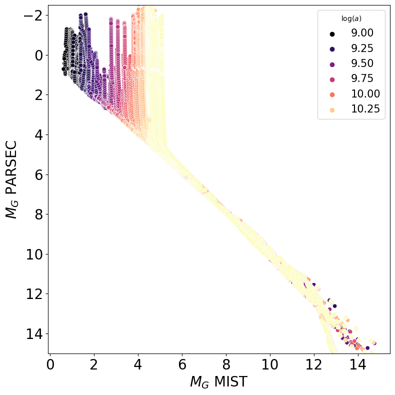
Figure 1: Absolute Gaia $G$ magnitude from PARSEC vs MIST in a region where MIST allocates the combination of parameters as main sequence stars. We do not cut the PARSEC isochrones, to investigate where they differ. We see at brighter absolute magnitudes that PARSEC will evolve stars at a lower mass than MIST will, for a given age and metallicity.

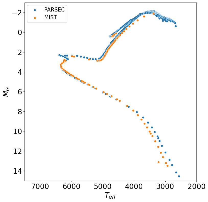
Figure 2: Solar isochrone from MIST and PARSEC. We see that they agree well for main sequence stars. At brighter absolute magnitudes, PARSEC assumes certain masses have evolved to post-main sequence stars while MIST assumes they are still main sequence stars. We will make cuts to focus on regions where the different stellar evolution models agree.

We note that our choice of the Fitzpatrick (1999) extinction curve could be replaced with the Cardelli et al. (1989) (or any other) extinction curve. In comparing these two curves, a difference arises which impacts the computation of the Gaia photometry, with a difference in the extinction coefficient, $A_{G}/A_{0}$, of around 0.04. In our study, this, while worthy of note, does not cause significant issues. Our focus on low extinction regions of the ISM minimises this systematic where we wish to look for relative differences in the extinction. Moreover, in the other passband, this effect is even smaller. Any of the above systematics can be modelled by allowing the error floor on the photometry to absorb these systematic differences.

In Section 4, when generating a synthetic population of stars, a fixed value of $R_{V}=3.1$ is used. However, our model incorporates a more flexible prior on the $R_{V}$ parameter to allow for values normally distributed around 3.1 but we note that this has a small effect on the final posterior. It is important to include this flexibility to account for a real systematic that presents itself in this calculation the posterior of extinction and without this, the posterior is very slightly too narrow. To get an idea of the maximum scale in which $R_{V}$ affects the final extinction we add $A_{0}=1$ extinction to a large grid of stellar parameters and calculate the extinction in each passband using both $R_{V}=4.0$ and $R_{V}=2.5$ and subtract them. In the Gaia bands, we find a mean difference of $0.04$ mag with a standard deviation of $0.013$. In all other bands, the difference is negligible. In the low-extinction regime, the difference in the Gaia bands is very small, but to get the best understanding of the extinction posterior it is necessary to include it.

3.5 Age Assumption

Our model is designed for the analysis of high Galactic latitude stars, which are mainly old. With increasing age, the evolution of sources to a post-main sequence phase happens at lower absolute magnitudes. In Figure 1, we can see in the upper limit our models begin evolving to a post-main sequence phase at around $M_{G}=4$. At magnitudes fainter than this, the age parameter does not change the derived photometry to a large degree. It is important to note, however, that for stars nearer to the solar neighbourhood we might find stars younger than our prior assumption. However, in this region we expect extinction to be very low. Moreover, for the absolute magnitude cuts we will define in the next section, we test our model on finding the extinction distribution for stars younger than our prior and the systematics are negligible.

4 Model Validation on Synthetic Data

In this section, we validate our model on synthetic data sets by using the MIST isochrones (Choi et al., 2016b) to generate synthetic photometry and noisy constraints of the stellar parameters, with the constraint widths akin to current Gaia XP spectra parameter retrieval (in particular Andrae et al. (2023)). We begin by recalling that we are focusing on high Galactic latitudes, where the distribution of stars is dominated by old main sequence stars and our synthetic populations reflect this.

We first probe the stellar parameter space where the stellar evolution models are well-defined. We further validate our model by generating a uniform sample of stars over a large grid of stellar parameters to analyse the degeneracies and the accuracy of retrieving the synthetic extinction value. We inspect how systematic inaccuracies of the stellar models affect the extinction posterior. Moreover, we discuss the implication of prior constraints on the astrophysical parameters, through both functional priors and spectroscopic constraints on the stellar parameters. We also generate a synthetic sample of high Galactic latitude stars using the astrophysical priors outlined in Table 1, with two regions of varying extinction to inspect the success at recovering the spatial variation of extinction.

We find that a spectroscopic constraint on the effective temperature is highly desirable for reducing parameter degeneracies and constraining the extinction posterior distribution, particularly when no prior is assumed on the extinction. However, extinction and the effective temperature are intrinsically related and an assumption on one parameter is an assumption on the other. We derive a method to quantify the degeneracy and illustrate that the posterior mean of both parameters is just one pair of effective temperature-extinction estimates that give a high posterior probability. We derive a relation which can find other extinction-effective temperature pairs which are equally likely under the posterior probability. We stress that the full posterior is needed to summarise these two parameters and reconstruct accurate variation in the ISM, however, we find that by using the posterior mean extinction for each star and smoothing this value spatially, we can detect regions of different extinction if the extinction is spatially correlated. Finding boundaries of interstellar dust is a complicated problem and to attempt accurately detecting small variations in extinction the full extinction posterior needs to be considered.

4.1 Reliable Population of High Galactic Latitude Stars for Constraining Extinction

We analyse the stellar evolution models used in our forward model to find a region of the HR diagram where, for old main sequence stars, the stellar evolution models have a valid solution and can be reliably interpolated over.

We must restrict our stellar models to the region of the HR diagram that is consistent with the allowed parameter ranges from the Castelli & Kurucz (2004) stellar atmosphere models so that we can interpolate over them in [Fe/H] - $\log g$ - $T_{\text{eff}}$ space. We compare this range with the parameters generated by the MIST isochrones for an age range between $10^{8.9}$ and $10^{10.3}$ years. The range of $\log g$ provided by the stellar atmosphere models is from 0.0 to 5.0 dex and the effective temperatures have a lower bound of $3500$ K. To ensure that our interpolation scheme provides a valid solution within the error of the model we restrict ourselves to $3.3<\log g<4.9$ and $3750<T_{\text{eff}}$, where the lower bound on $\log g$ is to mitigate against post-main sequence stars.

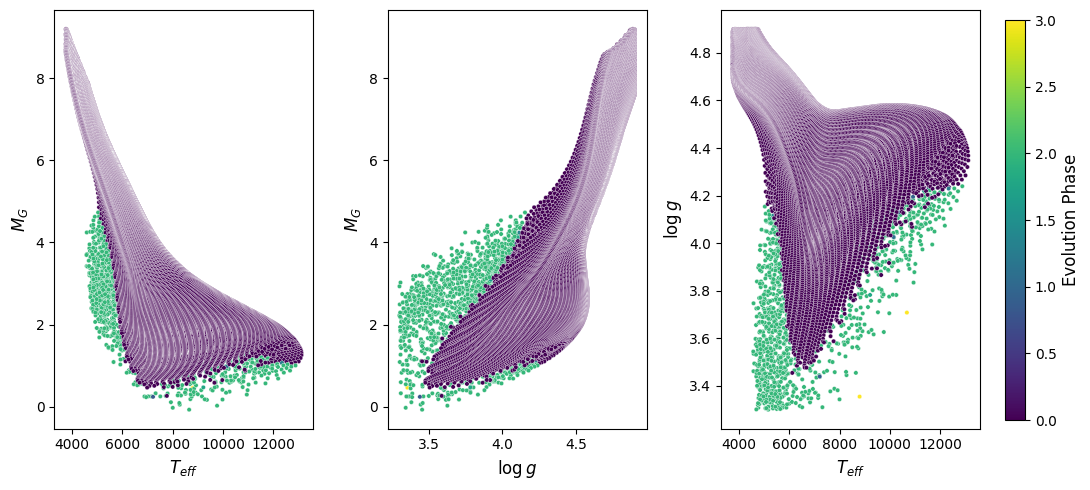
Figure 3: Gaia absolute magnitude $M_{G}$ versus the MIST effective temperature. We illustrate the credible parameter range from stellar atmosphere models, showing where we expect to find post-main sequence stars in the HR diagram. The hue indicates the phase of evolution in the HR Diagram where 0 corresponds to the main sequence.

In Figure 3, we show the result of making the above parameter cuts to the MIST isochrones for a set of isochrones with $8.9\leq\log(a)\leq 10.3$, and illustrate the region of the Gaia HR diagram where valid solutions are feasible. We also make an initial mass cut, $m>0.4$, to reduce the chance of detecting fully convective stars. We wish to restrict the region further to minimise the detection of post-main sequence stars. This amounts to avoiding regions of the HR diagram in Figure 3 where we find sources with a phase greater than $0$. Making such a cut to observed sources will increase the probability of detecting main sequence stars. This has two main benefits; firstly, we are restricted to a region of the HR diagram where stellar evolution theory is most robust and the least systematics are present in choosing a stellar evolution model (see Section 3.4). Secondly, it is in this region of the HR diagram that the majority of the stars in the thick disk (and a significant proportion in the thin disk) at high Galactic latitudes appear. From looking at how the stellar parameter cuts propagate to Gaia absolute $G$ magnitude $(M_{G})$ space, we can define a region of the HR diagram where the stellar models are the most robust for use in our forward model. We see that these cuts correspond to selecting sources with approximately $4.0<M_{G}<8$.

Theoretically, our model can deal with determining the extinction of post-main sequence stars but the accuracy of the stellar models is inconsistent with that of sources along the main sequence, therefore, when applying to real data the contribution of an increased error in theoretical modelling the later stages of a stars life is beyond the scope of this work and not scientifically relevant to our primary focus. Our model would provide an underestimation of the error on $A_{0}$ in this region, which could be a large contaminant when we are looking for small variations in extinction.

If we have a reliable constraint on the surface gravity across the dataset we can make the cut more specific to allow for brighter absolute magnitudes. However, the discussed cut in the Gaia $G$ absolute magnitude should mitigate against finding post-main sequence and fully convective stars. We note that when running the nested sampling procedure, an important flag will be to see if a significant proportion of the posterior mass for the effective temperature and log surface gravity is near the boundaries of the cuts described in this section.

4.2 Uniform Synthetic Sample Generation

To further validate the region in which we can accurately investigate extinction, we generate stars from a large range of stellar parameters and see how our extinction distribution depends on the underlying stellar parameters that generated the star. We begin by outlining the procedure to generate the uniform sample of stars and in further sections discuss the results of running our code on the full parameter range.

We generate a sample of low-extinction stars, with parameters sampled uniformly over a large range. To begin, we model the positional data and its’ measurement error on a high Galactic latitude region by querying a real region of high Galactic latitude with expected low extinction using the Gaia database query. We use the sources in this region to model a realistic distribution of the astrometric and photometric measurement errors as a function of Gaia $G$ magnitude and distance. To generate a single star in the synthetic sample we sample a right-ascension and declination value uniformly from an arbitrary four-degree circle on the high-latitude sky and then sample a metallicity, mass, and $\log(\text{age})$ value uniformly over a $[-2,0.5]\times[0,3]\times[8.9,10.3]$ grid. With a value for the metallicity, mass, and $\log(\text{age})$, we can use our forward model to generate consistent, derived stellar parameters and synthetic photometry $\boldsymbol{\hat{x}}$ in the photometric passbands of interest. Not all initial values of metallicity, mass, and $\log(\text{age})$ generate a solution of the stellar models and we reject all sources with invalid solutions.

Simultaneously, we sample a distance estimate for the region of interest using the prior in Equation 5 and convert it to a parallax value to be included as data. Moreover, we define a realistic parallax measurement error from the distribution of the region as a function of distance. Once we have a value for the metallicity, mass, $\log(\text{age})$, and position we can use the function defined above to generate realistic synthetic measurement error values for estimating each of the stellar parameters. To generate a more realistic sample we add noise to each of the generated features (photometry, metallicity, effective temperature, parallax and other stellar parameters).

For every data point, we simulate the photometry assuming that the model exhibits errors and does not match observation perfectly. We implement this through defining a floor error of $0.05$ mag by setting ${\Sigma}_{jj}=0.05^{2}+\sigma^{2}_{j}$ so that each observed passband magnitude ${\hat{x}}_{j}$ is sampled from $N(x_{j},{{\Sigma}^{2}_{jj}})$, where $\sigma_{j}$ is the synthetic measurement error value from the function modelled on the high latitude region defined above. This is to account for any errors that may arise from the definition of the passbands or incorrect modelling from the isochrones. We chose the value of $0.05$ to account for the maximum difference in the photometry provided by the different sets of isochrones and the difference in the extinction provided by using different extinction laws. Choosing a larger value has the effect of making the posterior distribution wider and allowing for a greater range of extinctions in the posterior samples. If we do not allow for this floor error, the high accuracy of the Gaia photometry dominates the likelihood function and forces the model into a solution which is false due to the systematic error of the theoretical models being greater than the measurement error of the Gaia photometry. In Section 4.4, we inspect the results of assuming the models match observations perfectly within the measurement error.

We add noise to the effective temperature and the metallicity supplied by the theoretical isochrones by assuming it is sampled from a normal distribution, $N(T_{\text{eff}},110^{2})$, and metallicity is sampled from $N([Fe/H],0.1^{2})$. Finally, we use the Fitzpatrick (1999) extinction law with $R_{V}=3.1$ and $A_{0}=0.15$ to add extinction to the magnitudes in each passband. We continually sample until we have $10000$ stars sampled uniformly across the metallicity, mass and $\log(\text{age})$ parameter space. We recall that the widths of the spectroscopic parameter constraints are in line with Andrae et al. (2023), except the effective temperature which has been significantly increased to account for the large degeneracy between effective temperature and extinction.

In our analysis, some of the error values of the sample will be altered to assess the performance of the model. In particular, we will inspect the sample when we have no floor error. Moreover, we will assess the model under uniform priors to illustrate the necessity of astrophysical priors. However, when we do this we mention it explicitly in the following sections.

Data Set	Median $\Delta A_{0}$	Median $\Delta A_{0}$ ($[Fe/H]>-0.3$)	Median Std$(A_{0})$
Uniform prior, $\sigma_{\text{floor}}=0$	$0.075$	$0.168$	$0.113$
Uniform prior, $\sigma_{\text{floor}}=0.05$	$0.206$	$0.461$	$0.209$
$[Fe/H]$ prior, $\sigma_{\text{floor}}=0.05$	$0.058$	$0.291$	$0.159$
$T_{\text{eff}}$ constraint, $\sigma_{\text{floor}}=0.05$	$0.022$	$0.076$	$0.075$
$[Fe/H]$, $A_{0}$ prior, $\sigma_{\text{floor}}=0.05$	-$0.033$	$0.058$	$0.102$

Table 2: Median difference between the posterior mean extinction and the true extinction value of $A_{0}=0.15$, with the median taken over the full synthetic sample. We inspect the accuracy of recovering the extinction when we assume and do not assume a floor error on the photometry. Moreover, see that different constraints on the astrophysical parameters will tighten the extinction posterior around the true value to a differing extent.

4.3 Parameter Sensitivity and Degeneracy: Uniform Priors

Using the generated synthetic samples, we assess the model’s ability to consistently recover input parameters over a uniform grid. In this section, we alter the priors of the model originally defined in Section 3 to be uniform over the grid of parameters generated in the uniform sample. This allows us to explore the likelihood function and illustrate the inherent degeneracies present within. Moreover, we will illustrate the necessity of introducing astrophysical priors or spectroscopic constraints of the stellar parameters. We run the nested sampling algorithm to generate samples of the posterior over the entire parameter space and investigate the sensitivity of the likelihood to each parameter. We test the case where the model exhibits a floor error in the photometry of $0.05$ mag in this section, and the case when the model is perfect (no floor error) in Section 4.4. While we call this section and the subsequent results the ’uniform prior’ section, we still use the IMF as an initial mass prior and use the distance prior defined in Section 3.

We begin by looking at the sample including the floor error on the photometry. We recall that each star in our sample will be a point from the isochrones perturbed by the error from the floor error and the measurement error typical of each passband. We fit our model to each star using the uniform priors on the model parameters. We find that without prior information on the stellar parameters (other than the initial mass), there are significant degeneracies between the model parameters and extinction. Moreover, these degeneracies will cause the width of the posterior to be large.

We recall that each star in the synthetic sample has a true extinction of $A_{0}=0.15$. Under uniform prior assumptions, the model performs poorly in retrieving an accurate point estimate of the model parameters. The median difference between the posterior mean extinction and the true extinction is $0.21$ and the median posterior extinction standard deviation across the sample is $0.209$. The median difference between the posterior mean effective temperature and the true effective temperature is $428.65$ K and the median effective temperature standard deviation across the sample is $346.73$ K. Finally, the median difference between the posterior mean metallicity and the true metallicity is $-0.30$ dex with a standard deviation of $0.52$ dex. In Table 2, we illustrate the extinction posterior median and standard deviations for different cases.

We display the standard deviation, derived from the posterior samples, of the effective temperature, log surface gravity and each of the model parameters in Figure 4. From the posterior samples, we derive the correlation between extinction and the effective temperature, log surface gravity and other model parameters, respectively, which we display in Figure 5. We see that the model is not particularly sensitive to each of the parameters under the assumed errors. In particular, the effective temperature is increasingly hard to constrain at brighter absolute Gaia $G$ magnitudes, $M_{G}$. Moreover, the posterior standard deviation on the extinction parameter is too high to use a point estimate value to constrain the true extinction. This arises because of the significant degeneracies between extinction, the effective temperature, and metallicity, respectively. Therefore, to constrain the extinction further, we need to have a prior constraint on one (or more) of the effective temperature, the metallicity or the extinction parameter itself. Before we inspect the effect of prior constraints on the extinction posterior, we inspect the model when the floor error is zero, thereby assuming the stellar models are perfect in matching stellar parameters to observation.

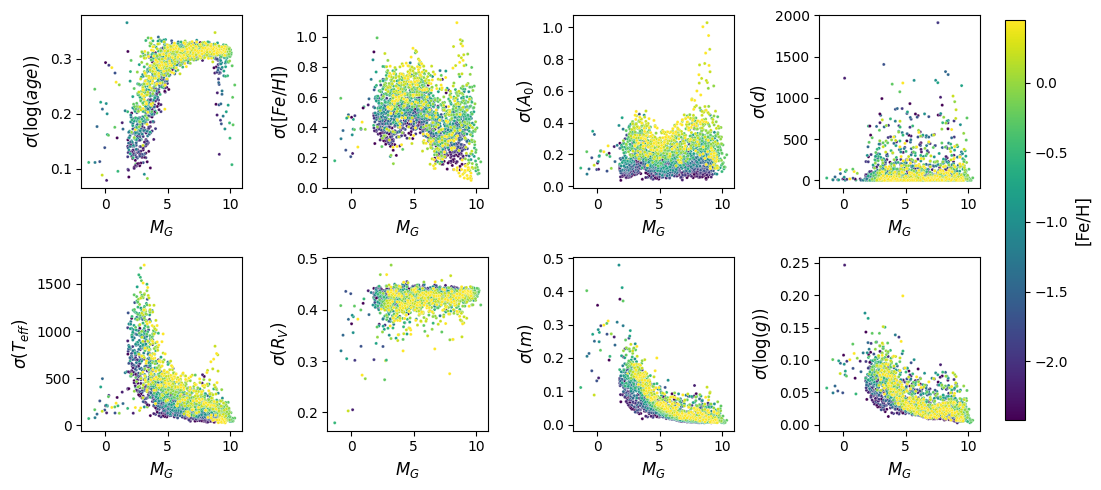
Figure 4: Posterior standard deviation, assuming uniform priors, of the effective temperature, log surface gravity and of each of the model parameters for the uniform sample of stars with an error floor of $0.05$ mag. $M_{G}$ refers to Gaia absolute $G$ magnitudes. We see that when using uniform priors and assuming an error floor, the model is not sensitive to extinction. The true value of extinction in this sample is $A_{0}=0.15$, which is of the same order as the standard deviation of extinction.

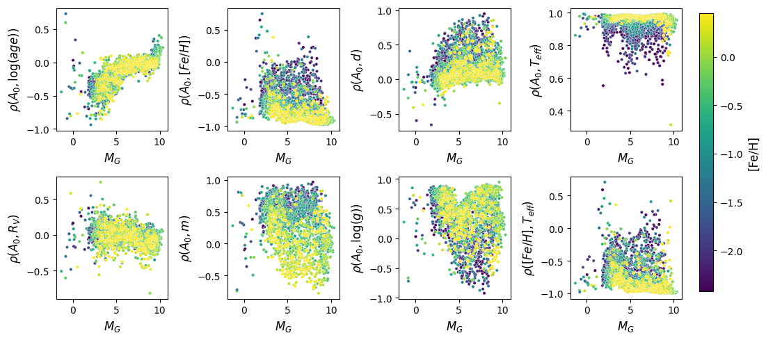
Figure 5: Parameter correlations from posterior samples of each star, assuming uniform priors, for the uniform sample of stars with an error floor of $0.05$ mag. We display the correlation between extinction and the effective temperature, log surface gravity and other model parameters, respectively. $M_{G}$ refers to Gaia absolute $G$ magnitudes. Moreover, in the bottom-right plot, we display the correlation between metallicity and effective temperature. We see that when using uniform priors and assuming an error floor there are significant degeneracies between the extinction, metallicity and the effective temperature. These degeneracies are inherent to the likelihood and some constraint on one of these parameters is necessary to reduce the width of the extinction posterior.

4.4 Floor Error Analysis

There are systematic effects which cause stellar models to mismatch observation for a given input set of stellar parameters. We have identified a region along the main sequence of the HR diagram where stellar models are in the best agreement. In this section, we wish to show how the assumed error floor defined in our model propagates to the final extinction posterior. We recall that the error floor was defined so that the stellar models have a systematic Gaussian error in the output photometry of $0.05$ mag.

To inspect how the floor error affects the final extinction posterior we fit the model once again to the uniform synthetic sample of stars, except now the generated data points have noise only from the synthetic measurement error. In our model construction, we assume the same uniform priors on the model parameters as per the previous section. Moreover, we assume there is no Gaussian noise added to the photometry output of the stellar models.

With no floor error and using uniform priors, we find a median difference between the posterior mean extinction and the true extinction is $0.075$ and the median posterior standard deviation for the extinction parameter across the sample is $0.113$. The median difference between the posterior mean effective temperature and the true effective temperature is $166$ K and the median effective temperature standard deviation across the sample is $284$ K. Finally, the sample median difference between the posterior mean metallicity and the true metallicity is $-0.17$ dex with a standard deviation of $0.43$ dex. In Table 2, we illustrate the extinction posterior median and standard deviations for different cases.

In Figure 6, we show the difference in the posterior standard deviation for each star when the data was generated using a floor error of $0.05$ mag (vertical axes) and when we include no floor error in the synthetic data (horizontal axes). The contours indicate the relative density of points in the diagram. We see that the error floor has a significant effect on the posterior standard deviation of each parameter. In particular, including an error floor in the analysis has widened the extinction posterior by a significant amount. We do not display the correlations of each parameter with extinction as they are unchanged, except for the extinction-effective temperature degeneracy. We find that the effective temperature is globally degenerate with the effective temperature when we have no error floor, this is because, for low metallicity stars along the main sequence, the effective temperature appears to be less degenerate with extinction within the assumed errors of the photometry. When we remove the floor error photometry becomes more sensitive to this degeneracy.

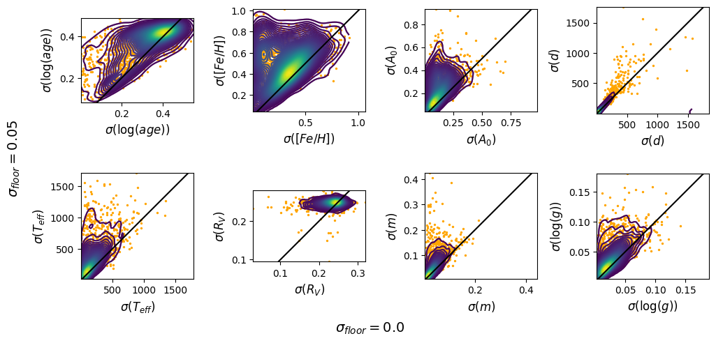
Figure 6: Standard deviation of each parameter derived from the posterior samples when we include a floor error of $0.05$ mag in the synthetic data (vertical axes) and when we include no floor error in the synthetic data (horizontal axes). We overlay the density information on the scatter plot in each case and include the relation $y=x$ as a black line. We see that a floor error will significantly affect the posterior width of the extinction.

4.5 Parameter Sensitivity and Degeneracy: Spectroscopic Effective Temperature Constraint

We have seen that using uniform priors will not sufficiently recover low values of extinction over the uniform sample of synthetic stars we have generated. In this section we show how incorporating a spectroscopic constraint on the effective temperature greatly reduces the width of the extinction posterior. Moreover, we show the extent of the reduction depends on what part of the HR diagram we inspect. We stress that due to the strong degeneracy between extinction and the effective temperature, an assumption on knowing one of these parameters within an error on the constraint is a direct assumption about how well one knows the other. Throughout we assume the photometry includes a floor uncertainty of $0.05$ mag.

We recall that spectroscopic constraints of stellar parameters are included in our model as an estimate of the stellar parameter with an assumed Gaussian uncertainty. Including a constraint on the effective temperature will propagate to both the extinction and the metallicity parameter due to the strong degeneracy between these parameters, so it is of paramount importance not to underestimate the Gaussian error of the stellar parameter estimate.

We run our model on the synthetic uniform sample of stars, assuming that we have a Gaussian constraint on the effective temperature with standard deviation $\sigma_{T}=110$ K. We choose this value as many current stellar parameter studies which derive effective temperatures from the Gaia XP spectra quote mean absolute differences less than this value. Moreover, when we cross-match and compare the Andrae et al. (2023) effective temperatures to the highly accurate Gaia ESO (Gilmore et al., 2022) effective temperatures for a region at high Galactic latitudes we find a mean difference of $110$ K.

We find the accuracy of our model depends on what region of the HR diagram we are investigating. This is due to the effective temperature having a more significant effect on the photometry derived from stellar models as move towards higher-mass stars along the main sequence. Under these assumptions, the model performs well in recovering the true synthetic stellar parameters. We calculate a median difference between the posterior mean extinction and the true extinction of $0.022$ and the median extinction posterior standard deviation across the sample is $0.075$. The median difference between the posterior mean effective temperature and the true effective temperature is $27.35$ K and the median effective temperature standard deviation across the sample is $87.00$ K. Finally, the sample median difference between the posterior mean metallicity and the true metallicity is $-0.003$ dex with a standard deviation of $0.368$ dex. In Table 2, we illustrate the extinction posterior median and standard deviations for different cases.

We display the standard deviation, derived from the posterior samples, of the effective temperature, log surface gravity and each of the model parameters in Figure 7. From the posterior samples, we derive the correlation between extinction and the effective temperature, log surface gravity and other model parameters, respectively, which we display in Figure 8. We see that the model is far more sensitive to each of the parameters under the assumed errors when we have a prior constraint on the effective temperature. We noted before that the effective temperatures were increasingly hard to constrain at brighter absolute Gaia $G$ magnitudes when we had no prior constraint on the effective temperature. Thus, constraining this value will greatly constrain the extinction in the same region of the HR diagram, due to the strong degeneracy between the parameters. We also see that at brighter absolute magnitudes the constraint on the effective temperature will reduce the degeneracy between extinction and the other parameters, in particular, the metallicity.

Due to the degeneracy between extinction and the effective temperature being strong, we find that the ratio between $\Delta(A_{0})/\sigma(A_{0})$ and $\Delta(T_{\text{eff}})/\sigma(T_{\text{eff}})$ is constant for all realistic spectroscopic constraints on the effective temperature ($\sigma_{T}>5K)$. We define $\Delta(A_{0})$ to be the difference between the posterior mean extinction and the true synthetic extinction, moreover, $\sigma(A_{0})$ is the posterior standard deviation for the star. We define $\Delta(T_{\text{eff}})$ similarly. This allows us to demonstrate a rough (but good) approximation of propagating the spectroscopic effective temperature constraint posterior width of the extinction. We display this in the right plot of Figure 9. To derive an approximation of the posterior width when a prior Gaussian constraint with a standard deviation of $\sigma_{T}$ is assumed in the model, we multiply each value along the y-axis of the plot with $\sigma_{T}$ to obtain the width of the extinction posterior as a function of the Gaia $G$ absolute magnitude. It is important to know that this sensitivity is affected by the floor error. This relation will be important if one wishes to constrain the floor error. This roughly tells us the relation between constraining the effective temperature and the extinction.

We stress that due to the strong degeneracy between extinction and the metallicity, an incorrect assumption on the Gaussian bounds of the spectroscopic constraint on the effective temperature will constrain the extinction posterior distribution to an incorrect value. Thus, one must take the utmost care not to underestimate the error on the effective temperature if using such a constraint. We see later on real data how this propagates to the extinction posterior.

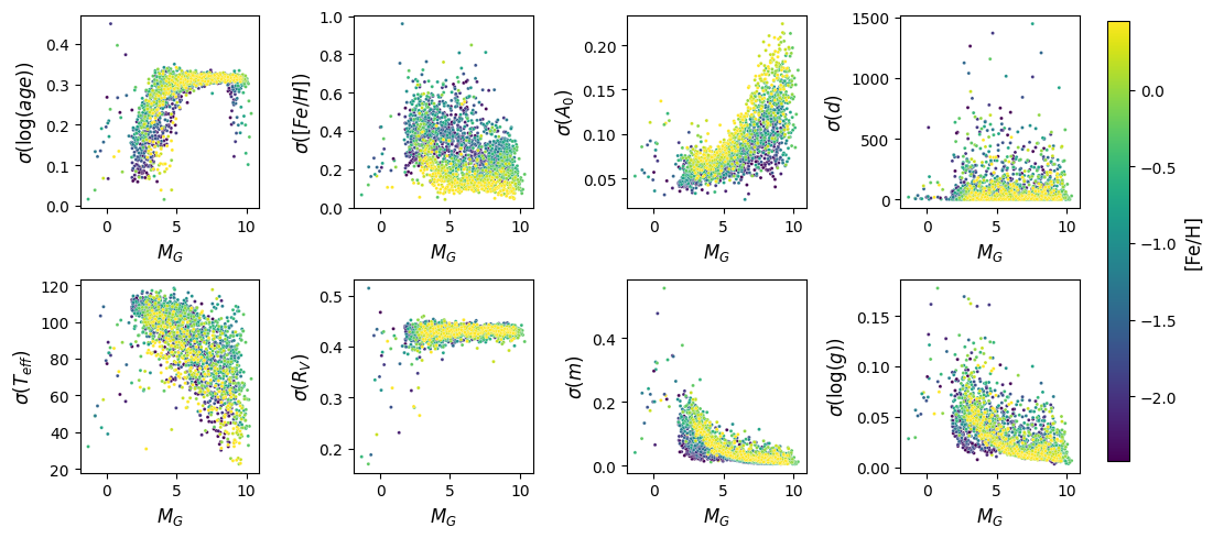
Figure 7: Posterior standard deviations assuming uniform priors, an error floor of $0.05$ mag, and an effective temperature Gaussian constraint with standard deviation $\sigma_{T}=110$ K. We display the standard deviation the effective temperature, log surface gravity and of each of the model parameters for the uniform sample of stars with an error floor of $0.05$ mag. $M_{G}$ refers to Gaia absolute $G$ magnitudes. We see that when using uniform priors, assuming an error floor, and a spectroscopic constraint on the effective temperature, the model is far more sensitive to extinction. The true value of extinction in this sample is $A_{0}=0.15$. We see the posterior extinction standard deviation is reduced for brighter absolute Gaia magnitudes along the main sequence.

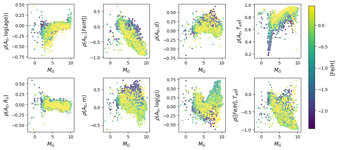
Figure 8: Parameter correlations from posterior samples of each star, assuming uniform priors, an error floor of $0.05$ mag, and an effective temperature Gaussian constraint with standard deviation $\sigma_{T}=110$ K. We display the correlation between extinction and the effective temperature, log surface gravity and other model parameters, respectively. $M_{G}$ refers to Gaia absolute $G$ magnitudes. Moreover, in the bottom-right plot, we display the correlation between metallicity and effective temperature. We see that when using uniform priors, assuming an error floor and having a spectroscopic constraint on the effective temperature significantly affects the degeneracy between model parameters. This will directly reduce the width of the posterior extinction distribution.

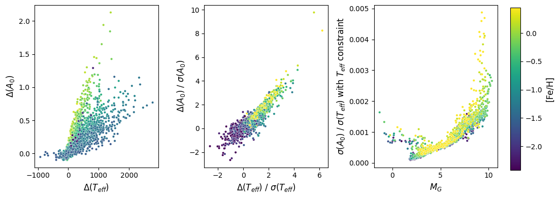
Figure 9: The sensitivity between constraining the extinction parameter and the effective temperature using uniform priors. $\Delta(A_{0})$ and $\Delta(T{\text{eff}})$ represent the difference between the mean extinction/effective temperature and the true extinction/effective temperature, respectively. $\sigma(A_{0})$ and $\sigma(T_{\text{eff}})$ are the posterior standard deviation for the extinction and effective temperature parameter respectively. We find that introducing a spectroscopic constraint on the effective temperature will leave the centre plot invariant. Thus, we can inspect the sensitivity of the effective temperature constraint needed to give a respective constraint on extinction in the right-most plot.

4.6 Parameter Sensitivity and Degeneracy: Astrophysical Metallicity Prior

We now illustrate the results of fitting the model to the data when we incorporate the high Galactic latitude metallicity prior defined in Section 3. Our previous analysis shows that prior constraints on either the effective temperature or the metallicity are necessary to constrain the extinction without adding any prior on the extinction parameter of our model, particularly when we have an error floor on the photometry. We fit our model to the uniform synthetic sample with the error floor of $0.05$ mag included.

We find that the prior on the metallicity significantly improves our ability to constrain the extinction parameter across the whole sample, particularly for stars which have metallicities that are highly likely under our prior assumption. The median difference between the posterior mean extinction and the true extinction is $0.058$ and the median posterior standard deviation is $0.159$. We do not include a tight spectroscopic constraint on the metallicity as a Gaussian term in the likelihood function using a value from spectroscopic surveys due to it being difficult to calibrate spectroscopic metallicities to those from stellar evolution code. We do not wish to introduce any unknown systematic error when training to constrain values of extinction, thus, we incorporate our spectroscopic knowledge of the metallicity via an astrophysical prior.

We display the posterior standard deviation of the effective temperature, log surface gravity and each of the model parameters in Figure 10. We see that the model is far more sensitive to to each of the parameters under the assumed errors when we have a high Galactic prior on the metallicity. In particular, the metallicity, extinction, and effective temperature posterior standard deviations are reduced over the sample. We omit an illustration of the correlations due to them being relatively invariant from Figure 5.

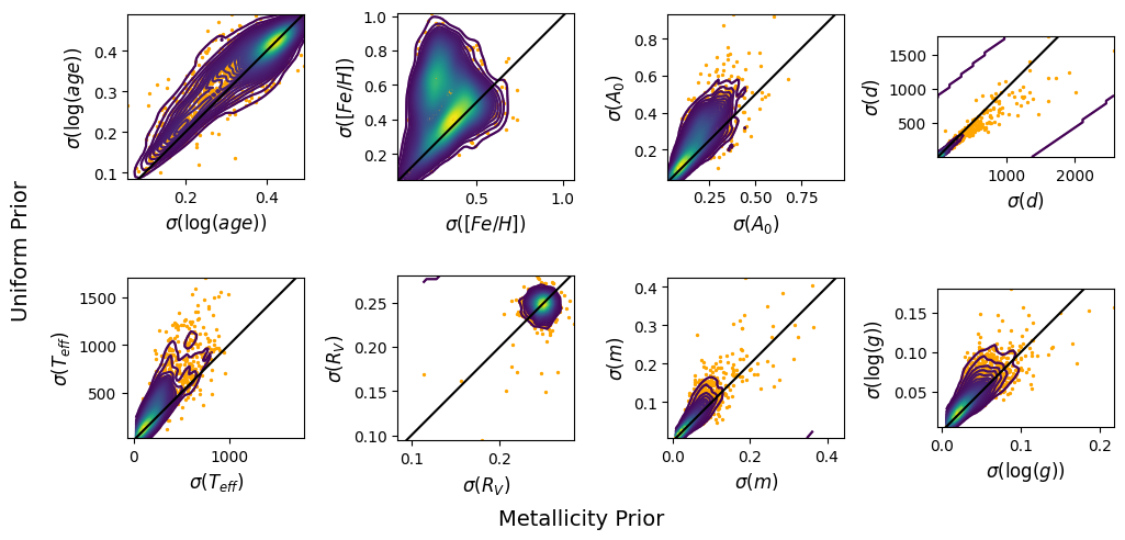
Figure 10: Parameter standard deviations from posterior samples of each star with an error floor of $0.05$ mag on the photometry when (vertical axes) assuming a uniform prior on the metallicity versus (horizontal axes) using a metallicity prior derived from LAMOST metallicities at high Galactic latitudes. We see that the metallicity prior is useful in constraining the extinction, metallicity and effective temperature.

Due to the degeneracies between metallicity and other parameters, our model is not particularly sensitive to metallicity using just these photometric passbands (see Appendix A). Sources with true metallicity with a low prior probability will return a false metallicity point estimate and bias the effective temperature and extinction point estimates to an inaccurate value. We can see this effect by comparing the difference between our posterior mean extinction and the true extinction for each star against the difference between the posterior mean effective temperature and the true effective temperature. We display a plot of this comparison in Figure 11, where outside the metallicity prior we have increasingly bad point estimates for extinction.

More flux observations in the optical wavelength range allow one to constrain the metallicity better for such stars. Constraining the metallicity reliably can be contaminated by systematics from the stellar models. In future work, we will look at accurately calibrating the Gaia BP/RP spectra to be used as spectral observations in our model. This will allow us to further constrain the metallicity and provide more robust extinction estimates, particularly for outlier sources which lie outside our metallicity prior.

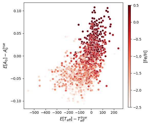
Figure 11: Comparing the difference between our posterior mean extinction and the true extinction for each star against the difference between the posterior mean effective temperature and the true effective temperature, for the uniform sample using a metallicity prior. The relative occurrence of points in this diagram is not relevant as the samples have been generated to be uniform over the metallicity prior bounds.

4.7 Low Extinction Prior

We have seen that extinction is highly degenerate with both the effective temperature and the metallicity, and how prior constraints on each of these parameters propagate to the extinction posterior distribution. If prior knowledge about the extinction distribution is known, we can incorporate a relevant prior into our model. At high Galactic latitudes, we expect the extinction to be low, and a natural probability distribution to choose as a prior on the extinction parameter is an exponential distribution. This is a typical choice used to represent prior knowledge about low extinction sightlines and is common in Type Ia supernovae modelling (see, for example, Mandel et al. (2022)).

We stress that due to the significant degeneracy between extinction and the effective temperature, a prior distribution on the extinction parameter acts as a prior distribution on the effective temperature and needs to be considered carefully when used in conjunction with a spectroscopic constraint on the effective temperature. Moreover, for an exponentially distributed random variable, $X$, with rate parameter $\lambda$, the width of the distribution is given by $\sigma(X):=\sqrt{\text{Var}(X)}=1/\lambda$. Thus, if the extinction parameter is sampled from an exponential distribution, $A_{0}\sim\text{Exp}(\lambda)$, due to the strong correlation between extinction and effective temperature the prior will propagate to the effective temperature and restrict the posterior to a region approximately given by $\sigma(T_{\text{eff}})\approx\frac{1}{\alpha\lambda}$, where $\alpha$ corresponds to the value of $\sigma(A_{0})/\sigma(T_{\text{eff}})$ from the right plot of Figure 9. Thus, we see that such a prior on extinction is a strong assumption about extinction and the effective temperature.

We fit our model to the uniform synthetic sample with the error floor of $0.05$ mag, assuming the astrophysical prior on the metallicity, an exponential prior (with $\lambda=1.5,5)$. Moreover, we do not include a spectroscopic constraint on the effective temperature. We find that the prior on the extinction significantly improves our ability to constrain the extinction parameter because we knew that the extinction in this sample was low. Using a value of $\lambda=1.5$ only slightly tightens the extinction posterior distribution from the case when using the astrophysical metallicity prior. However, when using the extinction prior with $\lambda=5$, we see further improvements. The median difference between the posterior mean extinction and the true extinction is $-0.033$ and the median posterior standard deviation is $0.114$ over the sample. Moreover, the median difference between the mean posterior effective temperature and the true effective temperatures over the full sample is $-33.49$ K and the median standard deviation on the posterior effective temperatures is $152$ K. Finally, the median difference between the mean posterior metallicity and the true metallicities over the full sample is $0.1$ dex and the median standard deviation on the posterior metallicity is $0.25$ dex. Thus a reliable extinction posterior can prove to be invaluable when constraining true values. It is useful to use emission maps, such as the Planck dust map (Planck Collaboration et al., 2016), to get regional estimates of the upper limit of $A_{0}$.

4.8 A Family of Equally Likely Extinction-Effective Temperature Pairs

The strong degeneracy between extinction and effective temperature allows for a large family of point estimates which give a similar posterior probability under the assumed model errors. Introducing priors and spectroscopic constraints only restricts our posterior to a subset of this family. We illustrate the posterior samples of effective temperature and extinction which achieve close to maximum posterior probability for a single star in the left image of Figure 12, assuming uniform priors and a floor error of $0.05$ mag.

We find that the ratio $\sigma(A_{0})/\sigma(T_{\text{eff}})$ can be described as a function of the effective temperature and it is invariant of the prior distributions on the stellar parameters. The introduction of priors (provided they are not extremely narrow) does not remove the degeneracy but restricts the degeneracy to a subset of the parameters. We display this relation in the right plot of Figure 12, and note the ranges of effective temperatures in both images. Unconstrained by priors, the range of effective temperatures and extinctions is approximately given by the length of the intersection between the line passing through the parallax-corrected photometric point in the direction of the extinction vector, and isochrone manifold in photometric space. This intersection depends on the errors of the model and higher errors mean more points on the manifold will appear to intercept the line.

We can successfully use this relation to ’transform’ extinction into effective temperature and vice versa. If we have an effective temperature and extinction pair, $(T_{\text{eff}},A_{0})$, we can convert a small amount of extinction, $\delta A_{0}$, into a small change of effective temperature via the relation $\delta T_{\text{eff}}=-\delta A_{0}(\sigma(A_{0})/\sigma(T_{\text{eff}}))$, by using $\sigma(A_{0})/\sigma(T_{\text{eff}})$ to move along the curve in the right plot of Figure 12. Moreover, we can perform this operation repeatedly to move along the degeneracy and generate a family of pairs with similar posterior probability, provided we do not move suitably far away from the posterior mode. This is particularly useful when comparing results against spectroscopic surveys. The non-linearity of the curve can be reduced if we further constrain the metallicity.

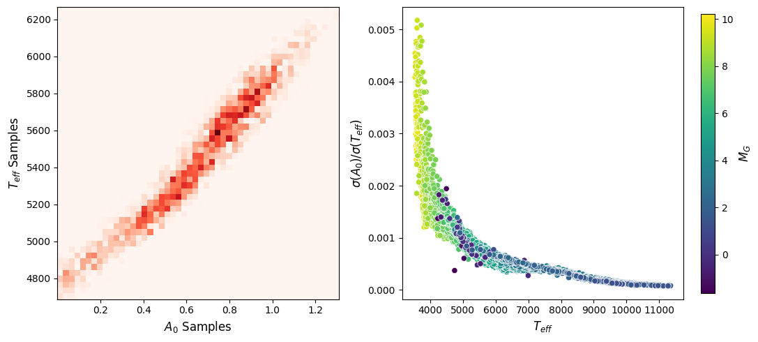
Figure 12: Left plot: Posterior samples of the effective temperature and extinction parameters for a single, synthetic star assuming uniform priors and a floor error of $0.05$ mag. Right plot: the ratio, $\sigma(A_{0})/\sigma(T_{\text{eff}})$, for different values of $T_{\text{eff}}$. The hue indicates the absolute Gaia $G$ magnitude of the point. We note that this ratio is invariant of prior assumptions on the metallicity, effective temperature and extinction unless they are particularly narrow. In particular, constraining the metallicity will reduce the non-linearity of the curve.

4.9 Resolving Regions of Different Extinction

We introduce a typical sample generated using the astrophysical priors with varying extinction to show that in low-extinction regions we can use the posterior extinction mean and standard deviation to construct dust maps. Many other dust maps bin the sources into sightlines (such as Green et al. (2019)) or introduce a prior on the spatial distribution of the extinction parameter. This paper is an illustration of the intricate details in deriving the posterior distribution for a high Galactic latitude star, therefore, we assume that the posterior distribution of a single star is the full information for a single source and any smoothing or analysis on a spatial basis is carried out based on these distributions, not by forcing the correlation to appear in the posterior. When generating dust maps, this has the downside of not utilising the knowledge that extinction should be non-decreasing along a line-of-sight. We carry out this brief analysis to illustrate the complications which may arise. Moreover, even if we assume there is spatial or radial correlation, when we look to constrain the extinction for each sightline we will still be fitting our model to detect small variations in extinction and the intricate details of the posterior are still relevant. Moreover, in this section, we assume the floor error is $0.05$ mag and that our model priors are as per Section 3 unless specified otherwise.

We generate a new synthetic sample similar to Section 4.2, except now using the priors outlined in Table 1 and selecting two specific regions of different extinction. Once again, we query a real region of high Galactic latitude with expected low extinction using the Gaia database query to find a realistic distribution of the astrometric and photometric measurement errors as a function of Gaia $G$ magnitude and distance. We sample a metallicity, mass and $\log(\text{age})$ value from their respective prior distributions and pass these values to our forward model to generate consistent stellar parameters and synthetic photometry in the photometric passbands. We sample a distance estimate for the region of interest using the prior in Equation 5 and convert it to a parallax measurement. With these generated stellar features we transform the values to noisy apparent magnitudes, parallaxes and $[Fe/H]$ and $T_{\text{eff}}$ values by adding Gaussian noise to the photometry (with a floor error of $0.05$ mag) and parallax consistent with the queried Gaia sample and Gaussian noise of $0.1$ dex and $110$K to the $[Fe/H]$ and $T_{\text{eff}}$, respectively.

Finally, we use the Fitzpatrick (1999) extinction law with $R_{V}=3.1$ to generate two different samples with different regions of extinction. We create a uniform, dimensionless square grid between $-1$ and $1$ by randomly allocating the synthetic stars across the grid. In the first case, we generate a ring region with width $0.1$ in the $x-y$ plane. The ring will have a constant true $A_{0}$ value of $0.2$, which increases every $500$ pc radially by $0.02$m with a ceiling of $0.26$. Everywhere else in the grid will have a fixed value of $A_{0}=0.1$. The second region will be defined similarly, except we generate a circular region instead of a ring. We display plots of the regions in the left column of Figure 13, where the top row shows the plots when the increased extinction region forms a ring and the bottom row shows the plots when it forms a circle. The extinction values have had a Gaussian smoothing filter applied to them over the spatial dimensions, which explains the gradient in the ground truth plots (left-most column).

We fit the model to the data in three cases. Firstly, when we run our model with no spectroscopic constraints. Secondly, when we assume a spectroscopic effective temperature constraint with a Gaussian error of $\sigma_{T}=110$ K, and finally, when we include a prior assumption that $A_{0}$ is distributed like $A_{0}\sim\text{Exp}(\lambda=5)$. We find that the model can somewhat reproduce both extinction regions in the cases when we assume either a spectroscopic constraint on the effective temperature or the prior distribution on the $A_{0}$ parameter. However, when we make no prior assumptions on the extinction or effective temperature we can only roughly reconstruct the circular region, and cannot reconstruct the ring region.

We illustrate these results in Figure 13, where we display the ratio $\text{E}[A_{0}]/\sqrt{\text{Var}[A_{0}]}$ (where the expectation and variance are calculated for each star using the respective posterior) after applying a Gaussian filter to smooth the values spatially. The middle column displays the case when we do not use any spectroscopic constraint of the effective temperature or extinction prior. We can see when the high extinction region is a ring, there is too much noise to recover any significant signal and we cannot reconstruct the true topology of the synthetic cloud. However, when the region is a circle, we can somewhat reconstruct the high extinction region, although we note that there is significant noise which could be interpreted as artificial structure. In the final column, we show the case when we include a spectroscopic constraint of the effective temperature with Gaussian width $\sigma_{T}=110$ K. We can see in the ring case that there is a significant correlation with the true extinction values. However, we note that there is also a lot of noise which could be falsely interpreted as real structure. In the circular case, we can almost perfectly reproduce the region. The noise arises from the posterior standard deviation of extinction being large compared to the posterior mean extinction. Future work will look to use the full posterior to quantify the noise in these dust maps and work towards confidently detecting small variations in the ISM.

We note that the dust maps generated using the exponential extinction prior will be almost identical to those generated by using the spectroscopic constraint of the effective temperature when we make a suitable Gaia absolute $G$ magnitude cut. This is no coincidence, and we chose the value of $\lambda=5$ to reflect this. We recall from Section 4.7, that we can approximate the width of the effective temperature posterior via dividing $1/\lambda$ by the value on the $y$ axis of the right plot in Figure 12. We chose a value of $\lambda=5$ to give us a mean value of approximately $\sigma(T_{\text{eff}})\approx 110$ K within our absolute magnitude cut.

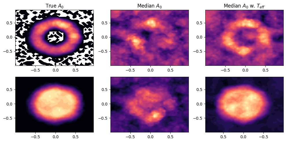
Figure 13: The ratio $\text{E}[A_{0}]/\sqrt{\text{Var}[A_{0}]}$ (where the expectation and variance are calculated for each star using the respective posterior) derived from the synthetic regions with varying extinction. The left column illustrates the ground truth, the middle shows the map when using only a metallicity prior. The right column shows the results using an effective temperature estimate (or, equivalently, an extinction prior). For the top row the model is a ring, for the lower row the model is a circle.

5 Model Validation With Real Data

We further validate aspects of our model using real photometric, parallax and spectroscopic data. We illustrate how sensitive the extinction posterior is to assuming a prior knowledge of the extinction parameter or a spectroscopic estimate of the effective temperature.

We fit our model to a sample cross-matched with the LAMOST DR8 (Wang, 2022) spectroscopic parameters and show that misconceptions may arise when considering point estimates of effective temperature and extinction. In particular, a statement about the effective temperature is a statement about the extinction and, even though we generate posterior mean effective temperatures systematically different to LAMOST’s, we can use the extinction-temperature degeneracy to accurately reproduce LAMOST’s effective temperatures. Thus, we stress the use of a full extinction posterior as the full information.

We use stellar parameters derived from Gaia ESO (GES) iDR6 (Randich et al., 2022) to show that if one has an independent and accurate method of constraining the effective temperature in a region we can calibrate the extinction prior so that our zero point on extinction matches the expected value from the region. In the same sample, we show that we can detect outliers by comparing the extinction posterior to a well-calibrated extinction prior.

We compare data from different surveys to illustrate that accurate bounds on a spectroscopic constraint of the effective temperature are essential to avoid forcing a false extinction posterior. Finally, we run our algorithm on a region studied by Panopoulou et al. (2019), and generate a dust map using spatial Gaussian smoothing to compare with other dust maps.

5.1 Comparison with LAMOST Derived Parameters

In this section, we validate our model against the LAMOST DR8 (Wang, 2022) spectroscopic parameters which have been derived using the LASP stellar parameter model (Wu et al., 2014). We note that for high Galactic stars, both LASP and the LAMOST Spectrograph Response Curves (Du et al., 2016) ignore the effects of interstellar extinction when deriving stellar parameters. We will show that our mean posterior effective temperatures match the LAMOST effective temperatures when we convert our mean extinction into an effective temperature term through the transformation along the extinction-effective temperature degeneracy, introduced in Section 4.8.

We select sources from LAMOST with Galactic latitude $|b|>60^{\circ}$ and cross-match with Gaia DR3, 2MASS and ALLWISE as outlined in Section 2. Moreover, we cross-match our sources with the APOGEE DR16 (Jönsson et al., 2020) stellar parameters. However, in this section, we assume that the lower resolution LAMOST stellar parameters are the ground truth and illustrate the differences which arise in Appendix C. We remove all sources with LAMOST effective temperature error greater than $50$ K to match the mean error in effective temperature quoted by Andrae et al. (2023). For the same reason, we remove all sources which exhibit a metallicity error greater than $0.1$ dex. Finally, we remove all sources with distance from Bailer-Jones et al. (2021) exceeding $2$ kpc to mitigate against the effects of parallax error.

We fit our model to the photometry and parallax data assuming a prior extinction distribution of $A_{0}\sim\text{exp}(\lambda=5)$. Recall that this distribution has a mode of $A_{0}=0$, a mean of $A_{0}=0.2$ and standard deviation $\sigma(A_{0})=0.2$. This is a reasonable prior at these latitudes but is not too tight to fix the extinction to very low values. We will see that, because we understand the extinction-effective temperature degeneracy very well (see the right plot in Figure 12), we can convert extinction to effective temperature and vice versa, allowing us to inspect the posterior assuming a strong zero extinction prior.

We discuss the difference between the posterior mean effective temperature, metallicity and log surface gravity values with the LAMOST values for each star. We find that there is a systematic offset between our mean effective temperatures and those derived by LAMOST with a median difference in the sample of $223.12$ K. The median standard deviation of the effective temperature across the sample is $173.90$ K. The median difference between the posterior metallicity and the LAMOST-derived metallicity is $-0.02$ dex, and the median standard deviation of the posterior metallicity across the sample is $0.20$ dex. The median difference between the log surface gravity derived from the posterior and LAMOST’s values is $0.05$ dex, and the median posterior standard deviation across the sample is $0.04$ dex.

These systematic differences can be misleading due to the strong degeneracy between extinction and the effective temperature of a star. We recall that the two parameters are intimately related via the curve in the right plot of Figure 12. In our model, we have allowed for stars to have non-zero extinction so that there is a reasonable prior probability of stars having an extinction value of $A_{0}=0.2$. This assumption means that the effective temperature and extinction degeneracy have not been fixed but restricted to a region dictated by the prior on $A_{0}$. Therefore, the point estimate of the effective temperature does not represent the value you would obtain if you assumed zero extinction, but has been restricted to a range dictated by the extinction prior and the data. However, LAMOST fixes the extinction to zero in their derivation of the effective temperature.

Therefore, when taking mean values of the posterior we expect our effective temperatures to be systematically different. Through the relation in Figure 12, we can transform extinction values into effective temperature along the vector of degeneracy. Here, we wish to transform all of the extinction for each star into effective temperature, thus, we transform our posterior mean effective temperature as $E[T_{\text{eff}}]\mapsto E[T_{\text{eff}}]-E[A_{0}]\frac{\sigma(T_{\text{eff}})}{\sigma(A_{0})}$, or like $E[T_{\text{eff}}]\mapsto E[T_{\text{eff}}]-E[A_{0}]E[\frac{\sigma(T_{\text{eff}})}{\sigma(A_{0})}]$ as an approximation if we wish to use a constant value of $\sigma(T_{\text{eff}})/\sigma(A_{0})$ (see Section 4.8 for a background to this transformation). Each of the expectations is taken over the posterior for each star. We display a plot of LAMOST’s derived effective temperatures together with our derived posterior mean effective temperatures, and the corrected temperatures, respectively, in Figure 14.

In the left-most plot of Figure 14 we see the LAMOST effective temperature values against the posterior mean effective temperatures for each star in the sample. There is a clear systematic between the two sets of effective temperatures, but we note that it is not uniform across all temperatures. In the middle and right-most plot, we see where this systematic arises from. By converting the posterior mean extinction for each star into effective temperature we can recover the effective temperatures derived by assuming no extinction. The middle plot shows the correction by applying the uniform transformation $E[T_{\text{eff}}]\mapsto E[T_{\text{eff}}]-E[A_{0}]E[\frac{\sigma(T_{\text{eff}})}{\sigma(A_{0})}]$ and we see a strong correlation between the two sets of effective temperatures. In the right-most plot, we transform by assuming the value of $\frac{\sigma(T_{\text{eff}})}{\sigma(A_{0})}$ from Figure 12, where we also see a strong correlation.

The correct transformation to make is the one which accounts for what part of the HR diagram one is probing (right plot). We can see that this transformation will accurately reconstruct the LAMOST effective temperatures. However, it introduces a slight curve around the line $y=x$. We stress that by introducing an extinction prior, one expects these systematic differences in posterior mean effective temperatures as the width of the posterior depends on which part of the HR diagram one probes. The effective temperature and the extinction parameter are intimately related and one can only compare effective temperatures reliably as point estimates when a good understanding of the extinction prior is known and accounted for. This systematic bending effect, while slight here, has been seen before (see Hegedűs et al. (2023)) in a more pronounced fashion, particularly when comparing the effective temperatures derived from the APOGEE survey with others. We will illustrate in Appendix C that one can derive higher correlations between LAMOST and APOGEE using this correction. However, it is important to note that these corrections are mathematical and all we do is choose a set of parameters which achieve similar posterior probability. Unless an extra independent constraint on the effective temperature is known, the full solution is the extinction posterior.

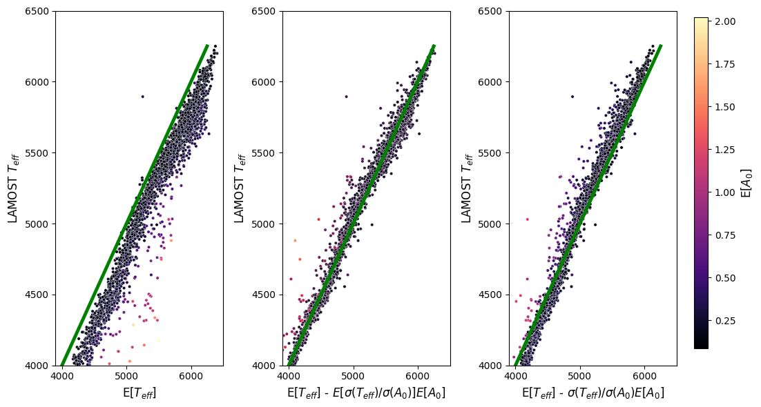
Figure 14: Comparison of posterior mean effective temperatures with LAMOST illustrating that we can reproduce the LAMOST effective temperatures. In the left-most plot, we see the LAMOST effective temperature values against the posterior mean effective temperatures for each star in the sample. By converting the posterior mean extinction for each star into effective temperature we can recover the effective temperatures derived by assuming no extinction. The middle plot shows the correction by applying the uniform transformation and in the right-most plot we make the transformation using the relation from Figure 12.

We see in Figure 14, that there are points which remain as outliers and our model has identified them as points with high extinction. It is highly unlikely that all of these outliers have such high extinction. We find from the synthetic analysis that, at low effective temperatures, this excess in extinction can arise from observing a binary system or star considerably younger than our prior allows for. To understand and flag these points, it is useful to have a well-calibrated extinction prior for the region. To do this, we use Gaia ESO to provide effective temperatures which have been derived using an extinction-independent method.

5.2 Towards Finding Extinction Zero-Points Using Gaia ESO

In the previous section, we showed that we could reliably reproduce the LAMOST effective temperature values if we assumed that there was no extinction in the sample. This was because the LAMOST effective temperatures were derived by assuming there is no extinction for high Galactic latitude stars when deriving stellar parameter estimates.

In this section, we wish to use stellar parameters which have been derived without assuming zero extinction and using methods independent of ours. We use the highly accurate spectroscopic features from Gaia ESO (GES) iDR6 (Randich et al., 2022) and show how well we can reconstruct the same stellar parameters.

We query the GES survey for sources at high Galactic latitude ($|b|>45^{\circ}$) which have a valid $[Fe/H]$ and $T_{\text{eff}}$ value with a measurement error of less than $0.1$ dex and $110$K for the metallicity and effective temperature, respectively. The GES values for the error on the stellar parameters estimates are robust, due to the survey being rigorous in deriving the values using multiple methodologies (Gilmore et al., 2022). GES iDR6 has been pre-matched with the Gaia DR3 database, allowing us to query each of our selected targets from the database and retrieve a complete Gaia solution. Furthermore, we cross-match the Gaia sources with 2MASS and ALLWISE as outlined in Section 2 and make all quality cuts as described therein. Finally, we remove all sources with $\log g<4.0$, and make an absolute magnitude cut (using the parallax) of $7.5>M_{G}>4.5$, leaving us with a final sample size of 990 sources.

We fit our model to the data using an exponential prior on $A_{0}$ with $\lambda=5$. We discuss the difference between the posterior mean effective temperature, metallicity, and log surface gravity values for each star in comparison with the GES values. We find that there is a systematic offset between our mean effective temperatures and those derived by GES with a median difference in the sample of $136.04$ K. The median standard deviation of the effective temperature across the sample is $183.0$ K. The median difference between the posterior metallicity and the GES-derived metallicity is $0.276$ dex, and the median standard deviation of the posterior metallicity across the sample is $0.21$ dex. The median difference between the log surface gravity derived from the posterior and GES’s value is $0.05$ dex, and the median posterior standard deviation across the sample is $0.04$ dex.

Recall that, via the transformation described in Section 4.8, we can transform extinction into effective temperature and leave the point invariant in the observed data space within the errors of the model. We can use this relation to find a zero point of extinction in our sample assuming that the effective temperatures from GES are complete in accounting for the effective temperatures in an extinction-independent manner.

To illustrate this we show three different cases for our transformed effective temperature in Figure 15. From the left, the image shows the effective temperatures derived from GES versus the unaltered posterior mean extinction for each point in the sample. The middle plot shows the GES effective temperature versus the mean posterior effective temperature after subtracting all of the posterior mean extinction. To generate the final plot, we generate values of $\delta A_{0}$ and transform them to the effective temperature by subtracting this contribution. We chose the value which gave the best fit between the transformed effective temperature and the GES effective temperatures. This amounts to taking an $\delta A_{0}=0.1$ amount of extinction, transforming it and subtracting it from the posterior mean effective temperature.

We can analyse the amount of extinction which remains after this transformation. We find a median value of $A_{0}=0.12$ for this transformed sample. We query the Planck (Planck Collaboration et al., 2016) dust map for the Galactic coordinates of each of the stars in this sample and find a mean value of $A_{V}=0.13$. Thus, having highly accurate, independent constraints of effective temperature will be useful in calibrating the extinction zero-point of a region. We can calibrate the exponential extinction prior by setting $\lambda=8.5$, so that we expect sources to have low extinction, but the prior mean extinction is approximately $A_{0}\approx 0.12$. If we fit our model with this revised prior we will have effective temperatures calibrated to GES’s values.

We note, however, that without an extinction-independent method to derive accurate effective temperatures, a full posterior over these parameters is necessary to constrain a variation in extinction. Moreover, if using point estimates of the effective temperature and extinction one needs to be particularly careful what prior information has been included to derive those values. Extinction values, as point estimates, derived from GES are incompatible with point estimates of the effective temperatures from LAMOST as they assume different assumptions about extinction. Moreover, calibration does not change our posterior uncertainty on the parameters. We recommend calibrating to effective temperatures in this manner, as opposed to directly using the effective temperature as a spectroscopic constraint. We will see that if we wish to use a spectroscopic constraint directly, it is highly dependent on the bounds of the constraint.

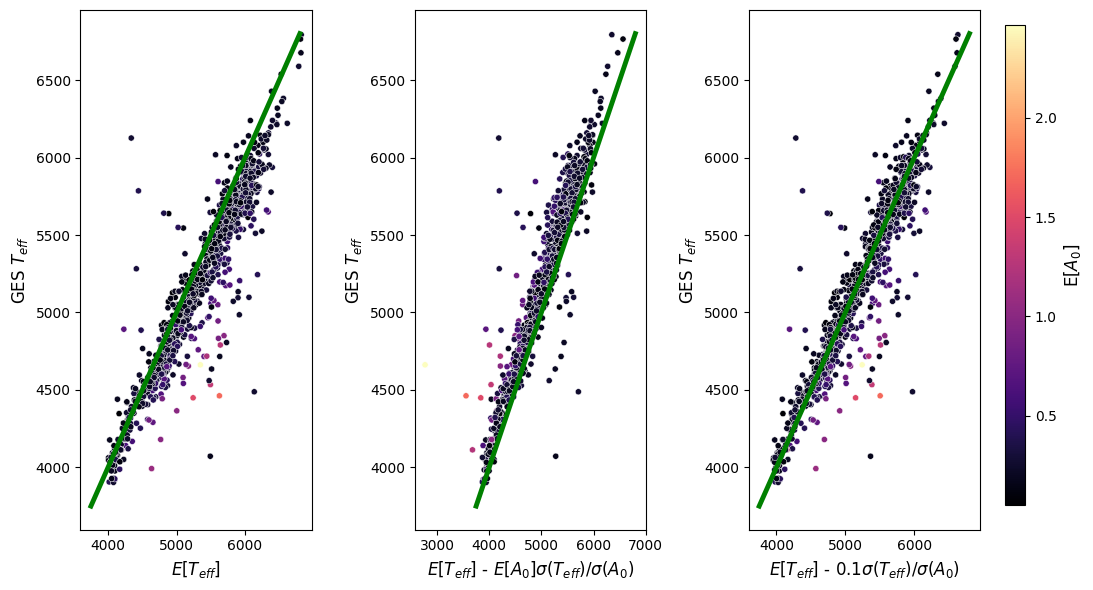
Figure 15: Calibrating the extinction prior to the effective temperatures derived by Gaia ESO. From the left, the image shows the effective temperatures derived from GES versus the unaltered posterior mean effective temperature for each point in the sample. The middle plot shows the GES effective temperature versus the mean posterior effective temperature after subtracting all of the posterior mean extinction. The right plot shows the transformation using the zero-point extinction value which gave the best fit between the transformed effective temperature and the GES effective temperatures. This amounts to subtracting a $\delta A_{0}=0.1$ amount of extinction from the posterior mean effective temperature.

5.3 Outliers from GES Sample

We use the same sample as the previous section, derived by cross-matching high Galactic latitude sources from Gaia ESO with Gaia, 2MASS and ALLWISE, to show that high extinction points may be outliers and further analysis should be carried out. We display a plot of the distance corrected Gaia HR diagram for the region in Figure 16. The plot shows a narrow main sequence with a small scatter and a few points with a significant scatter on the right of the main sequence. These points have been characterised as stars with relatively high extinction. We suspect that some of these stars may be binary stars, others young stars and some genuinely high extinction points.

We stress this because some algorithms choose to smooth spatially over extinction values in the inference step. This would mitigate against outliers, but would also suppress small regions of genuinely high extinction if they existed in the sample. Thus, flagging stars with improbable extinctions under a well-chosen prior is necessary for outlier detection. We suspect, from synthetic analysis, that these outliers are either binary systems or young stars.

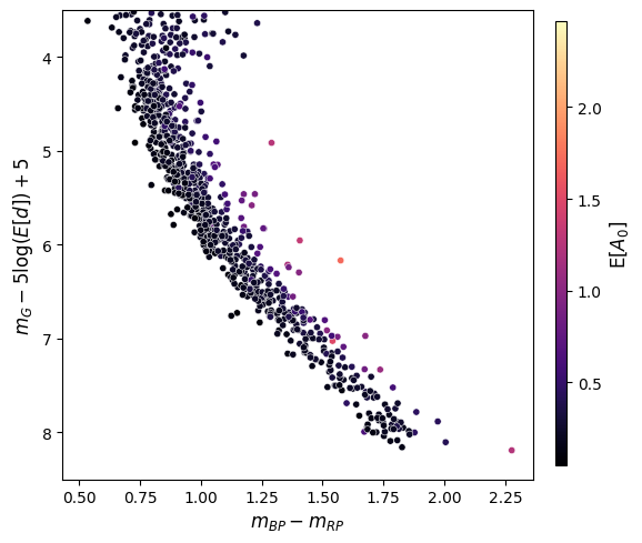
Figure 16: The distance corrected Gaia HR diagram for the region using the Gaia ESO cross-matching. The plot shows a narrow main sequence with a small scatter and a few points, potentially outliers, lying relatively far away from the main sequence.

5.4 Sensitivity to the Width of the Spectroscopic Constraint

In this section, we illustrate the caution that needs to be accounted for when using spectroscopic-derived stellar parameter estimates to constrain extinction. It is well-known that extinction is degenerate with effective temperature, but it is important to note that the degeneracy is not uniformly strong across all of the parameter space (as seen in Section 4.8).

We describe a method of validating our model using highly accurate spectroscopic features from Gaia ESO (GES) iDR6 (Randich et al., 2022) and show how well we can reconstruct the same extinction distribution by using the Andrae et al. (2023) astrophysical parameters estimates (AAP). It is noteworthy that the AAP values were derived using similar data to our method, therefore, we cannot perform real inference using these parameters. However, using their values, we will restrict our extinction posterior so that our effective temperature is centred on their value for illustrative purposes.

We query the GES survey for 2000 sources at high Galactic latitude ($|b|>30^{\circ}$) which have a valid $[Fe/H]$ and $T_{\text{eff}}$ value with a measurement uncertainty of less than $0.1$ dex and $110$K for the metallicity and effective temperature, respectively. This ensures that our assumptions of $\sigma_{z}=0.1$ dex and $\sigma_{T}=110$K are valid in our forward model. The GES values for the error on the stellar parameters estimates are robust, due to the survey being rigorous in deriving the values using multiple methodologies (Gilmore et al., 2022). GES iDR6 has been pre-matched with the Gaia DR3 database, allowing us to query each of our selected targets from the database and retrieve a complete Gaia solution. Furthermore, we cross-match the Gaia sources with 2MASS and ALLWISE as outlined in Section 2 and make all quality cuts as described therein. Finally, we further cross-match our sources with the Andrae et al. (2023) astrophysical parameters (AAP) and remove all sources with $\log g<4.0$, and make an absolute magnitude cut (using the parallax) of $7.5>M_{G}>4.5$, leaving us with a final sample size of 1245 sources.

We run the nested sampling algorithm first using GES effective temperature and metallicity as noisy constraints of the stellar parameters, then the AAP value of effective temperature with no estimate of metallicity to see if we can reproduce the same extinction distribution. Even though we recommend against using a metallicity estimate in the extinction posterior, we do so in the GES case. This is to establish some ground truth, however, we expect using the metallicity as a constraint makes little difference to the posterior in the region of the HR diagram we have selected. In both cases, we assume that the error of the spectroscopic constraint of the effective temperature used is $110$ K. In the GES case, we assume the error of the spectroscopic constraint of the metallicity used is $0.1$ dex. We note that using the highly accurate GES values generates a narrow posterior in which the literature extinction is easily contained in the posterior mass.

For most sources, the nested sampling algorithm produces the same extinction distribution. However, this is not always the case, due to an incorrect assumption about the accuracy of the AAP effective temperature. We visualise the differences in using the AAP values and the GES values as spectroscopic constraints using the posterior mean values of all sources (Figure 17). In this figure, the bottom-right plot shows the parameter distribution between the AAP and GES mean effective temperature values with the blue hue indicating a 1 sigma (110K) confidence interval in effective temperature as per our model assumptions. Due to the effective temperature being largely degenerate with the extinction, it is not surprising for the points which lie far away from the GES values to have a corresponding different extinction distribution, because the incorrect measurement error assumption pulls the extinction along the degeneracy. An incorrect assumption about the effective temperature is a corresponding incorrect assumption about the extinction.

We see this explicitly in the top-left image of Figure 17 where we compare the posterior mean of extinction and effective temperature by using the AAP constraint and the GES spectroscopic constraint of the effective temperature. We recognise that the strong degeneracy resurfaces here and the greater the posterior mean extinction is when using the AAP effective temperature constraint versus the GES estimate, the greater the posterior mean temperature is itself. This comes directly from assuming that the two values are sampled from the same Gaussian distribution with a standard deviation of $110K$, which is inconsistent with the data.

The top-right image illustrates that under the error assumption of the Gaia-ESO stellar parameter estimates, the posterior mean effective temperature is almost identical to the supplied value. This is because we have supplied both an effective temperature and metallicity estimate as data. This is a problem, because of how difficult it is to accurately calibrate the metallicities to the stellar models. Moreover, by using both of these values we fix the effective temperature within a very small error. This is equivalent to fixing the extinction within a very small error. Hence, we advise against using both the effective temperature and the metallicity with such confidence. We include both here to establish some base case. When the AAP effective temperature value is within $110K$ of the GES value, regardless of whether we use a metallicity estimate or not, we can obtain the same distribution of extinction for each source.

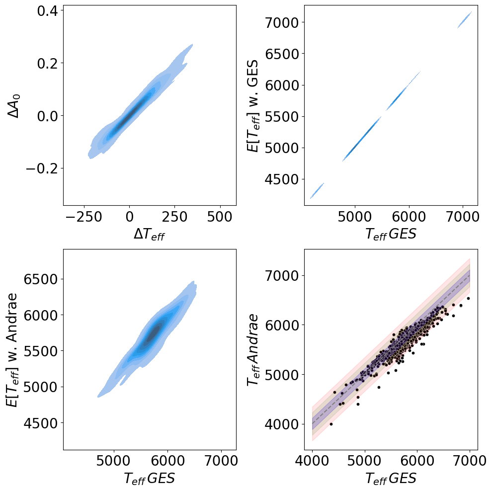
Figure 17: The difference in mean extinction and mean temperature as calculated by using the AAP and using the GES stellar parameters as constraints. The top-left plot shows that when the mean extinction differs ($\Delta A_{0}$) using AAP vs GES estimates of the effective temperature there is a corresponding difference in the posterior mean effective temperature ($\Delta T_{\text{eff}}$), due to the degeneracy between the two parameters. The top right plot shows the posterior mean effective temperature when using a GES effective temperature as a constraint versus the constraint value itself. The bottom-left image shows the posterior mean effective temperature using the AAP constraint on the effective temperature temperature versus the GES effective temperature constraint. The bottom-right plot shows the AAP effective temperature versus the GES value, the blue hue indicates a $\sigma=110$ K band from the line $y=x$.

5.5 Dust Map Comparison

We wish to use a well-studied region and run our full method, including all necessary cuts, to derive a map of extinction and compare it with other dust maps. We select a square region of width $3^{\circ}$ region centred on $l=104^{\circ}$ and $b=22.5^{\circ}$ which has been studied in Panopoulou et al. (2019) by the PASIPHAE team (Tassis et al., 2018), where they show that the polarization signal is a tracer of two large clouds in the sightline, each at varying distances. Figure 1 in Panopoulou et al. (2019) shows the H1 emission maps of the region.

We query the Gaia database and cross-match with 2MASS, and ALLWISE in the same manner as described throughout the previous sections. We make all the necessary cuts described before and then run our model to generate samples from the posterior. We take the mean extinction value and carry out the Gaussian smoothing process as described in Section 4.9.

In Figure 18 we display our dust map generated using a full solution (top-left plot) assuming an exponential prior on $A_{0}$ with $\lambda=5$ and a floor error of $0.05$ mag. In the top-right plot, we show the HI emission map from Lenz et al. (2017). Moreover, we compare these dust maps with the Planck extinction map (Planck Collaboration et al., 2016) (bottom-left) and the Bayestar (Green et al., 2018) dust map (bottom-right) for the same region. Each of the extinction values is on a different scale and we apply a standard normal Z transformation to the mean extinctions and then apply a min-max scaler so the values lie between 0 and 1. We calculate a residual between our dust map using the full solution and the other dust maps by finding the absolute difference $|\Delta A_{0}|$ for the scaled extinction at each point of the dust map. We display the residuals in Figure 19.

We see there is a high correlation between our full solution dust map and the dust map generated by Bayestar. In particular the region of high extinction between $103.0<l<104.5$ at the bottom of our dust map is present in both maps (and indeed the other maps as well). Moreover, there is a correlation between our dust map and the Baystar dust map for regions of high extinction and low extinction. By looking at the residuals we see that there is a significant feature in the Planck map that is not present in the other maps. This is because the Planck map has been integrated to infinity, whereas our dust map and the Bayestar dust map both use radial distance and we have not probed distances to reach the cloud, which we know from Panopoulou et al. (2019).

Another key feature of the dust clouds mentioned in Panopoulou et al. (2019) is the circular type cloud bounded by $104<l<104.5$ and $22.05<b<23.0$, which can be seen vaguely in the Planck dust map. We note that our method shows some relatively low extinction in this region, but does not reproduce the same topology as the Planck map.

It is important to note that our dust maps have been generated using the mean value of the extinction posterior. From the discussions in this paper, we expect that regions of high extinction will appear as regions of high extinction using just the mean value. But regions of low extinction can give a relatively large mean value of the extinction too, generating artificial structure in the dust map. We can see this is particularly true in the case when we use photometry and parallax only. Without a good prior on the extinction parameter, $A_{0}$, we expect the posterior to be very wide for each star, and therefore the mean to be large. As these artificially large representations of the extinction get smoothed spatially, we generate false, artificial structures. Hence, to detect fine variation in the ISM, we will need to use the full posterior distribution of extinction.

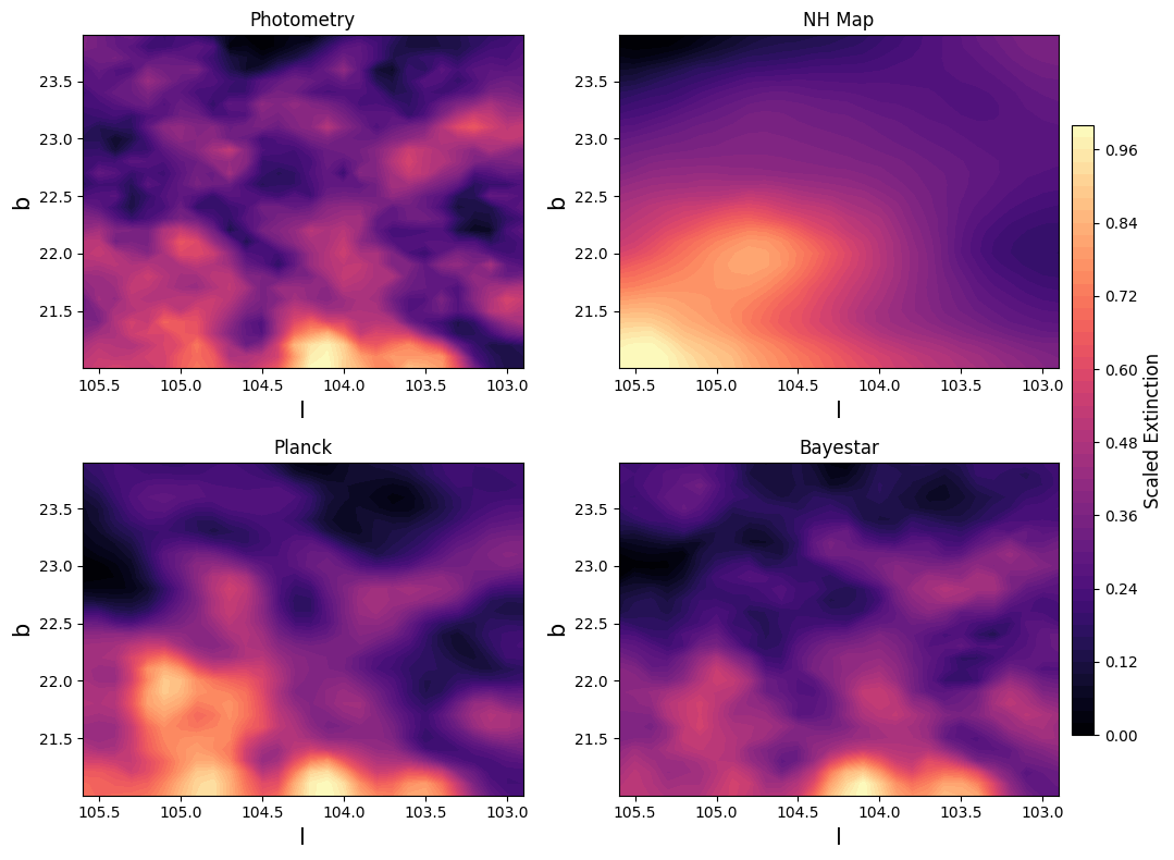
Figure 18: Comparison between dust maps of a $3^{\circ}$ Region Centered at Galactic Coordinates $l=104^{\circ}$ and $b=22.5^{\circ}$, as studied by the PASIPHAE team in 2019. Panopoulou et al. (2019) have studied this region to show HI maps trace two different clouds at different distances. The top-left image is our dust map generated by smoothing over the posterior mean extinction using photometry, parallax and an effective temperature estimate. The top-right image shows the HI emission for the region. The bottom-left image shows the Planck dust map for the same region, and the bottom-right shows the Bayestar dust map for the same region. The topology of each dust map is complex due to smoothing effects.

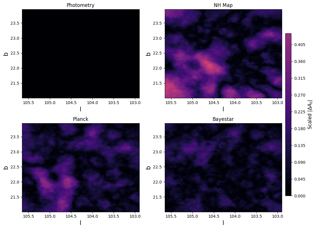
Figure 19: Comparison of the residuals between our full solution dust map and the other dust maps, for a $3^{\circ}$ Region Centered at Galactic Coordinates $l=104^{\circ}$ and $b=22.5^{\circ}$, as described in Figure 18. The hue is the absolute difference between the dust maps, scaled between 0 and 1. Here we see that there is significant agreement between our dust map and the Bayestar dust map. Moreover, by looking at the residuals, we can see the cloud in the bottom-left of the Planck dust map which we know is outside the region we have probed.

6 Conclusions

This paper illustrates the complexities which arise when charting low variations in extinction for high Galactic latitude sightlines. We developed a Bayesian model to identify a region of the Hertzsprung-Russell diagram suited to constrain the single-star extinction accurately at high Galactic latitudes. Using photometry from Gaia, 2MASS and ALLWISE together with parallax from Gaia, we employ nested sampling to fit the model to the data and analyse the posterior over stellar parameters for both synthetic and real data. The main conclusions are as follows.

• Tracing small variations in the ISM at high Galactic latitudes requires a careful posterior analysis of stars and their properties that affect the extinction posterior.

• The degeneracy between extinction and other stellar parameters (in particular, the effective temperature) requires a full posterior over the parameters as the solution to deriving low variation in the extinction parameter.

• Introducing prior constraints on the metallicity, the effective temperature, and/or the extinction will significantly restrict the extinction posterior.

• One has to be careful in choosing such priors. The significant degeneracy means any statement about the effective temperature is a statement about the extinction, and vice versa. If prior assumptions are incompatible, or too narrow, one derives a non-physical extinction posterior.

• The inaccuracies in the stellar models have a significant impact on constraining the true extinction. Calibration against independent, highly accurate effective temperatures for stars at high Galactic latitudes will constrain the systematic inaccuracies. We propose a cut in Gaia absolute magnitudes, $4.0<M_{G}<8$, where the stellar models are the most accurate and the systematic effects are minimised.

• The extinction-effective temperature degeneracy allows for a family of point estimate pairs of $(T_{eff},A_{0})$, for a single star at high Galactic latitudes, which achieve a similar posterior probability. One can fit a curve to the right plot in Figure 12 to convert a pair to another equally likely pair with different extinction.

• The non-linearity of this relation is important for comparing effective temperatures from different surveys. Effective temperatures can appear to be substantially different. However, this can happen due to different assumptions about the underlying extinction and both solutions can be equally probable under the posterior distribution.

• Outliers, such as binary systems or young stars, can appear to have significantly higher extinction than other stars in the sample. If these stars are binned into sightlines to derive extinctions they can cause the extinction of the sight-line to be skewed. Flagging these stars is important when we wish to constrain small variations in the ISM.

• Without enforcing spatial smoothing in our posterior analysis, we can reconstruct similar dust maps to current benchmarks for high Galactic latitude regions.

• The dust map uses only the extinction posterior mean for each star and generates significant artificial structure on small scales. One must use the full posterior to quantify the detection of the ISM for small variations.

Data Availability

This study uses data from Gaia DR3 (Gaia Collaboration et al., 2022), 2MASS (Cutri et al., 2003) and ALLWISE (Cutri et al., 2013), all of which are publicly available. Moreover, the stellar parameters estimates used throughout come from Andrae et al. (2023), LAMOST DR8 (Wang, 2022) and Gaia-ESO (Gilmore et al., 2022), which are all publicly available.

Appendix A Degeneracies Arising in SED Fitting

In this section, we discuss the parameter degeneracies and how they are inherent to the synthetic Spectral Energy Distribution (SED) used to fit for the stellar parameters. In particular, we show that the extinction-effective temperature degeneracy is more prominent for low values of extinction and the more of the SED we observe the better we can constrain extinction. Moreover, we find that without an assumption of the underlying stellar evolution, another strong degeneracy arises between the extinction and the radius. These results differ depending on the stellar parameters themselves, here we show the case of solar-type stars.

To illustrate these points we use the PHOENIX (Husser et al., 2013) grid of synthetic spectra resampled to a spectral resolving power of $\lambda/\Delta\lambda=720$, and the (Fitzpatrick, 1999) extinction law with $R_{V}=3.1$ to generate synthetic fluxes at different wavelengths over a grid of stellar parameters. We define our grid by setting $\log(g)=4.5$ dex and allowing the effective temperature, metallicity and extinction range between $3500\text{ K}<T_{\text{eff}}<8000\text{ K}$, $-2.5\text{ dex}<[Fe/H]<0.5\text{ dex}$, and $0<A_{0}<2$, respectively. For values not defined by the original PHOENIX grid we perform cubic interpolation over grid points to generate fluxes at the given wavelengths for the corresponding grid point. This defines a vector function $\textbf{f}=f([Fe/H],T_{eff},\log(g),A_{0})$, which outputs fluxes at a set of fixed wavelength points. We set a lower bound of the wavelengths to be the Lyman limit, $912$ Å and an upper bound of $65,000$ Å (larger than the upper bound of the W1 and W2 passband filters). Throughout, we will resample the spectra to a number of wavelength observations to investigate how different observations of the SED affect the accuracy we can recover extinction.

We illustrate the degeneracies which arise in fitting the synthetic spectra, $\textbf{f}=f([Fe/H],T_{eff},\log(g),A_{0})$, to an observed spectrum, $\hat{\textbf{f}}$, sampled at the same wavelengths under a Gaussian likelihood function with error covariance matrix $\boldsymbol{\Sigma}$ arising from the measurement error of the flux at each wavelength. We can find estimates of the parameter covariances for the maximum likelihood estimate using the Fisher information matrix. Throughout, we assume the measurement error of the flux at each point constitutes the Gaussian covariance matrix $\boldsymbol{\Sigma}=\hat{\textbf{F}}\times(2\log_{e}(10)(0.01)/5)^{2}$, where F is the diagonal matrix with $\hat{F}_{ii}=\hat{f}_{i}^{2}$. This flux error corresponds to a constant photometric magnitude error of $0.01$ mag. Fixing all parameters except two, $\alpha$ and $\beta$, the Fisher information matrix $I$ is given by the components $I_{\alpha,\beta}=\frac{\partial\textbf{f}}{\partial\alpha}^{T}\boldsymbol{\Sigma}^{-1}\frac{\partial\textbf{f}}{\partial\beta}$. If we define $\boldsymbol{C}=I^{-1}$, we introduce covariances for the parameters which, for the maximum likelihood estimate, satisfy the Cramer Rao lower bound. Thus, we define $\sigma(\alpha)=\sqrt{C_{\alpha,\alpha}}$ and $\rho(\alpha,\beta)=C_{\alpha,\beta}/{\sigma(\alpha)\sigma(\beta)}$, as the standard deviation of the parameter $\alpha$ and the correlation between parameters, respectively.

We inspect the extinction-effective temperature degeneracy using the methods above and we found two key points. Firstly, for a fixed measurement error observing fewer fluxes reduces the ability to constrain the effective temperature and extinction. Thus, increasing the number of passband filters and independent observations in ones analysis will provide a better estimate of the extinction. Secondly, the correlation between extinction and effective temperature is present across all parameter ranges, however, at high extinctions the introduction of longer wavelength observations disentangles the degeneracy between the two parameters, this is a well-known effect and has been noted in (Bailer-Jones, 2011). The introduction of the near-to-far IR wavelength observations will put a ceiling on the large values of extinction that provide a good fit to the data. However, for small values of extinction, the longer wavelength flux observations do not have the same effect in identifying the difference between extinction and effective temperature. If we have prior knowledge that extinction is low, observations in the optical are far more valuable in constraining the extinction and effective temperature, respectively.

We fix $[Fe/H]=0$ dex and $\log(g)=4.5$ dex to inspect the relationship between the effective temperature and the extinction parameter for a solar-type star. We evaluate $\textbf{f}=f([Fe/H],T_{eff},\log(g),A_{0})$ at effective temperatures between $3500\text{ K}<T_{\text{eff}}<8000\text{ K}$, in $10$ K steps, and extinctions between $0<A_{0}<2$, in $0.02$ steps. We analyse the results using $2000$, $40$ and $15$ wavelength observations. We find that the correlation between extinction and effective temperature is largely present across all parameters in this example. However, at lower extinctions the degeneracy has more of an influence on constraining the effective temperature and extinction, this is because, for low extinctions, the extinction curve has an extremely small effect on the long wavelength observations. Moreover, decreasing the number of flux observations reduces the accuracy of constraining both parameters. We show how a smaller value of extinction exhibits a larger degeneracy to the effective temperature in Figure 20 than when the extinction is higher (Figure 21).

We conduct a similar experiment to investigate the relationship between the metallicity and the effective temperature (and, therefore, the extinction). We display these results by first fixing $A_{0}=0.1$ dex and $\log(g)=4.5$ dex to inspect the relationship between the effective temperature and the metallicity. We evaluate $\textbf{f}=f([Fe/H],T_{eff},\log(g),A_{0})$ at effective temperatures between $3500\text{ K}<T_{\text{eff}}<8000\text{ K}$, in $10$ K steps, and metallicity between $-2.5<[Fe/H]<0.5$, in $0.02$ dex steps. We find that the degeneracy between the metallicity and effective temperature (and extinction) increases across the parameter ranges with a decreasing number of wavelength observations. This happens because the fewer observations we have the effects of absorption lines and other metallicity-dependent properties are smoothed over, making it more difficult to uniquely identify the SED to a given metallicity.

The effective temperature (and the extinction) is degenerate with the stellar radius and constraining the stellar radius either through stellar evolution theory or other means is necessary to constrain the extinction. We fix $[Fe/H]=0$ dex, $\log(g)=4.5$ dex, and $A_{0}=0.1$ to inspect the relationship between the effective temperature and the radius parameter for a solar-type star. We evaluate $\textbf{f}=f([Fe/H],T_{eff},\log(g),A_{0})R^{2}$ at effective temperatures between $3500\text{ K}<T_{\text{eff}}<8000\text{ K}$, in $10$ K steps, and stellar radii, $R$, between $0.1R_{\odot}<R<100R_{\odot}$, in $0.5R_{\odot}$ steps. The extent of the influence of the degeneracy on the effective temperature (and extinction) depends on how large the radius is. Thus, having a prior constraint on the stellar radius will allow a tighter constraint on the extinction.

Using ether the PHOENIX (Husser et al., 2013) synthetic atmosphere, the ATLAS9 synthetic atmosphere models (Castelli & Kurucz, 2004) or any other synthetic model introduces some bias as there are inconsistencies which arise in the synthetic fluxes for a given set of stellar parameters. Due to the parameter degeneracies, if one uses different stellar atmosphere models under an extinction assumption they can derive different values of stellar parameters from the observed SED. We look for relative differences in extinction so we must fix our grid of atmosphere models.

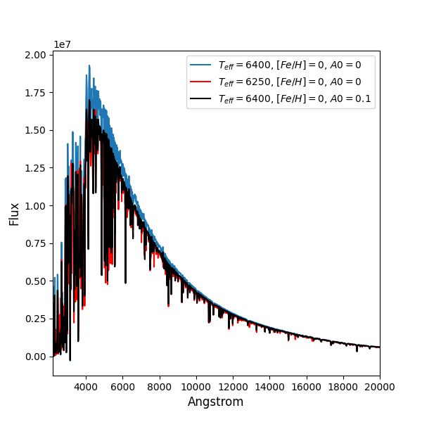
Figure 20: Three solar metallicity SEDs of varying effective temperature and extinction. We see that, for a small amount of extinction $A_{0}=0.1$, we can find a similar SED corresponding to a zero extinction star with a different effective temperature. In particular, when we integrate over passbands this becomes increasingly difficult.

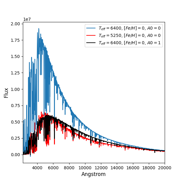
Figure 21: Three solar metallicity SEDs of varying effective temperature and extinction. We see that for a relatively large amount of extinction $A_{0}=1$, the degeneracy between extinction and effective temperature is not as pronounced. It is easier to detect the difference between the effective temperature and extinction for high extinction regions when one has observations of the flux at longer wavelengths.

Appendix B Using Pan-STARRS Data

It is well known that the wide passbands in the optical, such as Gaia’s, have temperature-dependent extinction coefficients (Zhang & Yuan, 2022). In this section, we show that under ideal measurement error conditions and assuming no systematic effects are introduced, using narrower passbands in optical wavelength ranges will partially narrow the extinction posterior.

We illustrate this by performing synthetic analysis using the grizy passband filter from the highly accurate Panoramic Survey Telescope and Rapid Response System 1 (Pan-STARRS, Chambers et al. (2016)) which is a 1.8 m optical and near-infrared telescope located in Hawaii, USA. The mean $5\sigma$ point source limiting sensitivities in the stacked $3\pi$ Steradian Survey in grizy are (23.3, 23.2, 23.1, 22.3, 21.4) respectively. The upper bound on the systematic uncertainty in the photometric calibration across the sky is 7-12 millimag depending on the bandpass. We synthesise the photometry in the same manner as described in Section 3 by using the passband definitions as described in Tonry et al. (2012).

To understand how the Pan-STARRS passbands influence the extinction posterior we generate the identical uniform sample as described in Section 4.2, however, we also include synthetic photometry for the grizy passbands and add extinction in these passbands using the Fitzpatrick (1999) extinction law with $A_{0}=0.15$. The error on the photometric magnitudes in the new passbands is synthesised in the same manner as the other passbands as described in Section 4.2. That is, we model the measurement error using real data from a high Galactic sample.

We fit our model to the data by assuming uniform priors on the metallicity and the extinction parameter (in the same manner as Section 4.3). Moreover, we assume all photometric magnitudes have a floor error of $0.05$ mag. We recall from Table 2 that without using Pan-STARRS photometry the median difference between the posterior mean extinction and the true value of $A_{0}=0.15$ is $0.206$. When we fit our model to the data including the Pan-STARRS photometric magnitudes, we find a median difference between the posterior mean and the true value of $0.128$. However, the distance becomes less pronounced when we incorporate metallicity and extinction priors.

We stress that the key results from the paper are independent of using the Pan-STARRS data. However, using any extra photometric passbands that are well calibrated, such as Pan-STARRS, will help us constrain the SED of a star and therefore provide useful information in further constraining the extinction posterior. If we wish to chart very small variations in extinction Pan-STARRS will be useful due to the accuracy of its’ photometry and the density of the survey. To conclude we present a plot of the errors derived from the uniform sample both with and without using Pan-STARRS data in Figure 22

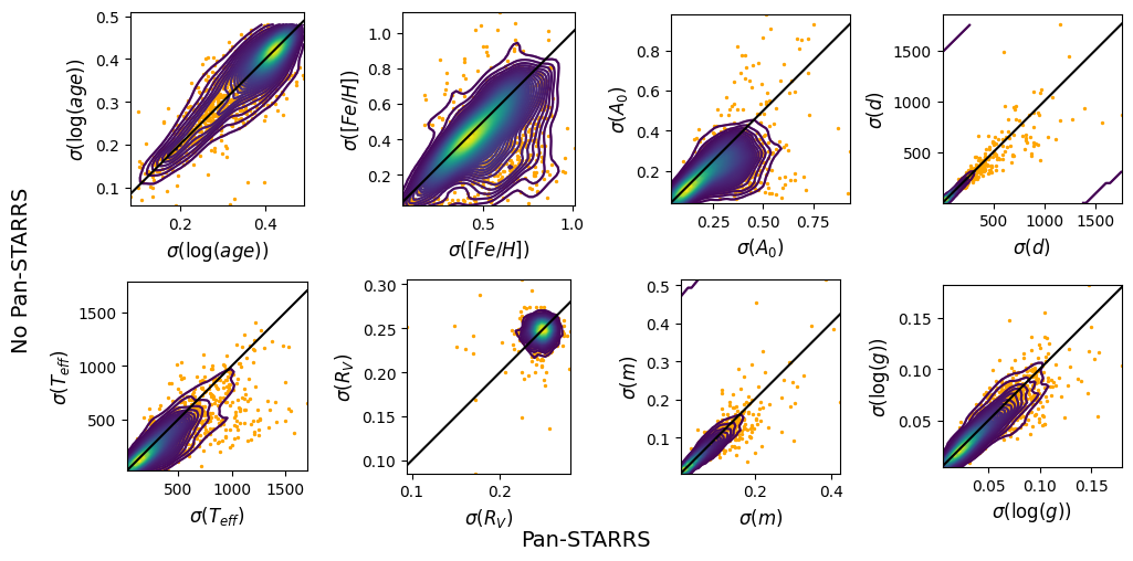
Figure 22: Scatter plot of posterior standard deviation for each parameter over the uniform sample described in Section 4.2 when using uniform priors and (horizontal axis) using the Pan-STARRS data and (vertical axis) not using the Pan-STARRS data.

Appendix C Low Effective Temperature Offset in APOGEE

It has been noted in the literature that the APOGEE (Jönsson et al., 2020) spectroscopic effective temperature estimates disagree with other surveys, often attributed to an incorrect extinction estimate (Hegedűs et al., 2023). In this section, we show that both LAMOST and APOGEE provide effective temperatures which are consistent with each other, even within the range of disputed effective temperatures, in the sense that we can use the relation in the right plot of Figure 12 to transform a certain amount of extinction into an effective temperature correction term to reproduce the LAMOST effective temperatures and the APOGEE effective temperatures.

We use the sample we generated in Section 5.1, which was generated by cross-matching high Galactic latitude sources from LAMOST with APOGEE, Gaia, 2MASS and ALLWISE. Therein, we showed that we could generate effective temperatures consistent with LAMOST by finding the effective temperatures consistent with a zero extinction solution. We find that taking an extinction contribution of $\delta A_{0}=0.15$ and finding the effective temperatures corresponding to a global reduction of this extinction provides a good fit between the transformed effective temperatures and those derived by APOGEE.

Subtracting this contribution, we find a median difference between our transformed mean posterior effective temperatures and their effective temperatures to be $0.17$ K. The mean difference is $28.3$ K. It is important to note that we can reliably transform between the APOGEE and the LAMOST effective temperatures using this relation. The zero point of extinction in both of these cases is different due to prior assumptions, but they both achieve indistinguishable probabilities under the full posterior distribution. We present an illustration of these results in Figure 23.

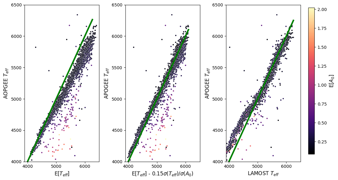
Figure 23: Illustrating APOGEE and LAMOST effective temperatures have the same posterior probability. In Section 5.1 we showed that we could extinction-correct our mean effective temperature to derive the LAMOST effective temperatures, both values had similar posterior probabilities. From the left, the image shows the effective temperatures derived from APOGEE versus the unaltered posterior mean effective temperature for each point in the sample. The middle plot shows the transformation using the zero-point extinction, which best fits the transformed effective temperature and the APOGEE effective temperatures. This amounts to subtracting $\delta A_{0}=0.15$ amount of extinction from the posterior mean effective temperature. The right plot shows the APOGEE effective temperatures versus LAMOST effective temperatures, unaltered by extinction.

References

- Andrae et al. (2022) Andrae R., et al., 2022, arXiv e-prints, p. arXiv:2206.06138
- Andrae et al. (2023) Andrae R., Rix H.-W., Chandra V., 2023, The Astrophysical Journal Supplement Series, 267, 8
- Bailer-Jones (2011) Bailer-Jones C. A. L., 2011, MNRAS, 411, 435
- Bailer-Jones et al. (2021) Bailer-Jones C. A. L., Rybizki J., Fouesneau M., Demleitner M., Andrae R., 2021, The Astronomical Journal, 161, 147
- Bressan et al. (2012) Bressan A., Marigo P., Girardi L., Salasnich B., Dal Cero C., Rubele S., Nanni A., 2012, MNRAS, 427, 127
- Buchner (2021) Buchner J., 2021, UltraNest – a robust, general purpose Bayesian inference engine (arXiv:2101.09604)
- Buchner (2023) Buchner J., 2023, Statistics Surveys, 17
- Cardelli et al. (1989) Cardelli J. A., Clayton G. C., Mathis J. S., 1989, ApJ, 345, 245
- Castelli & Kurucz (2004) Castelli F., Kurucz R. L., 2004, New Grids of ATLAS9 Model Atmospheres (arXiv:astro-ph/0405087)
- Chabrier (2003) Chabrier G., 2003, PASP, 115, 763
- Chambers et al. (2016) Chambers K. C., et al., 2016, arXiv e-prints, p. arXiv:1612.05560
- Choi et al. (2016a) Choi J., Dotter A., Conroy C., Cantiello M., Paxton B., Johnson B. D., 2016a, The Astrophysical Journal, 823, 102
- Choi et al. (2016b) Choi J., Dotter A., Conroy C., Cantiello M., Paxton B., Johnson B. D., 2016b, ApJ, 823, 102
- Cohen et al. (2003) Cohen M., Wheaton W. A., Megeath S. T., 2003, AJ, 126, 1090
- Cutri et al. (2003) Cutri R. M., et al., 2003, 2MASS All Sky Catalog of point sources.
- Cutri et al. (2013) Cutri R. M., et al., 2013, Explanatory Supplement to the AllWISE Data Release Products, Explanatory Supplement to the AllWISE Data Release Products, by R. M. Cutri et al.
- Du et al. (2016) Du B., et al., 2016, ApJS, 227, 27
- Edenhofer et al. (2023) Edenhofer G., Zucker C., Frank P., Saydjari A. K., Speagle J. S., Finkbeiner D., Enßlin T., 2023, arXiv e-prints, p. arXiv:2308.01295
- Fabricius et al. (2021) Fabricius C., et al., 2021, A&A, 649, A5
- Feroz et al. (2009) Feroz F., Hobson M. P., Bridges M., 2009, Monthly Notices of the Royal Astronomical Society, 398, 1601
- Fitzpatrick (1999) Fitzpatrick E. L., 1999, PASP, 111, 63
- Gaia Collaboration et al. (2016) Gaia Collaboration et al., 2016, A&A, 595, A1
- Gaia Collaboration et al. (2022) Gaia Collaboration et al., 2022, arXiv e-prints, p. arXiv:2208.00211
- Gilmore et al. (2022) Gilmore G., et al., 2022, A&A, 666, A120
- Grayson et al. (2016) Grayson J. A., et al., 2016, in Holland W. S., Zmuidzinas J., eds, Society of Photo-Optical Instrumentation Engineers (SPIE) Conference Series Vol. 9914, Millimeter, Submillimeter, and Far-Infrared Detectors and Instrumentation for Astronomy VIII. p. 99140S (arXiv:1607.04668), doi:10.1117/12.2233894
- Green et al. (2018) Green G. M., et al., 2018, MNRAS, 478, 651
- Green et al. (2019) Green G. M., Schlafly E., Zucker C., Speagle J. S., Finkbeiner D., 2019, ApJ, 887, 93
- Handley et al. (2015) Handley W. J., Hobson M. P., Lasenby A. N., 2015, MNRAS, 450, L61
- Hastings (1970) Hastings W. K., 1970, Biometrika, 57, 97
- Hegedűs et al. (2023) Hegedűs V., Mészáros S., Jofré P., Stringfellow G. S., Feuillet D., García-Hernández D. A., Nitschelm C., Zamora O., 2023, A&A, 670, A107
- Hidalgo et al. (2018) Hidalgo S. L., et al., 2018, ApJ, 856, 125
- Husser et al. (2013) Husser T. O., Wende-von Berg S., Dreizler S., Homeier D., Reiners A., Barman T., Hauschildt P. H., 2013, A&A, 553, A6
- Jönsson et al. (2020) Jönsson H., et al., 2020, AJ, 160, 120
- Kirkpatrick et al. (2016) Kirkpatrick J. D., et al., 2016, The Astrophysical Journal Supplement Series, 224, 36
- Lallement et al. (2019) Lallement R., Babusiaux C., Vergely J. L., Katz D., Arenou F., Valette B., Hottier C., Capitanio L., 2019, A&A, 625, A135
- Lenz et al. (2017) Lenz D., Hensley B. S., Doré O., 2017, The Astrophysical Journal, 846, 38
- Li & Draine (2001) Li A., Draine B. T., 2001, ApJ, 554, 778
- Lindegren et al. (2021a) Lindegren L., et al., 2021a, A&A, 649, A4
- Lindegren et al. (2021b) Lindegren L., et al., 2021b, Astronomy & Astrophysics, 649, A4
- Mainzer et al. (2011) Mainzer A., et al., 2011, ApJ, 731, 53
- Mandel et al. (2022) Mandel K. S., Thorp S., Narayan G., Friedman A. S., Avelino A., 2022, MNRAS, 510, 3939
- Marigo et al. (2017) Marigo P., et al., 2017, The Astrophysical Journal, 835, 77
- Marrese et al. (2022) Marrese P. M., Marinoni S., Fabrizio M., Altavilla G., 2022, Gaia DR3 documentation Chapter 15: Cross-match with external catalogues, Gaia DR3 documentation, European Space Agency; Gaia Data Processing and Analysis Consortium.
- Mudur et al. (2023) Mudur N., Park C. F., Finkbeiner D. P., 2023, The Astrophysical Journal, 949, 47
- Panopoulou et al. (2019) Panopoulou G. V., et al., 2019, The Astrophysical Journal, 872, 56
- Peek & Schiminovich (2013) Peek J. E. G., Schiminovich D., 2013, ApJ, 771, 68
- Planck Collaboration et al. (2016) Planck Collaboration et al., 2016, A&A, 596, A109
- Queiroz et al. (2018) Queiroz A. B. A., et al., 2018, MNRAS, 476, 2556
- Randich et al. (2022) Randich S., et al., 2022, A&A, 666, A121
- Riello et al. (2021) Riello M., et al., 2021, VizieR Online Data Catalog, pp J/A+A/649/A3
- Schlegel et al. (1998) Schlegel D. J., Finkbeiner D. P., Davis M., 1998, ApJ, 500, 525
- Skilling (2004) Skilling J., 2004, in Fischer R., Preuss R., Toussaint U. V., eds, American Institute of Physics Conference Series Vol. 735, Bayesian Inference and Maximum Entropy Methods in Science and Engineering: 24th International Workshop on Bayesian Inference and Maximum Entropy Methods in Science and Engineering. pp 395–405, doi:10.1063/1.1835238
- Skrutskie et al. (2006) Skrutskie M. F., et al., 2006, The Astronomical Journal, 131, 1163
- Speagle (2020) Speagle J. S., 2020, MNRAS, 493, 3132
- Tassis et al. (2018) Tassis K., et al., 2018, PASIPHAE: A high-Galactic-latitude, high-accuracy optopolarimetric survey (arXiv:1810.05652)
- Tonry et al. (2012) Tonry J. L., et al., 2012, ApJ, 750, 99
- Wang (2022) Wang 2022, ApJS, 259, 51
- Wright et al. (2010) Wright E. L., et al., 2010, The Astronomical Journal, 140, 1868
- Wu et al. (2014) Wu Y., Du B., Luo A., Zhao Y., Yuan H., 2014. pp 340–342 (arXiv:1407.1980), doi:10.1017/S1743921314010825
- Zhang & Yuan (2022) Zhang R., Yuan H., 2022, The Astrophysical Journal Supplement Series, 264, 14
- Zhang et al. (2023a) Zhang R., Yuan H., Chen B., 2023a, A Rv map of the Milky Way revealed by LAMOST (arXiv:2309.04113)
- Zhang et al. (2023b) Zhang X., Green G. M., Rix H.-W., 2023b, arXiv e-prints, p. arXiv:2303.03420