Safe Control for Soft-Rigid Robots with Self-Contact
using Control Barrier Functions

Abstract

Incorporating both flexible and rigid components in robot designs offers a unique solution to the limitations of traditional rigid robotics by enabling both compliance and strength. This paper explores the challenges and solutions for controlling soft-rigid hybrid robots, particularly addressing the issue of self-contact. Conventional control methods prioritize precise state tracking, inadvertently increasing the system’s overall stiffness, which is not always desirable in interactions with the environment or within the robot itself. To address this, we investigate the application of Control Barrier Functions (CBFs) and High Order CBFs to manage self-contact scenarios in serially connected soft-rigid hybrid robots. Through an analysis based on Piecewise Constant Curvature (PCC) kinematics, we establish CBFs within a classical control framework for self-contact dynamics. Our methodology is rigorously evaluated in both simulation environments and physical hardware systems. The findings demonstrate that our proposed control strategy effectively regulates self-contact in soft-rigid hybrid robotic systems, marking a significant advancement in the field of robotics.

I Introduction

As the soft robotics field continues its growth towards maturity, there is a nascent trend towards soft-rigid hybrid robot forms to allow both compliance for safe operation in uncertain environments and rigidity to allow load bearing capability [1, 2, 3, 4]. Indeed, the majority of terrestrial life forms have some articulated rigid body structure that allows self-support under gravity. Such robots may expand the range of potential behaviors of robots, but they also may instantiate in new problems. In this work, we will look at a class of soft-rigid robots that frequently undergo rigid self contact and we will seek to control these systems to gracefully deal with self contact.

While the field of soft robotic control has experienced rapid growth over the past decade [5], critical open questions remain. Thus far, most works have focused on precise state [6] or end-effector tracking [7], yet these tasks may ultimately be incidental to the goals of soft robots. This is because, as discussed in [8], there is a trade-off between feedback and stiffness, with more feedback increasing the effective stiffness of the system, eliminating the benefits of soft materials. Feedforward control does not suffer the same issues, but requires precise models that are fundamentally difficult for soft robots. Thus, while balanced feedforward plus feedback controllers like the PD+ controller have been shown to stabilize state trajectories for soft robots [5], this comes at a cost of stiffening the robot’s potential interactions with the environment (or with itself in self-contact), and a similar problem is bound to occur for end-effector tracking control as well. This motivates exploration of alternative methods of certifying performance for soft robots, ones that do not necessitate asymptotic convergence to a trajectory. Inspired by the the above discussion, and by the safety requirements of soft-rigid articulated robots discussed previously, we explore formal guarantees in operation with the use of Control Barrier Functions (CBFs) to govern their behavior.

Barrier Functions (BFs) are Lyapunov-like functions [9, 10] whose use can be traced back to optimizations [11], in which case they are added in objective functions. Their primary use is to enforce constraints while doing optimization. Control Barrier Functions (CBFs) represent an extension of BFs tailored for control systems. They transform a constraint defined in terms of system states into a constraint on the control inputs. CBFs offer a state-feedback controller that is rigorously proven to be safe while remaining computationally efficient. Specifically, CBFs are well-suited for constraints characterized by a relative degree of one concerning the system dynamics [12, 13]. The High Order CBF (HOCBF), as proposed in [14], is designed to effectively handle constraints with arbitrarily high relative degrees, making it a versatile extension of the conventional CBF framework.

For soft-rigid robots that experience self-contact, CBFs provide a natural mechanism to design controllers that can gracefully regulate behavior near contact points (they have previously been used for something similar with humanoids [15]). They also naturally encapsulate other constraints common in continuum robots, such as limits to extension. More generally for soft and interactive robots, CBFs provide a mechanism of safety and performance verification that can be used to guarantee properties without relying on asymptotically stable control of the state of the robot. In this work, we adopt the commonly-used Piecewise Constant Curvature (PCC) model for our system. To our knowledge, this is the first work applying CBFs to PCC models.

In summary, we contribute a methodology for controlling serial soft-rigid hybrid robots that undergo self-contact. Additionally, we contribute the first use of Control Barrier Functions for governing the behavior of continuum robots.

II Preliminaries and System Formulation

Figure 1: An example of the type of hardware we examine for this work, where the modular soft-rigid segments frequently make self contact. We seek to operationalize representations of distance functions such as $c_{j}$ to gracefully control such structures in the presence of self contact using CBFs.

II-A High Order CBFs

We briefly introduce the concept of high order CBFs in this section, and we start with some definitions for CBFs/HOCBFs.

Definition 1

(Class $\mathcal{K}$ function [16]) A continuous function $\alpha:[0,a)\rightarrow[0,\infty),a>0$ is said to belong to class $\mathcal{K}$ if it is strictly increasing and $\alpha(0)=0$. A continuous function $\beta:\mathbb{R}\rightarrow\mathbb{R}$ is said to belong to extended class $\mathcal{K}$ if it is strictly increasing and $\beta(0)=0$.

Consider an affine control system of the form:

$$\dot{\bm{x}}=f(\bm{x})+g(\bm{x})\bm{u}$$ (1)

where $\bm{x}\in X\subset\mathbb{R}^{n}$, $f:\mathbb{R}^{n}\rightarrow\mathbb{R}^{n}$ and $g:\mathbb{R}^{n}\rightarrow\mathbb{R}^{n\times q}$ are Lipschitz continuous, and $\bm{u}\in U\subset\mathbb{R}^{q}$ is the control constraint set defined as ($\bm{u}_{min},\bm{u}_{max}\in\mathbb{R}^{q}$):

$$U:=\{\bm{u}\in\mathbb{R}^{q}:\bm{u}_{min}\leq\bm{u}\leq\bm{u}_{max}\},$$ (2)

where the inequalities are interpreted element-wise.

Definition 2

A set $C\subset\mathbb{R}^{n}$ is forward invariant for system (1) if its solutions for some $\bm{u}\in U$ starting at any $\bm{x}(0)\in C$ satisfy $\bm{x}(t)\in C,$ $\forall t\geq 0$.

Definition 3

(Relative degree [16]) The relative degree of a (sufficiently many times) differentiable function $b:\mathbb{R}^{n}\rightarrow\mathbb{R}$ with respect to system (1) is the number of times it needs to be differentiated along its dynamics until any component of the control $\bm{u}$ explicitly shows in the corresponding derivative.

Since function $b$ is used to define a constraint $b(\bm{x})\geq 0$, we will also refer to the relative degree of $b$ as the relative degree of the constraint. For a constraint $b(\bm{x})\geq 0$ with relative degree $m$, $b:\mathbb{R}^{n}\rightarrow\mathbb{R}$, and $\psi_{0}(\bm{x}):=b(\bm{x})$, we define a sequence of functions $\psi_{i}:\mathbb{R}^{n}\rightarrow\mathbb{R},i\in\{1,\dots,m\}$:

$$\psi_{i}(\bm{x}):=\dot{\psi}_{i-1}(\bm{x})+\alpha_{i}(\psi_{i-1}(\bm{x})),i\in\{1,\dots,m\},$$ (3)

where $\alpha_{i}(\cdot),i\in\{1,\dots,m\}$ denotes a $(m-i)^{th}$ order differentiable class $\mathcal{K}$ function.

We further define a sequence of sets $C_{i},i\in\{1,\dots,m\}$ associated with (3) in the form:

$$C_{i}:=\{\bm{x}\in\mathbb{R}^{n}:\psi_{i-1}(\bm{x})\geq 0\},i\in\{1,\dots,m\}.$$ (4)

Definition 4

(High Order Control Barrier Function (HOCBF) [14]) Let $C_{1},\dots,C_{m}$ be defined by (4) and $\psi_{1}(\bm{x}),\dots,\psi_{m}(\bm{x})$ be defined by (3). A function $b:\mathbb{R}^{n}\rightarrow\mathbb{R}$ is a High Order Control Barrier Function (HOCBF) of relative degree $m$ for system (1) if there exist $(m-i)^{th}$ order differentiable class $\mathcal{K}$ functions $\alpha_{i},i\in\{1,\dots,m-1\}$ and a class $\mathcal{K}$ function $\alpha_{m}$ such that

$$\sup_{\bm{u}\in U}[L_{f}^{m}b(\bm{x})+L_{g}L_{f}^{m-1}b(\bm{x})\bm{u}+O(b(\bm{x}))$$ (5)

$$+\alpha_{m}(\psi_{m-1}(\bm{x}))]\geq 0,$$

for all $\bm{x}\in C_{1}\cap,\dots,\cap C_{m}$. In (5), the left part is actually $\psi_{m}(\bm{x})$, $L_{f}^{m}$ ($L_{g}$) denotes Lie derivatives along $f$ ($g$) $m$ (one) times, and $O(b(\bm{x}))=\sum_{i=1}^{m-1}L_{f}^{i}(\alpha_{m-i}\circ\psi_{m-i-1})(\bm{x}).$

The HOCBF is a general form of the relative degree one CBF [12], [13], i.e., setting $m=1$ reduces the HOCBF to the common CBF form:

$$L_{f}b(\bm{x})+L_{g}b(\bm{x})\bm{u}+\alpha_{1}(b(\bm{x}))\geq 0.$$ (6)

Theorem 1 ([14])

Given an HOCBF $b(\bm{x})$ from Def. 4 with the associated sets $C_{1},\dots,C_{m}$ defined by (4), if $\bm{x}(0)\in C_{1}\cap,\dots,\cap C_{m}$, then any Lipschitz continuous controller $\bm{u}(t)\in U$ that satisfies the constraint in (5), $\forall t\geq 0$ renders $C_{1}\cap,\dots,\cap C_{m}$ forward invariant for system (1).

Many existing works [12], [13] combine CBFs for systems with relative degree one with quadratic costs to form optimization problems. Time is discretized and an optimization problem with constraints given by the CBFs (inequalities in (5)) is solved at each time step. Note that these constraints are linear in control since the state value is fixed at the beginning of the interval, therefore, each optimization problem is a quadratic program (QP) if the cost is quadratic in the control. The optimal control obtained by solving each QP is applied at the current time step and held constant for the whole interval. The state is updated using dynamics (1), and the procedure is repeated. When we have high relative degree safety constraints, HOCBFs are used to replace CBFs in the QP. The feasibility, adaptivity, and optimality of the CBF method are extensively studied in [17].

Formally, suppose we wish to minimize a cost function $u^{T}H\bm{u}+F^{T}\bm{u}$ for system (1), where $H\in\mathbb{R}^{q\times q}$ is positive definite and $F\in\mathbb{R}^{q}$. $-H^{-1}F$ can be interpreted as the reference control. The CBF-based QP is defined as follows. We partition a time interval $[0,T]$ into a set of equal time intervals $\{[0,\Delta t),[\Delta t,2\Delta t),\dots\}$, where $\Delta t>0$. In each interval $[\omega\Delta t,(\omega+1)\Delta t)$ ($\omega=0,1,2,\dots$), we assume the control is constant (i.e., the overall control will be piece-wise constant). Then at $t=\omega\Delta t$, we solve the QP:

$$\min_{\bm{u}(t)} \bm{u}^{T}(t)H\bm{u}(t)+F^{T}\bm{u}(t)$$ (7)

s.t. $$\bm{u}_{min}\leq\bm{u}\leq\bm{u}_{max},$$

$$L_{f}^{m}b(\bm{x})+[L_{g} L_{f}^{m-1}b(\bm{x})]\bm{u}\!+\!O(b(\bm{x}))+\alpha_{m}(\psi_{m-1}(\bm{x}))\geq 0.$$

CBFs/HOCBFs are commonly employed to transform constrained optimal control problems into quadratic programs that are very efficient to solve [12]. They are used to guarantee system safety. In this paper, we use CBFs/HOCBFs to achieve safe manipulation for soft-rigid robots.

II-B Soft-Rigid Robot Kinematics and Dynamics

In the following work, we consider systems like those shown in Fig. 1. Manipulators of this type were first presented in [18]. The salient features of this device are the elastic continuum and the rigid plates that make frequent self contact during operation. The segments are actuated with three motor-driven tendons arranged equally around the perimeter. For the following, in order to model this system, we adopt a Piecewise Constant Curvature approximation of the kinematics [19]. Following Della Santina [20], we utilize a singularity free parametrization wherein the state variables for the segment are

$$q=[\Delta_{\mathrm{x}},\Delta_{\mathrm{y}},\delta L]^{T}.$$ (8)

While these variables correspond directly to physical quantities, they are not necessarily intuitive for a human. Suffice it to say that the first two correspond to bending along the x and y axes respectively, while the third is a straightforward extension of compression of the segment. The reader is referred to [20] for more details. In the forthcoming, we will make use of the bend angle

$$\theta=\frac{1}{d}\sqrt{\Delta_{\mathrm{x}}^{2}+\Delta_{\mathrm{y}}^{2}},$$ (9)

where $d$ is the radius of the segment and is chosen here to be the distance from the center of a segment to a tendon. For plates as depicted in Fig. 1, we can easily write the equation for the distance until contact is made at corners by utilizing the PCC forward kinematics:

$$c_{j}=\mathrm{FK_{z}}(q),$$ (10)

This quantity will eventually play a critical role in defining the barrier function for our controller.

While the dynamics of our system are clearly hybrid, we will assume that we do not make contact for the purposes of our dynamic model (and indeed, the point of the eventual use of CBFs will be to stop the robot just before the contact point). Therefore, we can derive and write the dynamics for our PCC model in the usual form,

$$M(q)\ddot{q}+C(q,\dot{q})\dot{q}+G(q)+K(q)+D(q)\dot{q}=\tau,$$ (11)

where $M(q)$ is the mass matrix, $C(q,\dot{q})$ is the Coriolis matrix, $G(q)$ is the gravity force, $K(q)$ is the elastic force ($K(q)=Kq$ when using the linear elastic assumption), $D(q)$ is the damping matrix, and $\tau$ is the input vector.

A basic control goal for this type of system is to prevent the controller from trying to actuate through self-contact, which can potentially break the robot. In mathematical terms, this is to say that it prevents the input $\tau$ from forcing $c_{i}\leq 0$. This control idea is naturally encompassed by Control Barrier Functions, upon which we will elaborate in the following.

III Control Approach

III-A Nominal Control Input

For our nominal control input, we utilize a PD+ controller of the following form,

$$\tau_{\mathrm{nom}}=M(q)\ddot{\overline{q}}+C(q,\dot{q})\dot{q}+G(q)+K\overline{q}+D\dot{\overline{q}}\\ +K_{\mathrm{P}}(\overline{q}-q)+K_{\mathrm{D}}(\dot{\overline{q}}-\dot{q}),$$ (12)

where $\overline{q}$ is a desired trajectory. As demonstrated in [21], this controller is asymptotically stable for trajectory $\overline{q}$ if $K_{\mathrm{P}},K_{\mathrm{D}}>0$. An issue with this controller for our system is that, if it allowed to operate without constraint, it can damage the physical robot by attempting to push through contact points. This inspires the use of Control Barrier Functions in the following section to attenuate the controller near self-contact.

III-B CBFs for Safe Self-contact

To specify our CBFs, for each segment (in Fig. 1 there are two), we take the points of the top hexagonal plates of the segment using the PCC forward kinematics from Eq. (10). This gives the following function for each point:

$$c_{j}(q)=\frac{1}{\theta d}(\sin(\theta)(L_{0,i}d+d\delta L_{i}\\ -r\Delta_{\mathrm{y},i}\sin(\phi_{j})-r\Delta_{\mathrm{x},i}\cos(\phi_{j}))),$$ (13)

where $L_{0,i}$ is the uncompressed length of a segment, $\phi_{j}$ is the angle of the corner of the plate relative to the x-axis (shown in Fig. 2), $d$ is the distance from the center of the segment to the cable routes, and $r$ is the distance from a corner of the hexagon plate to the center of the segment. For these last two quantities, in our case, $d=r$. See Fig. 2 for an illustration of some of these.

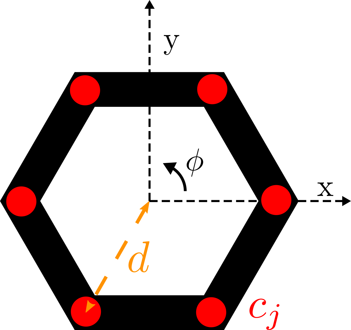
Figure 2: Illustration of some key quantities for the robot. The six red dots corresponding to the corners of the plate are used as our CBFs by deriving the forward kinematics of each point. The quantity $d$ represents the distance to these corners, $\phi$ represents the angle of rotation for the vector pointing to each corner from the center.

Our barrier functions will then take the form,

$$b_{j}(q)=c_{j}(q)-\epsilon_{j},$$ (14)

where $\epsilon_{j}>0$ is a parameter to specify the distance from contact that the safety constraint should be enforced. This is a function of relative degree two. Indeed, most functions based on the kinematics of robots with dynamics of the form (11) will be relative degree two. Therefore, to get the remaining quantities that are necessary for the CBF, we must find the Jacobian of these functions and the time derivatives of those Jacobians. The Jacobians are simply

$$J_{j}(q)=\frac{\partial c_{j}(q)}{\partial q}.$$ (15)

We omit inclusion of the explicit solution of the Jacobians due to their length, but they are easily calculated using a symbolic computing package. The time derivatives of the Jacobians, $\dot{J}_{j}$, are similarly calculated. We can then form matrices by stacking the safety constraints and their Jacobians, $b(q)=[b_{1},...,b_{N}]^{T}$, $J(q)=[J_{1},...,J_{N}]^{T}$, $\dot{J}(q)=[\dot{J}_{1},...,\dot{J}_{N}]^{T}$, where $N$ is the number of constraints. Note that $b$, $J$, and $\dot{J}$ all have limits that are well defined as $\theta\rightarrow 0$ (straight configuration). Finally, by choosing both class $\mathcal{K}$ functions (the relative degree of the safety constraint is two) in (3) as linear functions with constant coefficient $p>0$, the HOCBF constraints corresponding to (5) are

$$L_{f}^{2}b+L_{g}L_{f}bu+2pL_{f}b+p^{2}b\geq 0,$$ (16)

where $u=\tau$, $f=[\dot{q},M^{-1}(C\dot{q}+G+K+D\dot{q})]$ and $g=[0,M^{-1}]$ corresponding to the dynamics (11). Specifically, by substituting $\dot{b}=L_{f}b=J\dot{q}$, $\ddot{b}=L_{f}^{2}b+L_{g}L_{f}bu=J\ddot{q}+\dot{J}\dot{q}$ into (16), we have the following HOCBF constraints:

$$p^{2}b+2pJ\dot{q}+JM^{-1}(-C\dot{q}-G-Kq-D\dot{q}+\tau)+\dot{J}\dot{q}>0,$$ (17)

where dependencies on $q$ have been omitted for readability. The above inequality constraint can be included in the optimization as follows,

$$\min_{\tau} \frac{1}{2}||\tau-\tau_{\mathrm{nom}}||^{2}$$ (18)

s.t. Safety (HOCBF) Constraint (17).

We use the time-discretization method mentioned at the end of Sec. II-A to solve the above optimization, and it is reduced to a sequence of QPs in the form of (7).

IV Simulation Results

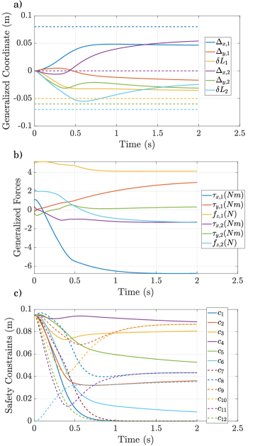
Figure 3: Results in Simulation. a) Shows the generalized coordinates and set points for a two segment simulated soft-rigid manipulator. b) Output torques from QP (18). c) Safety constraint values during the simulation. Note that there are 6 functions per segment for a total of 12.

We implement the previously discussed safety constraints in a simulation to control the dynamics (11) for a two link soft-rigid hybrid manipulator. The simulator is written in Julia and we compute the mass and coriolis matrices using Featherstone’s algorithms [22]. Elasticity and damping are taken to be linear. We forward integrate the closed loop system using the DifferentialEquations package [23], and we solve QP (18) using the Convex package [24]. For both packages, the default solvers proved to be adequate for our needs.

Parameters are set to $L_{0}=0.1\mathrm{m}$, $d=0.04\mathrm{m}$, $r=0.05\mathrm{m}$, bending stiffness $\kappa_{\theta}=10\mathrm{\frac{Nm}{rad}}$, axial stiffness $\kappa_{L}=10\mathrm{\frac{N}{m}}$, bending damping $\beta_{\theta}=5\mathrm{\frac{Nms}{rad}}$, axial damping $\beta_{L}=5\mathrm{\frac{Ns}{m}}$, and module mass $m_{j}=0.15\mathrm{kg}$. PD gains are set to $K_{\mathrm{P}}=5$ and $K_{\mathrm{P}}=1$ and $\epsilon_{j}=0.005\mathrm{m}$ for all barrier functions. We simulate from initial conditions $(q,\dot{q})=(\mathbf{0},\mathbf{0})$ and attempt to reach a set point $\overline{q}=[0.08,0.0,-0.05,0.0,-0.06,-0.07]^{T}$.

Results are shown in Fig. 3. We note that, as is evident from the plots, the desired set point is not possible without moving through the contact. This can be seen by observing Fig. 3c, where safety constraint function reach zero, but are kept from crossing the boundary due to the invariant property of CBFs.

V Hardware Results

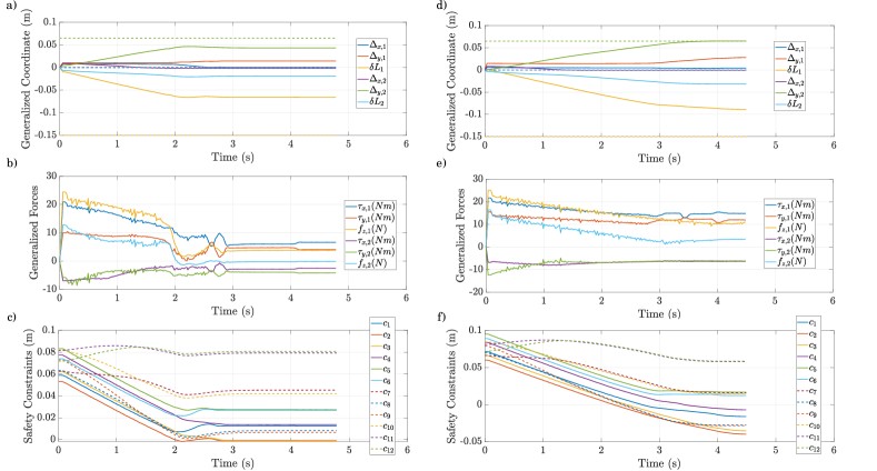
Figure 4: Plots for experiments on hardware. a) Generalized coordinates and set points for two segment manipulator controlled with a CBF. b) Commanded generalized forces from Eq. (18). c) Safety constraint values during an experiment. Note that there are 6 functions per segment for a total of 12. Note that the barrier functions are prevented from dropping below zero. d) Generalized coordinates and set points for two segment manipulator controlled with PD+. e) Commanded generalized forces from Eq. (12). f) Safety constraints (which are not actually enforced by the nominal controller and thus are allowed to be violated).

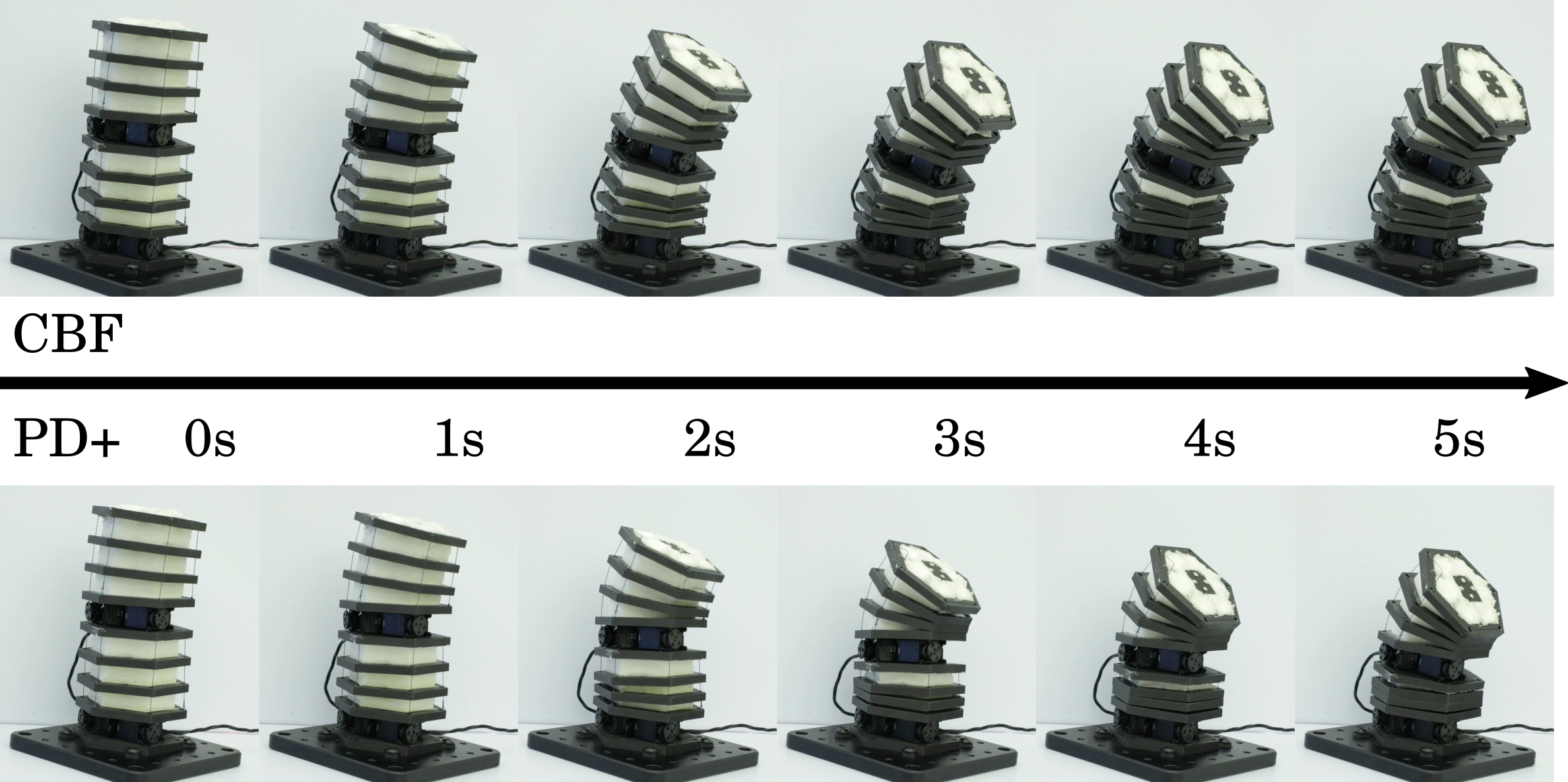
Figure 5: Top: snapshots from trials controlled by QP (18). Bottom: snapshots from PD+ controlled trial

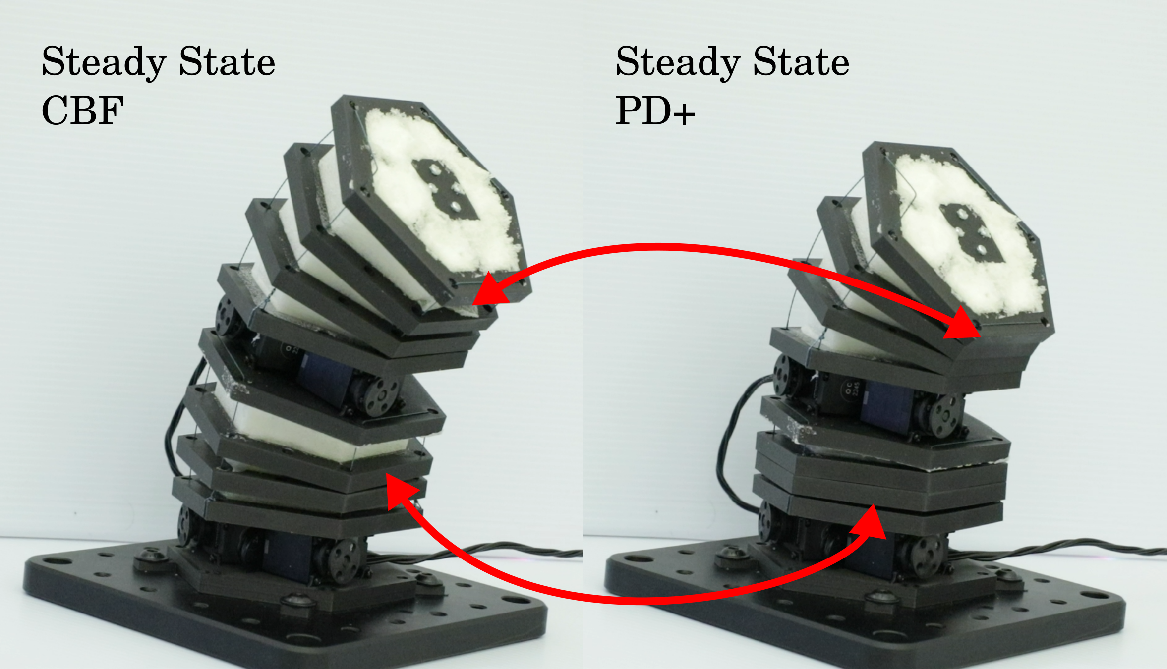
Figure 6: Zoomed in images from the end of the two experiments of Fig. 5 to highlight the physical difference in convergence.

We use the hardware shown in Fig. 1 to validate our approach. The hardware consists of Dynamixel servo motors that actuate cables to bend and compress the PCC segments. We interface with the Dynamixels via the serial port in a Python script. To speed up the code, we calculate the mass matrix, Coriolis matrix, Jacobians, and Jacobian time derivatives using a C program that is called from Python. The QP is solved using the Python CVXPY module [25, 26]. Finally, the decision variables output by our QP are generalized forces acting on our state variables and need to be transformed such that they take the form of cable tensions. We do this using the transformation from [20], along with another simple transformation to account for the fact that we have three cables.

To identify the parameters of our hardware, we measure those that are readily measurable (mass, geometric properties), measure stiffness using simple feedforward experiments, and use a least squares method to identify damping and (linear) actuator gain parameters as in [7, 27]. For our barrier functions, $\epsilon_{j}=0.005\mathrm{m}$ for all safety constraints.

Our code runs at a variable rate from $33$ to $50\mathrm{Hz}$. We begin at rest and attempt to reach a set point $\overline{q}=[0.0,0.0,-0.15,0.0,-0.065,0.0]^{T}$, which is significantly beyond the barrier for both modules. Results are shown in Fig. 4. We can see that the barrier functions are able to successfully prevent the system from crossing the barrier functions when CBFs are used, whereas the standard PD+ controller obviously attempts to reach the set point. This also results in a roughly 50% difference in actuator output at steady state, as can be observed from comparing Fig. 4b and e. We also show snapshots of this behavior in Fig. 5. The last snapshots from each are enlarged in Fig. 6, and it is evident that the case using our CBF method is able to attenuate the controller at (or in this case before) the contact, whereas the PD+ controller obviously does not have this capability.

VI Discussion

We have shown that incorporating a CBF into a strategy for controlling serial soft-rigid hybrid robots is an effective strategy for regulating self contact. This result is easily extended to task space by utilizing Khatib’s transformations [28, 7] and reformulating the cost function by mapping the generalized torques to operational space.

One open issue with this work is that, in the common case where the robot is cylindrical, it is not clear how to specify the barrier function points. One can attempt to write the barrier function as the forward kinematics of a point on the perimeter, but the Hessian of this function, which is used to calculate the time derivative, contains a singularity at $\theta=0$ (straight). It is an open question how to deal with this, and it will likely be important in the much broader context where it is necessary to calculate signed distance functions for points on a soft robot perimeter.

A potential issue with this control approach is that it essentially sacrifices the nice stability property of the nominal controller when the CBF is active. The common way to deal with this is to incorporate a CLF as well, but these competing constraints may be in conflict, resulting in an infeasible QP. [29] provides an interesting solution to this problem using a passivity constraint, which would be interesting to implement in future work.

In conclusion, we demonstrated a Control Barrier Function workflow for regulating self contact for serial soft-rigid hybrid systems. We derived barrier functions of second degree for a Piecewise Constant Curvature system and used them in a QP based framework for effective control both in simulation and on hardware.

References

- [1] J. M. Bern, F. Zargarbashi, A. Zhang, J. Hughes, and D. Rus, “Simulation and Fabrication of Soft Robots with Embedded Skeletons,” in 2022 International Conference on Robotics and Automation (ICRA), May 2022, pp. 5205–5211.
- [2] W. Zhu, C. Lu, Q. Zheng, Z. Fang, H. Che, K. Tang, M. Zhu, S. Liu, and Z. Wang, “A Soft-Rigid Hybrid Gripper With Lateral Compliance and Dexterous In-Hand Manipulation,” IEEE/ASME Transactions on Mechatronics, vol. 28, no. 1, pp. 104–115, Feb. 2023.
- [3] E. Coevoet, Y. Adagolodjo, M. Lin, C. Duriez, and F. Ficuciello, “Planning of Soft-Rigid Hybrid Arms in Contact With Compliant Environment: Application to the Transrectal Biopsy of the Prostate,” IEEE Robotics and Automation Letters, vol. 7, no. 2, pp. 4853–4860, Apr. 2022.
- [4] J. Zhang, T. Wang, J. Wang, M. Y. Wang, B. Li, J. X. Zhang, and J. Hong, “Geometric Confined Pneumatic Soft–Rigid Hybrid Actuators,” Soft Robotics, vol. 7, no. 5, pp. 574–582, Oct. 2020.
- [5] C. Della Santina, C. Duriez, and D. Rus, “Model-Based Control of Soft Robots: A Survey of the State of the Art and Open Challenges,” IEEE Control Systems Magazine, vol. 43, no. 3, pp. 30–65, Jun. 2023.
- [6] Z. J. Patterson, A. P. Sabelhaus, and C. Majidi, “Robust Control of a Multi-Axis Shape Memory Alloy-Driven Soft Manipulator,” IEEE Robotics and Automation Letters, vol. 7, no. 2, pp. 2210–2217, Apr. 2022.
- [7] C. Della Santina, R. K. Katzschmann, A. Bicchi, and D. Rus, “Model-based dynamic feedback control of a planar soft robot: Trajectory tracking and interaction with the environment,” The International Journal of Robotics Research, vol. 39, no. 4, pp. 490–513, Mar. 2020.
- [8] C. Della Santina, M. Bianchi, G. Grioli, F. Angelini, M. Catalano, M. Garabini, and A. Bicchi, “Controlling Soft Robots: Balancing Feedback and Feedforward Elements,” IEEE Robotics & Automation Magazine, vol. 24, no. 3, pp. 75–83, Sep. 2017.
- [9] K. P. Tee, S. S. Ge, and E. H. Tay, “Barrier lyapunov functions for the control of output-constrained nonlinear systems,” Automatica, vol. 45, no. 4, pp. 918–927, 2009.
- [10] P. Wieland and F. Allgower, “Constructive safety using control barrier functions,” in Proc. of 7th IFAC Symposium on Nonlinear Control System, 2007.
- [11] S. P. Boyd and L. Vandenberghe, Convex optimization. New York: Cambridge university press, 2004.
- [12] A. D. Ames, J. W. Grizzle, and P. Tabuada, “Control barrier function based quadratic programs with application to adaptive cruise control,” in Proc. of 53rd IEEE Conference on Decision and Control, 2014, pp. 6271–6278.
- [13] P. Glotfelter, J. Cortes, and M. Egerstedt, “Nonsmooth barrier functions with applications to multi-robot systems,” IEEE control systems letters, vol. 1, no. 2, pp. 310–315, 2017.
- [14] W. Xiao and C. Belta, “Control barrier functions for systems with high relative degree,” in Proc. of 58th IEEE Conference on Decision and Control, Nice, France, 2019, pp. 474–479.
- [15] C. Khazoom, D. Gonzalez-Diaz, Y. Ding, and S. Kim, “Humanoid Self-Collision Avoidance Using Whole-Body Control with Control Barrier Functions,” in 2022 IEEE-RAS 21st International Conference on Humanoid Robots (Humanoids), Nov. 2022, pp. 558–565.
- [16] H. K. Khalil, Nonlinear Systems. Prentice Hall, third edition, 2002.
- [17] W. Xiao, C. G. Cassandras, and C. Belta, Safe Autonomy with Control Barrier Functions: Theory and Applications. Springer Nature, 2023.
- [18] J. M. Bern, L. Z. Yañez, E. Sologuren, and D. Rus, “Contact-Rich Soft-Rigid Robots Inspired by Push Puppets,” in 2022 IEEE 5th International Conference on Soft Robotics (RoboSoft), Apr. 2022, pp. 607–613.
- [19] R. J. Webster and B. A. Jones, “Design and Kinematic Modeling of Constant Curvature Continuum Robots: A Review,” The International Journal of Robotics Research, vol. 29, no. 13, pp. 1661–1683, Nov. 2010.
- [20] C. Della Santina, A. Bicchi, and D. Rus, “On an Improved State Parametrization for Soft Robots With Piecewise Constant Curvature and Its Use in Model Based Control,” IEEE Robotics and Automation Letters, vol. 5, no. 2, pp. 1001–1008, Apr. 2020.
- [21] C. Della Santina, R. K. Katzschmann, A. Bicchi, and D. Rus, “Model-based dynamic feedback control of a planar soft robot: Trajectory tracking and interaction with the environment,” The International Journal of Robotics Research, vol. 39, no. 4, pp. 490–513, Mar. 2020.
- [22] R. Featherstone, Rigid body dynamics algorithms. Springer, 2014.
- [23] C. Rackauckas and Q. Nie, “DifferentialEquations.jl–a performant and feature-rich ecosystem for solving differential equations in Julia,” Journal of Open Research Software, vol. 5, no. 1, 2017.
- [24] M. Udell, K. Mohan, D. Zeng, J. Hong, S. Diamond, and S. Boyd, “Convex optimization in Julia,” SC14 Workshop on High Performance Technical Computing in Dynamic Languages, 2014.
- [25] S. Diamond and S. Boyd, “CVXPY: A Python-embedded modeling language for convex optimization,” Journal of Machine Learning Research, vol. 17, no. 83, pp. 1–5, 2016.
- [26] A. Agrawal, R. Verschueren, S. Diamond, and S. Boyd, “A rewriting system for convex optimization problems,” Journal of Control and Decision, vol. 5, no. 1, pp. 42–60, 2018.
- [27] L. Ljung, “System identification,” in Signal Analysis and Prediction. Springer, 1998, pp. 163–173.
- [28] O. Khatib, “A unified approach for motion and force control of robot manipulators: The operational space formulation,” IEEE Journal on Robotics and Automation, vol. 3, no. 1, pp. 43–53, Feb. 1987.
- [29] V. Kurtz, P. M. Wensing, and H. Lin, “Control Barrier Functions for Singularity Avoidance in Passivity-Based Manipulator Control,” in 2021 60th IEEE Conference on Decision and Control (CDC), Dec. 2021, pp. 6125–6130.