ONE-LOOP CORRECTION CONTRIBUTIONS IN THE DECOUPLING LIMIT OF GENERALIZED YUKAWA MODEL

Abstract

In this paper we consider generalized Yukawa model, which consists of two Dirac fermions and two scalar fields. One of the scalar bosons in this model is assumed to be much heavier than the other particles, so it decouples at low energies. Low-energy effective Lagrangian (EL) of this model is derived. This Lagrangian describes contributions of the heavy scalar in observables. We consider cross-sections of $s$- and $t$-channel processes, obtained within the complete model and its low-energy approximation. Contributions of one-loop corrections in these cross-sections coming from light particles of the model are analyzed. These are corrections to the parameters of the heavy boson and contributions of one-loop mixing of light and heavy scalars. We identify ranges of the model Yukawa couplings where these corrections are significant. We get that if interaction between fermions and either light or heavy scalar is strong enough, then the derived EL could not be applied for description of the analyzed processes cross-sections even when heavy scalar decouples. Implications of present results for searches of new particles beyond the Standard model are considered.

Keywords: low-energy effective Lagrangian, decoupling, generalized Yukawa model, one-loop corrections, new physics searches

1 Introduction

There exist many models of physics beyond the Standard model (SM), which introduce new heavy particles. Signals of such new states could be parametrized either within a complete model of new physics or its low-energy approximation. The latter consists of effective Lagrangian (EL), which describes the effects of interactions with heavy particles on the dynamics of light fields when heavy states decouple. Parameters of this EL should be constrained by an experimental data analysis. These constraints, in turn, are translated into some limits to the parameters of the corresponding complete model. This approach is employed in many researches [2, 5]. It is often assumed that the loop corrections to parameters of a heavy particle coming from the light and the heavy sectors of a corresponding UV-complete model are negligible small in the decoupling limit.

Contrary to this statement, we show in this paper that in the latter case the radiative corrections given by light fields are considerable for some values of model parameters.

Our research is conducted for two scattering processes, which occur either in $s$- or $t$-channels only. These processes are $\psi_{1}\bar{\psi}_{1}\rightarrow\psi_{2}\bar{\psi}_{2}$ and $\psi_{1}\psi_{2}\rightarrow\psi_{1}\psi_{2}$. Transformational properties of fields and complex interactions within the SM are inessential for our analyzis. Hence, we consider generalized Yukawa model. It consists of scalars $\phi$ and $\chi$ and fermions $\psi_{1}$ and $\psi_{2}$. We put $\chi$ boson to be much heavier than the other particles of the model, so it decouples at low energies. We derive low-energy EL for this model. This EL approximates tree-level contribution of $\chi$ boson in observables when $\chi$ decouples. We work out cross-sections of the considered reactions within complete and effective models. Contributions of radiative corrections in these cross-sections are analyzed. These are corrections to the $\chi$ boson parameters and contributions of one-loop mixing of light and heavy scalars. We identify ranges of the model Yukawa couplings where radiative corrections are significant. We find out that if it is so, then the tree-level EL could not be applied to describe cross-sections of the reactions at low energies.

The low-energy EL of the considered model contains only four-fermion contact vertexes besides the Lagrangian of light fields. Hence, our research is relevant for scattering processes which are contributed only by four-fermion interaction vertexes within an EFT treatment.

This paper is organized as follows. In section 2 we introduce our model and derive the low-energy EL of it. In sections 3 and 4 we analyze contributions of loop corrections in the $s$- and $t$-channel processes cross-sections, respectively. Finally, we conclude our analyzis and discuss its results in section 5.

2 The model

Let us consider the generalized Yukawa model. This model consists of two Dirac fermions $\psi_{1}$ and $\psi_{2}$ and two scalar bosons $\phi$ and $\chi$. Fermions and scalars of the model interact via Yukawa’s couplings. We assume that $\chi$ is much heavier than the other particles. The Lagrangian of the model reads:

$$\mathcal{L}=\frac{1}{2}\left(\partial_{\mu}\phi\right)^{2}-\frac{1}{2}\mu^{2}\phi^{2}+\frac{1}{2}\left(\partial_{\mu}\chi\right)^{2}-\frac{1}{2}\Lambda^{2}\chi^{2}-\lambda\phi^{4}-\rho\phi^{2}\chi^{2}-\xi\chi^{4}+\sum\limits_{a=1;2}\bar{\psi}_{a}\left(i\hat{\partial}-m_{a}-g_{\phi}\phi-g_{\chi}\chi\right)\psi_{a}.$$ (1)

Here $\mu$ and $\Lambda$ are masses of scalars $\phi$ and $\chi$, while $m_{1}$ and $m_{2}$ are masses of fermions $\psi_{1}$ and $\psi_{2}$, respectively. $\lambda$, $\rho$ and $\xi$ denote scalar self-interaction constants. $g_{\phi}$ and $g_{\chi}$ are Yukawa couplings. All parameters of the model are real.

$\chi$ decouples at the energies of particles which are much less than $\Lambda$. In the model proposed here $\Lambda\gg\mu;\,m_{1};\,m_{2}$, so interactions of $\phi$, $\psi_{1}$ and $\psi_{2}$ could be described with a low-energy effective Lagrangian (EL) at such energies. To derive this EL, we integrate out $\chi$ bosons in the initial and final states of the model fields:

$$\exp\left(i\int d^{4}x\mathcal{L}_{eff}\right)=\int\mathcal{D}\chi\exp\left(i\int d^{4}x\mathcal{L}\right)=\int\mathcal{D}\chi e^{iS}.$$ (2)

We calculate this functional integral in the Gaussian approximation, similarly to [3]. In this approximation action $S$ is expanded into a Taylor series around some given $\chi_{0}(x)$:

$$S=S[\chi_{0}]+\int d^{4}x\frac{\delta S}{\delta\chi(x)}\Bigr{|}_{\chi=\chi_{0}}(\chi-\chi_{0})(x)+\frac{1}{2}\int d^{4}x_{1}d^{4}x_{2}\frac{\delta^{2}S}{\delta\chi(x_{1})\delta\chi(x_{2})}(\chi-\chi_{0})(x_{1})(\chi-\chi_{0})(x_{2})+O\left[(\chi-\chi_{0})^{3}\right].$$ (3)

Then we put $\chi_{0}(x)$ such that $\frac{\delta S}{\delta\chi(x)}\Bigr{|}_{\chi=\chi_{0}}=0$. Thus, $\chi_{0}(x)$ satisfies classical motion equation for $\chi$. Terms $O\left[(\chi-\chi_{0})^{3}\right]$ in (3) are all proportional to scalar self-interaction couplings. We assume that these constants are so small that terms $O\left[(\chi-\chi_{0})^{3}\right]$ could be neglected. Finally, $S$ is approximated with the following expression:

$$S\approx S[\chi_{0}]+\frac{1}{2}\int d^{4}x_{1}d^{4}x_{2}\frac{\delta^{2}S}{\delta\chi(x_{1})\delta\chi(x_{2})}(\chi-\chi_{0})(x_{1})(\chi-\chi_{0})(x_{2}).$$ (4)

Equation for $\chi_{0}(x)$ reads:

$$(\partial^{2}+\Lambda^{2})\chi_{0}=-2\rho\phi^{2}\chi_{0}-4\xi\chi_{0}^{3}-J_{\chi},\quad J_{\chi}=g_{\chi}\sum\limits_{a=1;2}\bar{\psi}_{a}\psi_{a}.$$ (5)

We solve this equation employing the same approximations as in [3, 7]. That is, we represent $\chi_{0}(x)$ as a series in growing powers of couplings:

$$\chi_{0}=\chi_{0}^{(0)}+\chi_{0}^{(1)}+\chi_{0}^{(2)}+...\Rightarrow\begin{cases}(\partial^{2}+\Lambda^{2})\chi_{0}^{(0)}=-J_{\chi}\\ (\partial^{2}+\Lambda^{2})\chi_{0}^{(1)}=-2\rho\phi^{2}\chi_{0}^{(0)}-4\xi\left(\chi_{0}^{(0)}\right)^{3}\\ ...\end{cases}.$$

In the decoupling region we neglect the derivative term in (5), since $|\partial^{2}\chi|\ll\Lambda^{2}|\chi|$. Hence, $\chi_{0}(x)$ approximately reads:

$$\chi_{0}\approx\chi_{0}^{(0)}=-\frac{1}{\Lambda^{2}}J_{\chi}.$$ (6)

Here we have omitted the other terms in the expansion for $\chi_{0}(x)$, since they are suppressed by higher powers of $\Lambda^{-2}$. We derive EL for our model only up to terms $O(\Lambda^{-4})$.

We put (6) to the expression for action $S$ and get the first term in (4):

$$S[\chi_{0}]=\int d^{4}x\left[\frac{1}{2}\left(\partial_{\mu}\phi\right)^{2}-\frac{1}{2}\mu^{2}\phi^{2}-\lambda\phi^{4}+\sum\limits_{a=1;2}\bar{\psi}_{a}(i\hat{\partial}-m_{a}-g_{\phi}\phi)\psi_{a}+\frac{1}{2\Lambda^{2}}J_{\chi}^{2}\right].$$ (7)

For the second term in (4) we have:

$$\frac{\delta^{2}S}{\delta\chi(x_{1})\delta\chi(x_{2})}\Bigr{|}_{\chi=\chi_{0}}=-\left[\partial^{2}+\Lambda^{2}+2\rho\phi^{2}(x_{1})\right]\delta(x_{1}-x_{2}).$$

We put this expression to (2) and integrate over the fluctuations $(\chi-\chi_{0})(x)$. Eventually, we omit infinite constants and get the following expression for $\mathcal{L}_{eff}$:

$$i\int d^{4}x\mathcal{L}_{eff}=iS[\chi_{0}]-\frac{1}{2}{\rm Tr}\ln{\left(\partial^{2}+\Lambda^{2}+2\rho\phi^{2}\right)}.$$

The second term here could be expanded in powers of $\rho$:

$${\rm Tr}\ln{\left(\partial^{2}+\Lambda^{2}+2\rho\phi^{2}\right)}={\rm Tr}\ln{(\partial^{2}+\Lambda^{2})}+2\rho\int d^{4}x(\partial^{2}+\Lambda^{2})^{-1}(x;x)\phi^{2}(x)+O(\rho^{2}).$$

The first term here is constant so we omit it. The second term implements radiative correction to the $\phi$ mass from the $\chi$ loop. This correction is absorbed in the renormalized $\phi$ mass. The other terms could be neglected, since they are suppressed either by higher powers of $\rho$ or $\Lambda^{-2}$.

Finally, we get the following expression for $\mathcal{L}_{eff}$:

$$\mathcal{L}_{eff}=\frac{1}{2}\left(\partial_{\mu}\phi\right)^{2}-\frac{1}{2}\mu^{2}\phi^{2}-\lambda\phi^{4}+\sum\limits_{a=1;2}\bar{\psi}_{a}(i\hat{\partial}-m_{a}-g_{\phi}\phi)\psi_{a}+\frac{g_{\chi}^{2}}{2\Lambda^{2}}\left(\bar{\psi}_{1}\psi_{1}+\bar{\psi}_{2}\psi_{2}\right)^{2}.$$ (8)

The last term here corresponds to non-renormalizable contact four-fermion interactions. This term is suppressed by $\Lambda^{-2}$, so when $\Lambda\rightarrow\infty$ these contact interactions vanish.

Values of the parameters $m_{1}$, $m_{2}$ and $\mu$ are fixed in our analyzis. These values are shown in table 1.

Table 1: Values of the model parameters which are fixed in the analyzis

$m_{1}$	$m_{2}$	$\mu$
$0.511\,MeV$	$105.658\,MeV$	$5\,GeV$

3 The $s$-channel scattering process

Let us consider the scattering process $\psi_{1}\bar{\psi}_{1}\rightarrow\psi_{2}\bar{\psi}_{2}$, which takes place in $s$-channel only. The diagram of this process is shown in Fig. 1. We derive matrix element of this process in the improved Born approximation. The latter implies that all one-loop radiative corrections are taken into account except for box diagrams. It was shown in [4] that contribution of box diagrams in the considered $s$-process cross-section within the model (1) is less than $1\,\%$ of the contribution of one-particle-reducible diagrams. Thus, we omit boxes in our treatment.

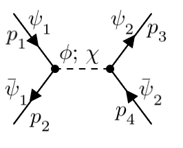
FIG. 1: Diagram of the reaction $\psi_{1}\bar{\psi}_{1}\rightarrow\psi_{2}\bar{\psi}_{2}$ within the UV-complete model described by the Lagrangian (1)

Cross-section of this reaction within the UV-complete model (1) in the center-of-mass reference frame reads:

$$\sigma(\psi_{1}\bar{\psi}_{1}\rightarrow\psi_{2}\bar{\psi}_{2})=\Phi^{(s)}(s)\left|\begin{pmatrix}-ig_{\phi}\Gamma_{\phi}(s;m_{2})\\ -ig_{\chi}\Gamma_{\chi}(s;m_{2})\end{pmatrix}^{T}\begin{pmatrix}s-\mu^{2}-\Pi_{\phi\phi}(s)&-\Pi_{\phi\chi}(s)\\ -\Pi_{\phi\chi}(s)&s-\Lambda^{2}-\Pi_{\chi\chi}(s)\end{pmatrix}^{-1}\begin{pmatrix}-ig_{\phi}\Gamma_{\phi}(s;m_{1})\\ -ig_{\chi}\Gamma_{\chi}(s;m_{1})\end{pmatrix}\right|^{2},$$ (9)

$$\Phi^{(s)}(s)=\frac{s}{16\pi}\left(1-\frac{4m_{2}^{2}}{s}\right)^{\frac{3}{2}}\sqrt{1-\frac{4m_{1}^{2}}{s}},\quad s=(p_{1}+p_{2})^{2},\quad\Gamma_{\phi;\chi}(s;m_{12})=1+\delta\Gamma_{\phi;\chi}^{(\phi)}(s;m_{12})+\delta\Gamma_{\phi;\chi}^{(\chi)}(s;m_{12}).$$ (10)

Hereafter all cross-sections are averaged over polarizations of initial fermions and summed over polarizations of fermions in a final state. Quantities $\delta\Gamma_{\phi}^{(\phi)}(s;m_{12})$, $\delta\Gamma_{\phi}^{(\chi)}(s;m_{12})$ and $\delta\Gamma_{\chi}^{(\phi)}(s;m_{12})$, $\delta\Gamma_{\chi}^{(\chi)}(s;m_{12})$ in (9) denote radiative corrections to Yukawa interaction with $\phi$ and $\chi$, respectively. Second argument of these functions is a mass of the fermionic field involved in the corresponding vertex. Diagrams of these corrections are displayed in Fig. 2.

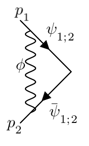
(a) $\delta\Gamma_{\phi;\chi}^{(\phi)}(s;m_{12})$

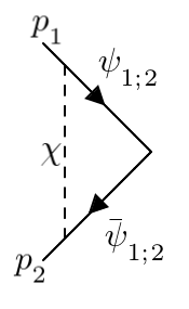
(b) $\delta\Gamma_{\phi;\chi}^{(\chi)}(s;m_{12})$

FIG. 2: Diagrams of loop corrections to Yukawa vertexes in the model

We impose the following renormalization conditions on $\Gamma_{\phi}(s;m_{12})$ and $\Gamma_{\chi}(s;m_{12})$:

$$\Gamma_{\phi}(\mu^{2};m_{12})=1,\quad\Gamma_{\chi}(\Lambda^{2};m_{12})=1.$$ (11)

Corrections $\delta\Gamma_{\phi;\chi}^{(\phi)}(s;m_{12})$ and $\delta\Gamma_{\phi;\chi}^{(\chi)}(s;m_{12})$ are calculated numerically with LoopTools software [8]. Function $\Phi^{(s)}(s)$ in (9) is a kinematical factor. It is introduced by integration over the momentum space of final particles and by summation over polarization states of initial and final particles.

$\Pi_{\phi\phi}(s)$, $\Pi_{\phi\chi}(s)$ and $\Pi_{\chi\chi}(s)$ in (9) denote radiative corrections in propagators of scalar fields. They are contributed by the diagrams shown in Fig. 3.

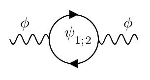
(a) $\Pi_{\phi\phi}(s)$

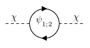
(b) $\Pi_{\chi\chi}(s)$

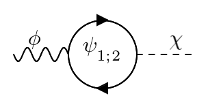
(c) $\Pi_{\phi\chi}(s)$

FIG. 3: Radiative corrections in the two-point Green functions of scalar fields

$\Pi_{\phi\phi}(s)$ and $\Pi_{\chi\chi}(s)$ describe loop corrections to the masses of $\phi$ and $\chi$ bosons, accordingly. $\Pi_{\phi\chi}(s)$ corresponds to one-loop mixing of $\phi$ and $\chi$. We calculate these corrections analytically and impose the following renormalization conditions on them:

$$\text{Re}\,\Pi_{\phi\phi}(\mu^{2}) =0,\quad\text{Re}\,\Pi_{\chi\chi}(\Lambda^{2})=0,\quad\text{Re}\,\Pi_{\phi\chi}(\kappa^{2})=0,$$

$$\frac{\partial\text{Re}\,\Pi_{\phi\phi}(s)}{\partial s}\Bigr{|}_{s=\mu^{2}} =0,\quad\frac{\partial\text{Re}\,\Pi_{\chi\chi}(s)}{\partial s}\Bigr{|}_{s=\Lambda^{2}}=0,\quad\frac{\partial\text{Re}\,\Pi_{\phi\chi}(s)}{\partial s}\Bigr{|}_{s=\kappa^{2}}=0.$$ (12)

Here $\kappa^{2}$ is an arbitrary renormalization scale. We put $\kappa=1\,GeV$. One-loop contributions from scalar self-interactions in $\Pi_{\phi\phi}(s)$ and $\Pi_{\chi\chi}(s)$ are absorbed by renormalized masses of $\phi$ and $\chi$.

Example graph of $\sigma(s)$ dependency on the center-of-mass energy $\sqrt{s}$ is shown in Fig. 4.

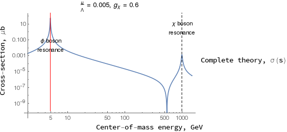
FIG. 4: $\sigma$ as a function of the center-of-mass energy of $\psi_{1}$ and $\bar{\psi}_{1}$. Hereafter red solid line and black dashed line in the plots mark values of masses of $\phi$ and $\chi$ bosons, respectively

As could be seen in Fig. 4, $\sigma(s)$ develops two maximums, which correspond to the masses of $\phi$ and $\chi$. Dip between these maximums is introduced by interference of $\phi$ and $\chi$ exchange amplitudes in the expression of $\sigma(s)$ and one-loop mixing of the two fields.

We derive approximate expression for (9) in the limit $\Lambda^{2}\gg s$. If $\chi$ boson is very heavy, then we neglect its loop corrections to Yukawa vertexes, so the diagram in Fig. 2(b) is omitted and $\lim\limits_{s\ll\Lambda^{2}}\delta\Gamma_{\phi;\chi}^{(\chi)}(s;m_{12})\rightarrow 0$. $\sigma(s)$ in the limit of large $\Lambda$ reads:

$$\sigma(\psi_{1}\bar{\psi}_{1}\rightarrow\psi_{2}\bar{\psi}_{2})\Bigr{|}_{\Lambda^{2}\gg s} \approx\Phi^{(s)}(s)\left|\frac{(-ig_{\phi})^{2}\Gamma_{\phi}^{(eff)}(s;m_{2})\Gamma_{\phi}^{(eff)}(s;m_{1})}{s-\mu^{2}-\Pi_{\phi\phi}(s)}+\delta\mathcal{M}^{(mix)}(s)+\delta\mathcal{M}^{(4-ferm)}(s)\right|^{2}=\sigma_{approx}(s),$$ (13)

$$\Gamma_{\phi;\chi}^{(eff)}(s;m_{12}) =1+\delta\Gamma_{\phi;\chi}^{(\phi)}(s;m_{12}),\quad\delta\mathcal{M}^{(4-ferm)}(s)=\frac{g_{\chi}^{2}\Gamma_{\chi}^{(eff)}(s;m_{1})\Gamma_{\chi}^{(eff)}(s;m_{2})}{\Lambda^{2}+\Pi_{\chi\chi}(s)},$$

$$\delta\mathcal{M}^{(mix)}(s) =\frac{2g_{\phi}g_{\chi}\Pi_{\phi\chi}(s)}{\left(\Lambda^{2}+\Pi_{\chi\chi}(s)\right)\left(s-\mu^{2}-\Pi_{\phi\phi}(s)\right)}.$$

Here we omitted terms of higher orders in Yukawa couplings. There are three terms in the squared modulus factor in (13). The first one corresponds to the s-channel reaction involving only light particles of the model. The second term $\delta\mathcal{M}^{(mix)}(s)$ is proportional to $\Pi_{\phi\chi}(s)$ and it describes contribution of one-loop mixing of scalar fields in $\sigma(s)$. Finally, the third term $\delta\mathcal{M}^{(4-ferm)}$ corresponds to the four-fermion interaction in the low-energy EFT. Unlike four-fermion vertex in (8), $\delta\mathcal{M}^{(4-ferm)}(s)$ contains polarization operator of $\chi$ boson $\Pi_{\chi\chi}(s)$. Since $\Pi_{\chi\chi}(s)\sim g_{\chi}^{2}$, $|\Pi_{\chi\chi}(s)|$ is significant if $|g_{\chi}|$ is big. Loop corrections to the Yukawa vertexes of $\chi$ boson also enter $\delta\mathcal{M}^{(4-ferm)}(s)$ in functions $\Gamma_{\chi}^{(eff)}(s;m_{1})$ and $\Gamma_{\chi}^{(eff)}(s;m_{2})$. These corrections emerge only from loops of light boson $\phi$ and their contributions are proportional to $g_{\phi}^{2}$. Hence, we should take them into account if interactions within light sector of the model are powerful enough.

Now we turn to the cross-section of the process $\psi_{1}\bar{\psi}_{1}\rightarrow\psi_{2}\bar{\psi}_{2}$ within the effective theory (8). Diagrams which are taken into account in this case are shown in Fig. 5.

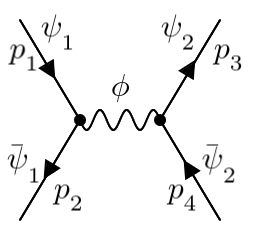
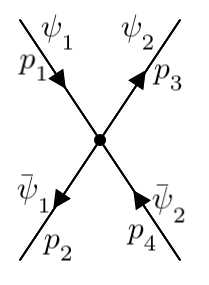
FIG. 5: Diagrams which contribute cross-section of the reaction in the low-energy effective theory

Left diagram in Fig. 5 emerges from interactions of light fields only. We derive matrix element of this diagram in the improved Born approximation. Right diagram in Fig. 5 corresponds to the four-fermion contact interaction, which is specific to the low-energy EL (8). Cross-section of the reaction $\psi_{1}\bar{\psi}_{1}\rightarrow\psi_{2}\bar{\psi}_{2}$ within the low-energy effective theory is as follows:

$$\sigma_{eff}(\psi_{1}\bar{\psi}_{1}\rightarrow \psi_{2}\bar{\psi}_{2})=\Phi^{(s)}(s)\left|\frac{(-ig_{\phi})^{2}\Gamma_{\phi}^{(eff)}(s;m_{1})\Gamma_{\phi}^{(eff)}(s;m_{2})}{s-\mu^{2}-\Pi_{\phi\phi}(s)}+\frac{g_{\chi}^{2}}{\Lambda^{2}}\right|^{2}.$$ (14)

Here we also take into account term $g_{\chi}^{4}\Lambda^{-4}$ despite the assumptions used in section 2. This term ensures that $\sigma_{eff}(s)\geq 0$. It could be observed that, contrary to (13), radiative corrections to $g_{\chi}$ and $\Lambda$, as well as contribution of bosons one-loop mixing, are absent in (14).

Example of $\sigma_{eff}(s)$ dependency on the center-of-mass energy $\sqrt{s}$ is shown in Fig. 6. Similarly to $\sigma(s)$, $\sigma_{eff}(s)$ develops a maximum which corresponds to the mass of light $\phi$ boson. There is also a dip in $\sigma_{eff}(s)$ at $s>\mu^{2}$, which is introduced by interference between amplitudes of two diagrams in Fig. 5.

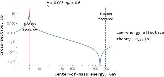
FIG. 6: $\sigma_{eff}$ as a function of the center-of-mass energy of $\psi_{1}$ and $\bar{\psi}_{1}$

We plot $\sigma(s)$, $\sigma_{approx}(s)$ and $\sigma_{eff}(s)$ at different values of $\Lambda$, $g_{\phi}$ and $g_{\chi}$ as functions of $\sqrt{s}$ in Fig. 7. We also plot contribution of polarization operator of $\chi$ boson, contribution of radiative corrections to Yukawa vertexes of the latter and relative contribution of the one-loop mixing term in $\sigma_{approx}(s)$ in Fig. 9. Magnitudes of the first two corrections are also shown in the plots in Fig. 8. We analyze magnitudes and contributions of various radiative corrections at low energies and describe regions in the model parameters space where they are significant.

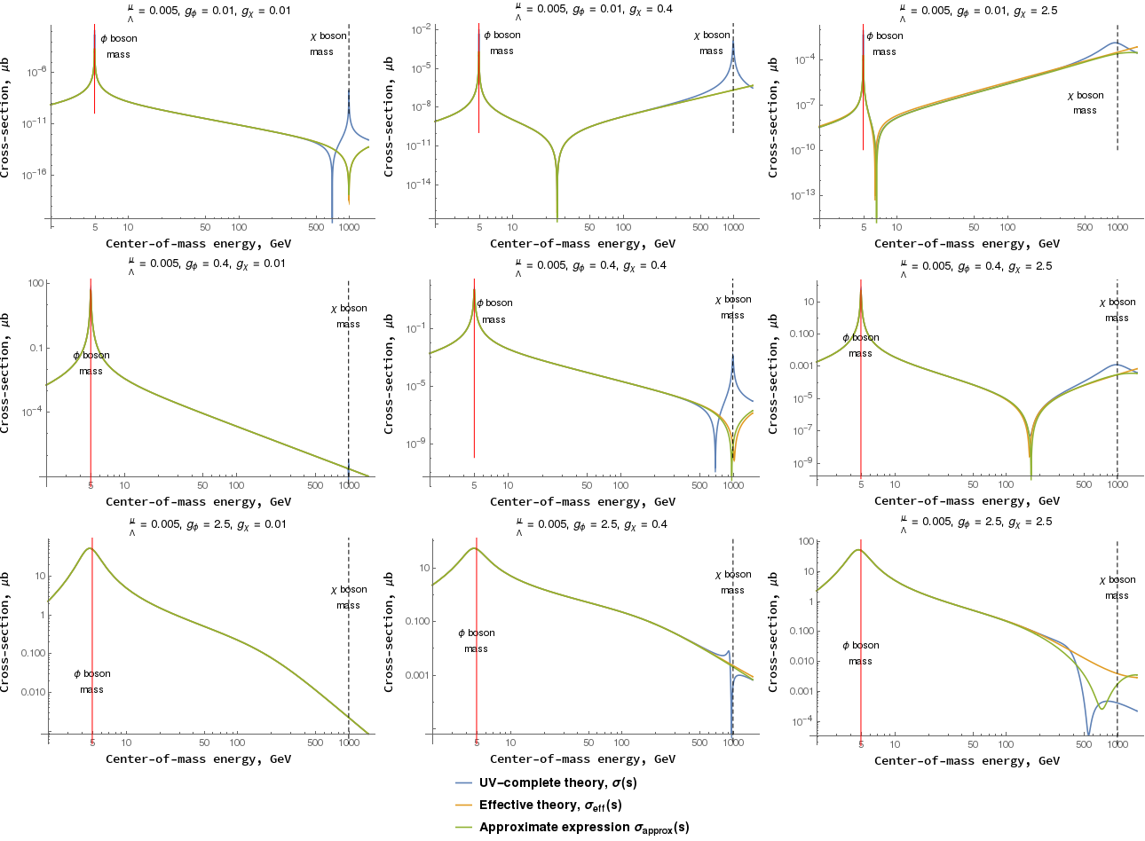
FIG. 7: $\sigma(s)$, $\sigma_{eff}(s)$ and $\sigma_{approx}(s)$ at $\Lambda=200\mu$ and different values of $g_{\phi}$ and $g_{\chi}$, $s$-channel process

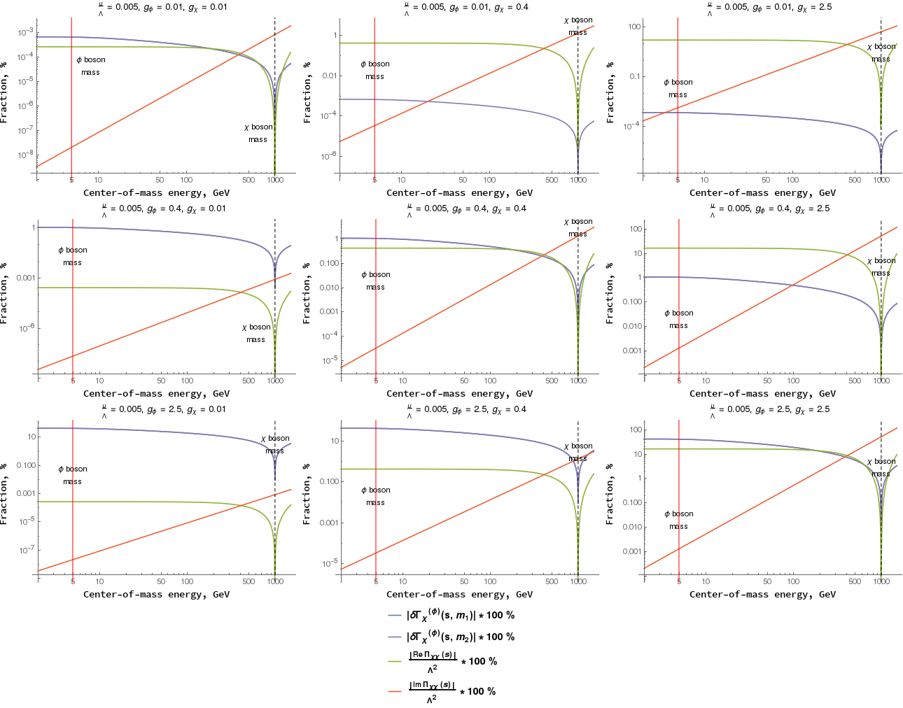
FIG. 8: Values of loop corrections relative to corresponding parameters of the model at $\Lambda=200\mu$ and different values of $g_{\phi}$ and $g_{\chi}$, $s$-channel process

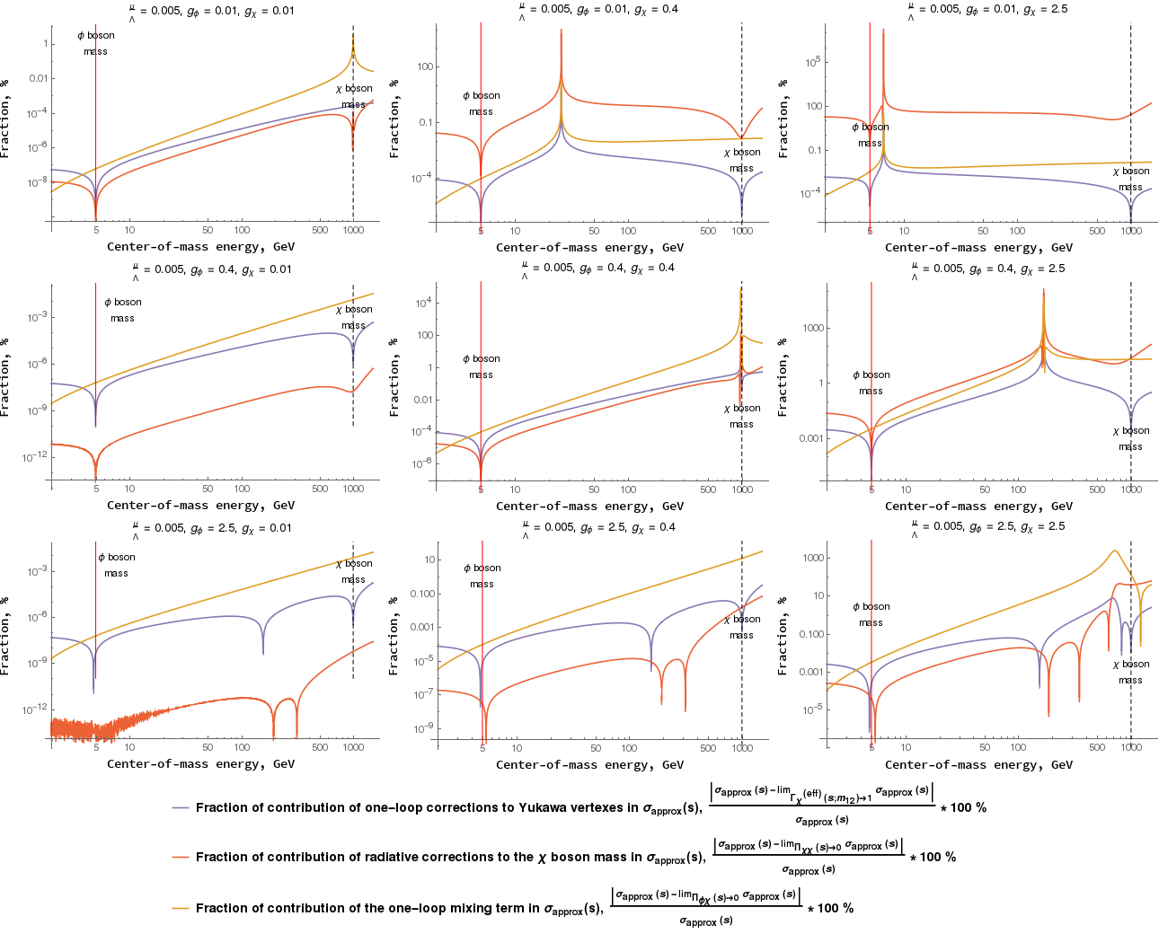
FIG. 9: Contributions of loop corrections to Yukawa vertexes and mass of $\chi$ boson and one-loop mixing contribution in $\sigma_{approx}(s)$ at $\Lambda=200\mu$ and different values of $g_{\phi}$ and $g_{\chi}$, $s$-channel process

We begin with the scenario when both $|g_{\phi}|$ and $|g_{\chi}|$ are small. If it is so, then $\Pi_{\chi\chi}(s)$ and one-loop mixing of scalar fields could be neglected in the reaction cross-section within the low-energy EFT, while $\Gamma_{\chi}^{(eff)}(s;m_{12})$ could be considered equal to $1$. In the model studied in this paper we have that $|\delta\Gamma_{\chi}^{(\phi)}(s;m_{12})|\lesssim 0.01$, $|\text{Re}\,\Pi_{\chi\chi}(s)|\lesssim 0.01\Lambda^{2}$ and $|\text{Im}\,\Pi_{\chi\chi}(s)|\lesssim 0.01\Lambda^{2}$ if $|g_{\phi}|<0.4$ and $|g_{\chi}|<0.4$. These radiative corrections and one-loop mixing term contribute less than $1\,\%$ in $\sigma_{approx}(s)$ at $s\ll\Lambda^{2}$ for $20\mu\leq\Lambda\leq 200\mu$. Hence, if couplings of the model fermions to light and heavy scalars are small, then (8) is applicable for the description of the reaction cross-section at low energies.

Now we proceed to the scenarios when loop corrections in $\sigma(s)$ are significant and should be taken into account at low energies.

It could be observed in the top right plot in Fig. 9 that if $|g_{\chi}|$ is big, then contribution of radiative correction to $\Lambda$ in $\sigma_{approx}(s)$ is significant. For $|g_{\phi}|\approx 0.01$ and $2.5\leq|g_{\chi}|\leq 3$ $\Pi_{\chi\chi}(s)$ contributes more than $10\,\%$ of $\sigma_{approx}(s)$ even at $s=O(\mu^{2})$. In this limit all the other loop corrections are negligible, since they are proportional to $g_{\phi}^{2}$. $|\Pi_{\chi\chi}(s)|\gtrsim 0.1\Lambda^{2}$ for almost the whole range of energies $2m_{2}<\sqrt{s}\leq\Lambda$ at $g_{\phi}\in[0.01;\,0.05]$ and $g_{\chi}\in[2.5;\,3]$ for a wide range of $\Lambda$ variation. Real and imaginary parts of $\Pi_{\chi\chi}(s)$ become dominant at low and high energies, respectively. We find out that for $0.01\leq|g_{\phi}|\leq 0.05$ and $2.5\leq|g_{\chi}|\leq 3$ at low energies $\sqrt{s}\lesssim 0.5\Lambda$ $|\text{Re}\,\Pi_{\chi\chi}(s)|>|\text{Im}\,\Pi_{\chi\chi}(s)|$ and at higher energies $\sqrt{s}\gtrsim 0.5\Lambda$ $|\text{Im}\,\Pi_{\chi\chi}(s)|$ dominates over $|\text{Re}\,\Pi_{\chi\chi}(s)|$. If $|g_{\phi}|\ll|g_{\chi}|$ and $|g_{\chi}|$ is big, then contribution of heavy scalar in $\sigma(s)$ within the UV-complete theory (1) is significantly suppressed by $\Pi_{\chi\chi}(s)$. Consequently, it is considerably overestimated in $\sigma_{eff}(s)$. According to the cross-sections plots in Fig. 7, $\sigma_{eff}(s)$ provides under- or overestimation of $\sigma(s)$ at different $s$. Hence, in the considered limit of couplings values and at $s=O(\mu^{2})$ loop corrections to $\chi$ boson mass should be taken into account in the process cross-section at low energies.

Contributions of loop corrections to Yukawa vertexes and one-loop mixing term in the process cross-section are small in the limit when $|g_{\phi}|\ll|g_{\chi}|$ and Yukawa couplings of $\chi$ are big. It follows from the top right plot in Fig. 9 that if $g_{\phi}\in[0.01;\,0.05]$ and $g_{\chi}\in[2.5;\,3]$, then both contributions consist less than $1\,\%$ of $\sigma_{approx}(s)$ for most values of energies in the range $4m_{2}^{2}<s\leq\Lambda^{2}$. According to the top right plot in Fig. 8, $|\delta\Gamma_{\chi}^{(\phi)}(s;m_{12})|<10^{-3}$ for such values of $g_{\phi}$. We also recognize that difference between $\sigma_{eff}(s)$ and $\sigma(s)$ at $s\ll\Lambda^{2}$ decreases for higher values of $\Lambda$ in the discussed limit of couplings magnitudes. This phenomenon is described by the Appelquist-Carazzone decoupling theorem.

If $|g_{\phi}|$ is not small, then one-loop mixing term in $\sigma_{approx}(s)$ is significant with respect to the four-fermion interaction contribution there. Relation of these two terms absolute values is as follows:

$$\frac{|\delta\mathcal{M}^{(mix)}(s)|}{|\delta\mathcal{M}^{(4-ferm)}(s)|}=\frac{2g_{\phi}^{2}|P(s)|}{\left|\left[s-\mu^{2}-\Pi_{\phi\phi}(s)\right]\Gamma_{\chi}^{(eff)}(s;m_{1})\Gamma_{\chi}^{(eff)}(s;m_{2})\right|},\quad\Pi_{\phi\chi}(s)=g_{\phi}g_{\chi}P(s).$$

Here $P(s)$ does not depend on any Yukawa couplings. It could be seen from this expression that relation between $|\delta\mathcal{M}^{(mix)}(s)|$ and $|\delta\mathcal{M}^{(4-ferm)}(s)|$ does not depend on $g_{\chi}$ and is proportional to $g_{\phi}^{2}$. $|\delta\mathcal{M}^{(mix)}(s)|$ consists significant fraction of $|\delta\mathcal{M}^{(4-ferm)}(s)|$ near $s=\mu^{2}$ or if $|g_{\phi}|$ is big. For the model discussed here we have that $\left|\delta\mathcal{M}^{(mix)}(s)\right|\gtrsim 0.5\left|\delta\mathcal{M}^{(4-ferm)}(s)\right|$ for $\mu^{2}<s\leq\Lambda^{2}$, $20\mu\leq\Lambda\leq 200\mu$ if $|g_{\phi}|\gtrsim 1$. Hence, if Yukawa coupling between light boson and fermions is strong enough, then one-loop mixing of scalars should not be ignored in the process cross-section in the decoupling limit.

Since one-loop corrections in $\Gamma_{\chi}^{(eff)}(s;m_{12})$ are proportional to $g_{\phi}^{2}$, then they also should be taken into account if $|g_{\phi}|$ is big. In our model we have that $|\delta\Gamma_{\chi}^{(\phi)}(s;m_{12})|\gtrsim 0.1$ if $|g_{\phi}|>1$.

4 The $t$-channel scattering process

We now consider a process $\psi_{1}\psi_{2}\rightarrow\psi_{1}\psi_{2}$, which takes place in $t$-channel only. Feynman diagram of this process is displayed in Fig. 10.

FIG. 10: Diagram of the reaction $\psi_{1}\psi_{2}\rightarrow\psi_{1}\psi_{2}$ within the UV-complete model described by the Lagrangian (1)

Cross-section of this reaction within the UV-complete theory in the improved Born approximation is as follows:

$$\frac{d\sigma(\psi_{1}\psi_{2}\rightarrow\psi_{1}\psi_{2})}{d\Omega}=\Phi^{(t)}(t)\left|\begin{pmatrix}-ig_{\phi}\Gamma_{\phi}(t;m_{2})\\ -ig_{\chi}\Gamma_{\chi}(t;m_{2})\end{pmatrix}^{T}\begin{pmatrix}t-\mu^{2}-\Pi_{\phi\phi}(t)&-\Pi_{\phi\chi}(t)\\ -\Pi_{\phi\chi}(t)&t-\Lambda^{2}-\Pi_{\chi\chi}(t)\end{pmatrix}^{-1}\begin{pmatrix}-ig_{\phi}\Gamma_{\phi}(t;m_{1})\\ -ig_{\chi}\Gamma_{\chi}(t;m_{1})\end{pmatrix}\right|^{2},$$ (15)

$$\Phi^{(t)}(t)=\frac{(4m_{1}^{2}-t)(4m_{2}^{2}-t)}{64\pi^{2}(E_{1}+E_{2})^{2}},\quad t=(p_{1}-p_{3})^{2}=2\left(m_{1}^{2}-E_{1}E_{3}+|\overline{p}_{1}||\overline{p}_{3}|\cos{\theta}\right)=(p_{2}-p_{4})^{2},$$

$$d\Omega=2\pi\sin{\theta}d\theta,\quad E_{1}=\sqrt{\overline{p}_{1}^{2}+m_{1}^{2}},\quad E_{2}=\sqrt{\overline{p}_{2}^{2}+m_{2}^{2}},\quad E_{3}=\sqrt{\overline{p}_{3}^{2}+m_{1}^{2}}.$$

We omit box diagrams from our treatment of the $t$-channel process, too. It is assumed that their contributions are negligible, as it is for the $s$-process considered in section 3.

Expression (15) is also derived in the initial particles center-of-mass reference frame. Functions $\Gamma_{\phi}(t;m_{12})$ and $\Gamma_{\chi}(t;m_{12})$ represent Yukawa vertexes of $\phi$ and $\chi$ bosons with one-loop corrections. Diagrams of the latter are displayed in Fig. 2. Function $\Phi^{(t)}(t)$ in (15) is a kinematical factor. It is introduced by partial integration over the momentum space of final particles and summation over polarization states of initial and final particles.

As it could be seen from the expression (15), matrix element of the $t$-channel process has similar analytical structure as that of the $s$-channel process. That is, squared modulus factors in (9) and (15) are analytically similar and depend on Mandelstam invariants $s$ and $t$, accordingly. The same holds for the cross-section of this reaction $d\sigma_{eff}(\psi_{1}\psi_{2}\rightarrow\psi_{1}\psi_{2})/d\Omega$ within the low-energy EFT (8) and approximate expression of the cross-section $d\sigma_{approx}(\psi_{1}\psi_{2}\rightarrow\psi_{1}\psi_{2})/d\Omega$ derived from (15) in the limit $|t|\ll\Lambda^{2}$. Hence, we do not provide expressions for $d\sigma_{eff}(\psi_{1}\psi_{2}\rightarrow\psi_{1}\psi_{2})/d\Omega$ and $d\sigma_{approx}(\psi_{1}\psi_{2}\rightarrow\psi_{1}\psi_{2})/d\Omega$ in this section. Examples of the $t$-channel process cross-sections are shown in Fig. 11.

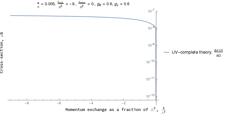
(a) UV-complete theory

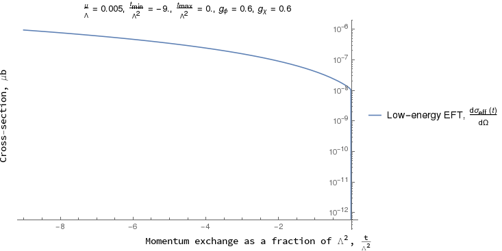
(b) Low-energy EFT

FIG. 11: Example cross-sections of the process $\psi_{1}\psi_{2}\rightarrow\psi_{1}\psi_{2}$

We conduct the same analyzis for the scattering process $\psi_{1}\psi_{2}\rightarrow\psi_{1}\psi_{2}$ as it was carried out for the process $\psi_{1}\bar{\psi}_{1}\rightarrow\psi_{2}\bar{\psi}_{2}$ in section 3. Corresponding plots are shown in Fig. 12, 13 and 14.

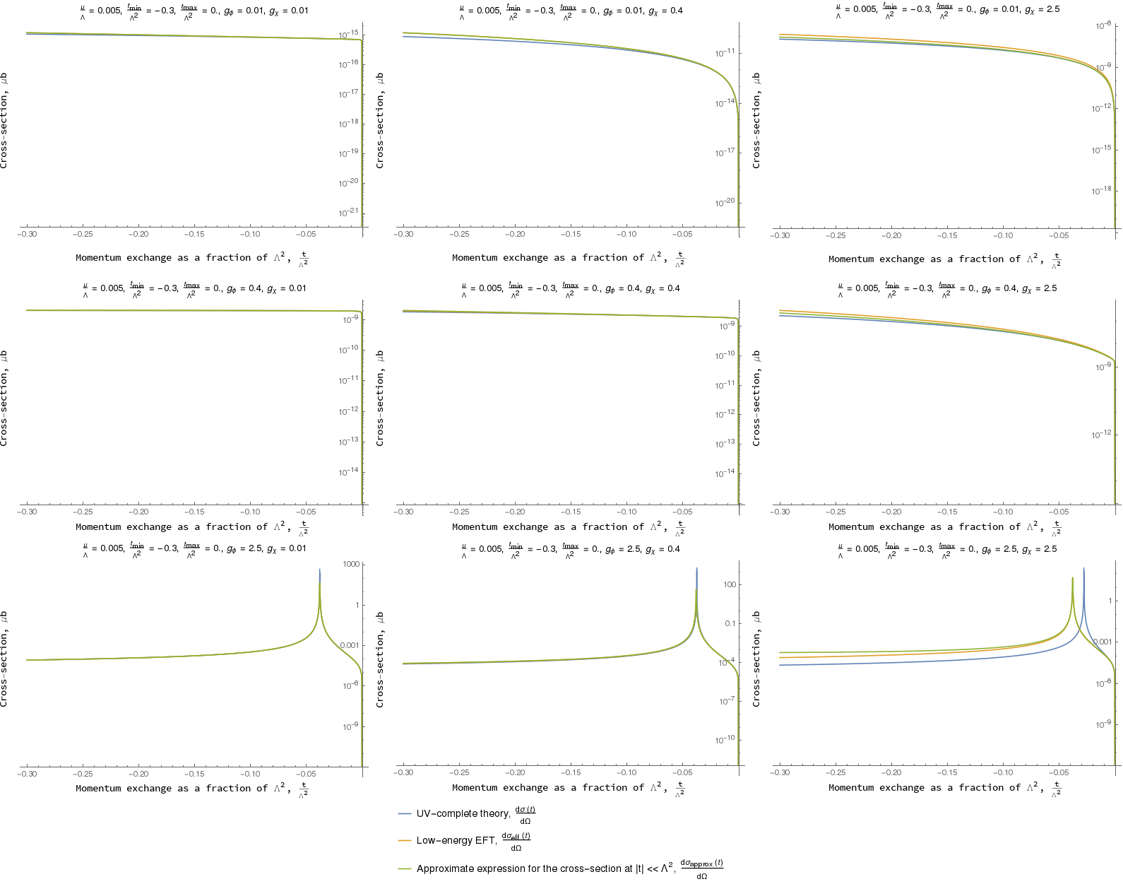
FIG. 12: $\frac{d\sigma(t)}{d\Omega}$, $\frac{d\sigma_{eff}(t)}{d\Omega}$ and $\frac{d\sigma_{approx}(t)}{d\Omega}$ at $\Lambda=200\mu$, $t$-channel process

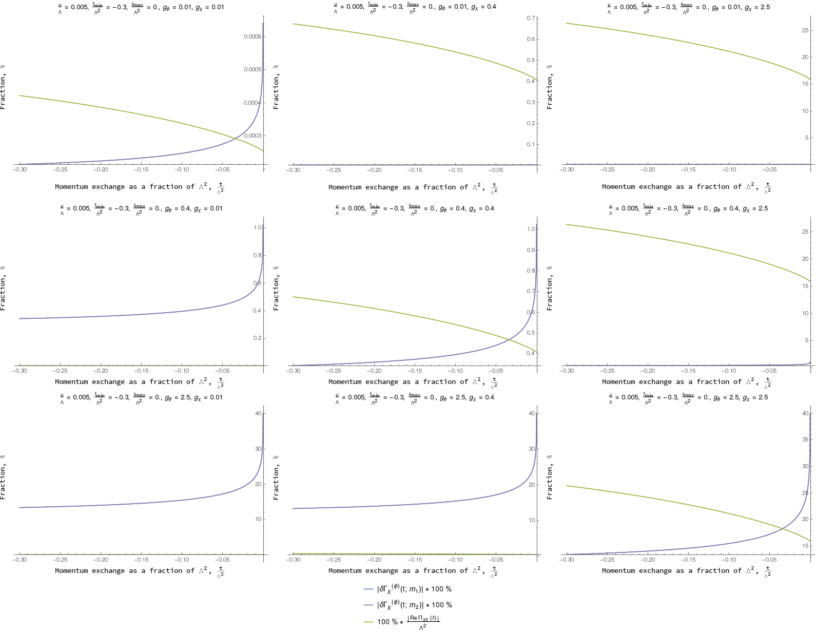
FIG. 13: Magnitudes of loop corrections to Yukawa vertexes and mass of $\chi$ boson, $t$-channel process

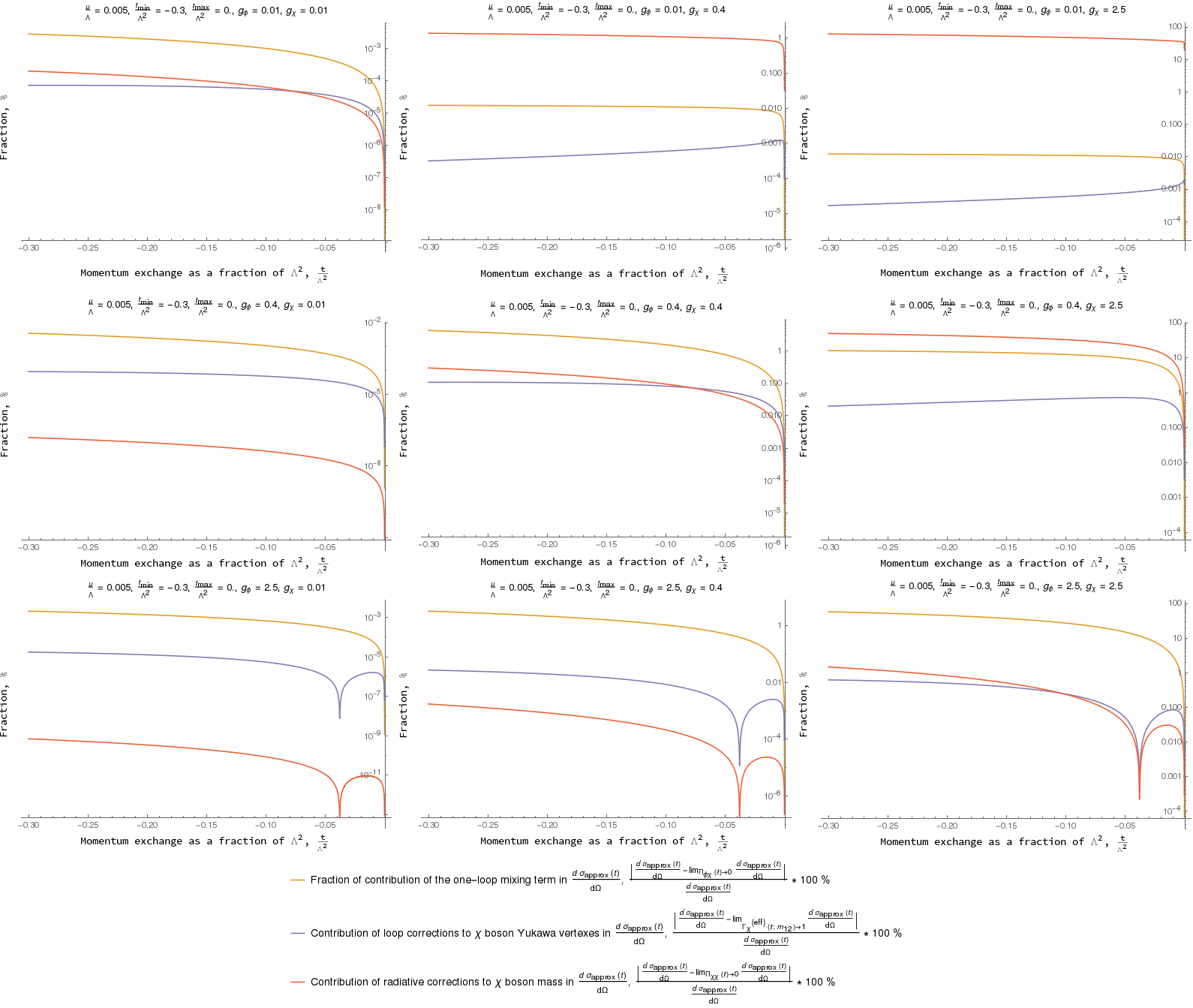
FIG. 14: Relative contributions of various loop corrections in $\frac{d\sigma_{approx}(t)}{dt}$, $t$-channel process

Similarly to section 3, we first identify a scenario when radiative corrections to couplings and mass of $\chi$ boson, as well as one-loop mixing contribution, are negligible at $|t|\ll\Lambda^{2}$. It could be seen in the graphs in Fig. 13 that it is so if both $|g_{\phi}|$ and $|g_{\chi}|$ are small. In our model we have that if $|g_{\phi}|\lesssim 0.4$ and $|g_{\chi}|\lesssim 0.4$, then $|\text{Re}\,\Pi_{\chi\chi}(t)|<0.05\Lambda^{2}$ and $|\delta\Gamma_{\chi}^{(\phi)}(t;m_{12})|<0.05$ for $-1.5\Lambda^{2}\leq t<0$ and $20\mu\leq\Lambda\leq 200\mu$. $\delta\mathcal{M}^{(mix)}$ is also small – $|\delta\mathcal{M}^{(mix)}|<0.15|\delta\mathcal{M}^{(4-ferm)}|$ in the same ranges of $t$ and $\Lambda$. All these corrections contribute less than $6\,\%$ of $d\sigma_{approx}/d\Omega$ for $-0.3\Lambda^{2}\leq t<0$ and $20\mu\leq\Lambda\leq 200\mu$. This could be observed in Fig. 14 for $\Lambda=200\mu$.

Now we proceed to scenarios when radiative corrections are considerable.

If $|g_{\chi}|$ is big, then $|\Pi_{\chi\chi}(t)|$ is significant with respect to $\Lambda^{2}$. In our model we have that $|\Pi_{\chi\chi}(t)|\gtrsim 0.1\Lambda^{2}$ at $|t|\ll\Lambda^{2}$ if $2\leq|g_{\chi}|\leq 3$. According to plots in Fig. 14, this correction contributes more than $10\,\%$ of $d\sigma_{approx}(t)/d\Omega$ for $-0.3\Lambda^{2}\leq t<0$ if $0.01\leq|g_{\phi}|\leq 0.05$ – in this limit all other corrections are negligible. This takes place for $20\mu\leq\Lambda\leq 200\mu$. Thus, for such choice of the model parameters loop correction to heavy boson mass becomes significant even at low $|t|$.

If $|g_{\phi}|$ is big, then loop corrections to $\chi$ boson Yukawa vertexes are considerable. In present model we have that if $|g_{\phi}|\gtrsim 1.5$ then $|\delta\Gamma_{\chi}^{(\phi)}(t;m_{12})|\geq 0.1$ at $|t|\ll\Lambda^{2}$. This is so for $20\mu\leq\Lambda\leq 200\mu$. The one-loop mixing term is also significant in the discussed limit. Namely, we have that $|\delta\mathcal{M}^{(mix)}|\geq 0.1|\delta\mathcal{M}^{(4-ferm)}|$ if $|g_{\phi}|\geq 0.8$ and $|t|\ll\Lambda^{2}$. If $|g_{\phi}|$ is very big, then $|\delta\mathcal{M}^{(mix)}|>|\delta\mathcal{M}^{(4-ferm)}|$ even at small $|t|$. We find out that it is so if $|g_{\phi}|\geq 1.5$ and $100\mu\leq\Lambda\leq 200\mu$. If $\Lambda=20\mu$, then $|\delta\mathcal{M}^{(mix)}|$ is bigger than $|\delta\mathcal{M}^{(4-ferm)}|$ at small $|t|$ if $|g_{\phi}|\geq 2$. Thus, if interaction between light fermions and boson in the model is strong enough, then absolute values of contributions of both one-loop mixing and four-fermion interaction terms in the process cross-section might be numerically close to each other even at low $|t|$.

It could be observed in the cross-sections plots in Fig. 12 that if $|g_{\phi}|$ is big, then $d\sigma(t)/d\Omega$ develops a peak at some $t=t_{0}$. This peak corresponds to the point where determinant of the matrix in (15) is zero and $d\sigma(t)/d\Omega$ apparently diverges. That is, $t_{0}$ satisfies the following equation:

$$\left[t_{0}-\mu^{2}-\Pi_{\phi\phi}(t_{0})\right]\left[t_{0}-\Lambda^{2}-\Pi_{\chi\chi}(t_{0})\right]-\Pi_{\phi\chi}^{2}(t_{0})=0.$$

This equation contains terms of the fourth order in Yukawa couplings. Two-loop radiative corrections enter perturbative expansions at this order, too. Hence, the behaviour of $d\sigma(t)/d\Omega$ near the point $t=t_{0}$ could be studied only when two-loop diagrams are taken into account in the expressions for $\Pi_{\phi\phi}(t)$, $\Pi_{\phi\chi}(t)$ and $\Pi_{\chi\chi}(t)$. Such analyzis is beyond the scope of this paper, so we omit it for now.

5 Discussion and conclusion

In this paper we derived the low-energy effective Lagrangian of generalized Yukawa model in the limit when the heaviest scalar field of the model decouples. There are two scalars in the model – $\phi$ and $\chi$, which are light and heavy, respectively.

We analyzed contributions of radiative corrections from loops with light particles in the cross-sections of scattering processes within the model in the limit when $\chi$ boson decouples. Two reactions were considered – $\psi_{1}\bar{\psi}_{1}\rightarrow\psi_{2}\bar{\psi}_{2}$ and $\psi_{1}\psi_{2}\rightarrow\psi_{1}\psi_{2}$. These processes take place in $s$- and $t$-channel, respectively. We identified values of the model parameters when radiative corrections are insignificant at low energies and effective Lagrangian (8) is valid.

We find out that if $|g_{\phi}|$ and $|g_{\chi}|$ are small the loop corrections are negligible and the EL (8) is applicable for description of scattering processes at low energies. For present model it is so if $|g_{\phi}|<0.4$ and $|g_{\chi}|<0.4$.

If $|g_{\chi}|$ is big, then loop corrections to $\chi$ boson mass are to be considerable even at low energies. In our model, we have that if $|g_{\chi}|>2.5$ then the corrections in Fig. 3(b) give more than $10\,\%$ of the $\chi$ boson mass. These corrections suppress the contribution of the heavy scalar in reaction cross-section. Hence, if $|g_{\chi}|$ is big, then (8) significantly overestimates $\chi$ boson contribution in the cross-sections when $\chi$ decouples.

If $|g_{\phi}|$ is not small, the contribution of the scalar field one-loop mixings is significant in either $s$- or $t$-channels. One-loop mixing of $\phi$ and $\chi$ is introduced by the diagram in Fig. 3(c). In our model, we get that if $|g_{\phi}|\gtrsim 1.5$, the contribution of one-loop mixing of scalars in the matrix elements of the considered reactions is bigger than $50\,\%$ of the four-fermion interaction term at $s\gtrsim\mu^{2}$ and $|t|\gtrsim\mu^{2}$ for $|g_{\chi}|<0.4$. Radiative corrections to Yukawa vertexes of $\chi$ boson are also significant in this limit, since they are proportional to $g_{\phi}^{2}$. These corrections are depicted in Fig. 2(a).

To conclude, in our research we have derived the conditions when radiative corrections are negligible in the decoupling limit in cross-sections of reactions within the generalized Yukawa model. According to these conditions, radiative corrections become significant if the interactions between light fermions and either light or decoupled scalar are not feeble. In such scenarios, expression (8) should not be used as the low-energy approximation of the model (1). The results obtained in this investigation could be applied to some models of new physics which extend the SM, such as the two-Higgs-doublet model (2HDM). The latter has a limit when new heavy particles decouple. So, low-energy EL could be derived for it [3]. Contributions of radiative corrections into cross-sections within the 2HDM should be estimated in the limit when heavy fields beyond the SM decouple. This is the problem left for the future.

References

[1]Brandt B. Loop corrections in a solvable UV-finite model and its effective field theory / F. T. Brandt, J. Frenkel, D. G. C. McKeon and G. S. S. Sakoda // Phys. Rev. D – 2023. – Vol. 107, 065008, arXiv:2302.11059v1 [hep-th], DOI: https://doi.org/10.1103/PhysRevD.107.065008
[2]CMS Collaboration Search for new physics using effective field theory in 13 TeV pp collision events that contain a top quark pair and a boosted Z or Higgs boson / CMS Collaboration // report number CMS-TOP-21-003, CERN-EP-2022-172, arXiv:2208.12837v1 [hep-ex], DOI: https://doi.org/10.48550/arXiv.2208.12837
[3]Dmytriiev M. Low-energy effective Lagrangian of the two-Higgs-doublet model / M. Dmytriiev, V. Skalozub // Journal of physics and electronics – 2021. – Vol. 29, No. 2, 8, arXiv:2206.07770v2 [hep-ph]
[4]Skalozub V. V. On direct search for dark matter in scattering processes within Yukawa model / V. V. Skalozub, M. S. Dmytriiev // Ukr. J. Phys. – 2021. – Vol. 66, No. 11, DOI:10.15407/ujpe66.11.936, arXiv:2007.06269v2
[5]Ellis J. Top, Higgs, Diboson and Electroweak Fit to the Standard Model Effective Field Theory / John Ellis, Maeve Madigan, Ken Mimasu, Veronica Sanz, Tevong You // JHEP – 2021. – 04, 279, DOI: 10.1007/JHEP04(2021)279
[6]Criado J. BSM Benchmarks for Effective Field Theories in Higgs and Electroweak Physics / D. Marzocca, F. Riva, J. Criado, S. Dawson, J. de Blas, B. Henning, D. Liu, C. Murphy, M. Perez-Victoria, J. Santiago, L. Vecchi, Lian-Tao Wang // report number LHC-HXSWG-2019-006, arXiv:2009.01249v1 [hep-ph], DOI: https://doi.org/10.48550/arXiv.2009.01249
[7]Bélusca-Maïto H. Higgs EFT for 2HDM and beyond / H. Bélusca-Maïto, A. Falkowski, D. Fontes, J. C. Romão, J. P. Silva // Eur. Phys. J. C – 2017. – 77, 3:176, DOI: 10.1140/epjc/s10052-017-4745-5
[8] T. Hahn, M. Perez-Victoria. Automatized one-loop calculations in 4 and D dimensions. Comput. Phys. Commun118, 153 (1999) 2-3. DOI: https://doi.org/10.1016/S0010-4655(98)00173-8.