Nonuniform Bose-Einstein condensate. II.
Doubly coherent states

We find stationary excited states of a one-dimensional system of $N$ spinless point bosons with repulsive interaction and zero boundary conditions by numerically solving the time-independent Gross-Pitaevskii equation. The solutions are compared with the exact ones found in the Bethe-ansatz approach. We show that the $j$th stationary excited state of a nonuniform condensate of atoms corresponds to a Bethe-ansatz solution with the quantum numbers $n_{1}=n_{2}=\ldots=n_{N}=j+1$. On the other hand, such $n_{1},\ldots,n_{N}$ correspond to a condensate of $N$ elementary excitations (in the present case the latter are the Bogoliubov quasiparticles with the quasimomentum $\hbar\pi j/L$, where $L$ is the system size). Thus, each stationary excited state of the condensate is “doubly coherent”, since it corresponds simultaneously to a condensate of $N$ atoms and a condensate of $N$ elementary excitations. We find the energy $E$ and the particle density profile $\rho(x)$ for such states. The possibility of experimental production of these states is also discussed.

1 Introduction

In the previous work [1], the ground state of a nonuniform condensate was studied. In the present work, we consider the stationary excited states of such a condensate. Excited states, which are solutions of the general time-dependent Gross-Pitaevskii (GP) equation, can be non-stationary (quasiparticles [2, 3, 4, 5, 6, 7, 8] and solitons [3, 7, 9, 10, 11, 12]) and stationary. The latter are solutions of a boundary value problem, being given by the stationary GP equation and boundary conditions (BCs). Such solutions can be of a vortex [2, 16, 17, 18, 19, 20, 21, 22, 23, 24] or a non-vortex type. Here we will consider the one-dimensional (1D) problem, where only non-vortex solutions are possible. Such solutions have been found for several systems [25, 26, 27, 28]. Seemingly, they were not observed experimentally.

Below we will find solutions for stationary excited states of a 1D system of spinless point bosons under zero BCs. Solutions for such a system have already been obtained and written in terms of the Jacobi elliptic functions [26]. We will find these solutions differently (numerically) and compare them with the exact ones obtained by the Bethe ansatz. Our main aim is to ascertain a relationship between the solutions of the GP equation and the elementary excitations of the system. To our knowledge, such an analysis has not been carried out before.

The structure of the paper is as follows. Section 2 contains the basic equations. The idea about the physical origin of stationary excited states of the condensate is formulated in section 3. In sections 4 and 5 we analyze solutions of the time-independent GP equation corresponding to a hole-like Lieb’s quasiparticle and an ideal crystal. In sections 6 and 7 we find a relationship between the solutions of the time-independent GP equation, exact solutions obtained in the Bethe-ansatz approach, and elementary quasiparticles. The final sections 8 and 9 are devoted to a discussion of the results obtained and possible experiments. In the Appendix we investigate whether the condensate $\Phi_{j_{0}}(x)$, which is a solution of the stationary GP equation, can be fragmented.

2 Initial equations

It is known that the substitution of the $c$-number ansatz

$$\hat{\Psi}(\mathbf{r},t)=\Psi(\mathbf{r},t)$$ (1)

into the Heisenberg equation results in the Gross-Pitaevskii equation [29, 30]

$$i\hbar\frac{\partial\Psi(\mathbf{r},t)}{\partial t}=-\frac{\hbar^{2}}{2m}\frac{\partial^{2}\Psi(\mathbf{r},t)}{\partial\mathbf{r}^{2}}+2c\Psi(\mathbf{r},t)|\Psi(\mathbf{r},t)|^{2}.$$ (2)

This equation describes a nonuniform condensate in a system of $N$ spinless bosons that interact through a point-like potential $U(|\mathbf{r}_{j}-\mathbf{r}_{l}|)=2c\delta(\mathbf{r}_{j}-\mathbf{r}_{l})$. In work [1] it was shown that if, instead of the $c$-number ansatz (1), we use a somewhat more accurate operator ansatz

$$\hat{\Psi}(\mathbf{r},t)=\hat{a}_{0}\Psi(\mathbf{r},t)/\sqrt{N},$$ (3)

then the Heisenberg equation leads to the equation

$$i\hbar\frac{\partial\Psi(\mathbf{r},t)}{\partial t}=-\frac{\hbar^{2}}{2m}\frac{\partial^{2}\Psi(\mathbf{r},t)}{\partial\mathbf{r}^{2}}+\left(1-\frac{1}{N}\right)2c\Psi(\mathbf{r},t)|\Psi(\mathbf{r},t)|^{2}.$$ (4)

This equation also follows from the ansatz

$$\Psi_{N}(\mathbf{r}_{1},\ldots,\mathbf{r}_{N},t)=\prod\limits_{j=1}^{N}[\Psi(\mathbf{r}_{j},t)/\sqrt{N}],$$ (5)

as was shown by the analysis of the $N$-particle Schrödinger equation [31] (see also [1]) and by a variational method [32]. Below, Eqs. (2) and (4) will be called the GP and GP_N equations, respectively. The GP_N equation differs from the GP one by the factor $\left(1-1/N\right)$. Ansätze (1), (3), and (5) are equivalent in the sense that each of them describes a system where all atoms are in the condensate $\Psi(\mathbf{r},t)$. Ansatz (1) is valid for $N\gg 1$, and ansätze (3) and (5) for $N\geq 2$.

In work [1] we studied the solutions of the stationary GP and GP_N equations, corresponding to the ground state of the condensate, for different values of $N$, the average particle density $\bar{\rho}=N/L$, and the coupling constant $\gamma=c/\bar{\rho}$. The analysis has shown that the GP_N equation describes the system in the near-free particle regime ($\gamma N^{2}\lesssim 1$) much more accurately than the GP equation does. This regime corresponds to small $N$ ($N\lesssim\gamma^{-1/2}$) or ultra-weak coupling ($\gamma\lesssim N^{-2}$). For weak coupling ($\gamma\lesssim 0.1$ and $N\gg 1$), the GP and GP_N equations describe the system with the same accuracy when $\gamma N^{2}\gg 1$.

In the present work, we consider a 1D system of $N$ spinless bosons with point repulsive interaction ($c>0$), which occupy the segment $[0,L]$ under zero BCs. We seek stationary solutions

$$\Psi(x,t)=e^{\epsilon t/i\hbar}\Phi(x),$$ (6)

so that the GP and GP_N equations take the forms

$$\epsilon\Phi(x)=-\frac{\hbar^{2}}{2m}\frac{\partial^{2}\Phi}{\partial x^{2}}+2c|\Phi|^{2}\Phi$$ (7)

and

$$\epsilon\Phi(x)=-\frac{\hbar^{2}}{2m}\frac{\partial^{2}\Phi}{\partial x^{2}}+\left(1-\frac{1}{N}\right)2c|\Phi|^{2}\Phi,$$ (8)

respectively, with the boundary conditions

$$\Phi(x=0)=\Phi(x=L)=0.$$ (9)

Let us find solutions of Eqs. (7) and (8) under BCs (9) which correspond to the excited states of the condensate. We will seek each solution in the form of an “elementary $j_{0}$-series” [1]

$$\Phi_{j_{0}}(x)=\sum\limits_{j=j_{0},3j_{0},5j_{0},\ldots}b_{j}\sqrt{2/L}\cdot\sin(k_{j}x),\quad k_{j}=\pi j/L.$$ (10)

The case $j_{0}=1$ corresponds to the ground state and was considered in [1]. Below we will find solutions for $j_{0}=2,3,\ldots,\infty$ by numerically solving Eqs. (7), (8) and (9) using the Newton method (for a description of this method, see work [1]). Since it is impossible to numerically find an infinite number of solutions ($j_{0}=2,3,\ldots,\infty$), we will limit ourselves to the cases $j_{0}=2,N$, which are of particular interest, and a few random $j_{0}$. According to our analysis, if the interaction is switched off ($\gamma=0$), the solutions transform into the solutions for a free particle in a box: $\Phi_{j_{0}}(x)|_{\gamma\rightarrow 0}\rightarrow b_{j_{0}}\sqrt{2/L}\,\sin(k_{j_{0}}x)$. To clarify the physical meaning of the solutions $\Phi_{j_{0}}(x)$ for $\gamma>0$, we will compare them with the exact solutions obtained by the Bethe ansatz.

In the GP and GP_N approaches, the condensate energy for the state $\Phi_{j_{0}}(x)$ is determined by the formula

$$E_{\mathrm{GP}}=\int\limits_{0}^{L}dx\left\{-\frac{\hbar^{2}}{2m}\Phi_{j_{0}}^{\ast}(x)\frac{\partial^{2}}{\partial x^{2}}\Phi_{j_{0}}(x)+qc|\Phi_{j_{0}}(x)|^{4}\right\},$$ (11)

where $q=1$ for the GP approach and $q=1-1/N$ for the GP_N one [1]. In the exact Bethe-ansatz approach, the energy of the system is

$$E_{\mathrm{Bethe}}=k_{1}^{2}+k_{2}^{2}+\ldots+k_{N}^{2},$$ (12)

where $|k_{j}|$ are solutions of the system of Gaudin’s equations [33, 34]

$$L|k_{p}|=\pi n_{p}+\sum\limits_{j=1}^{N}\left(\arctan{\frac{c}{|k_{p}|-|k_{j}|}}+\arctan{\frac{c}{|k_{p}|+|k_{j}|}}\right)|_{j\neq p},\quad p=1,\ldots,N.$$ (13)

Here the quantum numbers $n_{p}$ must be natural, i.e. $n_{p}=1,2,3,\ldots,\infty$ for each $p=1,2,\ldots,N$.

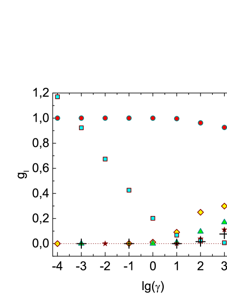
Fig. 1: [Color online] Coefficients $g_{1}$ (circles), $g_{2}$ (diamonds), $g_{3}$ (triangles), $g_{4}$ (stars), $g_{5}$ (crosses), and $g_{l_{m}}\equiv\tilde{\epsilon}=\epsilon/[2\bar{\rho}c(1-N^{-1})]$ (squares) obtained within the GP approach for the first stationary excited state of the condensate $\Phi_{j_{0}=2}(x)$ for $N=2$, $\bar{\rho}=1$, and various $\gamma$’s. Instead of $g_{l_{m}}$, the values of $\lg(g_{l_{m}})/4$ are given. The values of all $g_{l}$ obtained for $\gamma=10^{4}$ practically coincide with the seed ones $g_{l<l_{m}}=\frac{2\sqrt{2}}{\pi(2l-1)}$, $g_{l_{m}}=1$. The dotted line marks the zero level, $g_{l}=0$. In the GP approach, exactly the same solutions $g_{l}(\gamma)$ are obtained for $j_{0}=3,4,\ldots$ if $N=j_{0}$ (in this case, $g_{l}$ depend on $\gamma=c/\bar{\rho}$, but do not on $c$ and $\bar{\rho}$ separately; see equations (51) and (52) in [1]).

3 Main hypothesis

It is impossible to compare the solution $\Phi_{j_{0}}(x)$ (10) with all exact Bethe-ansatz solutions because their number is infinite. However, we may try to intuitively guess which exact solution corresponds to the function $\Phi_{j_{0}}(x)$.

We proceed from the fact that each solution of Eq. (7) or (8) describes a state where all $N$ atoms are in the condensate. We know that $\Phi_{1}(x)$ describes the ground state and corresponds to the exact Bethe-ansatz solution for [1] $n_{1}=n_{2}=\ldots=n_{N}=j_{0}=1$ (or $n_{p\leq N}=j_{0}=1$ for short). The states $\Phi_{j\geq 2}(x)$ describe the excited states of the condensate. Knowing the complete $N$-particle wave function, which is a solution of the exact $N$-particle Schrödinger equation, one can represent each excited state of the system as a set of interacting elementary excitations [35, 36]. Each $\Phi_{j_{0}\geq 2}(x)$ describes a state with the maximum possible number (i.e. $N$) of atoms in the condensate and therefore must correspond to a peculiar ensemble of elementary excitations that forms such a condensate of atoms. It is natural to assume that $\Phi_{j_{0}\geq 2}(x)$ corresponds to a state with the maximum possible number of identical elementary excitations. In this case, it is as if the excitations focus the atoms in a single-particle state that corresponds to the structure of these excitations. In sections 6 and 7 we will show that $\Phi_{j_{0}\geq 2}(x)$ corresponds to the exact Bethe-ansatz solution with $n_{p\leq N}=j_{0}$, which describes a condensate of $N$ identical elementary excitations, each of which has the quasimomentum $\pi(j_{0}-1)/L$.

Fig. 2: [Color online] System energy $E(\gamma)$ calculated for $N=2$ and $\bar{\rho}=1$ in different approaches: the energies $E_{\mathrm{GP}}$ (circles) and $E_{\mathrm{GP_{N}}}$ (diamonds) for the state $\Phi_{j_{0}=2}(x)$, and the exact Bethe-ansatz solution for $n_{p\leq N}=j_{0}=2$ (crosses). The solid line marks the energy $E=N(j_{0}\pi/L)^{2}$ of $N$ free particles for $j_{0}=2$.

Fig. 3: [Color online] Particle density profile $\rho(x)$ found for $N=2$ and $\bar{\rho}=1$ in various approaches: the GP solutions for the state $\Phi_{2}(x)$ at $\gamma=10^{-4}$ (triangles), $1$ (stars), $10$ (diamonds), $100$ (crosses); the exact Bethe-ansatz solution for $n_{1}=n_{2}=j_{0}=2$ and $\gamma=1$ (solid curve), $\gamma=10$ (dotted curve). The free-particle solution $\rho(x)=2\bar{\rho}\sin^{2}{(j_{0}\pi x/L)}$ for $j_{0}=2$ and the exact Bethe-ansatz solution for $\gamma=10^{-4}$ virtually coincide with the curve marked with triangles and therefore are not shown.

4 Two-domain state: $j_{0}=2$

In this section we study the solution $\Phi_{2}(x)$ which describes the first excited state of the condensate ($j_{0}=2$). The method of numerical solution of the GP (7) (or GP_N (8)) equation satisfying BCs (9) and the normalization condition $\int_{0}^{L}dx|\Phi(x)|^{2}=N$ is described in work [1]. We will see below that the solution $\Phi_{2}(x)$ at $N=2$ corresponds to a perfect crystal composed of two atoms, and at $N\gg 1$ it corresponds to a Lieb’s “hole-like” quasiparticle [37]. For what follows it is convenient to denote $b_{j_{0}(2l-1)}=\sqrt{N}f_{j_{0}(2l-1)}=\sqrt{N}g_{l}$ and write $\Phi_{j_{0}}(x)$ (10) in the form [1]

$$\Phi_{j_{0}}(x)=\sqrt{2\bar{\rho}}\sum\limits_{l=1,2,\ldots,\infty}g_{l}\sin[\pi j_{0}(2l-1)x/L].$$ (14)

The function $\Phi_{j_{0}}(x)$ is periodic with the period $\triangle x=2L/j_{0}$.

4.1 Solution for $N=2$

Consider the case $N=j_{0}=2$ and $\bar{\rho}=1$. The solutions for the coefficients $g_{l}$ from Eq. (14) for different $\gamma$’s are shown in Fig. 1. The dependence of $g_{l}$ on $\gamma$ is similar to that for the ground state (see [1]). The figure shows the solutions calculated only in the GP approach; the GP_N solutions are similar.

The dependences $E(\gamma)$ are shown in Figs. 3 and 10(a); they are similar to $E(\gamma)$ for the ground state [1]. Note that if $\gamma\ll 1$, the energies $E_{\mathrm{GP}}$ and $E_{\mathrm{GP}_{N}}$ [formula (11) with $q=1$ and $q=1-1/N$, respectively] are close to the exact energy $E_{\mathrm{Bethe}}$ (12) for $n_{p\leq N}=j_{0}$. In this case, $E_{\mathrm{GP}_{N}}$ coincides with $E_{\mathrm{Bethe}}$ with high accuracy.

Figure 3 demonstrates the particle density profile $\rho(x)=|\Phi_{j_{0}}(x)|^{2}$ [1] for the GP solution $\Phi_{2}(x)$ at $N=2$, $\bar{\rho}=1$, and different $\gamma$’s. The GP_N solution gives very close profiles; they are not shown because they would be visually indistinguishable from the GP profiles. One sees that $\rho(x)$ has a two-domain structure. For $\gamma\leq 1$, the profile $\rho(x)$ is close to the free-particle profile $\rho(x)=2\bar{\rho}\sin^{2}{(j_{0}\pi x/L)}$ and to the exact $\rho(x)$-solution [38] found by the Bethe ansatz. The GP solution $\rho(x)$ differs from the exact one in that the GP solution vanishes at $x=0;L/2;L$, whereas the exact solution only at $x=0;L$ (the both properties hold for all examined values of $\gamma$: $10^{-4}\leq\gamma\leq 100$).

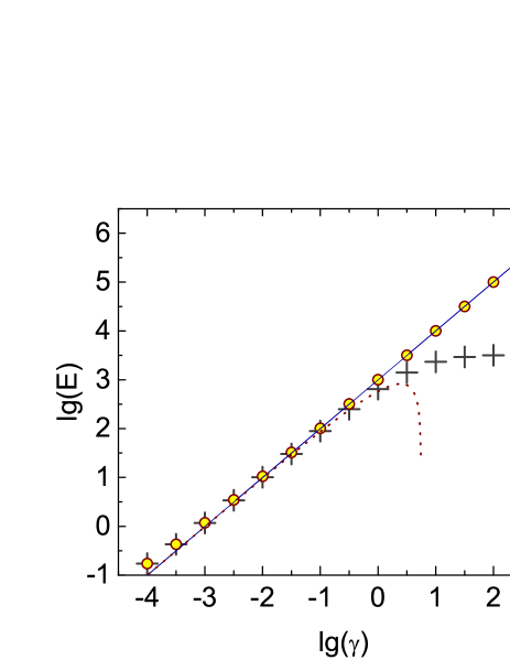
Fig. 4: [Color online] System energy $E(\gamma)$ calculated for $N=10^{3}$ and $\bar{\rho}=1$ by different methods: $E_{\mathrm{GP}_{N}}$ for the state $\Phi_{2}(x)$ (circles), the exact energy $E_{\mathrm{Bethe}}$ for $n_{j\leq N}=j_{0}=2$ (crosses), and the Bogoliubov ground-state energy $E_{0}=N\bar{\rho}^{2}\gamma\left(1-\frac{4\sqrt{\gamma}}{3\pi}\right)$ (dotted curve). The solid line shows the dependence $E=N\bar{\rho}^{2}\gamma$.

4.2 Solution for $N=1000$

The $E_{\mathrm{GP}_{N}}(\gamma)$ curves for the state $\Phi_{2}(x)$ for $N=1000$ are shown in Fig. 4. The GP approach gives close solutions that would be visually indistinguishable from the GP_N ones. One can see that at $\gamma\lesssim 0.1$, the energy $E_{\mathrm{GP}_{N}}$ is close to the exact energy $E_{\mathrm{Bethe}}$ for $n_{j\leq N}=j_{0}=2$. It is interesting that at $\gamma\lesssim 0.1$, the energy $E_{\mathrm{GP}_{N}}$ in Fig. 4 is close to the Bogoliubov energy of the ground state. This is probably due to the fact that at $\gamma\lesssim 0.1$ the function $\Phi_{2}(x)$ changes smoothly (see Fig. 6), so that the kinetic energy is low and the total energy of the system is mostly potential. At $\gamma\lesssim 0.1$ the latter is close to the Bogoliubov energy $E_{0}$, which is also mostly potential.

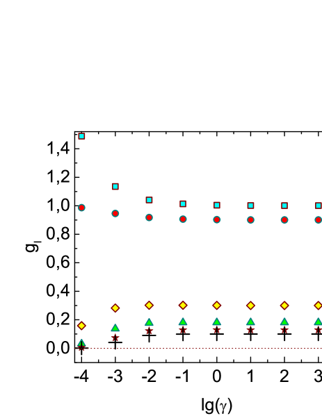
Fig. 5: [Color online] Coefficients $g_{1}$ (circles), $g_{2}$ (diamonds), $g_{3}$ (triangles), $g_{4}$ (stars), $g_{5}$ (crosses), and $g_{l_{m}}\equiv\tilde{\epsilon}$ (squares) obtained within the GP approach for the state $\Phi_{2}(x)$ at $N=1000$, $\bar{\rho}=1$, and different $\gamma$’s. In contrast to Fig. 1, the values of $g_{l_{m}}$ (instead of $\lg(g_{l_{m}})/4$) are shown. When $\lg(\gamma)\gtrsim 0$ the values of the coefficients $g_{l}$ practically coincide with $g_{l<l_{m}}=\frac{2\sqrt{2}}{\pi(2l-1)}$, $g_{l_{m}}=1$. The dotted line marks the zero level $g_{l}=0$.

The values of the coefficients $g_{l}$ for various $\gamma$’s are shown in Fig. 5. The $g_{l}(\gamma)$ curves for all $l$ are close to their ground-state counterparts for $N=1000$, see [1]. The figure shows only the solutions obtained in the GP approach, because the GP_N solutions are very close.

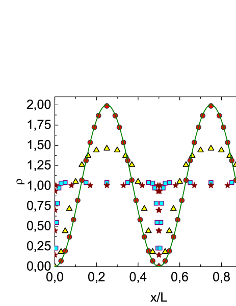
Fig. 6: [Color online] Particle density profiles $\rho(x)=|\Phi_{2}(x)|^{2}$ obtained in the GP approach for $N=1000$, $\bar{\rho}=1$, and $\gamma=10^{-6}$ (circles), $10^{-4}$ (triangles), $10^{-2}$ (squares), $1$ (stars). The solid line marks free particle curve $\rho(x)=2\bar{\rho}\sin^{2}{(j_{0}\pi x/L)}$ for $j_{0}=2$, $\bar{\rho}=1$.

Figure 6 shows the particle density profiles $\rho(x)=|\Phi_{j_{0}}(x)|^{2}$ for the GP solution $\Phi_{2}(x)$ at $N=1000$ and various $\gamma$’s. The GP_N solution gives a very close $\rho(x)$. As in Fig. 3, the $\rho(x)$ curve has a two-domain structure, and for $\gamma N^{2}\lesssim 1$ (the regime of near-free particles [1]) it is close to the free particle curve $\rho(x)=2\bar{\rho}\sin^{2}{(j_{0}\pi x/L)}$.

Figures 3, 10(a), 3, and 4 indicate that for $N=2(1000)$ and $\gamma\lesssim 0.1$, the solution $\Phi_{2}(x)$ corresponds to the exact Bethe-ansatz solution for $N=2(1000)$ and $n_{j\leq N}=2$. In section 7 we will see that the numbers $n_{j\leq N}=2$ correspond to the Lieb’s “hole”. As can be seen from Figs. 3 and 6, these are solutions with two-domain profiles $\rho(x)$. A Bethe-ansatz solution with a two-domain profile $\rho_{N}(x_{N})$ was previously obtained in work [39] for a periodic 1D system of spinless bosons.

Fig. 7: [Color online] The energy $E(\gamma)$ of the crystal-like excited state of the system obtained by different methods for $N=L=1000$ (the value of $E$ is divided by $10^{4}$): the energy $E_{\mathrm{GP}_{N}}(\gamma)$ of the state $\Phi_{j_{0}=N}(x)$ (circles); the exact energy $E_{\mathrm{Bethe}}(\gamma)$ for $n_{j\leq N}=j_{0}=N$ (crosses); the solid line marks the dependence $E(\gamma)=N(j_{0}\pi/L)^{2}$ for the system of $N$ free particles for $j_{0}=N$.

Fig. 8: [Color online] Particle density profiles $\rho(x)=|\Phi_{1000}(x)|^{2}$ for the crystal-like excited state of the condensate calculated in the GP_N approach for $j_{0}=N=L=1000$ and $\gamma=10^{-2}$ (squares), $1$ (stars), and $10^{2}$ (crosses). The solid line marks the free-particle curve $\rho(x)=2\bar{\rho}\sin^{2}{(j_{0}\pi x/L)}$ for $j_{0}=1000$, $\bar{\rho}=1$; with a high accuracy, it coincides with the curve marked by squares.

5 Solution for a perfect crystal: $j_{0}=N$

Figures 8 and 8 show solutions for the excited state $\Phi_{j_{0}}(x)$ of the condensate for $j_{0}=N=1000$. In the GP approach, the coefficients $g_{l}(\gamma)$ for $j_{0}=N=1000$ coincide with their counterparts for $j_{0}=N=2$ (see Fig. 1) because of the scaling properties of the system of equations for $g_{l}$ [1]. In the GP_N approach, those equations contain an additional factor $1-1/N$, which violates the scaling.

It is clear from Fig. 8 that if $\gamma\lesssim 0.1$, the energy $E_{\mathrm{GP}_{N}}$ is close to the exact energy $E_{\mathrm{Bethe}}$ obtained for the quantum numbers $n_{j\leq N}=j_{0}=N$. The energy $E_{\mathrm{GP}}$ is very close to $E_{\mathrm{GP}_{N}}$.

The particle density profiles $\rho(x)$ calculated for $N=L=1000$ and different $\gamma$’s (see Fig. 8) show that this solution corresponds to a perfect crystal with one atom per a lattice site. The system occupies the interval $x\in[0,L]=[0,1000]$, and Fig. 8 demonstrates the first five sites (domains). All $N$ domains are identical, i.e. they are a repetition in space of the first domain (with $\rho(x)=0$ at the points $x=0,1,2,\ldots,L-1,L$). Such properties result from the fact that when $x$ is replaced by $x+L/j_{0}$, the function $\Phi_{j_{0}}(x)$ (14) does not change its magnitude but changes its sign. Therefore, $\rho(x)=|\Phi_{j_{0}}(x)|^{2}$ is periodic with the period $\triangle x=L/j_{0}=1$.

Thus, the solution $\Phi_{2}(x)$ for $N=2$ corresponds to a perfect crystal consisting of two atoms, and $\Phi_{1000}(x)$ for $N=1000$ corresponds to a perfect crystal of 1000 atoms. The solution $\Phi_{2}(x)$ is close to the exact one for $\gamma\lesssim 1$ in the GP_N approach, and for $\gamma\lesssim 0.1$ in the GP one, whereas the solution $\Phi_{1000}(x)$ is close to the exact one for $\gamma\lesssim 0.1$ in both approaches.

Some approximate crystalline solutions with a condensate of atoms have already been found in the literature [40, 41, 42, 43, 44, 45, 46, 47, 48, 49]. The exact crystalline solution for a 1D few-boson system with point interaction was obtained in [38], and it corresponds to the solution $\Phi_{j_{0}=N}(x)$ above. Its energy is always higher than the energy of the ground state (the latter corresponds to a liquid); therefore, such a crystal is not a supersolid. If the interatomic potential is non-point, the crystalline solution may correspond to the ground state of the system.

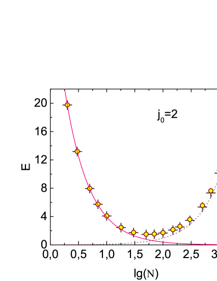
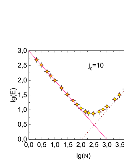
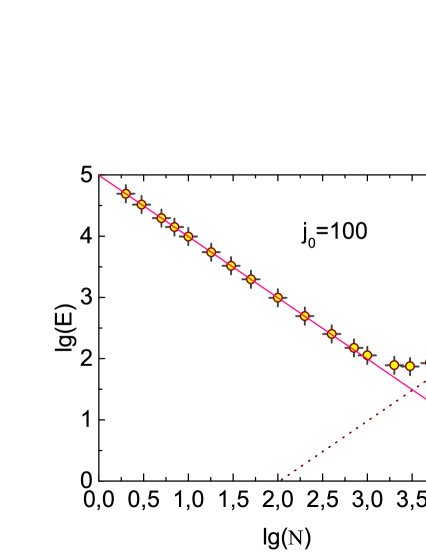
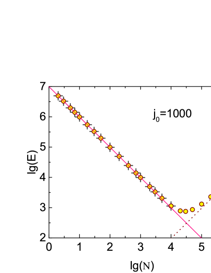
Fig. 9: [Color online] The dependence $E(N)$ for $c=0.01$, $\bar{\rho}=1$, and $j_{0}=2,10,100,1000$, calculated with different methods: the energy $E_{\mathrm{GP}}(N)$ of the condensate state $\Phi_{j_{0}}(x)$ (circles), the exact energy $E_{\mathrm{Bethe}}(N)$ for the state with $n_{j\leq N}=j_{0}$ (crosses), the Bogoliubov ground-state energy $E_{0}(N)=N\bar{\rho}^{2}\gamma\left(1-\frac{4\sqrt{\gamma}}{3\pi}\right)$ (dotted curves), and the energy of $N$ free particles $E(N)=N(j_{0}\pi/L)^{2}$ (solid curves). In the panel corresponding to $j_{0}=1000$, the solution $E_{\mathrm{Bethe}}$ is shown only for $N\leq 10^{4}$ (we were unable to solve the Gaudin’s equations (13) for $N>10^{4}$ due to the large computing time).

6 Correspondence between the solutions of the Gross-Pitaevskii equation and the exact Bethe-ansatz solutions

In work [1] it was shown that the solution $\Phi_{1}(x)$ of the GP (GP_N) equation, corresponding to the ground state of condensate, for $\gamma\lesssim 0.1$ coincides with the exact Bethe-ansatz solution with the quantum numbers $n_{j\leq N}=j_{0}=1$ (the latter solution corresponds to the ground state of the system for any $\gamma\geq 0$ [33, 50, 51]). Which quantum numbers $(n_{1},\ldots,n_{N})$ in the Bethe-ansatz approach correspond to the solutions $\Phi_{j_{0}>1}(x)$? The dependences $E(\gamma)$ and $E(N)$ (see Figs. 3, 4, 8, and 9) show that if $N<10$, the solution $\Phi_{j_{0}>1}(x)$ should correspond to the exact solution with $n_{j\leq N}=j_{0}$. For $N\gtrsim 10$, the energy $E$ of the system determined in the GP and GP_N approaches has a rather large error. As a result, the solution $\Phi_{j_{0}>1}(x)$ can be assigned both to the state with $n_{j\leq N}=j_{0}$ and to other $\{n_{j}\}$-states with similar energies.

Fig. 9 shows some interesting properties. First, when $N\lesssim 10j_{0}$, the energy $E_{\mathrm{GP}}$ is very close both to the exact energy $E_{\mathrm{Bethe}}$ and the energy of $N$ free particles $E=N(j_{0}\pi/L)^{2}$ [in this Section, $E_{\mathrm{Bethe}}$ does not denote the Bethe-ansatz energy of any ($n_{1},n_{2},\ldots,n_{N}$)-state, but only of the state with $n_{j\leq N}=j_{0}$, where $j_{0}$ is the same as in $\Phi_{j_{0}}(x)$]. Those two properties are apparently related to the fact that at $c=0.01$, $\bar{\rho}=1$, and $N\lesssim 10j_{0}$ the regime of near-free particles (see [1]) is realized. One can also see from Fig. 9 that when $N\gtrsim 100j_{0}$, the energy $E_{\mathrm{GP}}$ is close to the Bogoliubov ground-state energy, although $E_{\mathrm{GP}}$ corresponds to a highly excited state of the system. This strange property can be explained as follows. The solution $\Phi_{j_{0}}(x)$ corresponds to $j_{0}$ domains. The inequality $N\gtrsim 100j_{0}$ means that each domain contains more than 100 atoms. A numerical analysis shows that in this case the main contribution to $E_{\mathrm{GP}}$ is given by the potential energy of interatomic interaction (i.e. by uniform intradomain regions rather than interdomain ones with a high kinetic energy), which is similar to the Bogoliubov ground state. We found such properties to be valid for all examined values of $j_{0}$ and $N$.

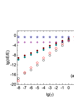
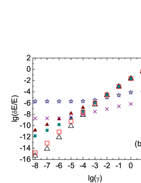
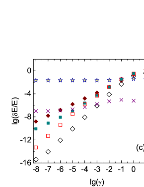
Fig. 10: [Color online] Errors of the GP and GP_N methods for the excited states $\Phi_{j_{0}>1}(x)$ at $\bar{\rho}=1$. (a) $\gamma$-Dependences of $\lg{\frac{E_{\mathrm{GP}}-E_{\mathrm{Bethe}}}{E_{\mathrm{Bethe}}}}$ for $N=10$ (solid diamonds) and $N=2$ (solid circles), $\lg{\frac{|E_{\mathrm{GP}_{N}}-E_{\mathrm{Bethe}}|}{E_{\mathrm{Bethe}}}}$ for $N=10$ (hollow diamonds ) and $N=2$ (hollow circles), and $\lg{\frac{E_{\mathrm{Bethe}}^{+}-E_{\mathrm{Bethe}}}{E_{\mathrm{Bethe}}}}$ for $N=2$ (stars) and $10$ (crosses). (b) $\gamma$-Dependences of $\lg{\frac{E_{\mathrm{GP}}-E_{\mathrm{Bethe}}}{E_{\mathrm{Bethe}}}}$ for $N=100$ (solid triangles) and $1000$ (solid squares), $\lg{\frac{|E_{\mathrm{GP}_{N}}-E_{\mathrm{Bethe}}|}{E_{\mathrm{Bethe}}}}$ for $N=100$ (hollow triangles ) and $1000$ (hollow squares), and $\lg{\frac{E_{\mathrm{Bethe}}^{+}-E_{\mathrm{Bethe}}}{E_{\mathrm{Bethe}}}}$ for $N=100$ (asterisks) and $1000$ (crosses). In panels (a) and (b), each of $E_{\mathrm{GP}}$, $E_{\mathrm{GP}_{N}}$, $E_{\mathrm{Bethe}}$, and $E_{\mathrm{Bethe}}^{+}$ corresponds to $j_{0}=N$. (c) $\gamma$-Dependences of $\lg{\frac{|E_{\mathrm{GP}_{N}}-E_{\mathrm{Bethe}}|}{E_{\mathrm{Bethe}}}}$, $\lg{\frac{E_{\mathrm{GP}}-E_{\mathrm{Bethe}}}{E_{\mathrm{Bethe}}}}$, and $\lg{\frac{E_{\mathrm{Bethe}}^{+}-E_{\mathrm{Bethe}}}{E_{\mathrm{Bethe}}}}$ for $N=10$ and $j_{0}=3$ (hollow diamonds, solid diamonds, and stars, respectively), and for $N=1000$ and $j_{0}=135$ (hollow squares, solid squares, and crosses, respectively). The quantum numbers $n_{p}$ for the exact solutions $E_{\mathrm{Bethe}}$ and $E_{\mathrm{Bethe}}^{+}$ are given in the text (see section 6).

Since $\Phi_{1}(x)$ is reliably identified as the ground state, the quantity $\frac{|E_{\mathrm{GP}_{N}}-E_{\mathrm{Bethe}}|}{E_{\mathrm{Bethe}}}$ for $\Phi_{1}(x)$ [1] virtually determines the accuracy of the GP_N approach. Figure 10 shows that the values of this quantity for all studied excited states are smaller than its value for the ground state (see Fig. 7 in [1]) provided the same $N=2$, $10$, $100$, $1000$ and the same $\gamma\lesssim 0.1$. This fact indicates that in the case $\gamma\lesssim 0.1$, the solution $\Phi_{j_{0}>1}(x)$ coincides with the Bethe-ansatz solution for $n_{j\leq N}=j_{0}$ within the error limits of the GP_N approach.

In addition, Fig. 10 shows the values of $E_{\mathrm{Bethe}}^{+}-E_{\mathrm{Bethe}}$ for different $\gamma$’s. Here $E_{\mathrm{Bethe}}^{+}$ is the energy of the state ($n_{1}=j_{0}-1,n_{2}=n_{3}=\ldots=n_{N-1}=j_{0},n_{N}=j_{0}+1$) [if $N=2$, then $n_{1}=j_{0}-1,n_{N}=j_{0}+1$]. A numerical analysis shows that for any $N\geq 2$ and $j_{0}>1$, the level $E_{\mathrm{Bethe}}^{+}$ is one of the closest (by energy) to the level $E_{\mathrm{Bethe}}$. For each $N\geq 2$, there are Bethe-ansatz states whose energy $E$ is closer to the level $E_{\mathrm{Bethe}}$ at a given $\gamma\lesssim 1$ (the number of such states is of the order of $Nj_{0}$; in this case, $\left|E-E_{\mathrm{Bethe}}\right|\sim|E_{\mathrm{Bethe}}^{+}-E_{\mathrm{Bethe}}|$ as a rule, although $\left|E-E_{\mathrm{Bethe}}\right|\ll|E_{\mathrm{Bethe}}^{+}-E_{\mathrm{Bethe}}|$ for some levels). It is clear that if $\left|E_{\mathrm{GP}_{N}}-E_{\mathrm{Bethe}}\right|\ll|E-E_{\mathrm{Bethe}}|$ for all Bethe-ansatz levels $E$ that are close to $E_{\mathrm{Bethe}}$, then the GP_N approach describes a state which exactly coincides with the state $n_{j\leq N}=j_{0}$ of the Bethe-ansatz approach. For $N\leq 5$ and $\gamma\lesssim 1$, we have numerically verified that $\left|E_{\mathrm{GP}_{N}}-E_{\mathrm{Bethe}}\right|\ll|E-E_{\mathrm{Bethe}}|$ indeed for all Bethe-ansatz levels $E$ and all $j_{0}=2,3,\ldots,1000$. When $N>5$, the computing time was too long, so we could not verify all required Bethe-ansatz levels.

Important additional information is provided by the profile $\rho(x)$. When $\gamma\rightarrow 0$, the Bethe-ansatz for any state $\{n_{j}\}$ can be written as $\Psi(x_{1},\ldots,x_{N})=(2i)^{N}\sum_{\sigma}\prod_{j=1}^{N}\sin(k_{\sigma(j)}x_{j})$ with $k_{\sigma(j)}=\pi n_{\sigma(j)}/L$ [52], and $\Phi_{j_{0}}(x)$ is reduced to $b_{j_{0}}\sqrt{2/L}\,\sin(k_{j_{0}}x)$ (see Figs. 1, 5 above). This implies that the domain structure of the profile $\rho(x)$ of the solution $\Phi_{j_{0}}(x)$ for $\gamma=0$ is reproduced only by the profile $\rho(x)$ of the exact Bethe-ansatz solution for $n_{j\leq N}=j_{0}$. If $\gamma>0$ the picture is less obvious. However, our analysis in this paper (see Fig. 11) and in [38] shows that when $\gamma>0$ the conclusion is the same (in this case the profile $\rho(x)$ of the solution $\Phi_{j_{0}}(x)$ consists of $j_{0}$ identical domains, whereas the profile of the Bethe-ansatz solution for $n_{j\leq N}=j_{0}$ consists of $j_{0}$ almost identical domains, with the difference between them being negligibly small if $\gamma\lesssim 1$). Even the nearest Bethe-ansatz sets $(n_{1}=j_{0}-1,n_{2}=\ldots=n_{N}=j_{0})$ and $(n_{1}=\ldots=n_{N-1}=j_{0},n_{N}=j_{0}+1)$ bring about the profiles $\rho(x)$ that differ considerably from the profile of the solution $\Phi_{j_{0}}(x)$, and the profiles $\rho(x)$ for other $\{n_{j}\}$-sets differ still more strongly from the latter; see Fig. 11 (for $N=2$ and $3$, this property was proven in this work and [38]; however, it is clear that it should hold for any $N\geq 2$).

For $N=10$ we found such Bethe-ansatz levels $E$ for which $\left|E-E_{\mathrm{Bethe}}\right|<|E_{\mathrm{Bethe}}^{+}-E_{\mathrm{Bethe}}|$. All these solutions had the quantum numbers $\{n_{j}\}$ that differed significantly from the set $n_{j\leq N}=j_{0}$ (this is also true for all similar $E$-levels at $N\leq 5$). As a result, the $\rho(x)$ profiles of such solutions should be very different from the GP_N profile consisting of $j_{0}$ identical domains. Hence, those solutions do not correspond to the GP_N solution. Therefore, for $N>5$, instead of finding all $E$-levels, we found only the level $E_{\mathrm{Bethe}}^{+}$, which is close to the level $E_{\mathrm{Bethe}}$ and has quantum numbers close to $n_{j\leq N}=j_{0}$.

The condition $\left|E_{\mathrm{GP}_{N}}-E_{\mathrm{Bethe}}\right|\ll E_{\mathrm{Bethe}}^{+}-E_{\mathrm{Bethe}}$ is satisfied if $\gamma N^{2}\lesssim 1$, i.e. in the near-free-particle regime (see Fig. 10). Taking into account the properties of the profile $\rho(x)$ that were described above, we arrive at the conclusion that for $\gamma N^{2}\lesssim 1$ the solution $\Phi_{j_{0}}(x)$ of the GP_N equation corresponds to the exact Bethe-ansatz solution with $n_{j\leq N}=j_{0}$, for any $N\geq 2$, $j_{0}=1,2,\ldots,\infty$, and $\gamma\lesssim 0.1$. For the values of $\gamma$ and $N$ that violate the relation $\gamma N^{2}\lesssim 1$, the inequality $\left|E_{\mathrm{GP}_{N}}-E_{\mathrm{Bethe}}\right|\ll E_{\mathrm{Bethe}}^{+}-E_{\mathrm{Bethe}}$ becomes invalid. However, this is apparently a result of the GP_N approach error: from the figures in this article and in [1], one sees that this error is very small if $\gamma N^{2}\lesssim 1$ but increases rapidly when moving away from this parameter region. The error of the GP approach exceeds the error of the GP_N approach, but the general conclusions for the GP approach are about the same.

It is also possible to find the nodal structure of the wave function $\Psi(x_{1},\ldots,x_{N})$, i.e. the set of cells into which the nodes of the wave function divide the space $(x_{1},\ldots,x_{N})$. In the GP (GP_N) approach we have $\Psi(x_{1},\ldots,x_{N})=\prod_{j=1}^{N}[\Phi_{j_{0}}(x_{j})/\sqrt{N}]$, and the expression for the Bethe ansatz $\Psi(x_{1},\ldots,x_{N})$ can be found in [1, 13, 33, 34]. In the cases $N=2$ and $N=3$, the nodal structure of the Bethe ansatz $\Psi(x_{1},\ldots,x_{N})$ was explored in [38]. It turned out that the nodal structure of the GP (GP_N) solution $\Psi(x_{1},\ldots,x_{N})$ for $j_{0}=N$ coincides with the nodal structure of only one Bethe ansatz $\Psi(x_{1},\ldots,x_{N})$, namely, the ansatz with $n_{j\leq N}=j_{0}$. If $N=2$ or $3$, it is easy to verify that this behavior holds for $j_{0}\neq N$ as well. It is clear that it should hold for all $N\geq 2$ and $j_{0}\geq 1$.

Thus, the analysis of the energy levels shows that every solution $\Phi_{j_{0}}(x)$ corresponds exactly to the Bethe-ansatz solution for $n_{j\leq N}=j_{0}$ and the same $N$ when $N\leq 5$. If $N>5$, our analysis of the energy levels only allows us to state that each solution $\Phi_{j_{0}}(x)$ corresponds to a set of Bethe-ansatz solutions: the solution for $n_{j\leq N}=j_{0}$ and other $(n_{1},\ldots,n_{N})$-solutions with very close energies. The nodal structure of the functions $\Psi(x_{1},\ldots,x_{N})$ and the properties of the profiles $\rho(x)$, which were explored for $N=2$ and $3$, show that each solution $\Phi_{j_{0}}(x)$ corresponds exactly to the Bethe-ansatz solution for $n_{j\leq N}=j_{0}$ and the same $N$. There is no doubt that in the case $N>3$ the properties of $\rho(x)$ and the nodal structures are also similar (although we have not proven this statement). Consequently, every solution $\Phi_{j_{0}}(x)$ corresponds exactly to the Bethe-ansatz solution for $n_{j\leq N}=j_{0}$ and the same $N$, for arbitrary $N\geq 2$ and $j_{0}\geq 1$.

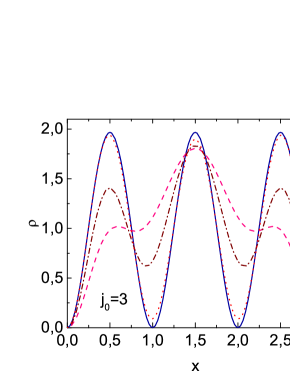
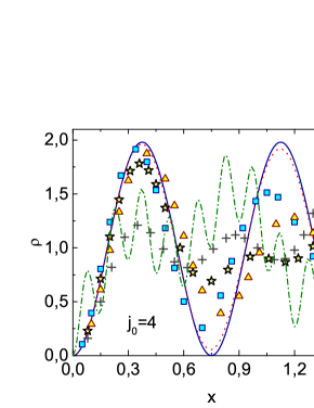
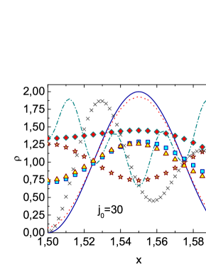
Fig. 11: [Color online] Particle density profiles $\rho(x)$ calculated for $N=L=3$, $\gamma=1$, and $j_{0}=3$, $4$, $30$ in different approaches: the GP_N solution for the state $\Phi_{j_{0}}(x)$ (solid curves), the exact Bethe-ansatz solutions for the states $n_{1}=n_{2}=n_{3}=j_{0}$ (dotted curves); $(n_{1}=j_{0}-1,n_{2}=j_{0},n_{3}=j_{0})$ [triangles]; $(n_{1}=j_{0},n_{2}=j_{0},n_{3}=j_{0}+1)$ [squares]; and $(n_{1}=j_{0}-1,n_{2}=j_{0},n_{3}=j_{0}+1)$ [stars]. The $\left(j_{0}=3\right)$-panel also shows the $\rho(x)$-profiles for the Bethe-ansatz states $(n_{1}=1,n_{2}=1,n_{3}=3)$ [dashed curve] and $(n_{1}=1,n_{2}=3,n_{3}=3)$ [dash-dotted curve]. The $\left(j_{0}=4\right)$-panel additionally shows the $\rho(x)$-profiles for the states $(n_{1}=1,n_{2}=3,n_{3}=5)$ [crosses] and $(n_{1}=2,n_{2}=5,n_{3}=20)$ [dash-dotted curve]; here $\rho(x)$ is shown in the interval $x\in[0,L/2]$; the profile in the interval $x\in[L/2,L]$ can be obtained using the formula $\rho(x)=\rho(L-x)$. The $\left(j_{0}=30\right)$-panel also demonstrates the $\rho(x)$-profile for the states $(n_{1}=40,n_{2}=50,n_{3}=60)$ [crosses], $(n_{1}=5,n_{2}=15,n_{3}=20)$ [diamonds], and $(n_{1}=3,n_{2}=31,n_{3}=120)$ [dash-dotted curve]; $\rho(x)$ is shown in the interval $x\in[1.5,1.6]$ corresponding to the 16th domain of the GP_N solution (the whole system is located within the interval $x\in[0,3]$). In all panels, the dotted curves almost coincide with the solid ones.

7 Elementary excitations

Let us find out which set of elementary collective excitations (elementary quasiparticles) corresponds to the state $n_{j\leq N}=j_{0}>1$. According to L. Landau’s idea, a system of many interacting particles at $T\rightarrow 0$ can be considered as a small number of free quasiparticles [53]. In a Bose system, several quasiparticles can be considered as a single one, so quasiparticles are introduced ambiguously: an infinite number of different quasiparticle ensembles can be associated with the same system. As an elementary excitation, one usually calls an indivisible quasiparticle, i.e. a quasiparticle that cannot be represented as several interacting quasiparticles. Intuitively, one may expect that the simplest formulae are obtained by describing a system in the language of elementary excitations.

Let us consider this issue in detail using the example of our 1D system of interacting spinless point bosons under zero BCs. Its ground state corresponds to the quantum numbers $n_{j\leq N}=1$ [33, 50, 51]. For excited states, any $n_{j}$ can take the values $n_{j}=1,2,3,\ldots,\infty$ [33, 51]. Consider the state ($n_{j\leq N-1}=1,n_{N}=r>1$). Its energy is higher than the energy $E_{0}$ of the ground state by a value of

$$E(p)=\sum\limits_{j=1}^{N}(|\acute{k}_{j}|^{2}-|k_{j}|^{2}),$$ (15)

where $\{|\acute{k}_{j}|\}$ and $\{|k_{j}|\}$ are the solutions of Gaudin’s equations (13) for the states $(n_{j\leq N-1}=1,n_{N}=r>1)$ and ($n_{j\leq N}=1$), respectively, and $p$ is the quasimomentum of a quasiparticle [54]

$$p=\sum\limits_{j=1}^{N}(|\acute{k}_{j}|-|k_{j}|)-\frac{1}{L}\sum\limits_{l,j=1}^{N}\left(\arctan{\frac{c}{|\acute{k}_{l}|+|\acute{k}_{j}|}}-\arctan{\frac{c}{|k_{l}|+|k_{j}|}}\right)|_{j\neq l}=\frac{\pi(r-1)}{L}.$$ (16)

Numerical calculations show that at $\gamma=1$ the curve $E(p)$ is close to the Bogoliubov curve (see Fig. 12), and at $\gamma\ll 1$ it is extremely close to the Bogoliubov curve (not shown in Fig. 12). Therefore, it is clear that at $\gamma\lesssim 1$ all states of the type $(n_{j\leq N-1}=1,n_{N}=r>1)$ correspond to the Bogoliubov quasiparticles.

Now consider the states of the type $(n_{j\leq N-2}=1,n_{N-1}=r_{2},n_{N}=r_{1})$ where $\left(r_{1},r_{2}\right)>1$. Similarly to the analysis above, it can be shown that the energy of such states is equal to $E_{0}+E(p_{1})+E(p_{2})+\delta E_{2}$, where $p_{1}=\pi(r_{1}-1)/L$, $p_{2}=\pi(r_{2}-1)/L$, and $\delta E_{2}$ is a small correction (always $\delta E_{2}<0$ and $|\delta E_{2}|\lesssim[E(p_{1})+E(p_{2})]/N$). It is natural to interpret $\delta E_{2}$ as the interaction energy of two quasiparticles corresponding to the states ($n_{j\leq N-1}=1,n_{N}=r_{1})$ and $(n_{j\leq N-1}=1,n_{N}=r_{2})$ of the system. Further, we can show that the state $(n_{j\leq N-3}=1,n_{N-2}=r_{3},n_{N-1}=r_{2},n_{N}=r_{1})$ with $\left(r_{1},r_{2},r_{3}\right)>1$ can be considered as three interacting quasiparticles corresponding to the states $(n_{j\leq N-1}=1,n_{N}=r_{1})$, $(n_{j\leq N-1}=1,n_{N}=r_{2})$, and $(n_{j\leq N-1}=1,n_{N}=r_{3})$. Whence it is not difficult to guess that any state of the type $(n_{j\leq N-i}=1,n_{N-i+1}=r_{i},\ldots,n_{N}=r_{1})$ is a set of $i$ interacting quasiparticles, where the first quasiparticle corresponds to the state $(n_{j\leq N-1}=1,n_{N}=r_{1})$, the second to the state $(n_{j\leq N-1}=1,n_{N}=r_{2})$, and so on, and the $i$-th particle to the state $(n_{j\leq N-1}=1,n_{N}=r_{i})$. If $i\sim N$, then the interaction energy $\delta E_{i}$ of quasiparticles is high and comparable to the energy $E(p_{1})+\ldots+E(p_{i})$. The properties described above are valid for any $\gamma>0$. Therefore, the state $n_{j\leq N}=j_{0}>1$ corresponds to a condensate of $N$ identical interacting quasiparticles, each of which corresponds to the state $(n_{j\leq N-1}=1,n_{N}=j_{0})$.

Is the quasiparticle $(n_{j\leq N-1}=1,n_{N}=j_{0}>1)$ an elementary excitation? This question is not quite trivial. There are two ways to answer it: (1) to explore the structure of the wave functions (WFs) or (2) to diagonalize the Hamiltonian. Let us consider these possibilities.

(1) For periodic BCs, any excited state of a system of spinless bosons with the momentum $\hbar\mathbf{p}$ can be described by the exact wave function [36, 55]

$$\Psi_{\mathbf{p}}(\mathbf{r}_{1},\ldots,\mathbf{r}_{N})=A_{\mathbf{p}}\psi_{\mathbf{p}}\Psi_{0},$$ (17)

where

$$\psi_{\mathbf{p}} = b_{1}(\mathbf{p})\rho_{-\mathbf{p}}+\sum\limits_{\mathbf{q}_{1}\neq 0}^{\mathbf{q}_{1}+\mathbf{p}\neq 0}\frac{b_{2}(\mathbf{q}_{1};\mathbf{p})}{2!N^{1/2}}\rho_{\mathbf{q}_{1}}\rho_{-\mathbf{q}_{1}-\mathbf{p}}+\sum\limits_{\mathbf{q}_{1},\ textbf{q}_{2}\neq 0}^{\mathbf{q}_{1}+\mathbf{q}_{2}+\mathbf{p}\not=0}\frac{b_{3}(\mathbf{q}_{1},\mathbf{q}_{2};\mathbf{p})}{3!N}\rho_{\mathbf{q}_{1}}\rho_{\mathbf{q}_{2}}\rho_{-\mathbf{q}_{1}-\mathbf{q}_{2}-\mathbf{p}}+$$ (18)

$$+ \ldots+\sum\limits_{\mathbf{q}_{1},\ldots,\mathbf{q}_{N-1}\neq 0}^{\mathbf{q}_{1}+\ldots+\mathbf{q}_{N-1}+\mathbf{p}\not=0}\frac{b_{N}(\mathbf{q}_{1},\ldots,\mathbf{q}_{N-1};\mathbf{p})}{N!N^{(N-1)/2}}\rho_{\mathbf{q}_{1}}\ldots\rho_{\mathbf{q}_{N-1}}\rho_{-\mathbf{q}_{1}-\ldots-\mathbf{q}_{N-1}-\mathbf{p}},$$

$\Psi_{0}$ is the ground-state wave function, $\mathbf{r}_{j}$ denote the atomic coordinates, $A_{\mathbf{p}}$ is a normalization constant, and $\rho_{\mathbf{q}}=\frac{1}{\sqrt{N}}\sum_{j=1}^{N}e^{-i\mathbf{q}\mathbf{r}_{j}}$ are collective variables. The values of the coefficients $b_{j}(\mathbf{p})$ show which state is described by function (17): with one, two, or $j$ interacting elementary excitations [36]. If this is one elementary excitation, then $b_{j}(\mathbf{p})\sim 1$ for all $j=1,\ldots,N$. In the case of $l$ excitations with the total momentum $\hbar\mathbf{p}=\hbar\mathbf{p}_{1}+\ldots+\hbar\mathbf{p}_{l}$, one needs to make the following changes in Eqs. (17) and (18): $\Psi_{\mathbf{p}}\rightarrow\Psi_{\mathbf{p}_{1}\ldots\mathbf{p}_{l}}$, $\psi_{\mathbf{p}}\rightarrow\psi_{\mathbf{p}_{1}\ldots\mathbf{p}_{l}}$, $A_{\mathbf{p}}\rightarrow A_{\mathbf{p}_{1}\ldots\mathbf{p}_{l}}$, and $b_{j}(\mathbf{q}_{1},\ldots,\mathbf{q}_{j-1};\mathbf{p})\rightarrow b_{j}(\mathbf{q}_{1},\ldots,\mathbf{q}_{j-1};\mathbf{p}_{1},\ldots,\mathbf{p}_{l},N)$ for all $j$. A solution in the case of two excitations ($l=2$) with the momenta $\hbar\mathbf{p}_{1}$ and $\hbar\mathbf{p}_{2}$ was found in paper [36]; in this case the following relationships have to be obeyed: $b_{j\geq 3}\sim 1$, $b_{1}(\mathbf{p}_{1},\mathbf{p}_{2},N)\sim N^{-1/2}$, $b_{2}(\mathbf{q}_{1};\mathbf{p}_{1},\mathbf{p}_{2},N)\sim N^{-1/2}$ for $\mathbf{q}_{1}\neq-\mathbf{p}_{1},-\mathbf{p}_{2}$, and $b_{2}(\mathbf{q}_{1};\mathbf{p}_{1},\mathbf{p}_{2},N)\sim N^{1/2}$ for $\mathbf{q}_{1}=-\mathbf{p}_{1},-\mathbf{p}_{2}$. The case $l>2$ can be considered analogously [36]. Thus, the structure of WFs (17) uniquely shows how many elementary excitations a given state contains. According to the analysis in works [36, 55], for a periodic system of spinless bosons, the elementary excitations are the Bogoliubov quasiparticles.

For zero BCs no solution of kind (17), (18) has been found.

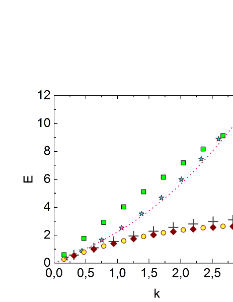
Fig. 12: [Color online] Dispersion laws $E(k)$ for quasiparticles of several types for a 1D system of spinless point bosons with zero boundary conditions and $N=1000$, $\bar{\rho}=1$, $\gamma=1$: 1) Dispersion law for the states ($n_{j\leq N-1}=1$, $n_{N}=r>1$) calculated using formulae (15), (16), and (13) (stars); 2) Bogoliubov law $E=\sqrt{k^{4}+4\gamma\bar{\rho}^{2}k^{2}}$ (dotted curve); 3) “dispersion curve” $\frac{E(k=p/(j_{0}-1))}{j_{0}-1}$ for a condensate of quasiparticles for $j_{0}=2$ (Lieb’s hole excitations, diamonds), $10$ (circles), $100$ (crosses), and $1000$ (squares); the condensate of quasiparticles is characterized by the quantum numbers $n_{j\leq i}=1$, $n_{j>i}=j_{0}$ (in this case, $N-i\gg 1$); see more details in the text.

(2) If the Hamiltonian of a system of spinless bosons is diagonalized and the creation and annihilation operators of quasiparticles satisfy the boson commutation relations, then such quasiparticles are elementary excitations. Indeed, any composite excitation must correspond to a creation operator of the form $\hat{B}_{\mathbf{k}}^{+}=\hat{b}_{\mathbf{k}_{1}}^{+}\cdots\hat{b}_{\mathbf{k}_{j}}^{+}$, where $\hat{b}_{\mathbf{k}_{1}}^{+},\ldots,\hat{b}_{\mathbf{k}_{j}}^{+}$ are the creation operators of elementary excitations $1,2,\ldots j$ that the composite excitation consists of. If the relation $\hat{b}_{\mathbf{k}_{i}}\hat{b}_{\mathbf{k}_{i}}^{+}-\hat{b}_{\mathbf{k}_{i}}^{+}\hat{b}_{\mathbf{k}_{i}}=1$ $(i=1,2,\ldots j)$ is satisfied, then it is easy to verify that the boson commutation relation $\hat{B}_{\mathbf{k}}\hat{B}_{\mathbf{k}}^{+}-\hat{B}_{\mathbf{\ k}}^{+}\hat{B}_{\mathbf{k}}=1$ is violated. Therefore, in particular, the Bogoliubov quasiparticles are elementary excitations.

The Hamiltonian of a 1D system of spinless bosons with zero BCs was diagonalized in work [56]; in this case all quasiparticles are the Bogoliubov ones. Since for a weak coupling the dispersion law and the quasimomentum $p=\pi(r_{1}-1)/L$ of the quasiparticles $(n_{j\leq N-1}=1,n_{N}=r_{1})$ considered above coincide with the dispersion law and the quasimomentum of the Bogoliubov quasiparticles, quasiparticles $(n_{j\leq N-1}=1,n_{N}=r_{1})$ are elementary excitations. In this case, there are no other elementary excitations in the system because any excited state $(n_{1},n_{2},\ldots,n_{N})$ can be considered as a set of interacting Bogoliubov quasiparticles. The state $n_{j\leq N}=j_{0}>1$ is a set of $N$ identical interacting elementary excitations $(n_{j\leq N-1}=1,n_{N}=j_{0})$.

It is generally accepted that elementary excitations of a 1D system of spinless point bosons are “particles” (Bogoliubov quasiparticles) and “holes”[37]. However, this is not quite so: the analysis above shows that, for a weak coupling, only Bogoliubov quasiparticles are elementary excitations of such a system. In work [36] it was shown in a different way, that for a weak coupling and periodic BCs, a hole is a composite quasiparticle: it is a set of identical interacting Bogoliubov phonons, each of which has the momentum $2\hbar\pi/L$.

In the Bethe-ansatz approach [50] and the Bogoliubov approach [57], the energy of any weakly excited state of a system with $N\gg 1$ is expressed by the formula

$$E=E_{0}+\sum\limits_{\mathbf{p}}N_{\mathbf{p}}E(\mathbf{p}),$$ (19)

where $E(\mathbf{p})$ is the energy of a Bogoliubov quasiparticle, and $N_{\mathbf{p}}$ is the number of quasiparticles. In this case, there is a one-to-one correspondence between weakly excited states in the Bethe-ansatz and Bogoliubov approaches. On the other hand, in the Bethe-ansatz approach, each state of the system can be formally considered as a set of interacting holes [36, 37], and a formula like (19) can be written for the holes. Hence, there exists a dualism between holes and Bogoliubov quasiparticles [36, 37]. Therefore, in order to find out which quasiparticles are elementary (indivisible) excitations, a more subtle analysis is required.

Such an analysis for a periodic system was carried out in Ref. [36], where the hole was as if zoomed in. In particular, a comparison was made between the solutions for holes with the momenta $2\hbar\pi/L$ and $4\hbar\pi/L$, on the one hand, and one- and two-phonon solutions obtained using WF (17), on the other hand. The structure of the corresponding wave functions, the correction to the one-phonon energy, and the magnitude of the two-phonon interaction energy clearly indicate [36] that for a weak coupling, a hole with the lowest momentum ($2\hbar\pi/L$) is a phonon, whereas a hole with the momentum $4\hbar\pi/L$ consists of two identical interacting phonons. It is therefore obvious that a hole with the momentum $j\cdot 2\hbar\pi/L$ is $j$ interacting identical phonons, each with the momentum $2\hbar\pi/L$. In other words, phonons (Bogoliubov quasiparticles) are elementary excitations. For a strong coupling, the system becomes fermion-like, a hole-like quasiparticle becomes similar to the fermion hole, and the separation into “particles” and holes is justified. At the same time, the properties of the system are strange: the structure of the WFs shows that apparently only two quasiparticles, $(0,0,\ldots,0,1)$ and $(-1,0,\ldots,0.0)$, are elementary excitations [36].

Under zero BCs, the hole-like quasiparticle corresponds to the quantum numbers $n_{1\leq j\leq i}=1$, $n_{i<j\leq N}=2$ (where $i=0,1,\ldots,N-2$ ) and the quasimomentum $p=\pi(N-i)/L$ [54]. Fig. 12 shows the dispersion law for hole-like quasiparticles, which was obtained using formula (15). The numbers $\{|\acute{k}_{j}|\}$ and $\{|k_{j}|\}$ were found by numerical solution of Gaudin’s equations (13). Similarly to the case of a system with periodic BCs, under zero BCs a hole with the quantum numbers $n_{1\leq j\leq i}=1$, $n_{i<j\leq N}=2$ is a set of $N-i$ interacting phonons, each with the quasimomentum $\pi/L$.

It is of interest to consider the states ($n_{j\leq i}=1,n_{j>i}=j_{0})$, where $i=0,1,\ldots,N-2$, which correspond to the sets of $N-i$ interacting phonons, each of which has the quasimomentum $(j_{0}-1)\pi/L$. Since the total quasimomentum of the system is defined by the formula [54]

$$P(\{|k_{i}|\})=\sum\limits_{j=1}^{N}|k_{j}|-\frac{1}{L}\sum\limits_{l,j=1}^{N}\arctan{\frac{c}{|k_{l}|+|k_{j}|}}|_{j\neq l}=\frac{\pi}{L}\sum\limits_{j=1}^{N}n_{j},$$

the ground state corresponds to the quasimomentum $\pi N/L$, and the state $(n_{j\leq i}=1$, $n_{j>i}=j_{0})$ can effectively be considered as a single “excitation” with the quasimomentum $p=(N-i)(j_{0}-1)\pi/L$. Using formula (15) it is easy to numerically find the energy $E$ of such a “quasiparticle”. The dependence of the quantity $E^{\prime}=\frac{E}{j_{0}-1}$ on $k=\frac{p}{j_{0}-1}$ for various $j_{0}$’s is shown in Fig. 12. One can see that if $j_{0}\lesssim 100$, the explored dependence is close to the hole dispersion law (at $j_{0}=2$ this dependence is the hole dispersion law). This curious property shows that a “dispersion law” similar to the hole one can also be obtained for a set of identical quasiparticles, each of which has the quasimomentum $(j_{0}-1)\pi/L$. The state $n_{j\leq N}=j_{0}>1$ considered in the previous sections corresponds to a set of $N$ such quasiparticles (the last point in the curves $E^{\prime}(k)$ in Fig. 12). Note that the deviation of the “dispersion curves” $E^{\prime}(k)$ as $k$ increases from the asymptotes $E(k\rightarrow 0)=const\cdot k$ is associated with the strengthening of the interaction between the quasiparticles forming this state. Similarly, as $N$ increases, the total interaction of atoms increases, which leads to the depletion of the condensate and a decrease in the accuracy of the GP method. In this sense the bending of the curve $E^{\prime}(k)$ with increasing $k$ and the increase in the value of $\frac{E_{\mathrm{GP}_{N}}-E_{\mathrm{Bethe}}}{E_{\mathrm{Bethe}}}$ with increasing $N$ (Fig. 10) are kindred.

In the previous sections we saw that the state $n_{j\leq N}=j_{0}>1$ corresponds to the profile $\rho(x)$ with $j_{0}$ domains. A region between adjacent domains is similar to a soliton [7, 11]: it is a black soliton in the GP (GP_N) approach and a dark soliton in the Bethe-ansatz approach. In particular, the hole quasiparticle with quantum numbers $n_{j\leq N}=2$ corresponds to two domains and one soliton. Soliton-like properties of hole quasiparticles were studied in works [3, 39, 58, 59, 60, 61, 62], see also review [13]. In the work [52] by A. Syrwid and K. Sacha (see also [13]), it was already found that the particle density profile for the state $n_{j\leq N}=j_{0}>1$ has a $j_{0}$-domain structure, but a relationship with the solutions of the GP equation has not been explored. Note that a hole is a soliton-like structure only if its momentum (quasimomentum) is large enough, i.e. if it is comparable to the maximum possible value. If the hole momentum is small, then a hole is a set of a small number of interacting phonons and is not a soliton: It is obvious without calculations that several identical phonons with the smallest momentum (quasimomentum) in a system with a very large $N$ should produce a non-soliton density profile very close to $\rho(x)=\mathrm{const}$. In this case, such a state is a Lieb’s hole.

Finally, note that the choice of quasiparticles determines the statistics. The WFs of a Bose system are always Bose-symmetric with respect to atomic permutations. But the energy distribution of quasiparticles and the commutation relations for the operators of creation and annihilation of quasiparticles depend on the method of introducing quasiparticles. Since quasiparticles can be introduced in an infinite number of ways, the number of statistics is also infinite. As was remarked above, elementary quasiparticles for a system of spinless bosons with weak coupling are Bogoliubov quasiparticles. If the system is one-dimensional and the interaction is point-like, the partition function can be summed exactly for $N=\infty,L=\infty$ and $T\rightarrow 0$, which leads to a formula for the free energy of a system of free Bose quasiparticles, for any coupling constant $\gamma>0$ [50]. In general, the simplest statistical description of a system of interacting bosons at $T\rightarrow 0$ is obtained if the system is considered as an ideal gas of elementary excitations. A more complicated thermodynamic approach was proposed by C.N. Yang and C.P. Yang [63]. This is a universal single-particle approach. At $T\rightarrow 0$ this approach is equivalent to the Bose-quasiparticle approach, as shown in Ref. [64]. Based on the Yang–Yang approach, it was found that at any $T$, a system of interacting point bosons can be statistically considered as a system of free particles with a generalized fractional statistics [65, 66] (see also [67]). It is essential that the approach in Refs. [65, 66] is single-particle and has no relevance to collective excitations.

8 Discussion

Above we considered the states $n_{j\leq N}=j_{0}>1$, which correspond simultaneously to a condensate of atoms and a condensate of elementary quasiparticles. Using the Bethe ansatz, it is easy to write down states with several condensates of quasiparticles. For example, the state $(n_{1}=n_{2}=\ldots=n_{j=10^{6}}=r_{1},n_{j=10^{6}+1}=\ldots=n_{j=2\times 10^{6}}=r_{2},n_{j=2\times 10^{6}+1}=\ldots=n_{j=3\times 10^{6}=N}=r_{3})$, where $r_{1},r_{2},r_{3}>1$, $r_{1}\neq r_{2},r_{3}$, and $r_{2}\neq r_{3}$, corresponds to three condensates of quasiparticles (and three condensates of atoms, if $\gamma$ is small). But such states can scarcely be obtained experimentally and cannot be described by the Gross-Pitaevskii equation.

Condensates of photons [68], excitons [69, 70, 71], exciton polaritons [72, 73, 74, 75], and magnons [76, 77, 78, 79, 80] have already been obtained experimentally (see also review [81]). The possibility of condensation of rotons [82] and phonon pairs [83] was argued.

In work [83] an effectively one-dimensional Bose gas was considered, and it was shown that a periodic variation of the transverse trap frequency can create a condensate of pairs of phonons with opposite momenta $\mathbf{k}_{z},-\mathbf{k}_{z}$. This is a “doubly coherent” state: a condensate of atoms and a condensate of phonon pairs. In this approach, in contrast to our solution, an external field is required for the condensate of quasiparticles to exist, pairs of quasiparticles are condensed instead of single quasiparticles, and the number of phonons in the condensate is much smaller than $N$ (this is evident from the fact that the condensate of quasiparticles changes the particle density $\rho(z)$ very little).

9 Concluding remarks

We have shown that for a 1D system of spinless point bosons under zero boundary conditions, each stationary excited state $\Phi_{j_{0}}(x)$ of a condensate of $N$ atoms contains a condensate of $N$ elementary excitations (Bogoliubov quasiparticles); we have proved this for the case $N\leq 5$ and argued for $N>5$. It is interesting that the solution $\Phi_{j_{0}}(x)$ has a $j_{0}$-domain density profile $\rho(x)$, and the region between neighbouring domains is a stationary black soliton (i.e. the solution contains $j_{0}-1$ identical black solitons).

Thus, any stationary excited state of a condensate of atoms is doubly coherent: it is simultaneously a condensate of atoms and a condensate of elementary excitations. From the other side, this means that for a weak coupling every state with a condensate of $N$ elementary excitations corresponds to a condensate of atoms. We have shown this for a 1D system with a point-like interatomic potential. However, it is natural to expect that this property is universal and holds true for a Bose system of any dimensionality, with any interatomic potential and any trap field (or any BCs in the absence of a trap).

Note that the solutions $\Phi_{j_{0}>1}(x)$ have already been obtained in the form of elliptic functions [26], and the soliton-like profile $\rho(x)$ for the Bethe-ansatz states $n_{j\leq N}=j_{0}>1$ has previously been found in [52]. However, a relation of these solutions to each other and to elementary quasiparticles has not been ascertained. This was done in the present work. It is also worth noting that the soliton-like behavior of the solutions $\Phi_{j_{0}>1}(x)$ is due to the condensate of elementary excitations. This can be verified by finding the particle density profile $\rho(x)$ within the Bethe-ansatz approach for a system with one, two, ten (say) and $N$ identical elementary excitations. The change in the profile with increasing number of identical excitations should show that the solitonic structure appears when the number of identical excitations becomes large [$\sim N$] (it is clear that for $N\gg 1$ several excitations give a non-soliton profile $\rho(x)$ which, far from the boundaries, is close to $\rho(x)=const$). This tendency can be seen even for $N=3$ (see Fig. 11, panel for $j_{0}=3$). It is clear that this statement should be true for large $N$, since many identical elementary excitations resonantly amplify the deviation of $\rho(x)$ from the constant. In this case the largest deviation should occur at the points corresponding to the oscillation maximum for each half-wave $\lambda/2=\pi/p=L/(j_{0}-1)$, which exactly corresponds to the structure of $\Phi_{j_{0}>1}(x)$. Thus, a $(j_{0}-1)$-fold dark soliton is a $N$-fold amplified phonon with the quasimomentum $\hbar\pi(j_{0}-1)/L$. It agrees with the result of work [83], according to which the condensate of phonon pairs produces a periodic particle density profile.

The doubly coherent states are soliton-like and can have a long lifetime. One can try to obtain them using an external alternating electromagnetic field in two ways: abruptly or gradually. In the first case, the field transforms the condensate, as a set of atoms, into the excited state $\Phi_{j_{0}}(x)$, and the field frequency must be equal to $(E_{j_{0}}-E_{1})/\hbar$, where $E_{j_{0}}$ and $E_{1}$ are the condensate energies for the states $\Phi_{j_{0}}(x)$ and $\Phi_{1}(x)$, respectively. In the second case, the external field acts on the system, as a set of quasiparticles, and gradually creates identical quasiparticles; the energy of the field quantum should be equal to the quasiparticle energy. In this case, because the number of identical quasiparticles increases and the energy of each quasiparticle decreases due to its interaction with other quasiparticles, the field frequency must be correspondingly lowered in time. The derivation [84] of the probability of the creation of a circular roton in He II by the field of a microwave resonator [85, 86] is related to the second mechanism.

It is clear that an experimentally obtained condensate of elementary quasiparticles will contain an admixture of other quasiparticles. The criterion for the presence of a condensate of elementary excitations can be a strong nonuniformity of the particle density profile $\rho(\mathbf{r})$ that is not associated with the trap; because a large number of identical elementary excitations produce a nonuniform particle density profile $\rho(\mathbf{r})$, whereas a large number of various elementary excitations produce a uniform profile $\rho(\mathbf{r})\approx const$. Another possibility for the experimental creation of a stationary excited condensate state was proposed in work [87]. The idea of parametric resonance was explored in [83].

We believe that doubly coherent states of different symmetries will be obtained experimentally in the future. It is not excluded that they can be obtained for He II as well.

Appendix. Is the condensate fragmented?

According to formula (14) and the solutions for the coefficients $g_{l}$, the condensate $\Phi_{j_{0}}(x)$ can disperse into many $l$-harmonics. Let us see whether such a condensate is fragmented.

It is known that the structure of a condensate for the state $\Psi(x_{1},\ldots,x_{N})$ is determined using the diagonal expansion of the single-particle density matrix

$$F_{1}(x,x^{\prime})=\sum\limits_{j=1}^{\infty}\lambda_{j}\phi_{j}^{\ast}(x^{\prime})\phi_{j}(x).$$ (20)

A fragmented condensate corresponds to the case when $\lambda_{j}\sim N$ for two (or more) $j$’s in (20). Let us assume that the condensate is fragmented into two ones (1 and 2) such that $\lambda_{1}\sim\lambda_{2}\sim N$ and $\lambda_{j>2}=0$. The wave function of such a system looks like

$$\Psi_{2c}(x_{1},\ldots,x_{N},t)=\mathrm{const}\,\sum\limits_{P}\prod\limits_{j=1}^{\lambda_{1}}\ \psi_{1}(x_{j},t)\prod\limits_{l=\lambda_{1}+1}^{N}\psi_{2}(x_{l},t),$$ (21)

where summation over the permutations ($P$) $x_{j}\leftrightarrow x_{l}$ provides the Bose symmetry of $\Psi_{2c}$. Substituting function (21) into the Schrödinger equation gives an equation for two functions, $\psi_{1}(x,t)$ and $\psi_{2}(x,t)$, instead of the GP equation. Therefore, the GP and GP_N equations describe a non-fragmented condensate. It can be shown that if expansion (20) contains $\lambda_{1}=N$ and $\lambda_{j>1}=0$, then the system is described by a single-condensate wave function

$$\Psi(x_{1},\ldots,x_{N},t)=e^{Et/i\hbar}\prod\limits_{j=1}^{N}\psi(x_{j})$$ (22)

with $\psi(x)=\phi_{1}(x)$.

For the operator approach, the picture is less obvious. Let the density matrix (20) have the macroscopically occupied orbitals $\phi_{1}(x)$ and $\phi_{2}(x)$, and let $N\gg 1$. Then, in the expansion

$$\hat{\psi}(x,t)=\sum_{j=1,2,\ldots,\infty}\hat{d}_{j}(t)\phi_{j}(x),$$ (23)

$\hat{d}_{1}(t)$ and $\hat{d}_{2}(t)$ can be regarded as $c$-numbers, i.e. $\hat{d}_{1}(t)=d_{1}(t)$ and $\hat{d}_{2}(t)=d_{2}(t)$. In this case, the second-quantized operator $\hat{\psi}(x,t)$ can be represented as $\hat{\psi}(x,t)=\Psi(x,t)+\hat{\vartheta}(x,t)$, where $\Psi(x,t)=d_{1}(t)\phi_{1}(x)+d_{2}(t)\phi_{2}(x)$ is the condensate wave function, and $\hat{\vartheta}(x,t)$ is a small operator correction. If we put $\hat{\vartheta}(x,t)=0$, then the Heisenberg equation for $\hat{\psi}(x,t)$ becomes a time-dependent Gross equation for $\Psi(x,t)$, and the density matrix is given by the formula

$$F_{1}(x,x^{\prime})\equiv\langle\hat{\psi}^{+}(x^{\prime},t)\hat{\psi}(x,t)\rangle=\Psi^{\ast}(x^{\prime},t)\Psi(x,t)=\Phi^{\ast}(x^{\prime})\Phi(x),$$ (24)

where we pass to the stationary solution $\Psi(x,t)=e^{\epsilon t/i\hbar}\Phi(x)$. Formula (24) coincides with expansion (20) if $\lambda_{1}=N$, $\lambda_{j\geq 2}=0$, $\phi_{1}(x)=\Phi(x)/\sqrt{N}$, and $\phi_{j\geq 2}(x)$ are some functions orthogonal to $\phi_{1}(x)$. That is, we obtained that $\Phi(x)$ describes a non-fragmented condensate, although we proceeded from a fragmented condensate ($\lambda_{1}\sim\lambda_{2}\sim N$). Later we will return to this issue.

The formulae $\hat{\Psi}(x,t)=\hat{a}_{0}\Psi(x,t)/\sqrt{N}$ and $\langle\hat{a}_{0}^{+}\hat{a}_{0}\rangle=N$ also lead to Eq. (24). Let us show that formula (24) with $\Phi(x)=\Phi_{j_{0}}(x)$ [see Eq. (14)] necessarily implies a non-fragmented condensate according to the criterion based on formula (20). This conclusion already follows from the fact that the diagonal expansion (20) is unique; therefore, it is impossible to express $F_{1}(x,x^{\prime})$ as a different expansion of type (20). Let us prove this statement by contradiction. Assume that besides expansion (24), there is another expansion (20). It is convenient to pass from Eq. (20) to the equivalent system of equations

$$\int\limits_{0}^{L}dx^{\prime}\phi_{j}(x^{\prime})F_{1}(x,x^{\prime})=\lambda_{j}\phi_{j}(x),\quad j=1,2,\ldots,\infty.$$ (25)

From formulae (20) and (24) [with $\Phi(x)=\Phi_{j_{0}}(x)$], it is clear that we may seek the functions $\phi_{j}(x)$ from Eq. (20) in the form

$$\phi_{j}(x)=\sum\limits_{l=1,2,\ldots,\infty}A_{l}^{(j)}\sqrt{2/L}\cdot\sin{[\ pij_{0}(2l-1)x/L]},$$ (26)

which is similar to expansion (14). Let us substitute (26) in (25) and take Eq. (24), where $\Phi(x)=\Phi_{j_{0}}(x)$, and Eq. (14) into account. After simple algebra, we find the equation

$$N\sum\limits_{p,l=1,2,\ldots,\infty}A_{l}^{(j)}g_{l}g_{p}\sin{[\pi j_{0}(2p-1)x/L]}=\lambda_{j}\sum\limits_{p=1,2,\ldots,\infty}A_{p}^{(j)}\sin{[\pi j_{0}(2p-1)x/L]}.$$

Since the functions $\sin{[\pi j_{0}(2p-1)x/L]}$ are independent, we equate the coefficients of the functions $\sin{[\pi j_{0}(2p-1)x/L]}$ to zero and get the system of equations for the coefficients $A_{l}^{(j)}$ for each $j=1,2,\ldots,\infty$:

$$\sum\limits_{l=1,2,\ldots,\infty}A_{l}^{(j)}g_{l}=\frac{\lambda_{j}}{N}\frac{A_{1}^{(j)}}{g_{1}}=\frac{\lambda_{j}}{N}\frac{A_{2}^{(j)}}{g_{2}}=\ldots=\frac{\lambda_{j}}{N}\frac{A_{\infty}^{(j)}}{g_{\infty}}.$$ (27)

Let $j=1$ and $\lambda_{1}\neq 0$. Then from Eq. (27) we find $A_{p}^{(1)}=\frac{g_{p}}{g_{1}}A_{1}^{(1)}$, where $p=1,2,\ldots,\infty$. From formulae (14), $A_{l}^{(1)}=\frac{g_{l}}{g_{1}}A_{1}^{(1)}$ and (26) with $j=1$, it follows that $\phi_{1}(x)=(A_{1}^{(1)}/g_{1})\Phi_{j_{0}}(x)/\sqrt{N}$. Using the equations $\int\limits_{0}^{L}dx|\Phi_{j_{0}}(x)|^{2}=N$ and $\int_{0}^{L}dx\phi_{1}^{\ast}(x)\phi_{1}(x)=1$, we get $A_{1}^{(1)}=\pm g_{1}$, whence $\phi_{1}(x)=\Phi_{j_{0}}(x)/\sqrt{N}\equiv\Phi(x)/\sqrt{N}$. Substituting $A_{l}^{(1)}=\frac{g_{l}}{g_{1}}A_{1}^{(1)}$ into Eq. (27) with $j=1$, we obtain

$$\lambda_{1}/N=\sum\limits_{l=1,2,\ldots,\infty}g_{l}^{2}.$$ (28)

On the other hand, normalization condition (52) from work [1] gives $\sum_{l=1,2,\ldots,\infty}g_{l}^{2}=1$. Hence, $\lambda_{1}=N$. Further, $\int_{0}^{L}dxF_{1}(x,x)=\int\limits_{0}^{L}dx|\Phi(x)|^{2}=N$, and from Eq. (20) it follows that $\int\limits_{0}^{L}dxF_{1}(x,x)=\lambda_{1}+\lambda_{2}+\ldots+\lambda_{\infty}$, where $\lambda_{j}\geq 0$ for any $j$. As a result, we obtain $\lambda_{j\geq 2}=0$. According to Eq. (27), if $\lambda_{j\geq 2}=0$, then $\sum_{l=1,\ldots,\infty}A_{l}^{(j)}g_{l}=0$ must hold for $j\geq 2$. However, it is easy to see that this equation is equivalent to the orthogonality condition $\int_{0}^{L}dx\phi_{j\geq 2}^{\ast}(x)\phi_{1}(x)=0$. So we have shown that the density matrix (24) corresponds to the diagonal expansion (20) with $\lambda_{1}=N$, $\lambda_{j\geq 2}=0$, and $\phi_{1}(x)=\Phi(x)/\sqrt{N}=\Phi_{j_{0}}(x)/\sqrt{N}$. Furthermore, the functions $\phi_{j\geq 2}(x)$ are orthogonal to $\phi_{1}(x)$.

Thus, the wave function $\Phi_{j_{0}}(x)$ (14) describes a non-fragmented condensate for any values of the parameters and any $j_{0}=1,2,\ldots,\infty$.

It was noted above that if we proceed from a fragmented condensate with $\lambda_{1}\sim\lambda_{2}\sim N$, then the approximation $\hat{d}_{1}(t)=d_{1}(t)$ and $\hat{d}_{2}(t)=d_{2}(t)$ leads to a non-fragmented condensate. This means that it is incorrect to describe the fragmented condensate by the formulae $\hat{d}_{1}(t)=d_{1}(t)$, $\hat{d}_{2}(t)=d_{2}(t)$. Only one operator, say $\hat{d}_{1}(t)$, can be considered as a c-number: $\hat{d}_{1}(t)=d_{1}(t)$. Then $\hat{d}_{2}(t)$ must be considered as an operator. In this case it is difficult to diagonalize the Hamiltonian, because corrections such as $\hat{d}_{2}^{3}$ and $\hat{d}_{2}^{4}$ have to be taken into account. But if $\lambda_{1}\gg\lambda_{2}\gg 1$, it is sufficient to consider only $\hat{d}_{2}^{2}$, and the Hamiltonian can be diagonalized like as in Bogoliubov’s method. A somewhat more complicated approach has shown that a condensate in a 1D weakly interacting Bose gas under zero BCs and at zero temperature can be fragmented [48]. The results of work [48] are consistent with the solution obtained for periodic BCs by a different method [88].

- [1] Tomchenko M arXiv:2310.18528v2 [cond-mat.quant-gas]
- [2] Gross E P J. Math. Phys. 4 195 (1963)
- [3] Tsuzuki T J. Low Temp. Phys. 4 441 (1971)
- [4] Stringari S Phys. Rev. Lett. 77 2360 (1996)
- [5] Edwards M, Ruprecht P A, Burnett K, Dodd R J and Clark C W Phys. Rev. Lett. 77 1671 (1996) https://doi.org/10.1103/PhysRevLett.77.1671
- [6] Choi S, Baksmaty L O, Woo S J and Bigelow N P Phys. Rev. A 68 031605(R) (2003) https://doi.org/10.1103/PhysRevA.68.031605
- [7] Pethick C J and Smith H Bose–Einstein Condensation in Dilute Gases (Cambridge University Press, New York, 2008)
- [8] Tomchenko M “Quasiparticle dispersion law for a one-dimensional weakly interacting Bose gas under zero boundary conditions”, to appear
- [9] Zakharov V E and Shabat A B Sov. Phys. JETP 34 62 (1972)
- [10] Zakharov V E and Shabat A B Sov. Phys. JETP 37 823 (1973)
- [11] Kivshar Y S and Agrawal G P Optical Solitons: From Fibers to Photonic Crystals (Academic Press, San Diego, 2003) https://doi.org/10.1016/B978-0-12-410590-4.X5000-1
- [12] Malomed B A Low Temp. Phys. 48 856 (2022) https://doi.org/10.1063/10.0014579
- [13] Syrwid A J. Phys. B: At. Mol. Opt. Phys. 54 103001 (2021) https://doi.org/10.1088/1361-6455/abd37f
- [14] Leggett A G Quantum Liquids (Oxford University Press, New York, 2006)
- [15] Pitaevskii L and Stringari S Bose-Einstein Condensation and Superfluidity (Oxford University Press, New York, 2016)
- [16] Ginzburg V L and Pitaevskii L P Sov. Phys. JETP 7 858 (1958)
- [17] Wu T T J. Math. Phys. 2 105 (1961) https://doi.org/10.1063/1.1724205
- [18] Amit D and Gross E P Phys. Rev. 145 130 (1966)
- [19] Jones C A and Roberts P H J. Phys. A: Math. Gen. 15 2599 (1982)
- [20] Edwards M, Dodd R J, Clark C W, Ruprecht P A and Burnett K Phys. Rev. A 53 R1950 (1996) https://doi.org/10.1103/PhysRevA.53.R1950
- [21] Dalfovo F and Stringari S Phys. Rev. A 53 2477 (1996) https://doi.org/10.1103/PhysRevA.53.2477
- [22] Ho T-L and Shenoy V B Phys. Rev. Lett. 77 2595 (1996) https://doi.org/10.1103/PhysRevLett.77.2595
- [23] Jackson B, McCann J F and Adams C S Phys. Rev. Lett. 80 3903 (1998) https://doi.org/10.1103/PhysRevLett.80.3903
- [24] Caradoc-Davies B M, Ballagh R J and Burnett K Phys. Rev. Lett. 83 895 (1999) https://doi.org/10.1103/PhysRevLett.83.895
- [25] Edwards M and Burnett K Phys. Rev. A 51 1382 (1995) https://doi.org/10.1103/PhysRevA.51.1382
- [26] Carr L D, Clark C W and Reinhardt W P Phys. Rev. A 62 063610 (2000) https://doi.org/10.1103/PhysRevA.62.063610
- [27] Carr L D, Clark C W and Reinhardt W P Phys. Rev. A 62 063611 (2000) https://doi.org/10.1103/PhysRevA.62.063611
- [28] Kivshar Yu S, Alexander T J and Turitsyn S K Phys. Lett. A 278 225 (2001) https://doi.org/10.1016/S0375-9601(00)00774-X
- [29] Pitaevskii L P Sov. Phys. JETP 13 451 (1961)
- [30] Gross E P Nuovo Cimento 20 454 (1961) https://doi.org/10.1007/BF02731494
- [31] Esry B D Many-body effects in Bose-Einstein condensates of dilute atomic gases, PhD Thesis (University of Colorado, Boulder, 1997)
- [32] Salasnich L Int. J. Mod. Phys. B 14 1 (2000) https://doi.org/10.1142/S0217979200000029
- [33] Gaudin M Phys. Rev. A 4 386 (1971)
- [34] Gaudin M The Bethe Wavefunction (Cambridge University Press, Cambridge, 2014)
- [35] Feynman R Phys. Rev. 94 262 (1954)
- [36] Tomchenko M J. Low Temp. Phys. 201 463 (2020)
- [37] Lieb E H Phys. Rev. 130 1616 (1963) https://doi.org/10.1103/PhysRev.130.1616
- [38] Tomchenko M J. Phys. A: Math. Theor. 55 135203 (2022) https://doi.org/10.1088/1751-8121/ac552b
- [39] Syrwid A and Sacha K Phys. Rev. A 92 032110 (2015)
- [40] Gross E P Ann. Phys. 4 57 (1958) https://doi.org/10.1016/0003-4916(58)90037-X
- [41] Gross E P Ann. Phys. 9 292 (1960) https://doi.org/10.1016/0003-4916(60)90033-6
- [42] De Luca A, Ricciardi L M and Umezawa H Physica 40 61 (1968) https://doi.org/10.1016/0031-8914(68)90121-3
- [43] Coniglio A, Marinaro M and Preziosi B Nuovo Cimento B 61 25 (1969) https://doi.org/10.1007/BF02711694
- [44] Kirzhnits D A and Nepomnyashchiĭ Yu A Sov. Phys. JETP 32 1191 (1971), available at http://jetp.ras.ru/cgi-bin/r/index/e/32/6/p1191?a=list
- [45] Nepomnyashchii Yu A Theor. Math. Phys. 8 928 (1971) https://doi.org/10.1007/BF01029350
- [46] Lu Z-K, Li Y, Petrov D S and Shlyapnikov G V Phys. Rev. Lett. 115 075303 (2015) https://doi.org/10.1103/PhysRevLett.115.075303
- [47] Andreev S V Phys. Rev. B 95 184519 (2017) https://doi.org/10.1103/PhysRevB.95.184519
- [48] Tomchenko M J. Low Temp. Phys. 198 100 (2020) https://doi.org/10.1007/s10909-019-02252-0
- [49] Fil D V and Shevchenko S I Low Temp. Phys. 46 465 (2020) https://doi.org/10.1063/10.0001049
- [50] Tomchenko M J. Phys. A: Math. Theor. 48 365003 (2015)
- [51] Tomchenko M J. Phys. A: Math. Theor. 50 055203 (2017)
- [52] Syrwid A and Sacha KPhys. Rev. A 96 043602 (2017)
- [53] Landau L J. Phys. USSR 5 71 (1941)
- [54] Tomchenko M D Dopov. Nac. Akad. Nauk Ukr. No. 12 49 (2019) https://doi.org/10.15407/dopovidi2019.12.049
- [55] Vakarchuk I A and Yukhnovskii I R Theor. Math. Phys. 42 73 (1980) https://doi.org/10.1007/BF01019263
- [56] Tomchenko M D Ukr. J. Phys. 64 250 (2019) https://doi.org/10.15407/ujpe64.3.250
- [57] Bogoliubov N N J. Phys. USSR 11 23 (1947)
- [58] Kulish P P, Manakov S V and Faddeev L D Theor. Math. Phys. 28 615 (1976)
- [59] Ishikawa M and Takayama H J. Phys. Soc. Jpn. 49 1242 (1980)
- [60] Sato J, Kanamoto R, Kaminishi E and Deguchi T arXiv:1204.3960 [cond-mat.quant-gas]
- [61] Sato J, Kanamoto R, Kaminishi E and Deguchi T New J. Phys. 18 075008 (2016)
- [62] Shamailov S S and Brand J Phys. Rev. A 99 043632 (2019)
- [63] Yang C N and Yang C P J. Math. Phys. 10 1115 (1969) https://doi.org/10.1063/1.1664947
- [64] Tomchenko M J. Low Temp. Phys. 187 251 (2017) https://doi.org/10.1007/s10909-017-1738-6
- [65] Bernard D and Wu Y S A Note on Statistical Interactions and the Thermodynamic Bethe-ansatz, in: New Developments of Integrable Systems and Long-ranged Interaction Models ed M L Ge and Y S Wu (World Scientific, Singapore, 1995) pp. 10–20. arXiv:cond-mat/9404025
- [66] Isakov S B Phys. Rev. Lett. 73 2150 (1994) https://doi.org/10.1103/PhysRevLett.73.2150
- [67] A. Khare, Fractional Statistics and Quantum Theory (World Scientific, Singapore, 2005). https://doi.org/10.1142/5752
- [68] Klaers J, Schmitt J, Vewinger F and Weitz M Nature 468 545 (2010) https://doi.org/10.1038/nature09567
- [69] Gorbunov A V and Timofeev V B JETP Lett. 84 329 (2006) https://doi.org/10.1134/S0021364006180111
- [70] High A A et al. Nature 483 584 (2012) https://doi.org/10.1038/nature10903
- [71] Glazov M M and Suris R A Phys. Usp. 63 1051 (2020) https://doi.org/10.3367/UFNe.2019.10.038663
- [72] Kasprzak J et al. Nature 443 409 (2006) https://doi.org/10.1038/nature05131
- [73] Balili R, Hartwell V, Snoke D, Pfeiffer L and West K Science 316 1007 (2007) https://doi.org/10.1126/science.1140990
- [74] Littlewood P Science 316 989 (2007) https://doi.org/10.1126/science.1142671
- [75] Byrnes T, Kim N Y and Yamamoto Y Nature Physics 10 803 (2014) https://doi.org/10.1038/nphys3143
- [76] Borovik-Romanov A S, Bun’kov Yu M, Dmitriev V V and Mukharskii Yu M JETP Lett. 40 1033 (1984)
- [77] Demokritov S O et al. Nature 443 430 (2006) https://doi.org/10.1038/nature05117
- [78] Bunkov Yu M Phys. Usp. 53 848 (2010) https://doi.org/10.3367/UFNe.0180.201008m.0884
- [79] Dzyapko O, Demidov V E and Demokritov S O Phys. Usp. 53 853 (2010) https://doi.org/10.3367/UFNe.0180.201008n.0890
- [80] Bunkov Yu M and Volovik G E Spin Superfluidity and Magnon Bose–Einstein Condensation, in: Novel Superfluids vol. 1, ed K H Bennemann and J B Ketterson (Oxford University Press, Oxford, 2013) pp. 253–311 arXiv:1003.4889 [cond-mat.other]
- [81] Ketterson J B and Bennemann K H Survey of Some Novel Superfluids, in: Novel Superfluids vol. 1, ed K H Bennemann and J B Ketterson (Oxford University Press, Oxford, 2013) pp. 74–155
- [82] Iordanskii S V and Pitaevskii L P Sov. Phys. Usp. 23 317 (1980) https://doi.org/10.1070/PU1980v023n06ABEH004937
- [83] Kagan Yu and Manakova L A Phys. Rev. A 76 023601 (2007) https://doi.org/10.1103/PhysRevA.76.023601
- [84] Loktev V M and Tomchenko M D Phys. Rev. B 82 172501 (2010) https://doi.org/10.1103/PhysRevB.82.172501
- [85] Rybalko A, Rubets S, Rudavskii E, Tikhiy V, Tarapov S, Golovashchenko R and Derkach V Phys. Rev. B 76 140503(R) (2007)
- [86] Rybalko A S, Rubets S P, Rudavskii E Ya, Tikhiy V A, Golovashchenko R V, Derkach V N and Tarapov S I Low Temp. Phys. 34 254 (2008)
- [87] Yukalov V I, Yukalova E P and Bagnato V S Phys. Rev. A 56 4845 (1997) https://doi.org/10.1103/PhysRevA.56.4845
- [88] Tomchenko M J. Low Temp. Phys. 182 170 (2016) https://doi.org/10.1007/s10909-015-1435-2