Reservoir-Computing Model for Mapping and Forecasting Neuronal Interactions from Electrophysiological Data

Abstract

Electrophysiological nature of neuronal networks allows to reveal various interactions between different cell units at a very short time-scales. One of the many challenges in analyzing these signals is to retrieve the morphology and functionality of a given network. In this work we developed a computational model, based on Reservoir Computing Network (RCN) architecture, which decodes the spatio-temporal data from electro-physiological measurements of neuronal cultures and reconstructs the network structure on a macroscopic domain, representing the connectivity between neuronal units. We demonstrate that the model can predict the connectivity map of the network with higher accuracy than the common methods such as Cross-Correlation and Transfer-Entropy. In addition, we experimentally demonstrate the ability of the model to predict a network response to a specific input, such as localized stimulus.

Keywords Neural models  $\cdot$ Reservoir computing  $\cdot$ Electrophysiological data

1 Introduction

Electrophysiological study in neuroscience provides a wide-vision of the interplay between cells of different types at different scales [1]. Such studies vary from investigating the function of a single cell up to studying the dynamics of complex systems consisting of a large number of cells [2], in the pursuit of obtaining a comprehensive picture of the brain activity. As the complexity of the biological system increases, it becomes more and more challenging to analyze or model the behavior in such systems. Numerous models are designed to picture the dynamics behind neuronal activity, starting from single cell models (e.g., Hodgkin–Huxley model [3]) up to models of large populations [4, 5]. Various methods focus on the biophysical properties of the cells (e.g. membrane voltage), while others focus on the point-process of information propagation (e.g., spike trains). Some approaches use experimental observations to adapt a model which will be a computational counterpart to the biological system [6, 7, 8]. Such methods use Machine- or Deep- Learning techniques to train a given model to construct the desired outcome. While for some research questions such approach could be very inefficient and/or computationally expensive, for others it can provide a practical solution to construct a computational tool for various applications.

We propose in this work a simplified approach for interpreting electrophysiological signals from complex networks, which retrieves the connectivity between the different sampled regions in the network and learns the dynamic interactions between them. The model is based on Reservoir Computer Network (RCN) [9], exploiting the information emerged by sampling electrophysiological signals from a complex neural circuitry. The complexity of these circuits cannot be easily understood from a standard measurement analysis, and hence they are modeled as nonlinear networks with inner random connections. We show that using this model we obtain the connectivity map (CM) with higher accuracy than the most common methods, such as Cross-Correlagram (CC) [10, 11] and Transfer-Entropy (TE) [12]. We also demonstrate the capacity of the model to predict the spatio-temproal response of a given network to a specific input. The model’s predictions underwent evaluation through a combination of experimental measurements and numerical simulations. Experimental settings involved microelectrode array (MEA) recordings of in-vitro mice cortical neurons. Additionally, numerical simulations were conducted using the NEST simulator [13].

2 Results

2.1 Reservoir Computing Model for Electrophysiological Signals Decoding

The Reservoir Computing (RC) model is designed to unveil multichannel electrophysiological data obtained from biological neuronal networks. This model employs a recurrent spiking neural network with a leaky integrator, undergoing training using experimentally recorded multichannel electrophysiological signals. The primary objective of the RC model is to decode these signals, ultimately reconstructing a network structure within the measured domain. In the context of the measurement, where each channel captures signals from a neuronal microcircuit (see Fig. 1(a)), we adopt a representation wherein each such microcircuit or population is treated as a node in the network that is to be reconstructed. This approach enables the RC model to unveil the intricate connectivity and relationships within the biological neuronal networks.

We consider discrete time domain denoted by $n=1,2,3...$ corresponding to real time units ($t$) by the relation:

$$t=n\cdot t_{int}$$ (1)

where $t_{int}$ is defined as the integration time of the network, representing a distinctive time constant that characterizes the duration for a neuronal circuit to process incoming information (Fig. 1(b)). Assuming that the nodes of the network carry information encoded in the firing rate of its population, let us define the network state by a vector $\mathbf{y}[n]\in\mathbb{R}^{N_{ch}\times 1}$, which represents the instantaneous spike rate (ISR) observation of each of the network channels at time step $n$ ($N_{ch}$ is the number of measurement channels). For the prediction of the network next state $\mathbf{y}[n+1]$ as a function of the current and past states $\mathbf{y}[n],\mathbf{y}[n-1],\mathbf{y}[n-2]\ldots$, we designed the artificial neural network (ANN) depicted in Fig. 1(c).

The following equations describe the modeled data processing from state $\tilde{\mathbf{y}}[n]$ to $\tilde{\mathbf{y}}[n+1]$ (the tilde sign indicates predicted states) implementing a reservoir computing network (RCN) approach:

$$\mathbf{x}_{in}[n]=\mathcal{W}_{in}\tilde{\mathbf{y}}[n]$$ (2a)

$$\mathbf{x}[n]=\mathbf{f}_{NL}\Bigl{(}\hat{\mathcal{S}}\cdot\left(\mathbf{x}_{in}[n]+\alpha\mathcal{W}_{res}\mathbf{x}[n-1]\right)\Bigr{)}$$ (2b)

$$\tilde{\mathbf{y}}[n+1]=\mathcal{W}_{out}\mathbf{x}[n]+\mathbf{b}$$ (2c)

where:

• $\mathbf{x}_{in},\mathbf{x}\in\mathbb{R}^{N_{res}\times 1}$ are the reservoir input and actual state respectively ($N_{res}$ is the reservoir dimension).

• $\mathcal{W}_{in}\in\mathbb{R}^{N_{res}\times N_{ch}},\hat{\mathcal{S}},\mathcal{W}_{res}\in\mathbb{R}^{N_{res}\times N_{res}},\mathcal{W}_{out}\in\mathbb{R}^{N_{ch}\times N_{res}}$ are input, synaptic, reservoir and output matrices respectively.

• $0<\alpha<1$ is the memory strength.

• $\mathbf{b}\in\mathbb{R}^{N_{ch}\times 1}$ is the bias vector.

• $\mathbf{f}_{NL}(\mathbf{x}):\mathbb{R}^{N_{res}\times 1}\rightarrow\mathbb{R}^{N_{res}\times 1}$ is a vector valued nonlinear activation function.

To train the described ANN, we used experimental recordings and simulated activity representing multichannel ISR sequences as training data. Taking advantage of the RCN paradigm which states that the nonlinear reservoir unit within the ANN inherently possesses dynamic richness, allows to apply the training only on the output layer of the ANN (Eq. (2c)), leveraging the intricate dynamics embedded in the reservoir unit (Eqs. (2a),(2b)). We consider a linear output layer and thereby applying training through a linear regression approach.

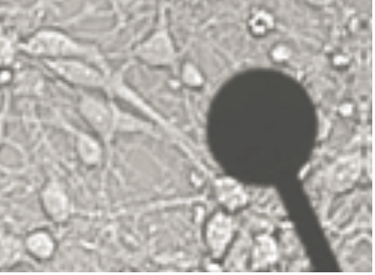
(a)

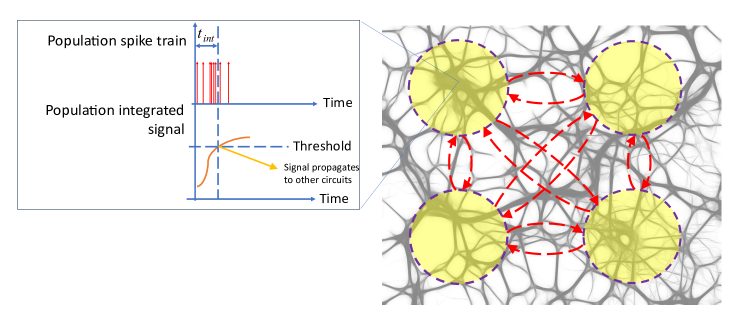
(b)

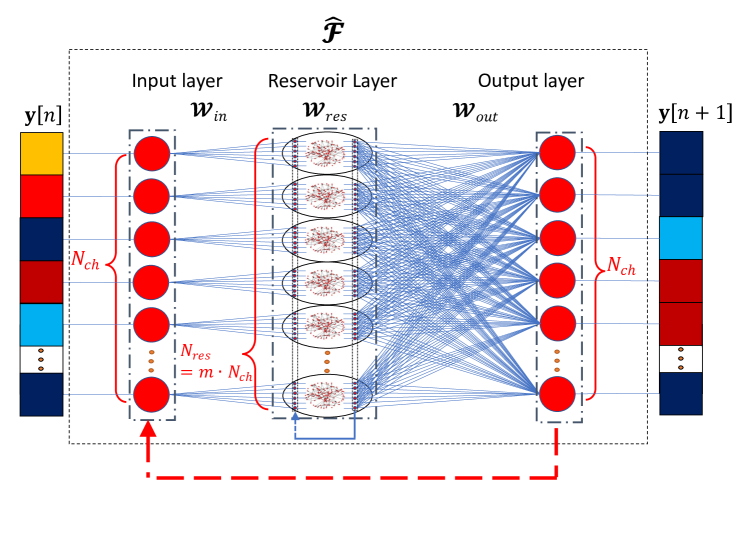
(c)

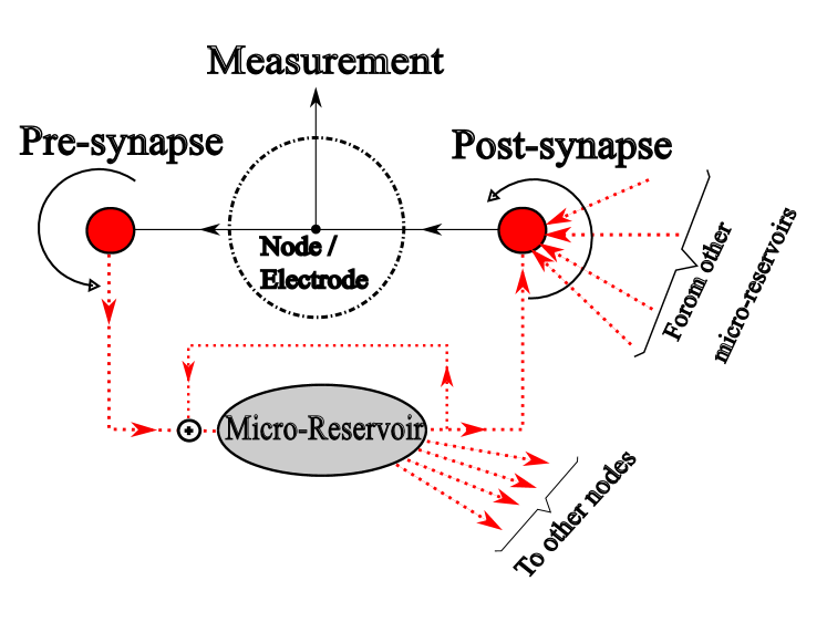
(d)

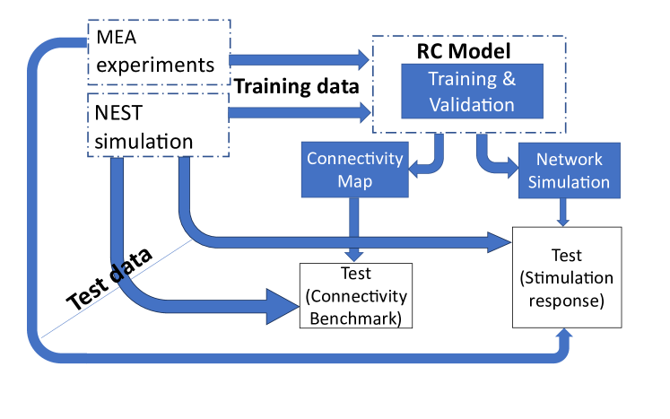
(e)

Figure 1: Description of the RC model. (a) A microscope image of microelectrode (diameter of 30 $\mu$m) surrounded by cultured neurons. This image illustrates how each electrophysiological measurement site samples signals from a complex circuit, whose morphology is not resolvable by simple methods. (b) An illustrative image of how the signals are intercepted by each electrode (yellow circles) from the biological neuronal network in the background. The spike trains collected at each electrode are then forming integrated signals which propagate within the network. (c) The artificial neural network (ANN) design of the RC model. Consists of three layers (input, reservoir, output) and a recurrent branch. It describes how the state of the network $\mathbf{y}$ (described by $N_{ch}$ samples of the measured signals) is processed from time step $n$ to time step $n+1$. (d) Enhanced visual representation illustrating the interconnection between the computational circuitry of the RC model and the intricate circuitry of biological signals. (e) A block diagram illustrating the sequential computational processes, including training, validation, and testing, conducted in this study.

Let us consider the training data matrix $\mathbf{Y}\in\mathbb{R}^{N_{ch}\times N_{t}}$ which governs $N_{t}$ time steps of the observed network state, i.e. $\mathbf{Y}=\Bigl{[}\mathbf{y}[1],\mathbf{y}[2]\ldots\mathbf{y}[N_{t}]\Bigr{]}$. The task of the training is to optimize output layer’s matrix weights $\mathcal{W}_{out}$ and biases $\mathbf{b}$, between each input-output pair $(\tilde{\mathbf{y}}[n],\tilde{\mathbf{y}}[n+1])$ (Eq. (2)) in order to minimize the error between $\mathbf{Y}$ and $\tilde{\mathbf{Y}}$. To achieve the optimization we use the Lasso regression method [14], with the loss function:

$$\mathcal{L}=\frac{1}{N_{ch}}\sum_{i=1}^{N_{ch}}\left\{\left\langle\left\|\tilde{y}_{i}[n]-y_{i}[n]\right\|^{2}\right\rangle_{n}+\lambda\sum_{j}\left|W_{out}^{i,j}\right|\right\}$$ (3a)

$$\tilde{y}_{i}[n]=\sum_{j}W_{out}^{i,j}\cdot x_{j}[n]+b_{i}$$ (3b)

where $\lambda$ is the lasso regularization parameter [14]; the $\langle\cdot\rangle_{n}$ notation indicates average along the time steps dimension. Then the regression objective is:

$$\left\{\mathcal{W}_{out},\mathbf{b}\right\}=\underset{{\mathbf{w},\mathbf{b}}}{\arg\min}\bigl{(}\mathcal{L}\bigr{)}$$ (4)

where $\mathbf{w}$ denotes all the weights in matrix $\mathcal{W}_{out}$. The lasso regression method was chosen due to its effectiveness in finding the lowest required weights, preventing them from exploding, as well as effectively omitting the unnecessary weights (setting them to zero).

2.2 Retrieval of Connectivity Map

Here we demonstrate the first feature of the discussed RC-based model, which is the ability to derive the connectivity map between the measurement sites from the spatio-temporal dynamics encoded in the electrophysiological signals. Connectivity refers to the weighted relationships between the different units of the network (single neurons, populations or circuits of any type). In this analysis, we assume that this nonlinear dynamic system, can be in principle separated to linear and nonlinear regimes. Let us assume that the training of the ANN has achieved sufficiently low loss score (Eq. (3)), indicating that the model has learnt sufficiently well the dynamics of the given network. Looking at the dynamics described by Eq.(2), we note that the network state $\mathbf{y}[n]$ evolves in such way that the hypothetical connection weights between the nodes of the network are excited or depressed according to the propagation of signals within it (similarly to a biological network). We assume, however, that these complex dynamics are founded on an intrinsic network, built of fundamental connections with nominal weights. These connections could be associated with the linear regime of the dynamics. Hence, we represent Eq.(2), describing the network state $\mathbf{y}[n]$ evolution, by the following discrete differential equation:

$$\mathbf{y}[n+1]=\mathcal{T}_{0}\mathbf{y}[n]+\mathcal{G}\Bigl{\{}\mathbf{y}[n],\mathbf{y}[n-1],\mathbf{y}[n-2]\ldots\Bigr{\}}$$ (5)

where $\mathcal{T}_{0}$ is defined as the Intrinsic connectivity matrix (ICM), describing the linear relation between consecutive states. $\mathcal{G}$ denotes a nonlinear transformation that captures higher-order interactions, embodying the memory of the network. By linearizing the dynamics, it yields that:

$$\mathcal{T}_{0}=\mathcal{W}_{out}\hat{\mathcal{S}}\mathcal{W}_{in}$$ (6)

This allows to depict the morphology of this network using a directed graph of nodes and edges. Each node represents a neuronal population, whereas the edges represent the connections, with its appointed weight, where a weight of a connection represents the coupling strength between the two populations. Fig. 2 shows an example of a connectivity map obtained by the RC model and compared to the ground truth map.

In this part of the work we show the validity of the predicted ICM to represent the actual connectivity between the nodes of the network, each representing a neuronal population. We compared this prediction by the RC model with the performance of other common methods, such as Cross-Correlogram (CC) [10, 11] and Transfer Entropy (TE) [12]. As a benchmark, we built a simulation of a neuronal network with ground-truth connections between the neurons. The network has been built and simulated on NEST simulator [13], where we created virtual array of electrodes which sampled the signals from a defined population of neurons, similarly to conditions found in an experimental electrophysiological recording, such as microelectrode array (MEA). We assessed prediction accuracy through two distinct methods: 1. Receiver Operating Characteristic (ROC) Curve Analysis: This method illustrates the model’s predictive performance in a binary context, distinguishing between the presence and absence of connections. We evaluated the performance with the Area Under Curve (AUC) of the ROC curve. 2. Pearson Correlation with Ground Truth: This metric offers a quantitative measure of prediction quality by not only capturing the presence or absence of connections but also quantifying the accuracy in predicting connection weights. These weights may encompass both excitatory (positive values) and inhibitory (negative values) connections within the network.

(a)

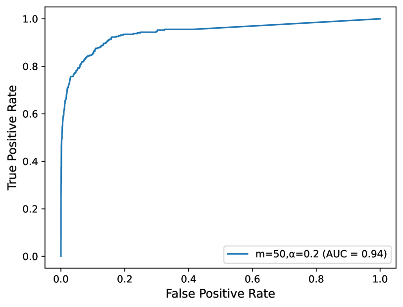
(b)

Figure 2: An example of connectivity map result obtained by the RC model. (a) A connectivity matrix and a connectivity graph map are presented for both the ground truth network (left hand side) and the connectivity map obtained by the RC model (right hand side). The Ground truth network was simulated on NEST simulator, producing electrophysiological activity which was then decoded by the RC model and obtaining the Intrinsic Connectivity Matrix (ICM). Note that the RC model predicted with a very high accuracy the existence of 3 uncoupled groups. In addition the model distinguished with a high accuracy between excitatory connections (positive weights) and inhibitory (negative weights). The nodes in the graphs represent neuronal population (or circuit) and the edges represent effective synaptic connections. The predicted map displays only weights with absolute values exceeding 0.1. (b) The corresponding ROC curve. In this example: $\rho=0.72$; $AUC=0.94$ for $\alpha=0.2$ and $m=50$.

We examined the model performance for different network configurations, such as the size of the network in terms of number of populations and the training data richness, which we defined as:

$$q\triangleq\frac{N_{t}}{N_{ch}}$$ (7)

$N_{t}$ is the total number of time steps used in the training and $N_{ch}$ is the number of populations equivalent to the number of channels in the experimental data. Fig. 3 summarizes the connectivity retrieval and validation results.

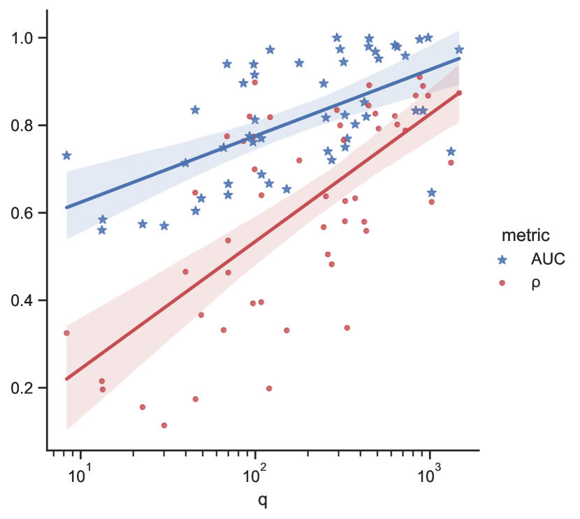
(a)

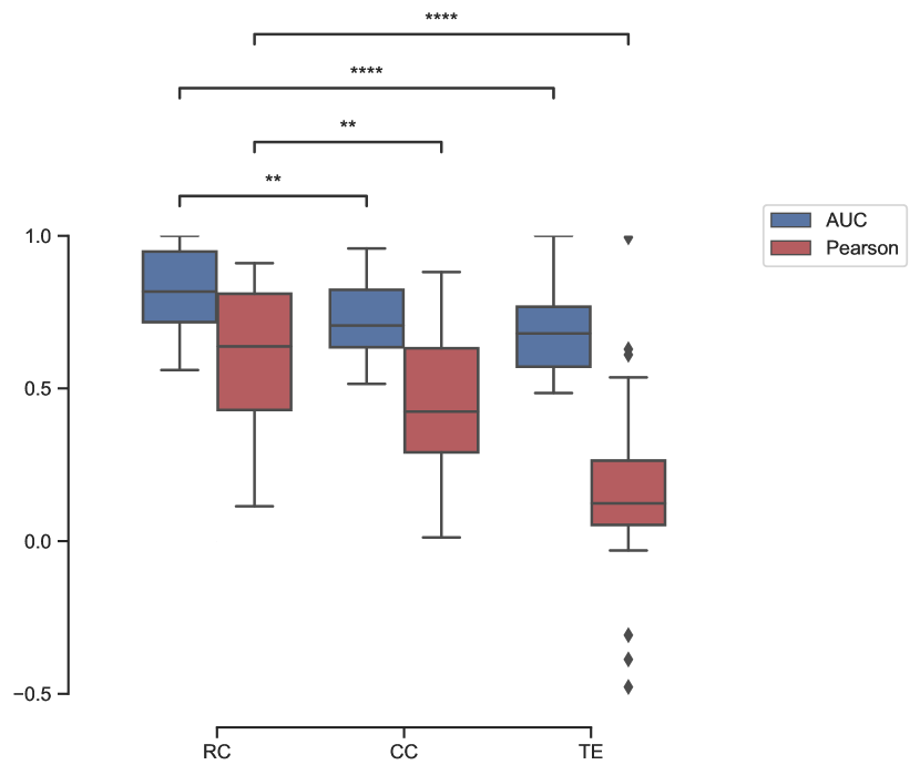
(b)

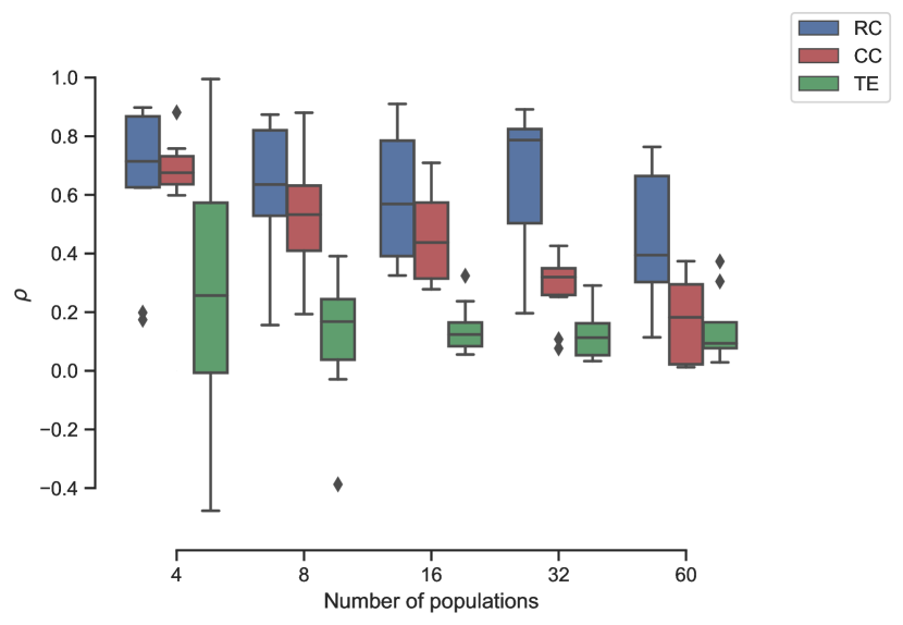
(c)

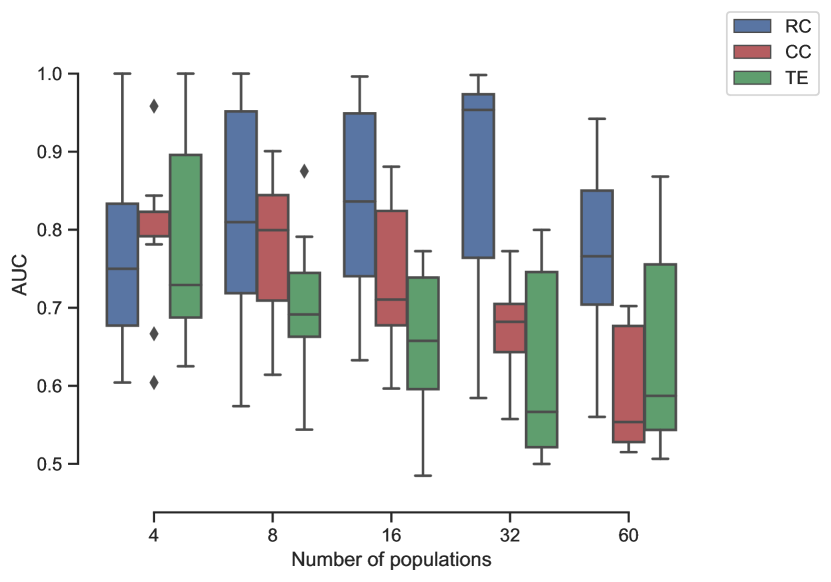
(d)

Figure 3: Connectivity retrieval performance. (a) RC model connectivity prediction accuracy in terms of Pearson correlation ($\rho$) and ROC AUC metrics as a function of $q$, a parameter representing the richness of the training data (Eq. (7)); (AUC: $R^{2}=0.38$), ($\rho$: $R^{2}=0.47$). (b) Comparison between the performances of different algorithms for connectivity prediction. RC model is compared to two other common methods for connectivity retrieval: Cross-Correlation (CC) and Transfer Entropy (TE). In this comparison two-sided Mann-Whitney-Wilcoxon test with Bonferroni correction was applied; AUC-RC vs. AUC-CC: $U-stat.=1820$, $p-value=4.527\times 10^{-3}$; $\rho$-RC vs. $\rho$-CC: $U-stat.=1864$, $p-value=1.568\times 10^{-3}$; AUC-RC vs. AUC-TE: $U-stat.=1993$, $p-value=4.402\times 10^{-5}$; $\rho$-RC vs. $\rho$-TE: $U-stat.=2417$, $p-value=2.534\times 10^{-12}$; (c),(d) Performance comparison between RC model, CC and TE categorized by the complexity of the network in terms of number of sampled populations, where each population represents a circuit of 5 neurons: Figure (c)- $\rho$ metric; Figure (d) AUC metric.

2.3 Prediction of spatio-temporal response of the network

The connectivity analysis discussed in the previous subsection provides mapping of the network intrinsic connections. Here we evaluate the performance of the model to predict the response of the network, given a specific input (stimulation).

Considering that the model has undergone training based on the inherent spontaneous activity within the network, capturing the fundamental signal propagation between populations in response to minor perturbations. Upon acquisition of a trained model (Eq. (3), (4)), from Eq. (2), we posses the following operator (synaptic function):

$$\tilde{\mathbf{y}}[n+1]=\hat{\mathcal{F}}\Bigl{\{}\tilde{\mathbf{y}}[n]\Bigr{\}}\$$ (8)

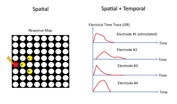
Figure 4: Illustration of the stimulus test designed to assess the RC model’s network response prediction performance to a local stimulus. On the left, an electrode map highlights the stimulated electrode (in red) and the responsive electrodes (in yellow), demonstrating spatial prediction. This is further evaluated against the experimental/simulated response using the ROC AUC metric. On the right, a detailed temporal response from all involved electrodes showcases spatio-temporal prediction. This is quantitatively compared to the experimental/simulation test using the $\bar{R}$ metric (refer to Eq. (9)).

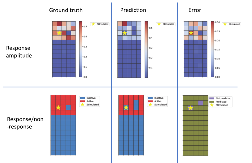
(a)

(b)

(c)

Figure 6: An example of a response test to a specific stimulation protocol (NEST simulation data). A stimulus was given around a neuronal population found on the third row and third column of the map (designated with a yellow star). (a) The ground truth response (simulated in NEST), Predicted response and the error between them. Two types of comparisons are shown- the prediction in terms of amplitude, for which the channel-wise error is given by $\varepsilon$ (Eq. (28); and a binarized prediction to distinguish between responsive and unresponsive channels, which further was analyzed using the ROC curve AUC. For this example: $AUC=1$ at $\alpha=0.5$ and $m=50$. (b) The corresponding ROC curve. (c) a detailed map of each channel’s response in a fixed window of time (full time axis = $40ms$, time step (integration time) = $2ms$). The $y$ axis is the normalized ISR in arbitrary units. $\bar{R}=0.158$ at $\alpha=0.5$ and $m=50$.

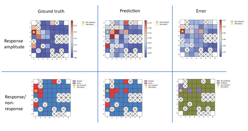
(a)

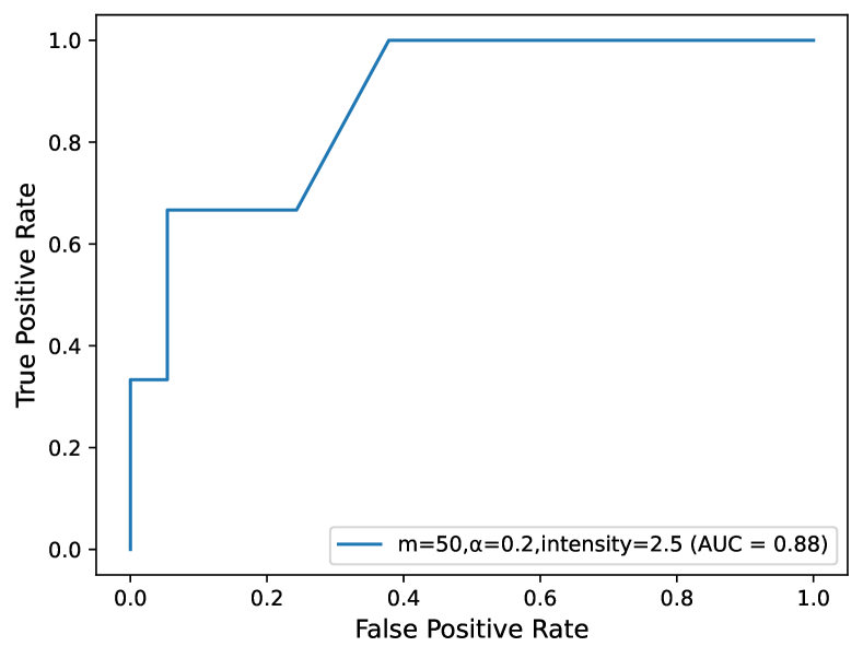
(b)

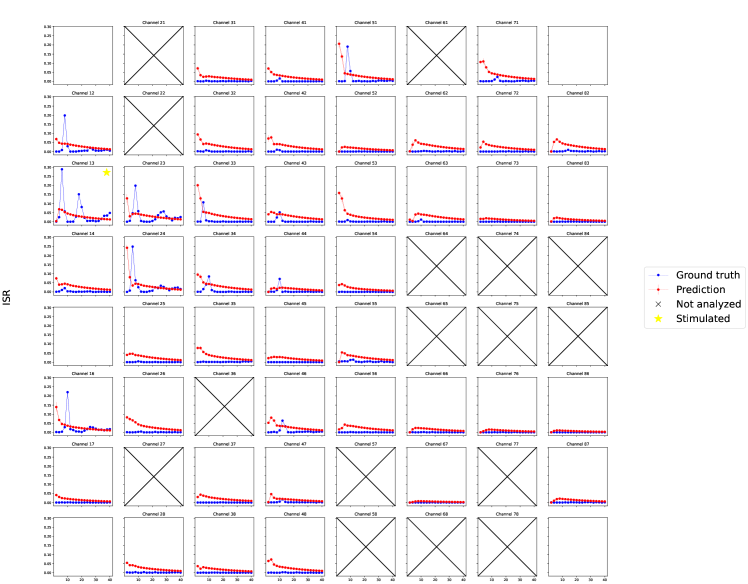
(c)

Figure 7: An example of a response test to a specific stimulation protocol (MEA experiment data). (a), (b) and (c) share the same description of Fig. 6. The X’s correspond to channels that were discarded from analysis due to low activity. $\bar{R}=0.047$; $AUC=0.87$ @$\alpha=0.2$ and $m=50$.

Hence, given an initial state $\tilde{\mathbf{u}}[0]=\mathbf{u}_{in}$, representing locally stimulated population, we obtain the predicted response of the network $\tilde{\mathbf{U}}$, by propagating the initial state for a number of time steps. For evaluating the prediction, we need to estimate the error between the predicted response $\tilde{\mathbf{U}}$ and the observed (ground truth) response $\mathbf{U}$. For this evaluation, we prepared a specific test data $\mathbf{U}$ for every tested neuronal network (experimental and simulated), corresponding to a localized stimulus applied in the vicinity of a specific neuronal circuit (in the experimental context- around a specific electrode).

In this context, we conducted a comprehensive evaluation of prediction quality through two distinct approaches: 1. ROC Curve Analysis: This method enabled us to spatially discriminate between responsive and unresponsive circuits. 2. Error evaluation between the full temporal profile of $\mathbf{U}$ and $\tilde{\mathbf{U}}$: To assess the predictive performance of temporal responses within network circuits, we introduced the following error function, based on the root-mean-squared-error (RMSE):

$$\bar{R}=\sum_{i}\chi_{i}\min_{\tau}\left(\sqrt{\sum_{j}\chi_{j}\bigl{(}U_{i,j}-\tilde{U}_{i,j-\tau}\bigr{)}^{2}}\right)$$ (9)

Where $\chi_{i,j}$ are the spatial and temporal weighting coefficients respectively; $\tau\in[\tau_{min},\tau_{max}]$ is the time lag between the predicted and the observed responses. This metric quantified the accuracy of our predictions in capturing both the amplitude and time lag aspects of the actual responses, providing a comprehensive evaluation of temporal prediction quality. Fig. 4 illustrates the concept of only spatial and spatio-temporal predictions. Figs. 6 and 7 show an example of the response prediction test of the RC model using electrophysiological data from NEST simulation and MEA experiment, respectively. Figs. 9 and 10 show the summary of the results for the response prediction test in terms of $\bar{R}$ and AUC metrics for electrophysiological data from NEST simulation and MEA experiment, respectively.

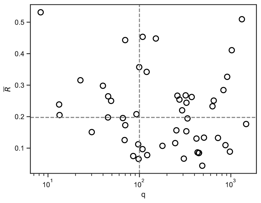
(a)

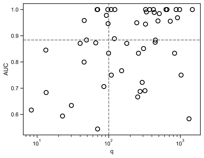
(b)

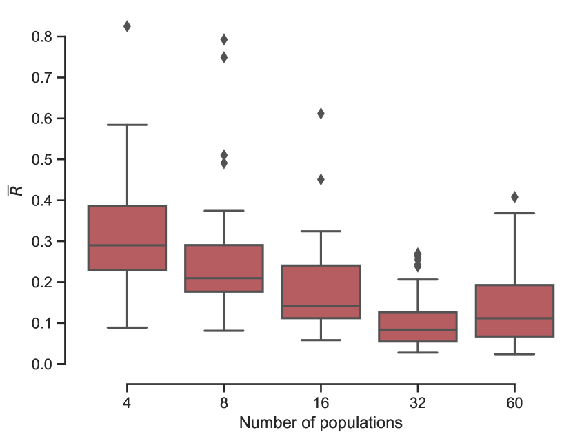
(c)

(d)

(e)

(f)

Figure 9: Performance of the RC model for the network response prediction (NEST simulation data). The RC model underwent training using the basal activity of a specific network. Subsequently, the trained model was subjected to testing through local stimulation, and its response was compared against the corresponding ground truth response, as simulated in NEST. (a), (c) and (e) present the $\bar{R}$ metric (spatio-temporal response)- lower values are indicative of a more accurate prediction; (b), (d) and (f)- AUC metric (spatial response)- values closer to 1 indicate more accurate prediction. (a), (b) the metrics as a function of $q$ (Eq. (7)) the horizontal dashed line indicates the median value of the associated metric, the vertical line is at $q=100$, which we set as an arbitrary boundary between sparse and dense data. Each dot corresponds to the mean metric per experiment of a specific network (averaged over different stimulation protocols). It is noteworthy that denser datasets, characterized by large values of $q$, generally yield more accurate prediction outcomes. (c), (d) box plots of the metrics categorized by the simulated network size. (e), (f) the response test results plotted against the connectivity results of the corresponding network. A noticeable correlation between the two is observed ($\bar{R}$ vs. $\rho$: $R^{2}=0.060$; Response AUC vs CM AUC: $R^{2}=0.176$)

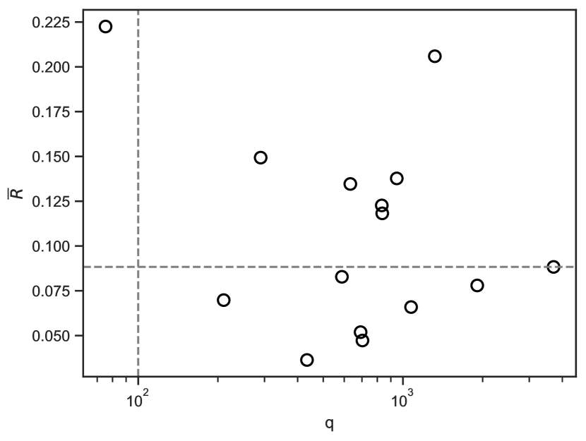
(a)

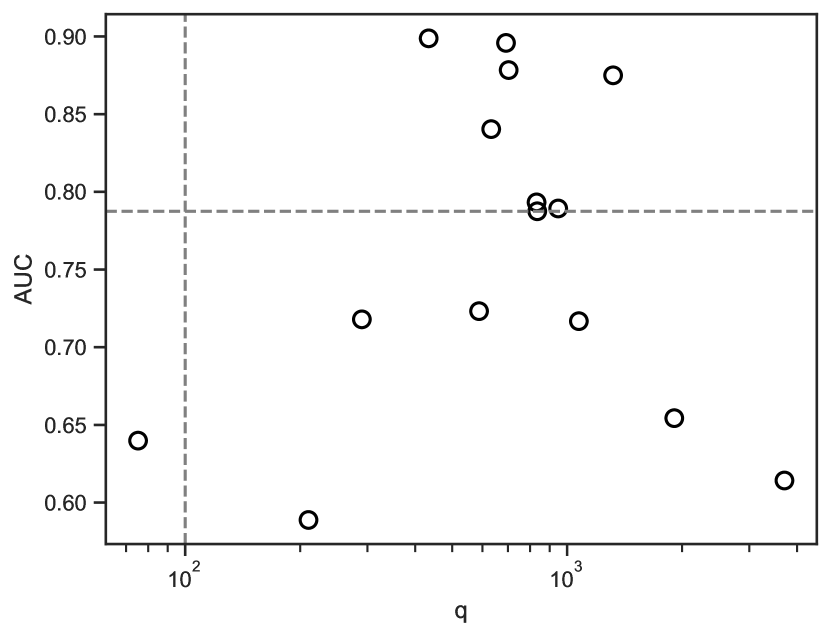
(b)

Figure 10: Performance of the RC model for the network response prediction (MEA experiments data). (a) and (b) share the same description of Figs. 8(a), 8(b).

Table 1: Summary of the response prediction test by the RC model. The table shows the results concerning the 2 metrics used: $\bar{R}$ (spatio-temporal prediction) and AUC (spatial prediction). The datasets originate from both NEST simulations and MEA experiments.

Data type	# Protocols (out of # experiments)	Metric [mean $\pm$ std]
		$\overline{R}$	$AUC$
NEST Simulation	183 (51)	$0.195\pm 0.141$	$0.876\pm 0.222$
MEA Experiment	27 (15)	$0.104\pm 0.054$	$0.754\pm 0.160$

3 Discussion

In this work we developed a computational model which decodes spatio-temporal data from electro-physiological measurements of neuronal cultures, reconstructs the network structure on a macroscopic domain and can predict the response of a given network. The main aim of the model is to create an advanced experimental data analysis tool for processing complex time-series. The results obtained indicate that the model functions not just as a data analyzer but could also be used as a network simulator. Below we review the fundamentals of the model, we also attempt to give interpretation to the computational processes and we openly address some of the limitations we have encountered during our research.

The main idea on which the model has been developed relies primarily on the neural rate-coding of information paradigm [15], which states that firing rate (of action potentials) is the main carrier of information in the communication between the neuronal cells. The second presumption that establishes the model regards the essence of electrophysiological measurement of large neuronal populations, in particular extracellular measurements, which have been used to validate the model. As for the computational structure, the model is founded on a recurrent neural network (RNN) with RCN architecture. The rationale to use this kind of neural network for the current motives is rather self-evident. It has been shown in various studies that biological neuronal networks (e.g., the brain cortex) possess complex computational capacities, in particular temporal data is integrated in a recurrent manner and induce state-dependent synaptic transmission [16, 17, 18, 19, 20]. In other words, the network memorizes the previous impulses and modifies its synapses accordingly. The time-scale of this process varies according to the functionality of the network. RCN is a bio-inspired approach, where the neural recurrence and nonlinearity are taken into account. Another great advantage of this approach is the simplicity of the training, where only the output layer is trainable. The output layer can in principle be fully linear (but not necessarily), as the nonlinearity is embedded in the reservoir neurons. Utilizing a linear output layer gives the possibility to train the network with linear regression, which makes the process significantly cheaper (in terms of computational power) than training multilayered recurrent neural networks, such as Long-Short-Term-Memory (LSTM).

RCN has been used in studies of electrophysiological signals from neuronal networks, in particular in these works the guiding principle is the exploitation of the reservoir-like properties of neuronal networks to adapt it to perform input-output tasks [8, 21, 7, 22, 23]. Our methodology, on the other hand, is to simulate the neuronal network using RCN approach to extract the network properties of a given culture such as the connectivity map of the network and its functionality on a macroscopic scale. Similar attitude towards this question was reported in [24] where the RCN approach was applied to learn the dynamics of spike-trains in neuronal cultures, in particular in MEA recordings. The work however focused on the prediction of spike-trains as a point-process propagation between distinctive input and output nodes, using the log-likelihood optimization. Additionally in that work, the authors implemented different types of neural networks, including an adaptive reservoir with a nonlinear output layer, which in practice transcends the modeling complexity discussed in this paper.

In this work, we implement RCN as rate-coded spiking neural network, which we train to adapt the time-domain nonlinear synaptic function. The data that is used to train the model is rate-encoded spike trains. This data structure follows an assumption that the spikes that propagate within the network carry information in a characteristic time constant window (unique to each network) and is defined as the spike-integration time. In addition, we extract from the data, temporal events that exhibit significant spiking activity in short period of times (network bursts). As a result the time-series data undergoes a significant dimensionality reduction.

The unique RCN design we have implemented decompose the information processing of the network at each time step (lasting one integration time in the real-world) to a pre-synaptic stage, executed by the input layer and the input of the reservoir layer; and the post-synaptic stage executed by the output layer and the output of the reservoir layer (Figs. 1(c),1(d)). This stage sequence correspond to one time-step and does not necessarily describe the realistic temporal propagation of signals within this time window. The reservoir layer consists of a number of independent micro-reservoirs which is equal to the number of the macroscopic network nodes (corresponding to the number of measurement sites or electrodes). In the pre-synaptic stage we sample the network state, each node independently by its own micro-reservoir. Each micro-reservoir integrates its current state with the input signal and applies nonlinear function. In the post-synaptic stage, the integrated and processed state of the reservoir (which is composed of all micro-reservoir states), is linearly mapped to the next network state, taking in consideration the synaptic coupling between the different micro-circuits.

The model, to some extent, is founded on the nonlinear leaky integrate-and-fire approach [5]. The structural design of our Reservoir Computing Network (RCN) adheres to distinct principles governing energy dynamics within the network. At its core, the structure is built upon the fundamental principles of reciprocity and energy conservation, augmented by the incorporation of a leaky memory and nonlinear elements. The dynamic behavior is intricately described through the interplay of information integration and synaptic energy exchange.

We showed that by adapting the model to produce the dynamics observed in the experiments followed by applying a linear approximation of the transfer function, we obtain the fundamental (or intrinsic) connections between the populations of the network. These intrinsic connections describe the fundamental connectivity of the given network without internal or external stimuli that may modify them. Indeed, as seen from the equations describing the dynamics, during the full operation of the model these connections change depending on the activity of the network. The connectivity map we obtain from this analysis can be referred as Effective Connectivity rather than Functional Connectivity [25], because the resulting connections are derived from the actual causality relations between the populations based on the electrical signals; in contrast to the statistical relations seen in Cross-Correlation or Transfer Entropy analysis, which yield connectivity referred as Functional Connectivity and hence we assess the better performance of this model in predicting the connectivity of the network.

Further, we tested the predictive capabilities of the model in terms of input-output prediction. Here we trained the model on the network basal (spontaneous) activity, with the assumption that this dataset would unveil the interactions among network nodes. During the testing phase, we posited that applying local stimulation to the network would elicit a correlated response from the circuits connected to the stimulated population. To assess this hypothesis, we gathered distinct datasets: one capturing spontaneous activity and another capturing evoked activity resulting from a local stimulus. The former was employed for training and validation, while the latter served as the test dataset. We subsequently simulated the model’s response to the specific stimulus and assessed the accuracy of our predictions. This procedure was carried out using both synthetic and experimental data. With ROC curve metrics, we have found that the model can spatially predict with high accuracy the network nodes that respond to the stimulus. However we also tested how accurate the prediction is in the temporal window of each node (electrode). Here we have found that the temporal profile of the predicted response may be distorted or time shifted. This could be due to the fact that some physical attributes of the stimulus are not taken into consideration of this model, such as the stimulus pulse shape (in amplitude and time) and hence the temporal dynamics is limited to time scales of the discretized time-step (defined as the integration time), nevertheless the temporal prediction in some cases reached high performance. The limitations in achieving precise temporal predictions may not solely be attributed to the model’s constraints, but also to the chosen training approach. For instance, the simplifying assumption that predicting evoked activity can be accomplished solely by learning from basal activity might prove to be overly simplistic. Nevertheless, the model is not confined to the specific training and testing approach involving spontaneous and evoked activities. In practical applications, any type of electrophysiological signal data, following the same data collection principles, can be employed to train the model and potentially improve its prediction abilities. For example, utilizing the evoked activity dataset can reveal the connections within the circuitry responsible for responding to the stimulus.

As one would expect, the performance of the model is directly dependent on the data it is trained on. An important (but may not be sufficient) feature in the data is its spiking modality. The spiking data is expected to be modulated in such way that there should be a typical or a range of time that the network exhibits fast spiking events at numerous channels. These events are often seen as synchronous or quasi-synchronous [26, 27]. In this way, the data can be easily separated to temporal windows of these time events, while the silent phases are discarded. Each of these windows serve as data batch. This quality can be seen in the inter-spike interval (ISI) histogram, where a bimodal (or multi-modal) shape presents. Another element in the data, which affects the quality of the model performance is the presence of the causality between time-steps, discretized by a typical short-time window (time-bin), which we infer as the spike integration time of each circuit. The model in fact is trained to find this causality between the time-steps, and as the integration time is, in principle, a free parameter, we have found that the performance of the model is strongly dependent on this value. This implies that the network has a characteristic time constant (or quasi-constant) that defines its information processing time. We assume that this integration time, can be obtained from some attributes of the data. We have found that the most significant peak of inter-burst-interval (IBI), can serve as a good approximate of this value (see supplementary materials). This feature is also related to the stochasticity of the data, since it can determine the ability of the model to learn the spatio-temporal patterns. The characterization of the data degree of stochasticity is beyond the scope of this paper.

Another limitation which we discuss here is the fact that biological systems can exhibit modifications in their structure in rather short times. Since the data analysed by the discussed model describe the setting of the tested culture within a limited time frame, it is possible that some information about the tested culture can be missed. Therefore for using this model for systems that may vary fastly in time, it is possible to apply the training for short time sessions, and eventually to see the development of the system.

In summary, we have developed a computational model which is based on RCN. The model decodes the spatio-temporal patterns of spike-data and reconstructs the connectivity map of the tested network. The model is also used to predict the response of the given network to local stimuli. In this paper we developed and tested the model on data from in-vitro neuronal electrophysiological signals recorded on 60 electrodes MEA. In-vitro studies of neurons give a simplified representation of the structure and functionality of these networks in living organisms [28, 29]. Such approach assists in decomposing the extremely complex structure of living brain into smaller functional blocks. We assess that the methodology developed in this work can be also applicable on data with higher spatial resolution (such as from HD-MEA [30]) and hence to give - up to interactions between single neurons. In addition the model is not restricted to analyze only neuronal signals, but can also be applied on different types of time traces.

4 Methods

4.1 The paradigm

We consider a multi-site measurement of electrophysiological signals from a neuronal culture, such as 2D microelectrode array (MEA). We seek to represent the tested culture as a network where each node corresponds to one measurement electrode. Each electrode samples the electrophysiological signals from the neuron ensemble (consisting of a few neurons) found in its vicinity (Fig. 1(a)). Therefore, each node has to represent a complex neuronal circuit whose dynamics by itself is driven by numerous interacting neurons. We hence define the domain of the measurement as the macroscopic domain, which is described by the network in question; whereas the neuronal structure sampled by each node will be referred as the microscopic domain (or later as the reservoir domain). The data unit which is contained in each of these nodes is a sample of the electrophysiological signals expressed in instantaneous spike-rate measured in a specified time window. By “data unit” we refer to a set of data sampled at the network nodes in a definite time window, which contains information on the status of the network, with a memory on the previous time steps, and the ability to predict the next step accordingly. The time window is determined by a characteristic information flow rate of the network. This unit of time is dependent on many properties of the network such as neuron density in the culture, age of the culture and other [26], and it characterizes the signal integration time of each node.

Let us represent the macro-domain state of the network at each time step $n=1,2,3...$ with a vector $\mathbf{y}[n]$, where each component of the vector describes the state of a single node, i.e., $\mathbf{y}[n]$ is the signal representation of each electrode at time $n$. Our aim is to seek the time propagation operator (or a synaptic transmission function) $\hat{\mathcal{F}}$ (Eq. (8)) transforming state $\mathbf{y}[n]$ to $\mathbf{y}[n+1]$. The operator $\hat{\mathcal{F}}$, which is likely to be non-linear due to the nature of neuronal networks, should describe as closely as possible the experimental observation in the electrophysiological measurements, i.e., we aim to fit a model to an observation which can mimic or predict the spatio-temporal patterns of the neuronal activity in the culture under test.

We then consider the fact that each node in the macro-domain network represents a complex neuronal signal-processing-unit. It arises from the fact that typically every measurement site is surrounded by neurons which may be as many as a dozen. The morphology and functionality of each of these micro-circuits embedded in each node of the macro-domain network cannot be easily obtained from the electrophysiological measurements of standard recording systems. Also modeling of such neuronal structures is not an easy task and has been studied for decades, with numerous models for different scales of dimensions and time [4, 5].

Hence our approach is to represent each measurement node (electrode) as a gate to a particular neuronal circuit (reservoir), where the signals measured at each node are an outcome of a complex operation involving each circuit and the whole network. We therefore propose the artificial neural network (ANN) structure depicted in Fig. 1(c) This structure represents a simplification of the neuronal dynamics, where each of the neuronal circuits is a black box, whose morphology and functionality are not known but assumed to be reasonably random.

As seen in Fig. 1(c) and 1(d), we assume that the signal sampled at each node is an input to and an output from a higher dimensional domain with a specific connectivity and functionality. At the input of the ANN, the signal at each node is transformed to a corresponding reservoir-state (in the reservoir domain) by a set of uncoupled weighted connections (Input layer). Each micro-reservoir, associated with a node in the macro-domain, represents a micro-neuronal circuit embedded at each of the measurement sites, and has inner interconnections which represent the connectivity of the micro-circuits (Reservoir Layer). Each such circuit performs a nonlinear transformation, creating an updated reservoir state, which on one side is stored as a memory to be integrated to the next time steps, and on the other side is used to form the next state of the macro-domain network by weighting and coupling all the micro-reservoir states (Output Layer); then the whole process repeats cyclically. This kind of recurrent network is known as Reservoir Computing Network (RCN) and has been widely studied.

4.2 Artificial Neural Network Design

4.2.1 Domains and Dimensions

As mentioned above, the model distinguishes between two domains: The macro-domain which refers to the experimental observations, represented by the corresponding network; and the micro- (or reservoir) domain which refers to the neuronal units embedded in each of the macro network nodes, with no experimental data. We denote by $N_{ch}$ the dimension of the macro-network which in fact represents the number of nodes in the network, where each node is directly associated with an electrode (or a channel) in the experimental measurement. $N_{res}$ is the dimension of the reservoir.

Assuming that the neurons are uniformly distributed in the culture, we appoint a fixed number of connections between each node and the corresponding micro-circuit, such that for each node of the network there is one micro-reservoir (see Fig. 1(c)):

$$N_{res}=mN_{ch}$$ (10)

where $m$ is an integer number. It follows that each $m$ components in the vector space of the reservoir domain correspond to one node in the macro domain. In fact, we may associate $m$ with a relative size of each micro-circuit.

4.2.2 Input Layer

The input layer refers to the stage between the macro domain and the reservoir one. Here we assume that the data at each of the nodes is a linear transformation of the corresponding input state to the reservoir, such that each component in the macro-domain transforms directly to corresponding $m$ inputs of $N_{res}$ components in the reservoir domain, and refer to a single micro-circuit. This is done with the linear transformation described by Eq. (2a), where the state $\mathbf{y}\in\mathbb{R}^{N_{ch}\times 1}$ is transformed to the input reservoir state $\mathbf{x}_{in}\in\mathbb{R}^{N_{res}}$ through an input matrix $\mathcal{W}_{in}\in\mathbb{R}^{N_{res}\times N_{ch}}$. Since $\mathcal{W}_{in}$ maps each node to a corresponding micro-reservoir, it is represented by the following matrix:

$${\mathcal{W}_{in}=\begin{bmatrix}\left(\mathbf{w}_{in}^{(1)}\right)\par&0&0&\cdots&0\\ 0&\left(\mathbf{w}_{in}^{(2)}\right)&0&\cdots&0\\ 0&0&\left(\mathbf{w}_{in}^{(3)}\right)&\cdots&0\\ \vdots&\vdots&\vdots&\ddots&\\ 0&0&0&&\left(\mathbf{w}_{in}^{{(N_{ch})}}\right)\end{bmatrix}}$$ (11)

where each $\mathbf{w}_{in}^{(i)}\in\mathbb{R}^{m\times 1}$, $i=1,2,...,N_{ch}$ is a vector with random weights taken from a Normal distribution (peaked at 0), normalized such that $\|\mathbf{w}_{in}^{(i)}\|^{2}=1$, which can also be expressed as:

$$\mathcal{W}_{in}^{T}\mathcal{W}_{in}=\mathcal{I}_{N_{ch}}$$ (12)

where $\mathcal{W}_{in}^{T}$ is the transposed input matrix and $\mathcal{I}_{N_{ch}}$ is the unit matrix of order $N_{ch}$.

4.2.3 Reservoir Layer

The reservoir layer contains $N_{ch}$ independent micro-circuits with $m$ nodes each (total $N_{res}=m\times N_{ch}$ nodes). Each such circuit models the neuronal circuit around each electrode. This layer has two main functionalities: 1. nonlinear time-operator. 2. Reservoir state integrator. The dynamics of the reservoir layer is recurrent, where each time step $n$ the reservoir state $\mathbf{x}[n-1]$ is nonlinearly mapped into a new reservoir state $\mathbf{x}[n]$ (Eq. (2b)). This discrete differential relation provides cumulative data at each time step and carries the temporal memory on the activity of the network. Note that at time step $n$, the reservoir state $\mathbf{x}[n-1]$ undergoes an inner transformation through the reservoir matrix $\mathcal{W}_{res}\in\mathbb{R}^{N_{res}\times N_{res}}$, then integrated with the reservoir input state $\mathbf{x}_{in}$, followed by a nonlinear operation $\mathbf{f}_{NL}$. The operation of $\mathcal{W}_{res}$ is linear and describes the inner data propagation between the nodes of the reservoir. The synaptic morphology of each micro-reservoir is random and since they are independent, there are no coupling elements between them at this stage of the ANN. In addition, we assume that $\mathcal{W}_{res}$ preserves the energy of the state, hence it is represented by a block-diagonal and orthogonal matrix as the following:

$$\mathcal{W}_{res}=\begin{bmatrix}\left(\mathbf{W}_{res}^{(1)}\right)&0&\cdots&0\\ 0&\left(\mathbf{W}_{res}^{(2)}\right)&\cdots&0\\ \vdots&\vdots&\ddots&\\ 0&0&&\left(\mathbf{W}_{res}^{(N_{ch})}\right)\end{bmatrix}$$ (13)

where each $\mathbf{W}_{res}^{(i)}\in\mathbb{R}^{m\times m},i=1,2...N_{ch}$ is a random-orthogonal matrix. Note that each block acts on its corresponding micro-reservoir state.

Further we note in Eq. (2b) the memory parameter $0<\alpha<1$, which factorizes the orthogonal matrix $\mathcal{W}_{res}$. This represent the memory strength, such that the effect of the reservoir state $\mathbf{x}[n]$ on the state $\mathbf{x}[n+k]$ will scale as $\alpha^{k}$. $\alpha=0$ indicates that the system is memoryless and the current state at time step $n$ depends only on the input.

The nonlinear function $\mathbf{f}_{NL}$ in Eq. (2b) accounts for the impact of network saturation and plasticity. Specifically, when subjected to a persistent input, the reservoir tends to saturate, while in the absence of input, it retains an excited state due to the influence of preceding signals (plasticity). Note that the length of the plasticity effect depends on the parameter $\alpha$. In this work we tried to implement different types of nonlinear functions with such effects, such as tanh and sigmoid, however the performance of the model showed a weak dependence on the choice of the function. For the results presented in this paper we considered:

$$\mathbf{f}_{NL}(\mathbf{\xi})=\Theta(\mathbf{\xi})\tanh(\mathbf{\xi})$$ (14)

where $\Theta(\mathbf{\xi})$ is the $0$ / $1$ step function at $\mathbf{\xi}=0$ used to limit the emerging values from the reservoir layer to non-negative only. Further we note that in Eq. (2b) the nonlinear function is $\mathbf{f}_{NL}(\hat{\mathcal{S}}\mathbf{\xi})$. The factor $\hat{\mathcal{S}}$ gives each reservoir neuron a different strength of the nonlinear response. This operation does not couple the different neurons and hence $\hat{\mathcal{S}}\in\mathbb{R}^{N_{res}\times N_{res}}$ is represented by a diagonal matrix containing normally-distributed synaptic strengths on its diagonal.

4.2.4 Output Layer

The output layer transforms the reservoir state back to the macroscopic domain. Here we assume a fully connected layer, such that all the $N_{res}$ reservoir nodes are weighted and connected to $N_{ch}$ nodes of the macroscopic network. This layer practically expresses the synaptic connectivity between the different nodes of the network. It is assumed that this transformation is purely linear, taking in consideration that the overall nonlinearity of the model is dominated by the reservoir layer. The relation of the output layer is given by Eq. (2c).

Unlike $\mathcal{W}_{in}$, $\mathcal{W}_{res}$ and $\hat{\mathcal{S}}$, which are matrices with random and constrained weights, $\mathcal{W}_{out}$ has no constraints on the values of its weights, rather it is the layer which is trained with Lasso regression (Eq. (3)).

4.3 Data

The model operates on the principles of a rate-coded spiking neural network. For model training, we generated tailored datasets that govern episodes of network bursting (NB) activity, representing them as multidimensional sequences of ISR data. The data in this study were generated through either experimental in-vitro measurements, involving the recording of neuronal electrical activity using a 60-channel MEA, or through in-silico simulations using the NEST simulator. Both datasets underwent a similar preprocessing approach, where only significant culture activity was incorporated into the training dataset. This involved the application of burst and NB detection algorithms [31, 32]. The experimental dataset required additional preprocessing before burst detection, entailing the transformation of raw electrical signals into spike trains using filtering and a spike detection algorithm [33]. A comprehensive description of the experimental procedures and the algorithms employed in this study can be accessed in the Supplementary Materials section. Additionally, details regarding the in-silico simulation are provided in Section 4.6.

4.3.1 Circuit Integration Time and Data Binning

A fundamental principle underpinning the RC model is the utilization of rate coding for the transmission of neural information. Consequently, the training data was structured as a time sequence representing the network state, encoded in spike-rate values. This approach was based on the assumption that there exists a characteristic range of neural spike integration time (found to be within a timescale of a few milliseconds), defining the information processing duration for individual circuits or populations within the system. We empirically demonstrated a close correspondence between the integration time (yielding optimal performance of the RC model) and the peak of the inter-burst-interval (IBI) histogram within the 1-10 millisecond range. This IBI histogram was constructed using intervals between consecutive bursts across all channels, employing the procedure described in the Supplementary Materials, also used for the inter-spike-interval (ISI) histogram. The spike traces are subsequently segmented into time bins of width corresponding to integration time, where each bin contains the ISR. Accordingly, we transform the spike trains data to ISR data:

$$\mathbf{D}[i,t]\rightarrow\mathbf{\Sigma}[i,n]$$ (15)

$\mathbf{D}$ and $\mathbf{\Sigma}$ represent 2D matrices, where the first dimension under index $i$ denotes the channel number, and the second dimension represents the time domain. Specifically, $\mathbf{D}$ serves as the complete spike train dataset, containing firing times denoted as $t_{f}$:

$$\mathbf{D}[i,t]=\sum_{f}\delta(t-t_{i,f})$$ (16)

$\mathbf{\Sigma}$ is the time-binned spikes matrix, where $n$ serves as the bin index, later identified as the unit time step:

$$\mathbf{\Sigma}[i,n]=\frac{1}{t_{int}}\sum_{t=t_{n-1}}^{t_{n}}\mathbf{D}[i,t],\;\;t_{n}=n\cdot t_{int}$$ (17)

$t_{int}$ is the integration time (Eq. (1))

4.3.2 Training and Validation Datasets

Following the steps described in the previous subsection, we generate the training and validation datasets. To ensure a consistent domain for the RC model across all datasets, we standardize the ISR data within the $\mathbf{\Sigma}$ matrix, scaling its values to fall within the range of 0 to 1. Subsequently, we construct the dataset by extracting data batches from $\mathbf{\Sigma}$ in segments from the full-length data, employing the following approach:

$$\overline{\mathbf{\Sigma}}\Bigl{[}i,n_{j}:n_{j}+N_{j}+\Delta-1\Bigr{]}\rightarrow\mathbf{Y}_{j}\left[i,1:L_{NB}^{j}+\Delta\right]$$ (18)

$\overline{\mathbf{\Sigma}}$ is the normalized $\mathbf{\Sigma}$ matrix; $n_{j}$ refers to the time-bin which indicates the beginning of the $j$th NB. $N_{j}$ denotes the duration of the $j$th NB, specified in the number of time bins. The parameter $\Delta$ is used to accommodate extra time steps, guaranteeing the inclusion of the latter part of the NB. Accordingly, the matrix $\mathbf{Y}_{j}$ represents the training batch number $j$.

Subsequently, we distribute the batches in a shuffled manner, allocating 85% of them for training and reserving the remaining 15% for validation, creating matrices $\mathbf{Y}^{tr}_{j}$, $\mathbf{Y}^{val}_{k}$ accordingly.

All batches $\mathbf{Y}^{tr}_{j}$ are then provided to the lasso regression algorithm (Eq. (3)) as merged sequence $\mathbf{Y}^{tr}$ (merging all matrices $\mathbf{Y}^{tr}_{j}$ along time dimension). The training however is informed about a beginning of a new batch, by resetting the time step to $n=0$ and the resrevoir state to $\mathbf{x}[0]=0$ (Eq. (2b)); in such way we decouple effects of one NB on another, taking in consideration that the time interval between different NBs is considerably longer than the interaction between the populations. The remaining validation batches $\mathbf{Y}^{val}$ are then used to evaluate the training, by calculating the validation loss:

$$\mathcal{L}^{val}=\frac{1}{N_{ch}}\sum_{i=1}^{N_{ch}}\ell_{i}$$ (19a)

$$\ell_{i}=\sqrt{\sum_{n}\omega_{i}[n]\left|\tilde{y}_{i}^{val}[n]-y_{i}[n]\right|^{2}}$$ (19b)

$$\tilde{y}_{i}^{val}[n]=\sum_{j}\bar{W}_{out}^{i,j}\cdot x_{j}[n]+\bar{b}_{i}$$ (19c)

$$\omega_{i}[n]=\left\lvert\frac{y_{i}^{val}[n]+\tilde{y}_{i}^{val}[n]}{\sum_{n}(y_{i}^{val}[n]+\tilde{y}_{i}^{val}[n])}\right\rvert$$ (19d)

$y_{i}^{val},\tilde{y}_{i}^{val}$ are the ground truth and modeled validation data for each channel $i$; $\bar{W}_{out},\bar{b}$ (Eq. (19c)) are the trained weights of the output matrix $\mathcal{W}_{out}$ and bias vector $\mathbf{b}$ (Eq. (3)); To enhance the robustness of our predictions, we address the issue arising from a significant portion of zero sequences in the traces $y,\tilde{y}$. The prevalence of these zero sequences can potentially lead to overly simplistic predictions. To mitigate this, we incorporate weights $\omega$ (Eq. (19b)) into our loss estimations. These weights, defined in Eq. (19d), are designed to assign greater importance to non-zero predictions within the trace, thereby addressing the potential bias introduced by the prevalence of zero sequences and enhancing the sensitivity of the model to more informative elements in the data.

4.4 Linearized Model and Connectivity Analysis

Let us observe the dynamics of the model. If the initial state of the reservoir is $\mathbf{x}[0]=0$ (unexcited state), we note that, without any input $\mathbf{y}$, the time sequence of the reservoir state, $\mathbf{x}[n]$, (2b), will not change its state and as a consequence, according to (2), no dynamics in the network nodes $\mathbf{y}[n]$ will be observed. Let us assume (without the loss of generality) that at a certain time-step $n=1$ we have a small perturbation, $\mathbf{y}[1]$, such that according to (2b) the following holds:

$$\mathbf{x}[1]=\mathbf{f}_{NL}\left(\hat{\mathcal{S}}{\mathcal{W}_{in}\mathbf{y}[1]}\right)\approx\hat{\mathcal{S}}{\mathcal{W}_{in}\mathbf{y}[1]}$$ (20)

This approximation is valid for any nonlinear function that satisfy $f(\xi)\approx\xi$ for $\xi\ll 1$, e.g., (14). If such linear regime is maintained in the following $k-1$ steps, from (2) it yields that the network output at time step $k+1$ is:

$$\mathbf{y}[k+1]\approx\sum_{n=1}^{k}\alpha^{n-1}\cdot\left[{\mathcal{T}}_{n-1}\right]\>\mathbf{y}[k-n+1]$$ (21)

where,

$$\mathcal{T}_{p}=\mathcal{W}_{out}\hat{\mathcal{S}}\left[\mathcal{W}_{res}\hat{\mathcal{S}}\right]^{p}\mathcal{W}_{in}$$ (22)

is a $N_{ch}\times N_{ch}$ transfer matrix of order $p$ (note that we omitted the constant bias vector $\mathbf{b}$ from (2c), since it describes a constant DC offset, and as known a posteriori, its value is small).

Assuming that the regression (Eqs. (3),(4)) as part of the model training has achieved low training and validation error score, means that a feasible parametrization for the equations of the nonlinear model (2) has been found. It follows that the transfer matrices (22) contain the connectivity weights between the nodes in the linear regime, for different orders of interaction, where their effect scales as $\alpha^{p}$

Note that by eliminating the reservoir operation, i.e., canceling the effect of previous steps, that is, taking $\alpha\to 0$ in (21), will lead to the following equation:

$$\mathbf{y}[k+1]=\mathcal{T}_{0}\mathbf{y}[k]$$ (23)

from which we define the intrinsic connectivity matrix $\mathcal{T}_{0}$ described by Eq. (6), since it describes directly the weights between the network nodes for two consecutive states, regardless of the memory stored in the reservoir. Note that each component $\mathcal{T}^{i,j}_{0}$ shows the directed connection $j\rightarrow i$, i.e., from node $j$ at time $n$ to node $i$ at time $n+1$. The higher order $\mathcal{T}_{p}$ ($p=1,2,\ldots k$) matrices contain the corrections (still in the linear regime) to the connection weights following the reservoir activation. These transfer matrices express both excitatory connections (positive values) and inhibitory connections (negative values).

4.5 Testing and Performance Metrics

Model performance was examined by several validation paths: 1. Evaluating training (Eq. (3)) and validation loss (Eq. (19) while tuning model parameters $\alpha$, $m$ and the integration time (see Supplementary Materials). 2. Benchmarking the connectivity matrix using synthetic data; 3. Estimating the prediction accuracy of the network spatio-temporal response using experimental and synthetic data.

4.5.1 Connectivity Map

By obtaining the Intrinsic Connectivity Matrix, $\mathcal{T}_{0}$ from Eq. (6), we are able to build a network graph corresponding to the interactions between the nodes of the given network. We assume that the intrinsic connections, described by the weights of $\mathcal{T}_{0}$, depict the main component of the short term interaction between the nodes, and hence they describe, to some extent, the effective connectivity between the different populations (or circuits) in the network.

To assess the accuracy of the connectivity predictions derived from Eq. (6), we utilized two categories of metrics: 1. binary metrics (determining the presence or absence of connections) and 2. weight prediction metrics. The former was assessed using ROC curves, while the latter was evaluated through Pearson Correlation Coefficient, $\rho(X,Y)$. Ground truth connections were established as an input to NEST simulation, as detailed in Section 4.6. This simulation generated electrophysiological data based on the provided structural information, which was subsequently employed for training the model in order to derive the connectivity map. It’s important to emphasize that the comparison of connectivity can only be conducted using synthetic data, as this specific information cannot be derived a priori from a biological neuronal culture without additional processing.

In the ROC analysis, we designated ’1’ for any non-zero weights in the ground truth connectivity matrix, denoted as $\mathcal{T}_{GT}$, and ’0’ for zero values. In contrast, the model-predicted connections were categorized as ’1’ or ’0’ using a range of custom thresholds based on the evaluation of True Positive Rate (TPR) versus False Positive Rate (FPR) for each of these thresholds.

As for the more precise prediction metric, we used the Pearson Correlation Coefficient, since it evaluates the similarity of two multi-dimensional datasets regardless of the scale of each one of them. We therefore calculated $\rho(\mathcal{T}_{0},\mathcal{T}_{GT})$, where $\mathcal{T}_{0},\mathcal{T}_{GT}$ are the intrinsic connectivity matrix obtained by the model (Eq. (6)) and the ground truth matrix, respectively. Note that for the propriety of calculation of $\rho$, $\mathcal{T}_{0}$ and $\mathcal{T}_{GT}$ are transformed into 1D vectors, where each component corresponds to a weight of a specific connection.

We benchmarked our model against connectivity matrices obtained from previously developed methods. Notably, the Cross-Correlation (CC) and Transfer Entropy (TE) methods emerged as the most effective approaches among the existing ones. To obtain the connectivity matrices generated by these methods, denoted as $\mathcal{T}_{CC}$ and $\mathcal{T}_{TE}$ respectively, we employed the SpiCoDyn toolbox, as described in Reference [34]. Subsequently, we estimated their ROC curve against the ground truth connectivity and calculated the correlation coefficients $\rho(\mathcal{T}_{CC},\mathcal{T}_{GT})$ and $\rho(\mathcal{T}_{TE},\mathcal{T}_{GT})$ to measure their similarity against the ground truth connectivity matrix.

4.5.2 Response Prediction Test

As outlined in Section 2.3, our approach for this test involved a distinctive procedural path. In this part, we implemented a methodology wherein the training and validation phases were executed on a dataset comprising spontaneous activity of a culture. Following this, the trained model underwent a response test, scrutinizing its reaction to a specific input and observing its temporal propagation, as illustrated by Eq. (8). Finally, the model’s response was evaluated based on its agreement with either experimental or simulated data characterizing the response of the neuronal network to an external impulse corresponding to the modeled input. It is worth noting that the modeled input is not characterized in a fully physical form, such as a pulse with a defined temporal profile, rather it is represented as an input vector with dimensions $N_{ch}\times 1$, translated to the model attributes, where the spatial elements of the vector correspond to the spatial representation of the macroscopic network (the electrodes layout); the one column representation infers that the impulse is given during one time-step persisting for one integration time; and the amplitude of the stimulus corresponds to the normalized instantaneous spike-rate, as was coded in the training data. This representation of the impulse describes the effective pre-synaptic impulse given around the target population.

As the test data, we prepared datasets from experiments of evoked activity driven by a localized stimulus (optical, electrical or simulated on NEST). The experimental response is a recorded time trace of the network activity within a fixed time window following a stimulus, presenting the ISR in small time bins, corresponding to one time step set as the integration time of the model, and averaged over numerous stimuli. This time histogram is known in literature as Post-Stimulus Time-Histogram (PSTH).

Also here, as in the connectivity prediction, we employ a few types of metrics in order to evaluate the prediction of the modeled network response:

1. ROC Curve: used to assess the spatial prediction accuracy of responses by utilizing binary classification, distinguishing between responsive channels/electrodes and unresponsive ones. In establishing the ground truth for the ROC curve, we designated a channel as ’1’ (indicating a responsive electrode) if it displayed, in at least half of the repeated stimuli, at least one time bin in the PSTH with a value corresponding to one spike per this time bin; and ’0’ otherwise. The prediction values were determined as the maximum value among the elements of the matrix $\tilde{\mathbf{Y}}$, representing the peak of each channel’s predicted PSTH. Subsequently, the ROC curve analysis was conducted in a manner consistent with the procedure described above for the connectivity map prediction metric.

2. Cross-Root-Mean-Squared-Error (XRMSE): used to evaluate the spatio-temporal prediction accuracy by examining the temporal profile of the response for each channel/electrode. Due to the hypothesized disparities described above between the physical and the modeled input signals, we expected the modeled response to have certain inaccuracies in the temporal profile of each single electrode, such as temporal distortion of the signal or time shift. To take into account these considerations, we followed the following accuracy evaluation procedure. Let $\tilde{\mathbf{U}}=\bigl{[}\tilde{\mathbf{u}}[1],\tilde{\mathbf{u}}[2],\ldots,\tilde{\mathbf{u}}[N_{t}]\bigr{]}$ and $\mathbf{U}=\bigl{[}\mathbf{u}[1],\mathbf{u}[2],\ldots,\mathbf{u}[N_{t}]\bigr{]}$ be the predicted and the experimental PSTH, respectively, describing a response to an input $\mathbf{u}_{in}$. It is important to note that the dataset $\mathbf{U}$ is normalized by the same normalization factor of the basal activity of the corresponding network (Sec. 4.3.2). We then perform the following calculations:

   • The integrated response for each electrode (approximated by trapezoid integration):

     $$\varsigma_{i}(N_{t})=\frac{1}{2}\sum_{n=1}^{N_{t}-1}\left(U_{i,n}+U_{i,n+1}\right),\quad i=1,2,3...N_{ch}$$ (24)

     where $U_{i,n}$ represents the element $i,n$ of the matrix $\mathbf{U}$; first element is the channel index and second element is the time step index.

   • Weighting each channel by its response:

     $$\chi_{i}=\frac{\max(\varsigma_{i},\tilde{\varsigma}_{i})}{\sum_{i}\max(\varsigma_{i},\tilde{\varsigma}_{i})}$$ (25)

     where $(\varsigma_{i},\tilde{\varsigma}_{i})$ are the integrated response for the observed and the model predicted time trace at channel $i$, respectively.

   For the evaluating the accuracy of the predicted response, we use the following metrics:

   • For each pair $(\mathbf{U},\tilde{\mathbf{U}})$ we define the Cross-root-mean-squared error function (XRMSE) by:

     $$XRMSE_{i}[\tau]=\sqrt{\sum_{n=1}^{N_{t}}\upsilon_{i,n,\tau}\left(U_{i,n}-\tilde{U}_{i,n-\tau}\right)^{2}}$$ (26)

     where $\tau\in[-\tau_{max},+\tau_{max}]$ is the time shift between the observation time trace $U$ and the predicted time trace $\tilde{U}$, $\tau_{max}$ is the maximal time shift (in time steps) taken for estimation (in our calculations we set $\tau_{max}=10$); $\upsilon_{i,n,\tau}$ is a weight coefficient of each time point, expressed by:

     $$\upsilon_{i,n,\tau}=\frac{U_{i,n}+\tilde{U}_{i,n-\tau}}{\sum_{n}\left(U_{i,n}+\tilde{U}_{i,n-\tau}\right)}$$ (27)

   • Finding the time lag in which the error is minimal:

     $$\begin{gathered}\varepsilon_{i}=\min_{\tau}(XRMSE_{i}[\tau])\\ \tau_{l,i}=\underset{\tau}{\arg\min}(XRMSE_{i}[\tau])\end{gathered}$$ (28)

   • Evaluation of the aggregated error of the response prediction:

     $$\bar{R}=\sum_{i}\chi_{i}\cdot\varepsilon_{i}$$ (29)

     which leads to Eq. (9); and the aggregated time lag of the prediction:

     $$\bar{\tau_{l}}=\sum_{i}\chi_{i}\cdot\tau_{l,i}$$ (30)

Below are the considerations for the $\bar{R}$ metric:

• The XRMSE metric was introduced to assess the predictive accuracy of signals featuring a peak and to account for temporal misalignment.

• The introduction of weights $\upsilon_{i,n,\tau}$ serves the purpose of diminishing the significance of zero or low values, as recurrent predictions in subsequent points are considered trivial.

• The introduction of the weights $\chi_{i}$ was aimed at assigning greater significance to channels exhibiting stronger responses.

4.6 In-silico Simulation

As ground truth connections among neuronal populations are not available for experimental recordings of neuronal electrophysiological signals (such as MEA recording), an in-silico model of neuronal dynamics has been developed, thus allowing evaluation of the RCN prediction. The basic network unit of such model is defined as population, which is composed of a fixed number of point-process neurons described by Izhikevich equations [35], parameterized to follow the dynamic of regular-spiking neurons [36]. Each neuron inside a population is connected to all neighboring neurons (intra-population connections), with no self-connections allowed, and the different populations are then connected randomly to a variable number of the others (inter-population connections). Specifically, a connection between two populations $i$ and $j$ is obtained by connecting each neuron of population $i$ to $n$ randomly sampled neurons of population $j$. This network architecture has been chosen to recreate highly interconnected hubs[37], represented by single populations, which should resemble neuronal assembles surrounding actual MEA electrodes for which action potentials are recorded. Instead, connections among different populations mimic long-range relationships between neurons. For both intra- and inter-population connections, different types of synapses — static and plastic [38] — have been tested. The weights are assigned using uniform distributions, with distinct excitatory and inhibitory connection ranges. In particular, inhibitory connection weights have a higher absolute value to accommodate their lower prevalence in the network, maintaining an 80/20% proportion between excitatory and inhibitory connections. To replicate the spontaneous activity displayed by neuronal cultures, a piecewise constant current with a Gaussian-distributed amplitude has been injected into each neuron to reproduce the fluctuation in the membrane potential (noise component). Moreover, Poisson spike trains addressed either to all neurons or just one neuron inside populations, have been utilized to replicate spikes occurring from neurons in the culture not detected by MEA electrodes (background activity). The model has been tuned to reproduce the dynamics exhibited by in-vitro neuronal networks. In particular, simulations show a mix of spiking and bursting activities as visible by the raster plot depicted in Fig.11(a), with an average firing rate (AFR - spikes/s) in line with the experimental recordings. Moreover, the log-inter-spike-interval distribution (log-ISI) has been calculated for each population, as visible in Fig.11(b), to monitor the dynamic of the network, as in general in-vitro cultures showing bursting activity are characterized by electrodes whose log-ISI histograms appear bimodal [39, 31]. The final output of this simulation is obtained by collecting spike times of each population’s neuron and by sorting them temporally, thus obtaining a spike train for each population, which resembles the spike train acquired after performing spike detection on the raw multi-unit activity signal sampled by a MEA electrode[40]. Additionally, a connectivity matrix (CM) outlining links between populations is obtained. In particular, each entry $i,j$ indicates a link between populations $i$ and $j$, and its weight value is a weighted average of all inter-population connection weights by the firing probability of every source neuron in population $i$. The weighted average has been selected to take into account not just structural connections but also the functional relationships across populations. Moreover, to test the ability of the RCN to retrieve the connectivity of the in-silico model, networks composed of clusters of populations have been created, where inter-population connections were allowed only between populations belonging to the same cluster. Furthermore, populations whose inter-population connections were only inhibitory have been used to evaluate the capacity of the RCN to distinguish between excitatory and inhibitory synapses.

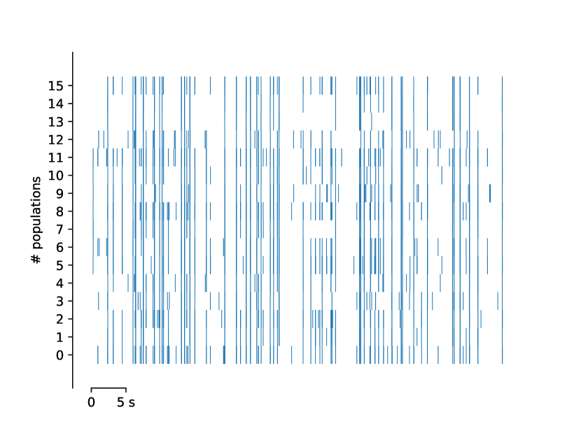
(a)

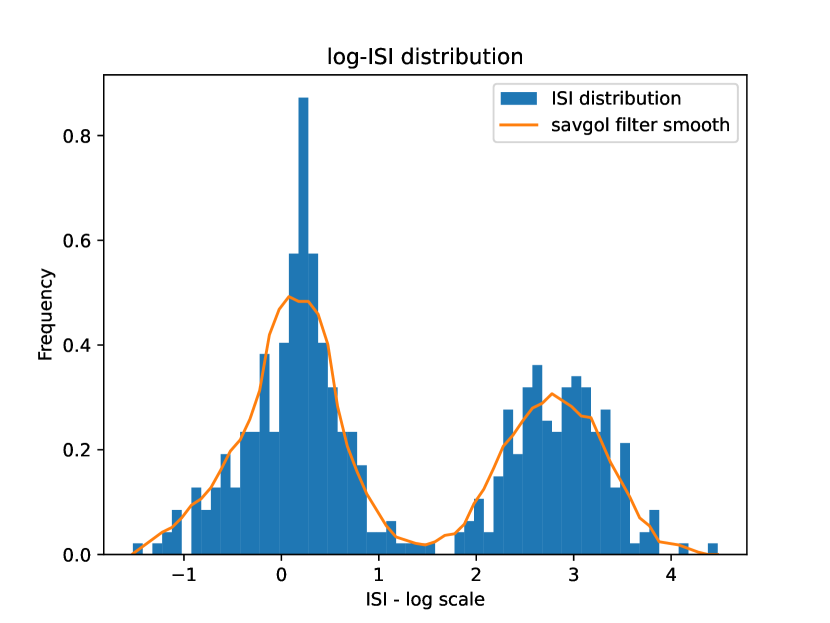
(b)

Figure 11: (a) Raster Plot of simulated electrophysiological activity of an in-silico network composed of 16 populations. (b) example of log-ISI distribution of population 0 of the same simulation depicted in the raster plot. The log-ISI histogram has been obtained as described in [31].

Moreover, as the RCN can be used to predict electrodes’ responses to a specific stimulus, we used the in-silico model to simulate such responses. For each stimulation protocol, a constant DC input lasting 2 ms was provided to all neurons of a specific population, for a total of 10 equally-spaced repetitions across 10 seconds length. One, or more stimulation protocols have been performed for each simulation by selecting a different targetpopulation, with 1 second of separation between each stimulation protocol. The starting and ending times of each repetition have been later used to compute the PSTH of the stimulated population. Different configurations have been tested with networks composed from 4 up to 60 populations. Each simulation was generated and simulated with different seed values for the random number generator of our simulation, leading each time to a different set of both intra- and inter-population connections. Moreover, each simulation lasted for five minutes, divided into two sections: a "background activity" section, lasting half of the recording, where only the noise and background components were active, and the "stimulation" section, where stimulation protocols could be performed in addition to the basal components. In particular, the background activity data was later used to train the RCN model and to calculate the Intrinsic Connectivity Matrix, while the stimulation data to perform response prediction tests.

Statistic

For Figure 3 (b), a Kruskal-Wallis H-test has been performed to calculate if the population median of all of the groups are equal considering each metric. Subsequently, a series of two-sided Mann-Whitney-Wilcoxon test with Bonferroni correction have been used to compare pairwise the algorithms performance.

Code details

All simulations were performed using the NEST simulator (version 3.5) [41] with custom code implemented in Python (version 3.8.17), with a kernel resolution of 0,01 ms. RCN model has been developed in Python implementing new classes on top of the ReservoirPy library (version 0.3.9) [42]. Common Python library, such as Numpy, Scipy, and Scikit-learn have been used throughout the custom code for analysis.

Code availability

The code for simulations, RCN model, and data analyses in this work will be available in public repository. Code can be shared upon request.

Data availability

The data of the simulations, recordings and data analyses reported in this study will be available in a public repository. Data can be shared upon request.

Supplementary Materials

I Experimental procedures

I.a Culture Preparation

In the preparation of primary neuron cultures, animals at 17/18 days of gestation were utilized, and all procedures conducted at the University of Trento in Italy strictly adhered to the approved ethical guidelines and regulations. To extract neurons from embryonic cortex tissue, we used the following protocol: initially, we decapitated the embryos and dissected their cortex under sterile conditions within a laminar flow cabinet, utilizing a standard dissection buffer enriched with glucose (HBSS). Afterward, we replaced the dissection buffer with 5ml of 0.25% trypsin-EDTA (Gibco) and allowed the tissues to incubate for 20 minutes in order to promote cell dissociation. Subsequently, to halt the action of trypsin, we introduced 5ml of DMEM medium supplemented with 10% FBS. We gently pipetted the solution and employed an appropriate strainer for neuron isolation. Following this, we subjected the separated cells to centrifugation at 1900 rpm for 5 minutes, effectively removing the superficial solution (DMEM,10% FBS, P/S). Finally, we added a seeding medium comprising DMEM, 10% FBS, and P/S until the cell concentration reached 1700 cells/$\mu$l. In our experimental procedure, we carefully dispensed 80$\mu$l of cell solution into each chip, employing a droplet technique and targeting the central region of the chips. These chips had been pre-coated with Poly-D-Lysine (PDL) and laminin. After a 2.5-hour incubation period, we proceeded to introduce the nourishing medium, consisting of Neurobasal supplemented with 1% B27, 1% Glutamax, and 1% P/S.

In order to ectopically express ChR2 in primary neuronal culture, we diluted 0.2$\mu$l of pAAV-hSyn-hChR2(H134R)-EYFP (#26973) in 100$\mu$l of standard feeding medium, which is composed of Penicillin-Streptomycin (10,000 U/mL) (1% v/v), GlutaMAX Supplement (1% v/v), B-27 supplement (50X) (2% v/v) and Neurobasal. All of these substances were purchased from Gibco. We then incubate the culture for 24 hours with the previously mentioned viral vector solution. Half of the medium was replaced with standard feeding medium following the incubation period. After six or seven days, the expression of EYFP can be used to track the expression of ChR2.

I.b MEA Recordings

The electrophysiological signals were recorded using MEA-2100mini system of Multichannel Systems GmbH (MCS). The microelectrode array chips used in our experiments were 60MEA-200/30iR-Ti-gr by MCS, which are chips with 60 titanium-nitride electrodes embedded in glass and surrounded by a glass ring. The electrodes are of 30$\mu$m diameter, where the horizontal and vertical spacing between each pair of electrodes is of 200$\mu$m. The MEA-2100mini system collects the signals through a headstage device. Then the signals undergo amplification and filtering. The system is then connected to a PC through an interface board. The recording is performed using MCS experimenter software, where the signals can be digitally filtered, inceptively-analyzed and tracked in real-time. We sampled the signals at 20KHz. The recorded files are then saved and exported for a secondary offline analysis

I.c Electrical Stimulation

The MEA-2100 mini system has also the feature of providing electrical stimulation to neuronal cultures. In our experiments, we applied bi-phasic square-shaped pulses with a peak-to-peak amplitude of 1.6V and a duration of 40 microseconds (20 microseconds for each phase) at a frequency of 0.5Hz for 300 repetitions.

I.d Optical Stimulation

In some experiments, we employed optical stimulation to activate ChR2-expressing neurons. This method enables a more precise and localized manipulation of neural activity, stimulating specific regions within the network, as opposed to the broader influence of electrical stimulation. As the light source we used a Digital Light Processor (DLP) system. The system is a DLP E4500, which includes 3 LEDs, optics, a WXGA DMD (Wide Extended Graphics Array Digital Micro-mirror Device) and a driver board. The light engine can produce approximately 150 lumen at 15W LED power consumption. The blue LED (488nm) which is used in this work has a power of 600mW. The light from the LEDs impinges on the DMD which has 1039680 mirrors arranged in 912 columns by 1140 rows with a diamond array configuration. Each of these mirrors has two main possible inclinations that reflect the light in a different direction. This system allows to get patterned illumination with pre-loaded and custom patterns that can be chosen through the DLP E4500 software. Moreover, these patters can be pulsed in time, with both an internal or external trigger, with a nominal precision down to $\mu$s. The system supports 1-, 2-, 3-, 4-, 5-, 6-, 7-, and 8-bit images with a 912 columns $\times$ 1140 rows resolution. These images are pixel accurate, meaning that each pixel corresponds to a micro-mirror on the DMD. The light coming from the DLP system is collimated and aligned to the optical path of the microscope from the rear port of the system. As can be seen in FIG. The light from the DLP is collected by a macro TAMRON 90mm AF2.5 objective and the light pattern is imaged on the sample plane, where the MEA chip is located, a by 10$\times$ objective, while passing through a dichroic mirror (Chroma T505lpxr-UF1) which acts like a high-pass filter, reflecting all the wavelengths smaller than 505nm.

The ChR2-infected culture could be in parallel imaged using a microscopy system, where the signal of the green fluorescent protein (GFP) expressed by the ChR2 infected cells, is transmitted through a dichroic filter and detected by a CMOS camera. The culture image allows to direct the desired light pattern from the DLP directly to the region of interest in the culture.

The light stimulation comprised 300 pulses of 20 milliseconds each, delivered as blue light at a frequency of 0.5 Hz (with 2-second intervals between pulses.)

II Data Pre-Processing

This sub-section details the electrophysiological data preprocessing method for the training datasets employed in the RC model. This process converts the raw electrical signals into data batches that capture episodes of notable culture activity. It’s worth noting that the intermediary algorithms within this procedure are flexible and can be tailored to specific requirements since they are not essential for the model’s functionality.

II.a Spike and Burst Detection

Following MEA recordings, the raw data was exported from MCS software and analyzed using a custom code written in Python. First the raw signals recorded on MEA were digitally filtered with a band-pass Butterworth filter with cutoff frequencies 0.3 and 3 KHz. Spikes were detected using the PTSD algorithm [33], setting the differential threshold (DF) to 8, refractory period (RP) to 1ms a

After detecting spikes, we proceeded to apply a burst detection algorithm inspired by the approach outlined in Ref. [31], but with some minor modification. By utilizing the spike trains, we derived the inter-spike intervals (ISI) for each channel within the recording. Subsequently, data from all channels was aggregated into a single ISI histogram, constructed with fixed bins of $\Delta\log_{10}\{ISI\}=0.1$ (in units of $\log_{10}$(s). The ISI threshold was then calculated by the following algorithm:

• Detect local maxima in the ISI histogram.

• Sort maxima by their significance, where significance is determined by $S_{peak}=p\cdot w$; $p$ is the peak prominence and $w$ is the peak full-width at half-prominence (FWHP).

• Choose the most significant peak within the bins between -3 and -2, corresponding to 1-10 $ms$, characterizing typical inter-burst intervals [31].

• Select the most significant peak within the bins spanning from -3 to -2, which corresponds to the range of 1 to 10 milliseconds. This peak characterizes the typical fast intra-burst intervals (for each channel).

• Choose the most significant peak within the bins greater than -2, corresponding to intervals longer than 10 milliseconds. This peak characterizes the typical inter-burst intervals (for each channel).

• calculate the ISI threshold by:

  $$\log_{10}(ISI_{th})=\frac{x_{l}+w_{l}/2+x_{r}-w_{r}/2}{2}$$ (31)

  where $x_{l},x_{r}$ are the bin value of the left and right peaks, respectively; $w_{l},w_{r}$ are the FWHP of the left and right peaks, respectively.

Following that, bursts were identified in each temporal sequence, provided that it contained a minimum of three spikes with inter-spike intervals $ISI^{(i,j)}\leq ISI_{th}$, where $i,j$ are the burst and channel indices, respectively. Consequently, bursts starting time $t_{B}^{i,j}$ were registered.

In the subsequent phase, we examined instances where bursting activity spread across the culture, indicating periods when bursts were detected on multiple channels within a specific time frame - also known as Network Bursts (NBs) [43]. NB was identified if burst occurred on at least two distinct channels $j$ and $k$ with respective starting times, $t_{B}^{j}$ and $t_{B}^{k}$, were separated by a time interval no greater than $\langle L_{B}\rangle/2$, where $\langle L_{B}\rangle$ is the average length of a burst. Consequently, NB starting times $t_{NB}^{j}$ were registered.

III Model Parametrization

We can categorize the model’s parameterization (Section 4) into three distinct types: fixed parameters- matrices $\mathcal{W}_{res}$, $\mathcal{W}_{in}$, and $\hat{\mathcal{S}}$; trainable parameters represented by $\mathcal{W}_{out}$; and hyperparameters $m$ and $\alpha$.

As discussed in Section 4, the fixed parameters consist of randomized matrices adhering to specific constraints. One of our key assessments of the model involved investigating the stability of the model’s predictions (connectivity or response) concerning the initialization of these fixed matrices. To achieve this, we conducted the training process a total of $N_{rep}$ times (typically between 5 and 10 repetitions) and examined the consistency of the model’s outcomes.

For instance, in the lasso regression (Eq. 3), the optimal $\mathcal{W}_{out}$ was determined for each set of $\mathcal{W}{res}$, $\mathcal{W}_{in}$, and $\hat{\mathcal{S}}$. We specifically evaluated the stability of connections within the intrinsic connectivity matrix (ICM), $\mathcal{T}_{0}$ (Eq. 6). This matrix results from the product of $\mathcal{W}{out}$ and $\hat{\mathcal{S}}$ with $\mathcal{W}{in}$. We assessed the consistency of connections in the ICM across different training sessions, quantifying it as the ICM confidence as follows:

$$\Gamma_{CM}=1-\frac{\max(\sigma_{\mathcal{T}_{0}})}{\max|\langle\mathcal{T}_{0}\rangle|}$$ (32)

Here, $\Gamma_{CM}$ represents the confidence value, $\sigma_{\mathcal{T}_{0}}$ stands for the standard deviation of the connection weights across the repetitions, and $\langle\mathcal{T}_{0}\rangle$ denotes the mean connection weights averaged over the repetitions. The assessment of response prediction stability, as outlined in Section 4.5.2, involved conducting the test with multiple initializations and calculating the mean response. The degree of stability is visualized by the error bars, which represent the standard deviation of the predicted response for each channel (Figs. 5(c) and 7(c) ,Section 4.5.2)

Regarding the hyperparameters $m$ and $\alpha$, we characterized their effect on model outcomes in all steps: Validation, Connectivity prediction and Response prediction. Fig. LABEL:fig:supp illustrates the characterization of some of the model’s metrics as a function of hyperparameters $m$ and $\alpha$.

IV External Test Parameters (Stimulation Intensity)

During the test phase where we examined how accurate the model can predict the network response to a given input (stimulus), we found that it is useful to tune the stimulation intensity as a fitting parameter in order to minimize the error between the ground truth response $\mathbf{U}$ and the prediction $\tilde{\mathbf{U}}$ in terms of $\bar{R}$ metric (Eq. (9)). Assuming that the stimulation is applied around node (electrode) $j$, we represent the input state (the stimulation) as:

$$\mathbf{u}_{in}=I\cdot\delta_{i,j}\;\;\;i=1,2,...,N_{ch}$$ (33)

where $I$ is the intensity and $\delta_{i,j}$ is the Kronecker delta.

V Performance Optimization

The model underwent training with a specific set of hyperparameters $(\alpha,m)$, as detailed in Section III. Each training set was iterated five times, employing different initializations for the fixed matrices of the model. During the testing phase, we assessed the trained model for each hyperparameter set using $\bar{R}$ and ROC AUC metrics (refer to Section 4.5.2). The primary optimization parameter was the stimulus intensity, outlined in Section IV. The optimal intensity was determined based on minimizing $\bar{R}$ for each combination of $\alpha$ and $m$. In instances where the $\bar{R}(I)$ characteristic exhibited a flat trend, the ROC AUC metric was employed as the arbitrator.

Subsequently, we generated maps of $\bar{R}(\alpha,m)$ and $AUC(\alpha,m)$ by averaging across various stimulation protocols. From these maps, we identified the optimal values for $m$ and $\alpha$. The optimal $m$ was regarded as a global parameter applicable to both stimulus testing and connectivity retrieval, as it is indicative of the network’s overall complexity and structure. In contrast, the optimal $\alpha$ was chosen independently for the stimulus test and connectivity, recognizing its dependence on specific operating regimes.

The optimization methodology employed in the model presented in this work hinges on test metrics rather than relying solely on training and validation phases. Anticipated is the need for fine-tuning the optimization process to align with the demands of real-time applications. Consequently, it is imperative to conduct additional studies to delve deeper into and refine this approach.

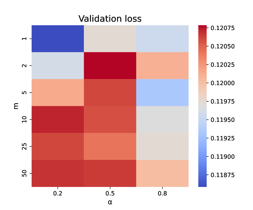
(a)

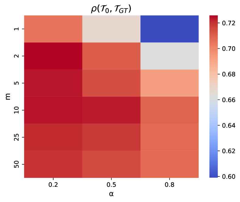
(b)

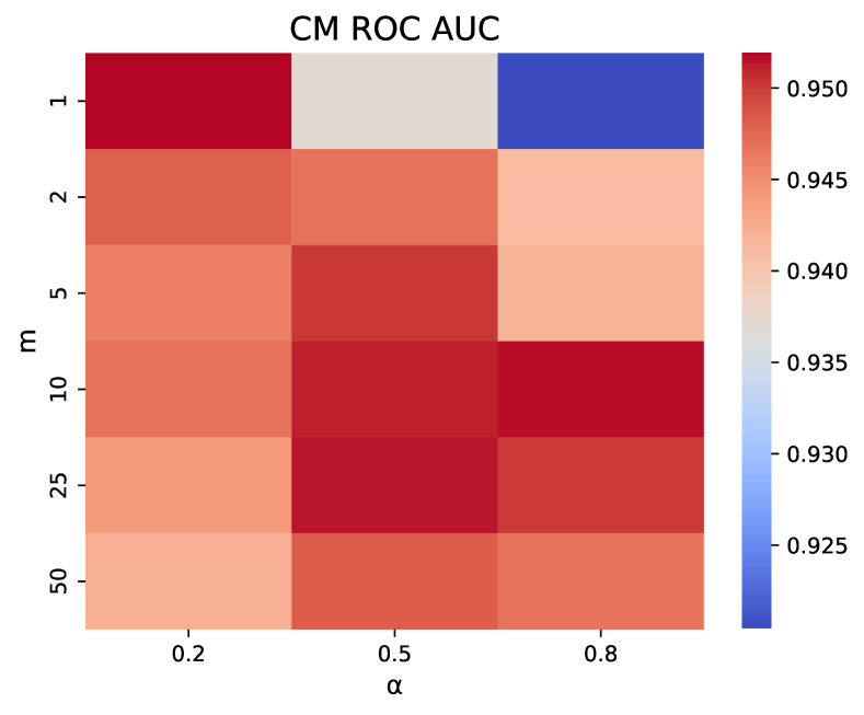
(c)

(d)

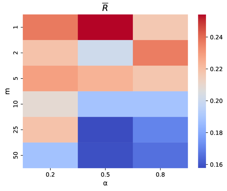
(e)

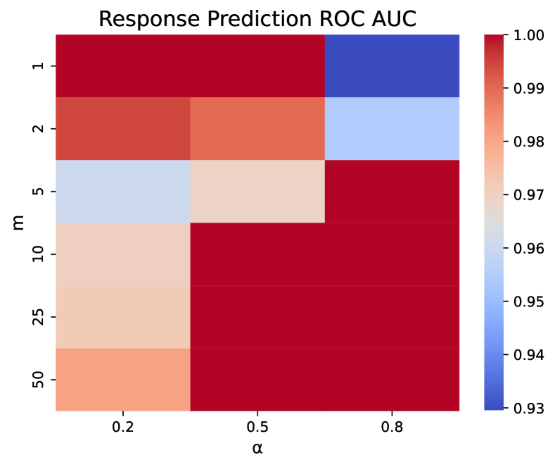
(f)

Figure 12: Parametrization of RC model estimators and metrics (dependence on hyperparameters $m$ and $\alpha$). All figures refer to results obtained from the same NEST simulation dataset presented in Figs 2 and 6. (a) validation loss (Eq. (19)). (b) Pearson correlation of the ICM with the ground truth connectivity matrix. (c) ROC AUC for the connectivity prediction. (d) Confidence measure of the ICM (Eq. (32)). (e) $\bar{R}$ metric of the response prediction. (f) ROC AUC metric for the response prediction.

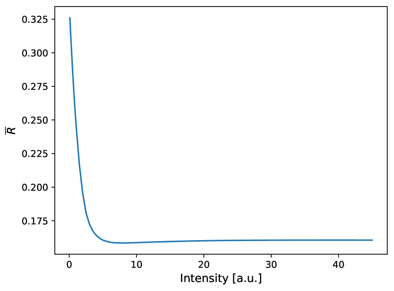
(a)

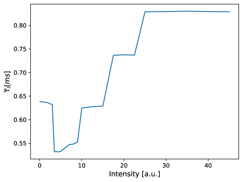
(b)

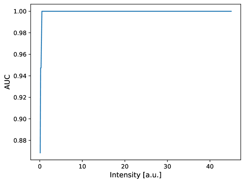
(c)

Figure 13: Response test metrics dependence on input intensity of the stimulus. The intensity was used as a tuning parameter to fit the model response to the experimental. (a) $\bar{R}$ (b) The overall time lag between the modeled response and the experimental, $\bar{\tau}_{l}$ (Eq. (30)). (c) ROC AUC.

VI More Supplementary Figures

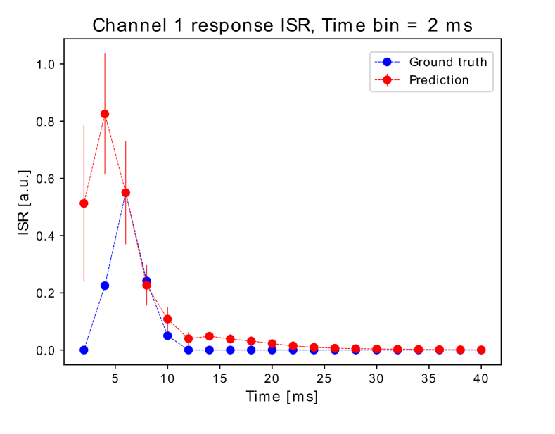
(a)

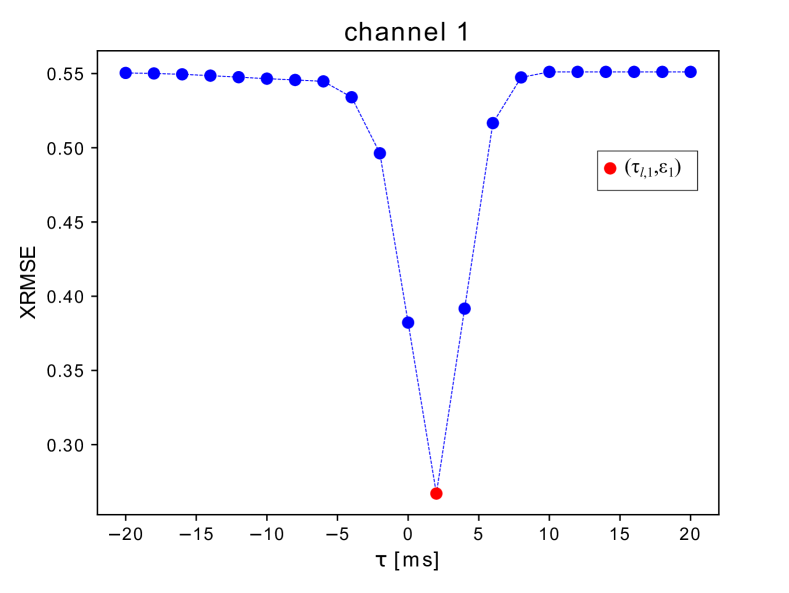
(b)

Figure 14: The principle of the XRMSE metric. (a) Ground truth and prediction data. (b) The outcome of XRMSE for the prediction of (a)- Eq. (26). The red point indicates the optimum point from which the channel error and the time lag ($\varepsilon_{i}$, $\tau_{l,i}$ Eq. (28)) are obtained. This procedure is done over all the channels of the network, followed by the total error, $\bar{R}$, and time lag, $\bar{\tau}_{l}$, estimation (Eqs. (29), (30)).

References

- [1] Rodolfo R Llinás. The intrinsic electrophysiological properties of mammalian neurons: insights into central nervous system function. Science, 242(4886):1654–1664, 1988.
- [2] Diego Contreras. Electrophysiological classes of neocortical neurons. Neural Networks, 17(5-6):633–646, 2004.
- [3] Alan L Hodgkin and Andrew F Huxley. A quantitative description of membrane current and its application to conduction and excitation in nerve. The Journal of physiology, 117(4):500, 1952.
- [4] Eve Marder and Adam L Taylor. Multiple models to capture the variability in biological neurons and networks. Nature neuroscience, 14(2):133–138, 2011.
- [5] Wulfram Gerstner and Werner M Kistler. Spiking neuron models: Single neurons, populations, plasticity. Cambridge university press, 2002.
- [6] Thomas Natschläger, Henry Markram, and Wolfgang Maass. Computer models and analysis tools for neural microcircuits. Neuroscience databases: a practical guide, pages 123–138, 2003.
- [7] Yuichiro Yada, Shusaku Yasuda, and Hirokazu Takahashi. Physical reservoir computing with force learning in a living neuronal culture. Applied Physics Letters, 119(17):173701, 2021.
- [8] Karl P Dockendorf, Il Park, Ping He, José C Príncipe, and Thomas B DeMarse. Liquid state machines and cultured cortical networks: The separation property. Biosystems, 95(2):90–97, 2009.
- [9] Mantas Lukoševičius and Herbert Jaeger. Reservoir computing approaches to recurrent neural network training. Computer science review, 3(3):127–149, 2009.
- [10] Donald H Perkel, George L Gerstein, and George P Moore. Neuronal spike trains and stochastic point processes: I. the single spike train. Biophysical journal, 7(4):391–418, 1967.
- [11] Emilio Salinas and Terrence J Sejnowski. Correlated neuronal activity and the flow of neural information. Nature reviews neuroscience, 2(8):539–550, 2001.
- [12] Thomas Schreiber. Measuring information transfer. Phys. Rev. Lett., 85:461–464, Jul 2000.
- [13] Sebastian Spreizer, Jessica Mitchell, Jakob Jordan, Willem Wybo, Anno Kurth, Stine Brekke Vennemo, Jari Pronold, Guido Trensch, Mohamed Ayssar Benelhedi, Dennis Terhorst, Jochen Martin Eppler, Håkon Mørk, Charl Linssen, Johanna Senk, Melissa Lober, Abigail Morrison, Steffen Graber, Susanne Kunkel, Robin Gutzen, and Hans Ekkehard Plesser. Nest 3.3, March 2022.
- [14] Robert Tibshirani. Regression shrinkage and selection via the lasso. Journal of the Royal Statistical Society: Series B (Methodological), 58(1):267–288, 1996.
- [15] Anthony Zador. Spikes: Exploring the neural code. Science, 277(5327):772–773, 1997.
- [16] Francesca Mastrogiuseppe and Srdjan Ostojic. Linking connectivity, dynamics, and computations in low-rank recurrent neural networks. Neuron, 99(3):609–623, 2018.
- [17] Valerio Mante, David Sussillo, Krishna V Shenoy, and William T Newsome. Context-dependent computation by recurrent dynamics in prefrontal cortex. nature, 503(7474):78–84, 2013.
- [18] Rodrigo Laje and Dean V Buonomano. Robust timing and motor patterns by taming chaos in recurrent neural networks. Nature neuroscience, 16(7):925–933, 2013.
- [19] Pierre Enel, Emmanuel Procyk, René Quilodran, and Peter Ford Dominey. Reservoir computing properties of neural dynamics in prefrontal cortex. PLoS computational biology, 12(6):e1004967, 2016.
- [20] Hongwei Cai, Zheng Ao, Chunhui Tian, Zhuhao Wu, Hongcheng Liu, Jason Tchieu, Mingxia Gu, Ken Mackie, and Feng Guo. Brain organoid reservoir computing for artificial intelligence. Nature Electronics, pages 1–8, 2023.
- [21] David Sussillo and Larry F Abbott. Generating coherent patterns of activity from chaotic neural networks. Neuron, 63(4):544–557, 2009.
- [22] Mark R Dranias, Han Ju, Ezhilarasan Rajaram, and Antonius MJ VanDongen. Short-term memory in networks of dissociated cortical neurons. Journal of Neuroscience, 33(5):1940–1953, 2013.
- [23] Han Ju, Mark R Dranias, Gokulakrishna Banumurthy, and Antonius MJ VanDongen. Spatiotemporal memory is an intrinsic property of networks of dissociated cortical neurons. Journal of Neuroscience, 35(9):4040–4051, 2015.
- [24] Tayfun Gürel, Stefan Rotter, and Ulrich Egert. Functional identification of biological neural networks using reservoir adaptation for point processes. Journal of computational neuroscience, 29:279–299, 2010.
- [25] Karl J Friston. Functional and effective connectivity: a review. Brain connectivity, 1(1):13–36, 2011.
- [26] Michela Chiappalone, Marco Bove, Alessandro Vato, Mariateresa Tedesco, and Sergio Martinoia. Dissociated cortical networks show spontaneously correlated activity patterns during in vitro development. Brain research, 1093(1):41–53, 2006.
- [27] Michela Chiappalone, Alessandro Vato, Luca Berdondini, Milena Koudelka-Hep, and Sergio Martinoia. Network dynamics and synchronous activity in cultured cortical neurons. International journal of neural systems, 17(02):87–103, 2007.
- [28] Guenter W Gross, E Rieske, GW Kreutzberg, and A Meyer. A new fixed-array multi-microelectrode system designed for long-term monitoring of extracellular single unit neuronal activity in vitro. Neuroscience letters, 6(2-3):101–105, 1977.
- [29] Michela Chiappalone, Valentina Pasquale, and Monica Frega. In vitro neuronal networks: From culturing methods to neuro-technological applications, volume 22. Springer, 2019.
- [30] Jan Müller, Marco Ballini, Paolo Livi, Yihui Chen, Milos Radivojevic, Amir Shadmani, Vijay Viswam, Ian L Jones, Michele Fiscella, Roland Diggelmann, et al. High-resolution cmos mea platform to study neurons at subcellular, cellular, and network levels. Lab on a Chip, 15(13):2767–2780, 2015.
- [31] Valentina Pasquale, Sergio Martinoia, and Michela Chiappalone. A self-adapting approach for the detection of bursts and network bursts in neuronal cultures. Journal of computational neuroscience, 29:213–229, 2010.
- [32] Douglas J Bakkum, Milos Radivojevic, Urs Frey, Felix Franke, Andreas Hierlemann, and Hirokazu Takahashi. Parameters for burst detection. Frontiers in computational neuroscience, 7:193, 2014.
- [33] Alessandro Maccione, Mauro Gandolfo, Paolo Massobrio, Antonio Novellino, Sergio Martinoia, and Michela Chiappalone. A novel algorithm for precise identification of spikes in extracellularly recorded neuronal signals. Journal of neuroscience methods, 177(1):241–249, 2009.
- [34] Vito Paolo Pastore, Aleksandar Godjoski, Sergio Martinoia, and Paolo Massobrio. S pi c o d yn: A toolbox for the analysis of neuronal network dynamics and connectivity from multi-site spike signal recordings. Neuroinformatics, 16:15–30, 2018.
- [35] Eugene M Izhikevich. Simple model of spiking neurons. IEEE Transactions on neural networks, 14(6):1569–1572, 2003.
- [36] Eugene M Izhikevich. Which model to use for cortical spiking neurons? IEEE transactions on neural networks, 15(5):1063–1070, 2004.
- [37] Priscila C Antonello, Thomas F Varley, John Beggs, Marimélia Porcionatto, Olaf Sporns, and Jean Faber. Self-organization of in vitro neuronal assemblies drives to complex network topology. Elife, 11:e74921, 2022.
- [38] Robert Gütig, Ranit Aharonov, Stefan Rotter, and Haim Sompolinsky. Learning input correlations through nonlinear temporally asymmetric hebbian plasticity. Journal of Neuroscience, 23(9):3697–3714, 2003.
- [39] Jonathan V Selinger, Nadezhda V Kulagina, Thomas J O’Shaughnessy, Wu Ma, and Joseph J Pancrazio. Methods for characterizing interspike intervals and identifying bursts in neuronal activity. Journal of neuroscience methods, 162(1-2):64–71, 2007.
- [40] Marie Engelene J Obien, Kosmas Deligkaris, Torsten Bullmann, Douglas J Bakkum, and Urs Frey. Revealing neuronal function through microelectrode array recordings. Frontiers in neuroscience, 8:423, 2015.
- [41] Marc-Oliver Gewaltig and Markus Diesmann. Nest (neural simulation tool). Scholarpedia, 2(4):1430, 2007.
- [42] Nathan Trouvain, Luca Pedrelli, Thanh Trung Dinh, and Xavier Hinaut. ReservoirPy: An efficient and user-friendly library to design echo state networks. In Artificial Neural Networks and Machine Learning – ICANN 2020, pages 494–505. Springer International Publishing, 2020.
- [43] J Van Pelt, MA Corner, PS Wolters, WLC Rutten, and GJA Ramakers. Longterm stability and developmental changes in spontaneous network burst firing patterns in dissociated rat cerebral cortex cell cultures on multielectrode arrays. Neuroscience letters, 361(1-3):86–89, 2004.