Near-Infrared Ca II Triplet As An Stellar Activity Indicator: Library and Comparative Study

Abstract

We have established and released a new stellar index library of the Ca II Triplet, which serves as an indicator for characterizing the chromospheric activity of stars. The library is based on data from the Large Sky Area Multi-Object Fiber Spectroscopic Telescope (LAMOST) Low-Resolution Spectroscopic Survey (LRS) Data Release 9 (DR9). To better reflect the chromospheric activity of stars, we have defined new indices $R$ and $R^{+}$. The library includes measurements of $R$ and $R^{+}$ for each Ca II infrared triplet (IRT) from 699,348 spectra of 562,863 F, G and K-type solar-like stars with Signal-to-Noise Ratio (SNR) higher than 100, as well as the stellar atmospheric parameters and basic information inherited from the LAMOST LRS Catalog. We compared the differences between the 3 individual index of the Ca II Triplet and also conducted a comparative analysis of $R^{+}_{\lambda 8542}$ to the Ca II H&K S and $R^{+}_{HK}$ index database. We find the fraction of low active stars decreases with $T_{eff}$ and the fraction of high active first decrease with decreasing temperature and turn to increase with decreasing temperature at 5800K. We also find a significant fraction of stars that show high activity index in both Ca II H&K and IRT are binaries with low activity, some of them could be discriminated in Ca II H&K $S$ index and $R^{+}_{\lambda 8542}$ space. This newly stellar library serves as a valuable resource for studying chromospheric activity in stars and can be used to improve our comprehension of stellar magnetic activity and other astrophysical phenomena.

1 Introduction

Stars with outer convective envelopes tend to exhibit magnetic activity. Star spots and faculae in the photosphere, plages in the chromosphere, X rays in the corona are all related to magnetic activity. Studies of stellar activity are essential for improving our understanding of stellar dynamo models and the related studies such as the stellar age and rotation or activity relation, stellar flare and stellar activity cycle. On the other hand, stellar activity is important for exoplanets studies, since magnetic activity especially flares will have an impact on planetary habitability (Shields et al., 2016; Howard et al., 2018; Lillo-Box et al., 2022). Also, jitters in both photometry and radial velocity measurement caused by stellar magnetic activity will hinder the detection of earth like exoplanet (Wright, 2005). Finding stars with low activity is crucial to those low mass exoplanets detecting.

The emission core of lines originated from the chromosphere can serve as indicators to quantify the activity. One well-known measure of activity is the Ca II H&K $S_{MWO}$ index, proposed by the Mount-Wilson Observatory (Wilson, 1968). However, the photosphere also contributes to the Ca II H&K lines flux, and the contribution varies with effective temperatures, leading to potential misestimation of the stellar activity. To overcome this issue, Linsky et al. (1979) proposed the $R^{\prime}_{HK}$ index, which subtracts the empiprical photospheric flux from the flux. Building on the $R^{\prime}_{HK}$ index, Mittag et al. (2013, 2019) proposed the $R^{+}_{HK}$ index, which subtracts the basal flux in addition to the photospheric flux. $H_{\alpha}$ line can also serve as an indicator of activity, and is more suitable for late-type stars than Ca II H&K (Cincunegui et al., 2007). They defined the $S^{+}$ index for $H_{\alpha}$, which correlates well with the $S_{MWO}$ index.

The Ca II IRT lines represent another set of indices of activity:

$$8498.0\mathring{A}\ 4\ ^{2}P_{\frac{3}{2}}-3\ ^{2}D_{\frac{3}{2}},$$

$$8542.1\mathring{A}\ 4\ ^{2}P_{\frac{3}{2}}-3\ ^{2}D_{\frac{5}{2}},$$

$$8662.1\mathring{A}\ 4\ ^{2}P_{\frac{1}{2}}-3\ ^{2}D_{\frac{3}{2}},$$

absorptions due to the Ca II IRT lines are clearly visible in the atmosphere of cool stars (see Tennyson, 2019, chap. 6). The Ca II IRT emission lines core are formed in the lower chromosphere through subordinate transitions between the excited levels of Ca II $4\ ^{2}P_{\frac{3}{2},\frac{1}{2}}$ and meta-stable $3\ ^{2}D_{\frac{3}{2},\frac{5}{2}}$. These lines are mostly collision controlled (de Grijs & Kamath, 2021), and are highly sensitive to the ambient temperature (Cauzzi et al., 2008). They are indicator of stellar chromospheric activity, as demonstrated by Linsky et al. (1979). Linsky et al. (1979) proposed using Ca II $\lambda 8542$ as an activity indicator, while Andretta et al. (2005) defined the $R_{IRT}$ index based on the central depression in the Ca II IRT lines, taking into account rotational broadening. Notsu et al. (2015) used $r_{0}(IRT)$, which is the residual flux normalized by the continuum at the line cores of IRT lines, and $H_{\alpha}$ to study superflare and suggested that the brightness variation of superflare stars can be explained by the rotation with large starspots. Žerjal et al. (2013) use observed spectra of non-active stars as template, and measure the template subtracted equivalent width(EW) of the Ca II IRT lines to represent the stellar activity.

It is important to built large databases to statistically understanding the physical mechanisms of stellar magnetic activity. As a series of work, we have already built large sample databases of stellar activity of solar like stars using Ca II H&K (Zhang et al., 2022) and $\rm H_{\alpha}$ (He et al., 2023) index based on LAMOST spectra. In the current work, we will build a stellar activity database of F, G, K stars based on the measurement of Ca II IRT lines.

LAMOST, the Large Sky Area Multi-Object Fiber Spectroscopic Telescope located in Xinglong, China, offers low-resolution spectra with a resolving power of $\lambda/\Delta\lambda=1800$ covering the wavelength range of 3700-9100 $\mathring{A}$ (Zhao et al., 2012). Additionally, it provides Mid-Resolution Spectra (MRS) with $R\sim 7500$ in 4950-5350 $\mathring{A}$, 6300-6800$\mathring{A}$ band. The observed data was first reduced by LAMOST 2D pipeline (Bai et al., 2017, 2021), then LAMOST stellar parameter pipeline (Wu et al., 2011). The released data including extracted spectra files as well as the stellar parameters are available at the LAMOST website, http://www.lamost.org.

There have been several studies of stellar activity based in LAMOST data. For example, Zhang et al. (2020) employed the $R^{+}_{HK}$ index to investigate the relationship between stellar activity, period, and the amplitude of brightness variation; He et al. (2023) measured the $R_{H_{\alpha}}$ index using LAMOST MRS; Zhang et al. (2022) established Ca II H&K $S$ index database base on LAMOST LRS; Karoff et al. (2016) explored superflares using the $S$ index and found that superflare stars are characterized by enhanced activity; Zhang et al. (2019) proposed that stellar chromospheric activity indices can be used to roughly estimate stellar ages for dwarfs. The above studies are based on the measurement of Ca II H&K or $H_{\alpha}$, the capability of Ca II IRT lines has not been fully explored yet.

In this study, we concentrate on Ca II IRT lines of solar-like stars, all the spectra utilized in our research come from the LAMOST LRS DR9 database. Due to the low spectral resolution, the line core emission is not sensitive to equivalent width (EW) and may be compromised by deviations in rotation velocity estimations. Instead, we introduce a new $R$ index that specifically considers the flux near the center of spectral lines. To remove the photospheric flux components, we employed the BT-Settl stellar spectral models ((Allard et al., 1997, 2011, 2013) and calculate the template subtracted index, $R^{+}$, to represent pure activity levels. Additionally, we compare our results with the existing database of Ca II H&K lines and discuss the nature of stars in the Ca II H&K and IRT activity index distribution.

This paper is organized in five sections. Section 2 introduces the data selection criteria, while Section 3 defines the indices $R$ and $R^{+}$ and provides a detailed description of the data processing steps. Section 4 shows the detail of our database. In Section 5 we compared the strengths of the three lines, discusses the relationship and differences between the indices measured from Ca II H&K. Section 6 is the summary.

2 Data Preparation

Our analysis focuses on F, G and K-type solar-like stars, with all stellar parameters sourced from the catalog: LAMOST LRS Stellar Parameter of A, F, G, and K Stars (AFGK Catalog) (http://www.lamost.org/dr9/). To be comparable with the previous Ca II H&K index work of Zhang et al. (2022), the following parameter restrictions are adopted:

1. $100\leq SNR_{i},\ SNR_{z}$. This is to ensure the high quality of the Ca II IRT lines located between i & z band.

2. $4800K\leq T_{eff}\leq 6800K$, This criterion is same as Zhang et al. (2022), the temperature range of solar-like stars covers most F, G, K samples in the AFGK Catalog.

3. For surface gravity, the empirical formulas of Zhang et al. (2022) is adopted to select main sequence stars:

   $$5.98-0.00035T_{eff}\leq\text{log}\ g\leq 5.0$$

After rejecting spectra with issues such as fiber failure at the IRT bandpass, heavy skylight pollution, and wavelength calibration failure, we selected a total of 699,348 spectra from the LAMOST database. As there are multiple visits for the same star, these spectra are from 562,863 stars. The number of spectra cross-correlated with the previous work of Ca II H&K $S$ and $R^{+}_{HK}$ index databases is listed in Table 1.

Table 1: Ca II index Database Using LAMOST Data

Database	Spectra Number	Common Spectra
Ca II IRT $R$, $R^{+}$	699348	-
Ca II H&K $S$	1330654	574780
Ca II H&K $R^{+}_{HK}$	59816	14028

3 Method

3.1 Index definitions

We defined $R$, $R^{+}$ index for each line of Ca II IRT as following equations:

$$R=\frac{1}{\lambda_{2}-\lambda_{1}}\int^{\lambda_{2}}_{\lambda_{1}}\frac{F_{o}(\lambda)}{C_{o}(\lambda)}\ d\lambda,$$ (1)

$$R^{+}=\frac{1}{\lambda_{2}-\lambda_{1}}\int^{\lambda_{2}}_{\lambda_{1}}\frac{F_{o}(\lambda)}{C_{o}(\lambda)}-\frac{F_{m}(\lambda)}{C_{m}(\lambda)}\ d\lambda,$$ (2)

where $F(\lambda)$ is the spectrum, $C(\lambda)$ is the linear function fitting the local continuum at IRT bandpass, and subscript o and m stand for observation and model respectively. $F(\lambda)/C(\lambda)$ is the normalized spectrum. $\lambda_{1}$, $\lambda_{2}$ are the starting and ending wavelength of the sampling range, which is 1$\mathring{A}$ around the central wavelength of each Ca II IRT lines. The corresponding central wavelengths and the sampling ranges are listed in Table LABEL:tab2. As the LAMOST spectral data points are in approximately 2$\mathring{A}$ interval, a cubic spline function is applied to interpolate the spectrum to 0.001$\mathring{A}$ interval.

Table 2: Sampling Range for Ca II IRT Index

Lines	Center$(\mathring{A})$	Bandpass$(\mathring{A})$
Ca II $\lambda 8498$	8500.35	8549.85-8500.85
Ca II $\lambda 8542$	8544.44	8543.94-8544.94
Ca II $\lambda 8662$	8664.52	8664.02-8665.02

LAMOST DR9 provides normalized spectra for most spectra, these are typically generated for the entire spectrum. To achieve better performance, we re-normalized the spectra within the IRT bandpass with a normalization method that utilizes the LinearLSQFitter provide by Astropy module, which is a linear least square fitting method (Robitaille et al., 2013; Price-Whelan et al., 2018, 2022). Two examples are illustrated in Figure 1 to show the difference between global and local normalization. Both methods perform similarly for the absorption line spectra, but in the case of emission lines, our method clearly outperforms the LAMOST approach.

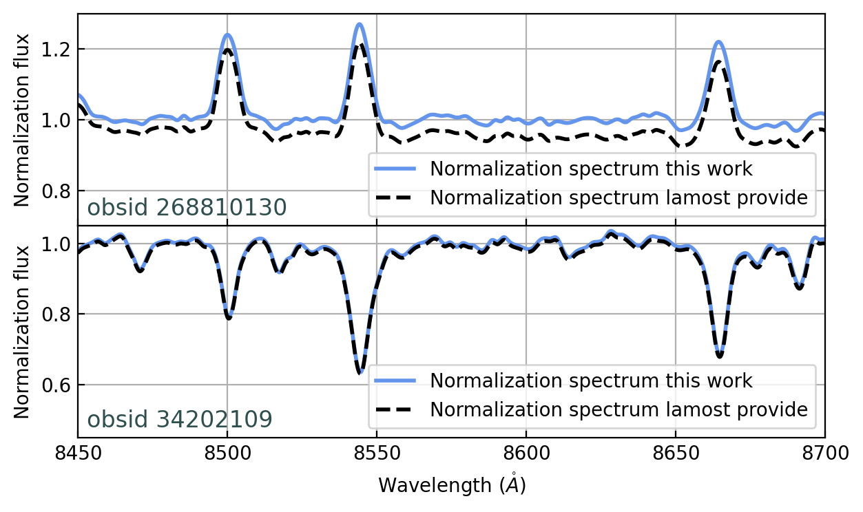
Figure 1: Comparison of different normalization in the Ca II IRT region. the upper panel is the emission lines spectrum and the lower is the absorption lines spectrum. The blue curve is the local normalized spectra by this work and the black curve is the global normalized spectra provided by LAMOST DR9.

3.2 Templates

For late type stars. the dissipation of acoustic energy (Schrijver et al., 1989) and turbulent dynamo activity from non-rotating plasma (Bercik et al., 2005) in the upper photosphere contribute to the line core of Ca II H&K and Ca II IRT lines, thus it is better to subtract this ”basal” flux from the spectrum to derive the true chromosphere activity. Andretta et al. (2005) studied the non-local thermodynamic equilibrium (NLTE) effect contribution of Ca II IRT lines, and found that the Central-Depression(CD) index can be affected by NLTE by more than 20%. As our $R^{+}$ and $R$ indices are defined on narrow band of 1Å, similar to CD index, NLTE should be consider in $R^{+}$ index to remove the basal flux. The LTE BT-Settl spectral model and NLTE model for Ca II lines (Allard et al., 2013) based on Phoenix (Husser et al., 2013) code were applied to subtract the basal flux in Ca II IRT region.

The grids of BT-Settl templates are listed in Table 3. These templates were interpolated with intervals of $\Delta T_{eff}=10K$, $\Delta\text{log}\ g=0.01$ and $\Delta[Fe/H]=0.01$ to ensure a precise match with our observational spectra. The templates are degraded to $R\approx 1800$ and subtracted from the observed spectra, as equation 2.

Table 3: Parameter Space of The Grid

Parameter	Range	Grid Size
$T_{eff}$(K)	4800-6800	100
$\text{log}\ g$	3.5-5.0	0.5
$[Fe/H]$	[-1.0,-0.5,0,0.3,0.5]	-
$[\alpha/Fe]$	0.0-0.4	0.2

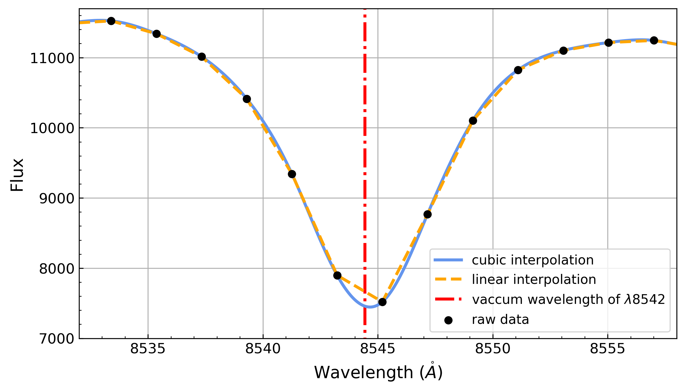
Figure 2: Difference of two interpolation method. Black dots are observed spectrum; Blue curve is the cubic spline interpolation of the spectrum; Orange dash curve is the linear interpolation; Red dot-dash line shows the vaccum wavelength of $\lambda 8542$.

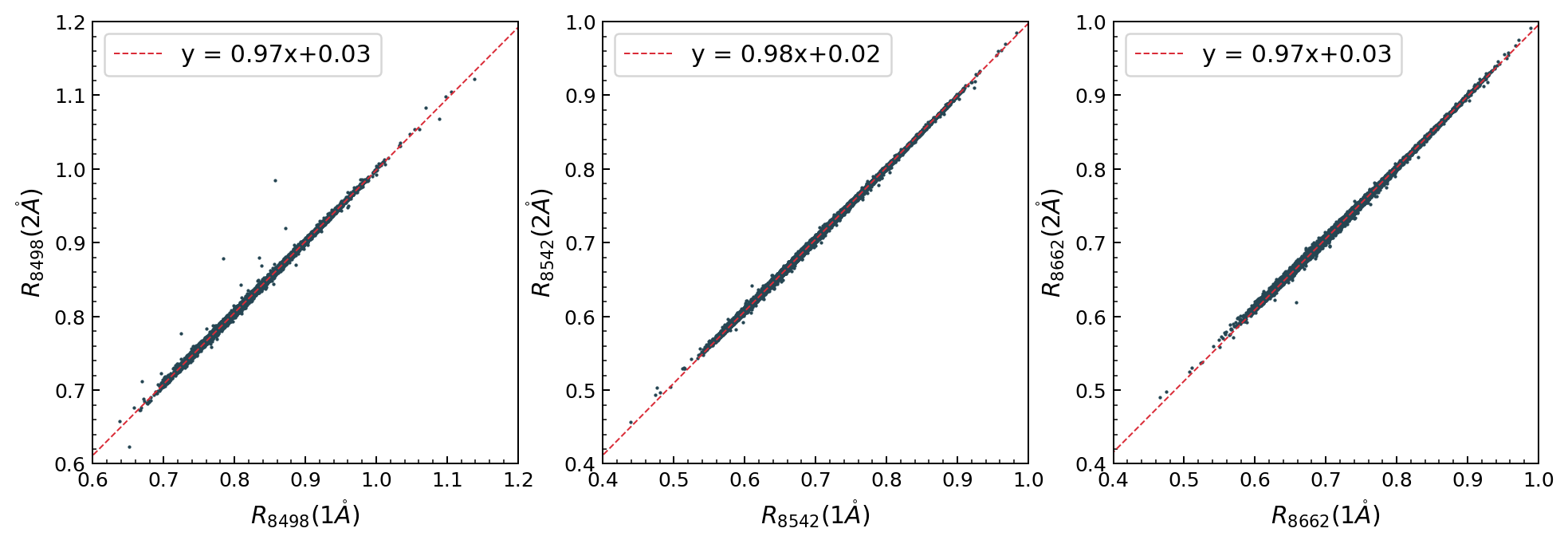
Figure 3: Comparison of $R$ index derived from 1 $\mathring{A}$ and 2 $\mathring{A}$ width respectively for each IRT line. Red dash line is obtained by least squares fitting of the data.

3.3 Uncertainties Estimation

Similar to the LAMOST Ca II H&K index error budget analysis in Zhang et al. (2022) , for Ca II IRT $R$ index, we consider three factors of uncertainty as follows:

1. Uncertainty of spectral flux. LAMOST release the targets spectrum as well as the corresponding spectra of inverse variance($1/\delta^{2}$), which could be used to estimate the flux uncertainty:

   $$\delta R_{flux}=\sqrt{\frac{1}{\lambda_{2}-\lambda_{1}}{\int^{\lambda_{2}}_{\lambda_{1}}(\frac{\delta(\lambda)}{C(\lambda)})^{2}}\ d\lambda},$$ (3)

   where $C(\lambda)$ is the continuum, same as defined in equation 1.

2. Uncertainty of interpolation. As the wavelength interval of LAMOST spectra is 2Å, the spectrum are interpolated. Different interpolation method lead to the uncertainty of $R$ index, as illustrated in Figure 2. The uncertainty of interpolation is derived as:

   $$\delta R_{interpolation}=|R_{cubic}-R_{linear}|,$$ (4)

   to ensure that our choice of 1 Å window doesn’t impact our conclusions, we compared the $R$ indices of each Ca II IRT line measured in 1 $\mathring{A}$ window with those of the 2 $\mathring{A}$ window. For majority of targets, the difference is negligible, as shown in Figure 3.

3. Uncertainty of red shift(or radial velocity). by applying $z+z_{err}$, $z$, $z-z_{err}$ offered by LAMOST DR9, we can obtain the $R_{+}$, $R$, $R_{-}$ respectively for each line, so $\delta R_{z}$ is shown as following:

   $$\delta R_{z}=\frac{|R-R_{+}|+|R-R_{-}|}{2}.$$ (5)

Combining function 3,4 and 5, the total error $\delta R$ is give by,

$$\delta R=\sqrt{\delta R_{flux}^{2}+\delta R_{interpolation}^{2}+\delta R_{z}^{2}}.$$ (6)

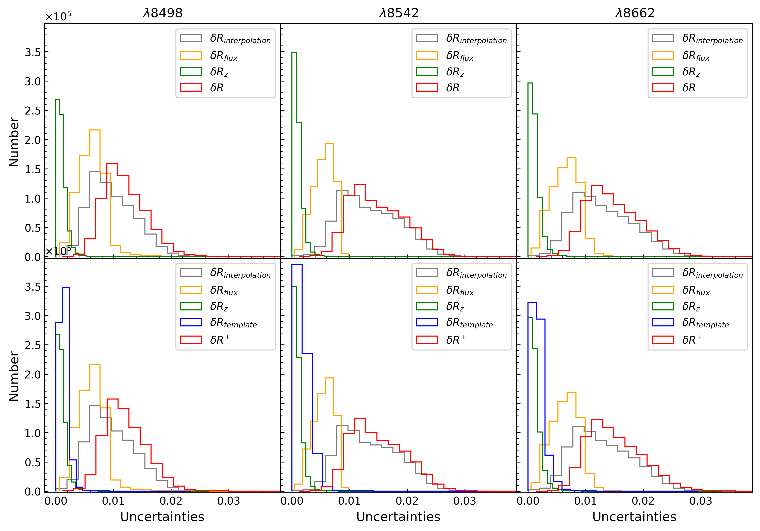
Figure 4: Distribution of uncertainties for the spectral lines $\lambda 8498$, $\lambda 8542$, and $\lambda 8662$ in three columns from left to right. Each column includes two panels, with the top one showing the distribution of uncertainty for $R$ and its individual component, and the bottom one displaying the distribution of uncertainty for $R^{+}$, both represented by the red histogram.

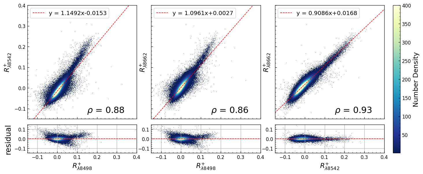
Figure 5: Linear regression was performed for each pair of $R^{+}$ values in IRT, with the corresponding residuals between the data and the fitted line shown in the lower panels. The left column displays $R^{+}_{\lambda 8498}$ - $R^{+}_{\lambda 8542}$, the middle column shows $R^{+}_{\lambda 8498}$ - $R^{+}_{\lambda 8662}$, and the right column depicts $R^{+}_{\lambda 8542}$ - $R^{+}_{\lambda 8662}$. The red dashed lines represent the regression equation obtained from fitting the data, while $\rho$ corresponds to the Pearson correlation coefficient.

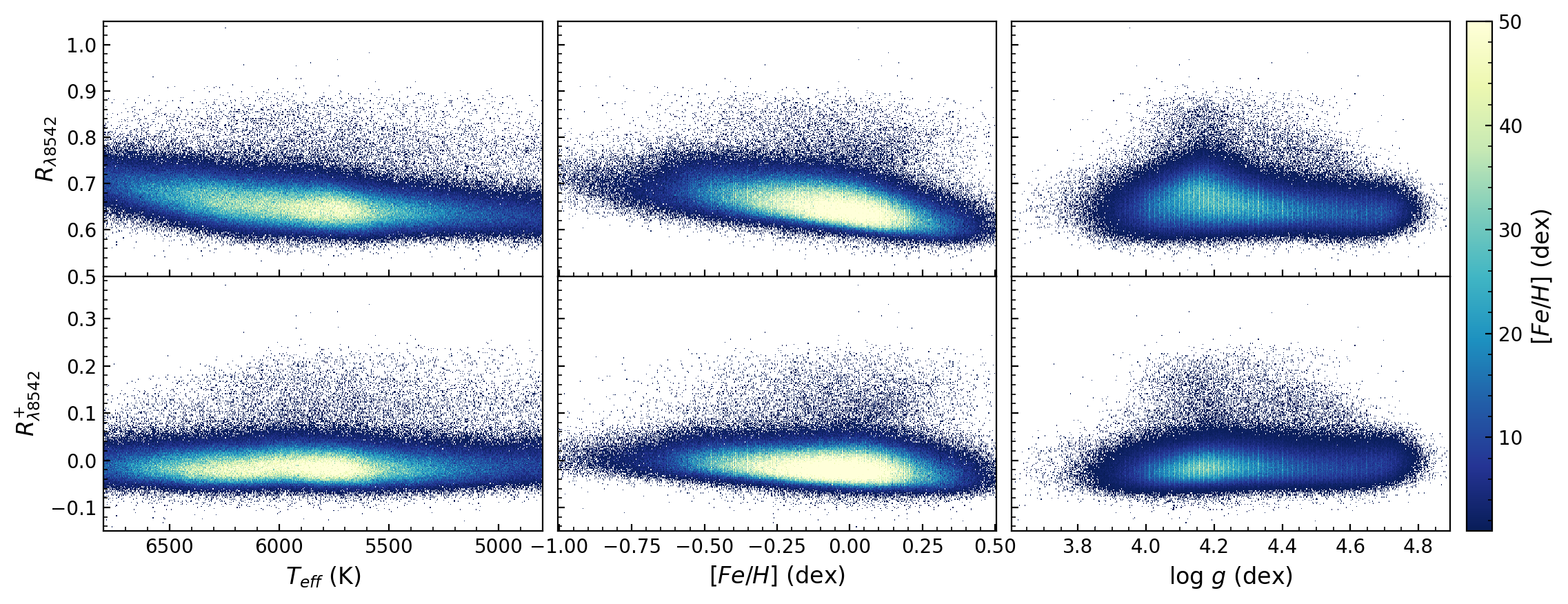
Figure 6: The distribution of $R_{\lambda 8542}$ and $R^{+}_{\lambda 8542}$ with stellar parameters. From top to bottom are $T_{eff}$, $[Fe/H]$ and $\text{log}\ g$, respectively. The upper section in each panel is $R$ index and the lower is for $R^{+}$, as indicated in the plot.

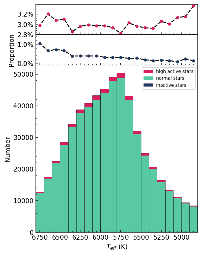
Figure 7: Top and mid panels shows the proportion of high active stars and inactive stars, respectively. The bottom panel shows the number count of different category in different temperature bins, as indicated by different color.

For $R^{+}$ index, the additional uncertainty comes from the templates uncertainty. According to the stellar parameter error offered by LAMOST DR9, we calculate a serious of $R$ index for each templates around the best template, [$T_{eff}\pm\Delta T$, $\text{log}\ g\pm\Delta\text{log}\ g$, $[Fe/H]\pm\Delta[Fe/H]$]. The maximum and minimum of the template index $R_{T}$ are denoted as $R_{T}^{max}$ and $R_{T}^{min}$ respectively. Then uncertainty of template index $R_{T}$ is

$$\delta R_{T}=max(|R_{T}-R_{T}^{max}|,\ |R_{T}-R_{T}^{min}|),$$ (7)

and the uncertainty of $R^{+}$ is

$$\delta R^{+}=\sqrt{\delta R^{2}+\delta R_{T}^{2}}.$$ (8)

Figure 4 shows the contribution of different components to $\delta R$ and $\delta R^{+}$, we can see that the uncertainty of $R^{+}$ is mainly dominated by the uncertainty of interpolation and flux error.

4 Stellar Activity Database

We calulated the $R$ and $R^{+}$ index and the corresponding error for 699,348 F, G and K-type spectra selected from LAMOST DR9 database. The results are written in a CSV form table and uploaded to the website https://nadc.china-vo.org/res/r101246/. The description of columns of the database could be found in Table LABEL:tab4. Our R and $R^{+}$ index database could be used as indicator for stellar activity studies. Theoretically, the $R^{+}$ index is close to zero for inactive stars, but there are a large fraction of stars with the $R^{+}$ index below zero (see Figure 6). The similar negative value are also found in GAIA (Lanzafame et al., 2023) and RAVE (Žerjal et al., 2013) Ca II IRT index measurement. We believe that the following reasons have led to this:

1. The parameters of LAMOST may not have been measured accurately.

2. Low or moderate chromospheric activity could produce some extra absorption (Mullan, 1979; Lanzafame et al., 2023).

Table 4: Columns of catalog

Column	Unit	Description
obsid		LAMOST observation identifier
gaia_source_id		Source identifier in Gaia DR3
gaia_g_mean_mag		G mag provided by Gaia DR3
snri		SNR at i band
snrz		SNR at z band
ra_obs	degree	RA of fiber point
dec_obs	degree	DEC of fiber point
teff	K	$T_{eff}$, Effective temperature
teff_err	K	Uncertainty of $T_{eff}$
logg	dex	$\text{log}\ g$, Surface gravity
logg_err	dex	Uncertainty of $\text{log}\ g$
feh	dex	$[Fe/H]$, Metallicity
feh_err	dex	Uncertainty of $[Fe/H]$
rv	km/s	$V_{r}$, Radial velocity
rv_err	km/s	Uncertainty of $V_{r}$
R_8498		$R_{\lambda 8498}$
R_8498_err		uncertainty of $R_{\lambda 8498}$
R_8542		$R_{\lambda 8542}$
R_8542_err		uncertainty of $R_{\lambda 8542}$
R_8662		$R_{\lambda 8662}$
R_8662_err		uncertainty of $R_{\lambda 8662}$
R_plus_8498		$R^{+}_{\lambda 8498}$
R_plus_8498_err		uncertainty of $R^{+}_{\lambda 8498}$
R_plus_8542		$R^{+}_{\lambda 8542}$
R_plus_8542_err		uncertainty of $R^{+}_{\lambda 8542}$
R_plus_8662		$R^{+}_{\lambda 8662}$
R_plus_8662_err		uncertainty of $R^{+}_{\lambda 8662}$

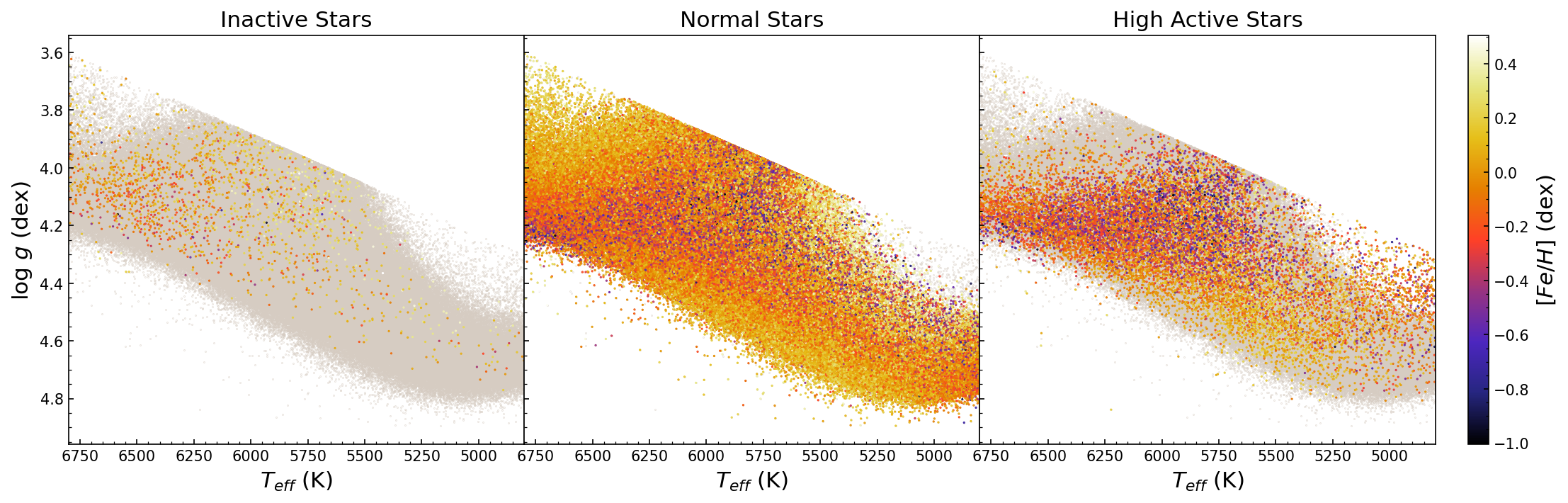
Figure 8: Distribution of inactive, normal and high active stars in the $T_{eff}$ and $Logg$ space, different color represent different [Fe/H], as indicated by the color bar.

5 Discussion

5.1 Relationship between IRT indices and stellar parameters

In Figure 5, we plot the Ca II IRT $R^{+}$ index against each other. There is a clear linear correlation in each plot. We calculated the Pearson correlation coefficient and marked at the lower part of each panel. For each pair, the ridge of the density distribution is fitted with a linear function using the Bayesian Ridge Regression algorithm from the sklearn module (Pedregosa et al., 2011). The functions are shown on the top of each panel of Figure 5. From the figure, we can see that $R^{+}_{\lambda 8542}-R^{+}_{\lambda 8662}$ exhibit the strongest linear relationship, with a higher Pearson coefficient than other pairs. The $\lambda 8542$ line is the most opaque member of the Ca II IRT lines and usually considered as a better diagnostic for the chromospheric activities (Linsky et al., 1979). According to the linear function slopes, the strength of $R^{+}_{\lambda 8542}$ is stronger than the other two lines, our results confirms the conclusion of Linsky et al. (1979) and are also consistent with the results of Žerjal et al. (2013) and Martin et al. (2017). Henceforth, we limit our discussion to $\lambda 8542$, although all the other line index are available in our database for possible use.

The distributions of $R^{+}_{\lambda 8542}$ and $R_{\lambda 8542}$ with stellar parameters are presented in Figure 6. Stars with low activity is also important for low mass exoplanets studies since life may more possibly exist in a planet hosted by low active star and exoplanet may be more easily discovered around low active stars than the active because both the observed lightcurve and radial velocity curve will be more stable due to less spots on the star (e.g. Korhonen et al., 2015; Hojjatpanah et al., 2020). To take a peek at the distribution of the chromospheric active and inactive stars, the star are divided into 20 temperature bins, and the number count in each bins are plotted in the bottom panel of Figure 7. The mean and variance of $R^{+}_{\lambda 8542}$ are calculated for each bin. Stars with $R^{+}$ index higher than 2$\sigma$ are defined as active stars and lower than 2$\sigma$ are inactive stars. The fractions of active and inactive stars are plotted in the upper 2 panels of Figure 7. The fraction of inactive stars decrease with temperature. While the fraction of active stars increase with the decreasing temperature below 5800K, and increase with temperature above 5800K. As there are a large fraction of high $R$ index stars are actually binaries (see Section 5.2 below), the increasing of active star fraction with temperature may reflect the increasing binary fraction with mass rather than the increasing activity. Further work is needed to make it clear. The distributions of active, inactive and normal stars in the stellar parameter space are shown in Figure 8. The inactive stars show high metallicity in Figure 8 , indicating that they are thin disk population, similarly, the low metallicity population in the active stars plot may possibly comes from the local thick disk population. As some stars were observed several times by LAMOST, for Figure 6, 7 and 8, only one spectrum were kept for stars with multiple visits to ensure the fraction is not biased by repeat count. As the stellar activity is a complicated function of mass, age, metallicity and rotation, which is beyond the scope of the current paper, we will leave the detail analysis for the future work.

5.2 Comparing with S index

Comparing our database with Ca II $H\&K$ $S$ index of Zhang et al. (2022), there are 0.58 million spectra in common(Table 1). The $S$ index VS $R^{+}_{\lambda 8542}$ and $S$ VS $R_{\lambda 8542}$ are plotted in Figure 9. Both plots show linear relation between $S$ index and $\lambda 8542$ indices, with $R^{+}$ is less scattered than $R$ index as the basal photospheric contribution was removed.

Visually inspecting Figure 9, the high activity index star seems to be divided into 3 branches. We label those 3 branches in Figure 10 and plot their distributions in stellar parameter space in the lower panels of Figure 10 respectively. For Branch 1, we did not find any specific tendencies in the distribution of $T_{eff}$, $[Fe/H]$, but they almost located at $\text{log}\ g<4.5$. Branch 2 has lower $R^{+}$ index than Branch 1 and extend to very high $S$ index end. They distributed at temperatures below 5750K and exhibits high metallicity. Branch 3 has high $S$ index but low $R^{+}_{\lambda 8542}$ index. The sample size of Branch 3 is small, but they has a broad temperature range. They shows high metallicity in the low-temperature end and low metallicity in the high temperature end.

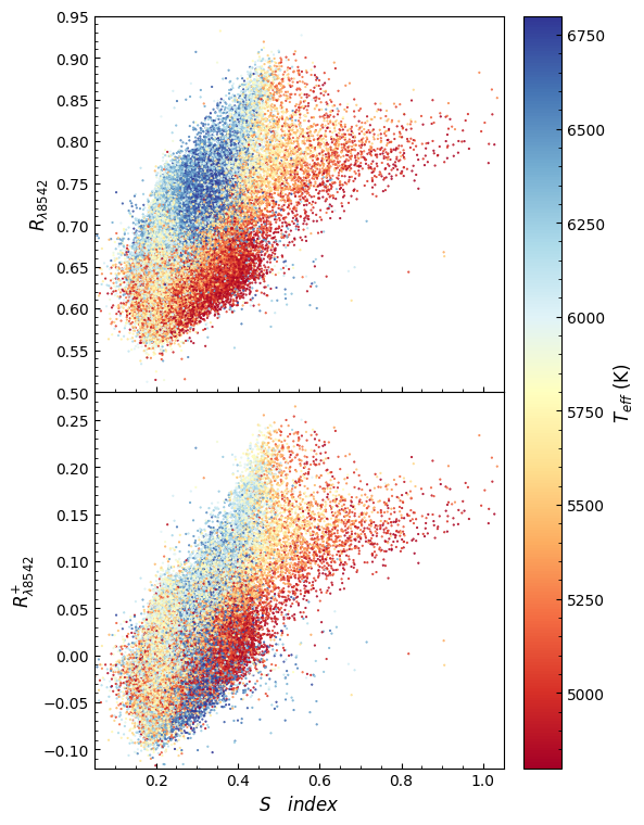
Figure 9: Top panel is the relationship of $S$ index and $R_{\lambda 8542}$, bottom panel is the relationship of $S$ index and $R^{+}_{\lambda 8542}$. Colors of each point show the temperature.

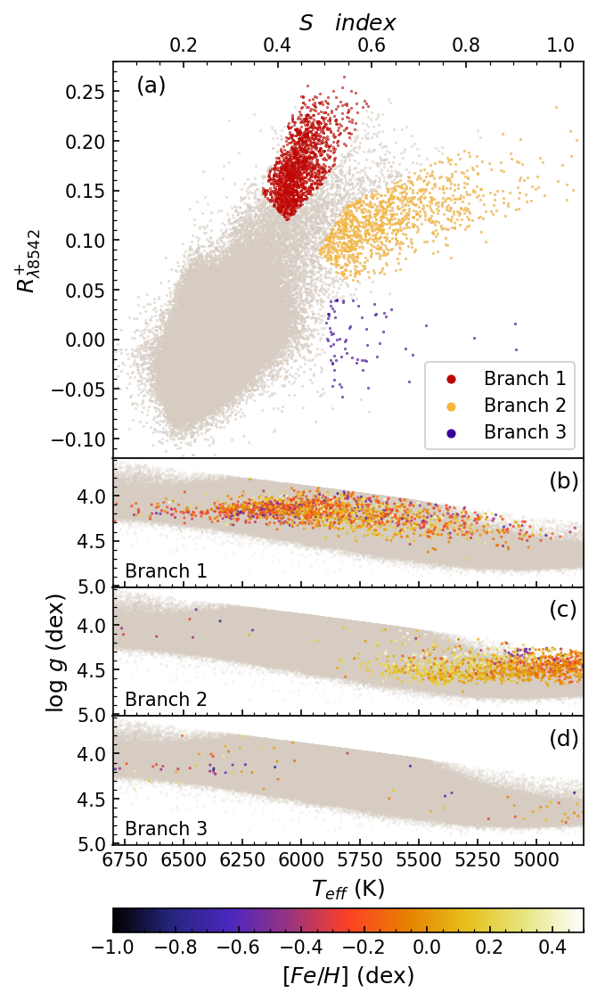
Figure 10: (a): Distribution of $S$ - $R^{+}_{\lambda 8542}$, different branches are defined by eyes and plotted in different color,as indicated in the frame. The background stars are shown in grey. (b): Distribution of Branch 1 stars in stellar parameter space. Metallicity is indicated by color, as shown in the bottom color bar, (c): Distribution of Branch 2 stars. (d): Distribution of Branch 3 stars.

To investigate the properties of the 3 groups, we check the spectra by eyes, the typical spectra are show in Figure 11.

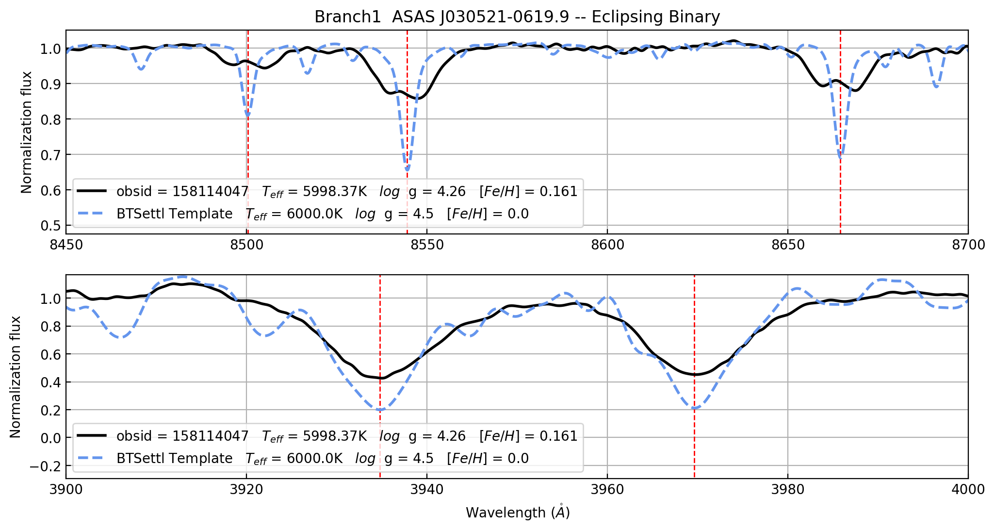
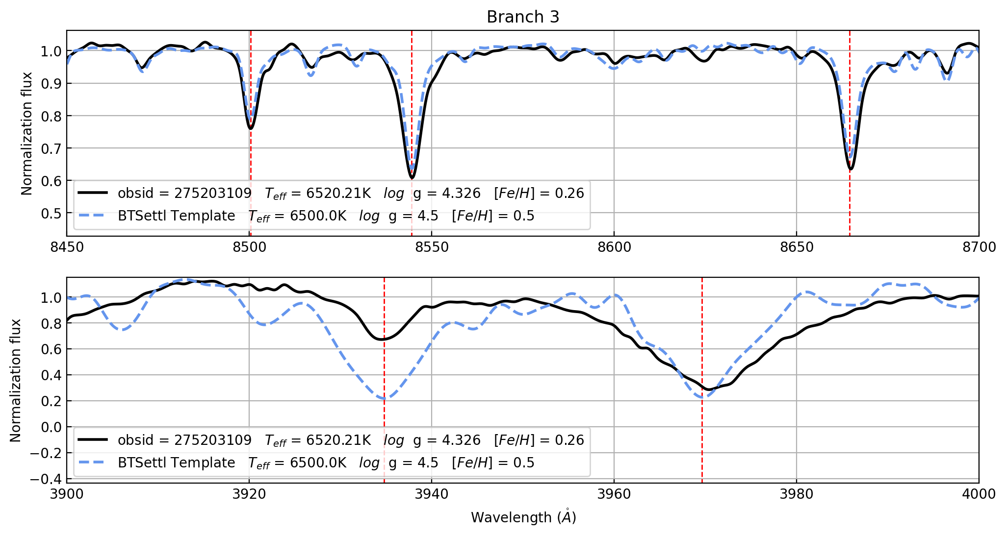
Figure 11: The typical spectra from the 3 branch star in Figure 10. From top to bottom are a star of Branch 1,2 and 3 respectively. The spectra and the corresponding template of the Ca II IRT region and the Ca II H&K region are plotted respectively.

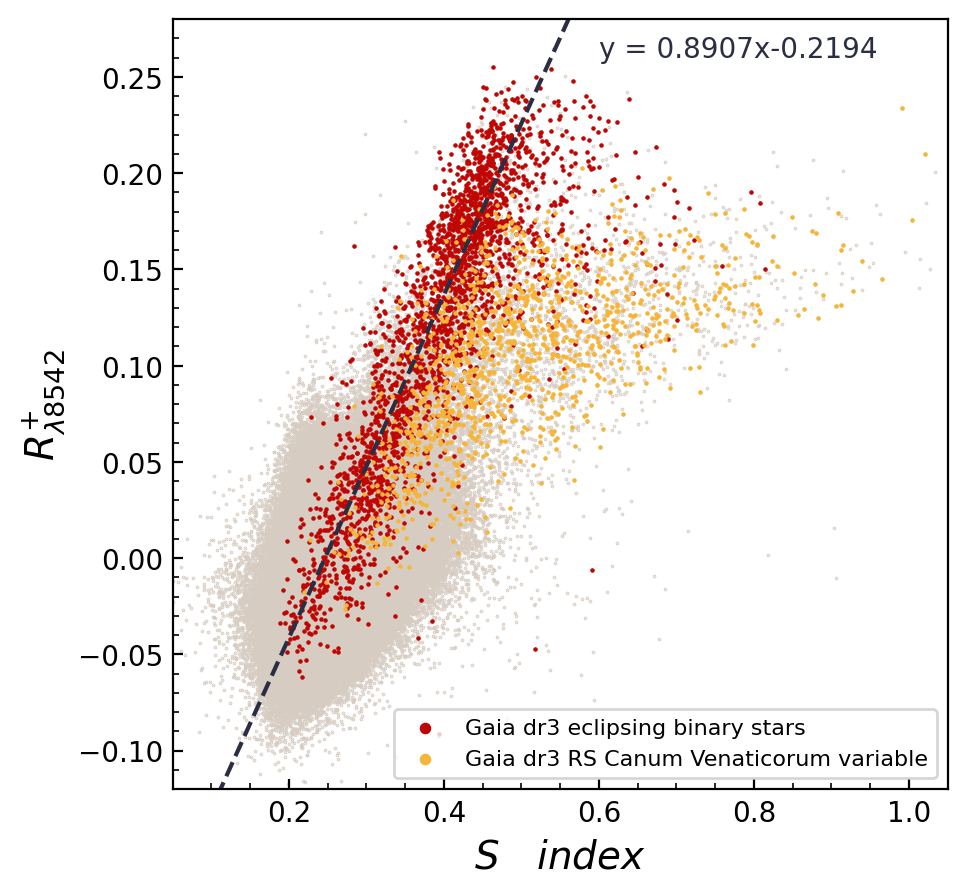
Figure 12: $R^{+}_{\lambda 8542}$ VS $S$ index distribution. The background grey points are the same as Figure 9. Overlaid color samples are stars cross matched with gaia dr3 eclipsing binaries and RS-CVn stars, respectively, as indicated in the figure. Those two samples are coincident with Brach 1 and Brach 2 defined in Figure 10, respectively. The black dash line is the linear regression of the eclipsing binary sample, the function is marked in the upper right corner.

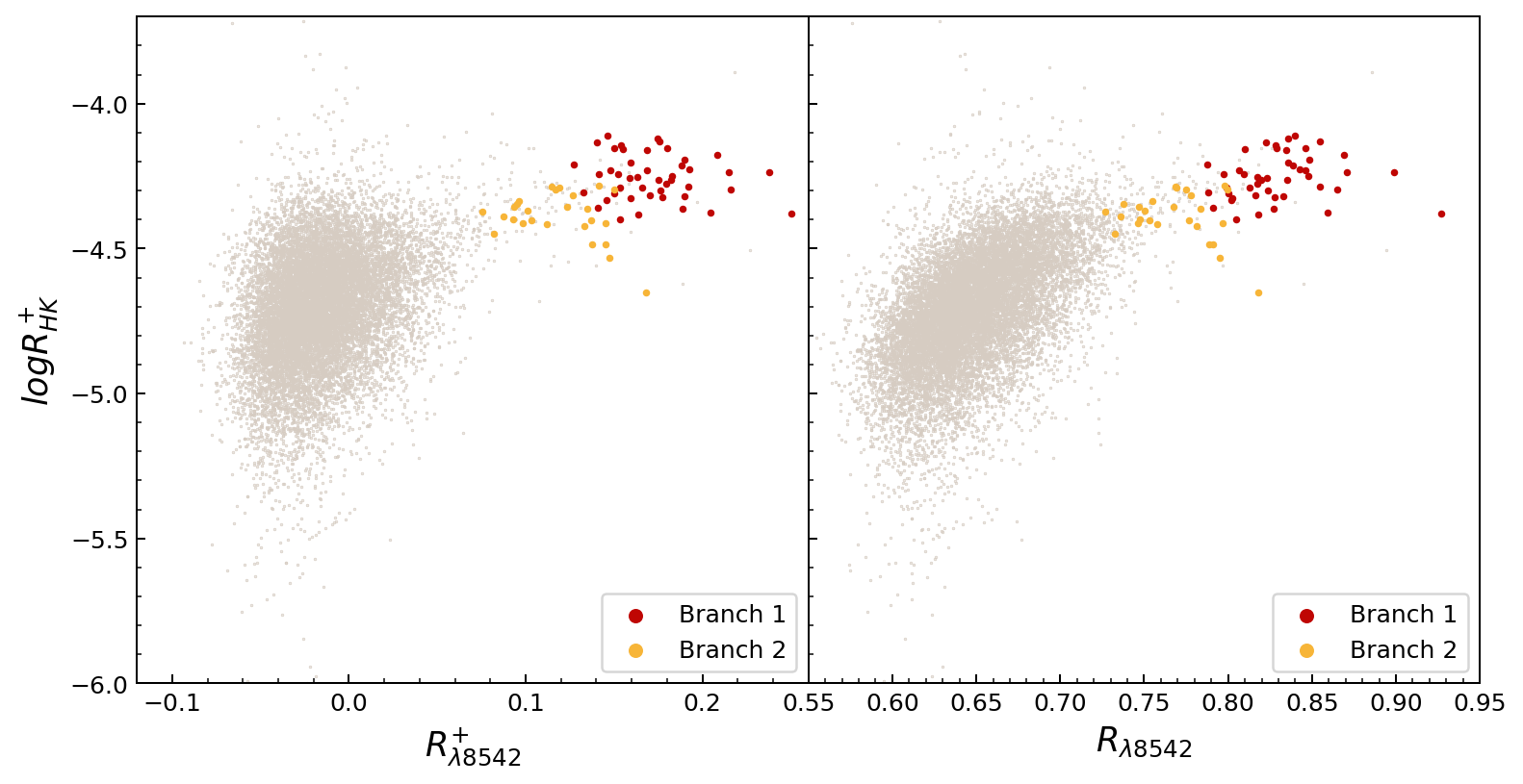
Figure 13: left panel: Relationship of $R^{+}_{\lambda 8542}$ - $logR^{+}_{HK}$. right panel: Relationship of $R_{\lambda 8542}$ - $logR^{+}_{HK}$. Red and yellow points are stars of Branch 1 and 2 defined in 10, respectively.

1. Most of the spectra in Branch 1 show character of double lines at IRT band and H&K lines are broader than the template, which is typical in spectral binaries. For LAMOST low resolution spectra, the radial velocity separation should be more than 150km/s for the 2 lines to be clearly discerned. So those are highly possible to be close binaries with larger RV difference and similar luminosity. To confirm this conclusion, we cross-match the samples with the gaiadr3.vari_eclipsing_binary catalog (Gaia et al., 2016; Vallenari et al., 2023; Mowlavi et al., 2023), which yielded 1727 common spectra (1507 common sources). About 66% (997/1507) stars in our defined Branch 1 region(Figure 10) are coincident with the Gaia dr3 eclipsing binaries. As the Gaia samples are selected by light curves thus are highly dependent on the inclination angle, the rest 34% of Branch 1 are either spectral binaries of low inclination that show no eclipse in lightcurve, or possibly some single stars show real high activity. So a large fraction of this branch should be close binaries mimic the chromospheric emission due to the index calculation algorithm, most of them are not active stars, or at least not as high as the $S$ or $R$ index indicated. Further investigation is necessary to determine their nature. The Gaia eclipsing binary sampleS extend linearly to the low active index end in the $S$ vs $R^{+}$ plot (Figure 12). We fitted the Gaia samples with RANSAC (Random Sample Consensus) regression algorithm provided by sklearn package (Pedregosa et al., 2011), the result is shown in Figure 12.

2. For Branch 2, we observed obvious emission cores in most of the spectra at the $H\&K$ lines, and filled-in core of the Ca II IRT absorption lines. So the branch 2 is dominated by highly chromospheric activity stars. From the parameters distribution, they are predominantly metal rich (i.e. $[Fe/H]>-0.2$) cool stars ($T_{eff}<5700K$). As RS Canum Venaticorum variable (RS-CVn) is a type of chromospheric active binaries, we crossed correlate our catalog with the Gaia RS-CVn catalog (Rimoldini et al., 2023), and got 1187 spectra (1037 stars) in common. The matched Gaia RS-CVns are plotted in Figure 12, most of these stars are consistent with Branch 2 and exhibit clear differences from eclipsing binaries.

3. Branch 3 shows higher $S$ index and relatively lower $R^{+}$ index, which means the H&K lines show higher activity than IRT lines. We suspect this may be caused by binaries or visually close stars with different temperature, the blue and red region are dominated by different star that falling into the same fiber. Since there are only 70 stars in this category, those stars were checked one by one. Miscellaneous informations such as CDS (http://cdsportal.u-strasbg.fr/) images, SED, LAMOST spectra, Gaia non-single star list (Holl et al., 2023), TESS light curves (Ricker et al., 2015; Sullivan et al., 2015) and Kepler light curves (Howell et al., 2014) were collected to help to understand the nature of these targets, those information are listed in the last column of Table LABEL:tabA1. From the table, 21 of them are binaries or spacial coincidence, supporting our speculation. 27 of them are variables that may show high activity, 10 of them have no particular reason and the rest of them are due to pollution or are with wrong spectral type, further study is necessary to know their nature.

5.3 Comparing with $R^{+}_{HK}$index

Using the $logR^{+}_{HK}$ index in Zhang et al. (2020) (Table 1), the distribution of $R^{+}_{\lambda 8542}$ - $logR^{+}_{HK}$ and $R_{\lambda 8542}$ - $logR^{+}_{HK}$ were plotted in Figure 13. The stars in Branch 1 and Branch 2 in previous section are also plotted. The overall distribution is similar to Žerjal et al. (see 2013, Fig.7), though they used $EW_{IRT}$ as infrared activity indicator. Binary stars are more likely to appear in the region of both high H&K and high IRT index, similar to Žerjal et al. (2013). From Fig 12 and 13, high H&K or high IRT index alone is not a good indicator of activity as there is a large population of binaries with low stellar activity mimic the high activity star. Combing the H&K index and the IRT index, especially in the S vs $R^{+}_{\lambda 8542}$ distribution plot, will be more helpful to decern different population of stellar activity.

6 Conclusion

We defined new infrared Ca II triplet stellar activity indices, $R$ and $R^{+}$, and derived the indices for 699,348 spectra of 562,863 solar like F, G and K-type stars. These activity indices, as well as their estimated uncertainties and other basic information are integrated in a database available at https://nadc.china-vo.org/res/r101246/.

Comparing the indices of $\lambda 8498$, $\lambda 8542$ and $\lambda 8662$ lines, they show linear correlation in each pairs. The $R^{+}_{\lambda 8542}$ is the strongest among the three lines, and could be used as the indicator to represent the Ca II IRT activity. We presented the distribution of $\lambda 8542$ index in stellar parameter space, and selected samples of high active and low active stars, respectively. The fraction of low active stars decrease with the temperature, well the fraction of high active stars first decrease with the temperature above 5800K, then below 5800K, the fraction increase with the decreasing temperature. We further compare our infrared activity index with the Ca II H&K index and find that the high $S$ index star could be divide into 3 branches, Branch 1 are mostly spectral binaries with double lines that mimic the emission line core, Branch 2 are RS CVns that show high activity, Brach 3 are stars show high $S$ index but relatively low $R^{+}_{\lambda 8542}$ index due to difference reasons. Combining the CaII H&K $S$ index and $R^{+}_{\lambda 8542}$ is particularly useful in selecting true chromospheric active stars. A future work is necessary to exclude pollution from low active binaries and establish a pure sample of high active stars.

Appendix A List of Branch 3 stars

Table A1: Information of stars in Branch3

No.	obsid	gaia_source_id	g_mag	ra_obs	dec_obs	$R^{+}_{8542}$	S Index	Class
1	181415234	2742433723412879360	13.07488	1.883999	5.700471	0.023102	0.62965	*UV excess/binary?
2	255415044	390549008386598016	14.26488	11.21287	48.28147	0.035161	0.604901	*Bright Star Pollution
3	182715182	376725089206420864	14.22984	16.69563	44.43003	0.01305	0.554792	Variable (G)
4	209103032	114150201980200960	12.09423	40.99757	24.91994	-0.02086	0.585086	*Nearby Star Pollution
5	162403203	108894639478505472	13.62411	46.7181	22.2539	0.015495	0.903646	*Young Stellar Object Candidate
6	157302145	125962495916228992	12.85282	50.73753	34.37201	-0.00395	0.61698	Variable(G)
7	286103110	67691055407537792	13.16509	53.43127	23.15588	-0.01764	0.610353	Binary (G)
8	307915107	3250965204243797760	12.7828	55.21712	-1.54672	-0.01576	0.685768	*Visual Binary
9	111607167	70286319462343808	11.74727	56.30801	26.5884	0.038976	0.525731	Variable(G)
10	480603181	65205166993246080	14.21742	56.58174	23.91762	-0.04815	0.534726	*Bright Star Pollution
11	100904105	65223618172733952	11.95708	56.6641	24.02969	0.037559	0.539393	*BY Dra Variable
12	204105048	163600634362268800	11.44613	60.13293	27.42786	0.031089	0.515465	*MS+WD Binary
13	273916194	232362820257069440	10.37425	62.41018	43.59254	-0.0312	0.581389	Variable(K)
14	470205184	232914736434443136	14.58639	64.16136	45.60959	-0.05821	0.536967
15	384509039	3285027799594151680	13.08165	65.08137	5.838964	0.039738	0.526472	Variable(K)
16	275203109	253742995657660288	10.77930	67.0192	45.56416	-0.04711	0.517125	Binary (G)
17	361716215	277067485569047680	11.67850	67.28308	55.21747	-0.00102	0.505846	Variable(K)
18	250801006	3405685422487373568	14.17399	73.94313	17.28189	0.039493	0.537972	Variable (G)
19	39104099	205354966385794048	12.32107	73.95885	43.69652	-0.04074	0.520087	Variable(K)
20	528007141	3228908790535918976	14.17989	75.26918	1.364525	0.000329	0.53148	Variable(G)
21	307304141	211681178338056192	12.04812	78.64506	45.42125	-0.04892	0.592449	Variable(K)
22	678513097	281149010170791552	14.78009	79.71296	59.046	0.005221	0.513852	Variable(G)
23	89713095	3448967285402131712	12.44196	82.39802	32.74561	0.028367	0.520001	*Nearby Star Pollution
24	208806168	3333163830247192064	12.34049	84.0461	6.520935	0.005564	0.517577	Variable(K)
25	393309119	3397615659976935296	11.66793	84.67204	18.00152	-0.02442	0.516078
26	505215137	3216524342533541248	15.34401	85.14597	-2.19503	0.013964	0.715127	*Nebula Pollution
27	505204206	3216417655546088192	15.33606	85.17643	-2.84414	-0.04222	0.678071	*Nebula Pollution
28	297011180	189407787175600640	11.11371	85.21744	37.46183	-0.00455	0.518133	Variable(K)
29	505215105	3216425077249628544	14.59378	85.24724	-2.74513	-0.02399	0.567592	*Nebula Pollution
30	547505087	3399231147498442112	11.37671	85.84326	19.40144	-0.00609	0.590741	*Eclipsing Binary
31	127806031	3431388156057648128	11.96078	90.89316	28.81194	-0.02395	0.516935	*Chemically Peculiar Star/Nearby star Pollution
32	486302167	3423621618233438080	14.50957	90.98312	21.90916	-0.03055	0.52059
33	606202112	3375271831352365568	13.13685	91.74336	21.03054	0.033773	0.512433	Variable(K)
34	501916045	3328461188953301120	14.17653	91.90313	8.044743	0.011596	0.510486
35	641111226	3345719467060096768	15.06539	92.92255	15.19583	0.024583	0.606389
36	606211049	3426827038226866176	13.94504	93.65705	25.50473	-0.00978	0.542015	*RR Lyrae Variable
37	486809137	3425551463001195008	11.62234	94.2737	23.42387	0.02181	0.579099	Variable(K)
38	267811169	3370935975970328192	14.46051	95.64267	19.2116	-0.0069	0.512879
39	696613240	3102733650797714816	12.25146	103.3226	-3.61788	-0.045	0.531789	Giants with wrong logg (L)
40	378105061	993779054893891840	12.59996	104.1611	54.1417	0.038976	0.560594	Variable(K)
41	88605186	3109933798391183232	12.26119	110.448	-1.2325	0.039448	0.521697	Variable(K)
42	88805176	3109936826350414592	10.76796	110.5126	-1.13856	-0.02079	0.512853	*Spectral Binary
43	226703189	892715622559710592	14.19901	113.7437	33.00618	0.016696	0.503644	*MS+WD Binary
44	93609075	3064639245085801344	12.01463	123.5568	-5.45447	-0.00035	0.525129	*Visual Binary/Variable(K)
45	308415140	3098139547613310720	12.97677	124.1939	8.390326	0.033797	0.570646	Variable(K)
46	656613008	636182586087691392	14.07274	136.9056	18.83429	-0.01988	0.569886
47	201907064	3824325436834913920	11.80175	146.0101	-4.58495	0.025776	0.508454	Variable(G)
48	303015088	830588577026980992	11.67706	160.1215	46.73302	0.011674	0.552609	*High Proper Motion Star
49	401214096	3816910296057695232	12.01111	168.8487	5.573148	0.021652	0.521994	SB1 (L)
50	208509165	3695446967363569408	12.37765	188.6458	-1.01727	0.007846	0.51159	*Visual Binary
51	132212074	3650688086675908352	12.20117	221.798	-0.49315	0.029954	0.641464	*Hot Subdwarf
52	426805127	1597737184257054720	12.58121	233.8434	53.58372	0.001588	0.81768	Variable(K)
53	152601123	1353107529388288896	13.30084	252.5303	40.17427	-0.04238	1.122254	Cosmic Ray Pollution(L)
54	334701053	1360809745779585152	12.16614	262.6004	44.48631	0.025941	0.5065	Variable(K)
55	574714131	2133632795086109440	14.42111	286.6875	50.6358	-0.01803	0.558479
56	243012154	2102151990479456128	12.88417	287.9217	41.05147	-0.00226	0.542695	*Nearby Star pollution
57	369703082	2099502579773618560	12.64614	289.1561	39.14371	0.000118	0.505672	*Visual Binary
58	52403133	2101074331648268032	13.70564	290.483	39.73531	-0.01383	0.546077
59	580505166	2052645379929910144	13.74717	290.9112	38.33558	0.023596	0.509367	Variable(G)
60	362811058	2134979074057185408	13.58594	295.6626	50.14518	0.03832	0.512928	*Rotating Variable/Visual binary
61	355104179	2079247720169124992	14.78923	299.1187	45.4898	0.007736	0.623634	*Pulsating Variable
62	158908013	2082103770340838144	13.23867	300.7669	44.86653	-0.02103	0.578636	*Rotating Variable
63	260702136	2068072279678698112	13.12818	306.8594	41.61058	0.010496	0.588413	*Nearby Star Pollution? Variable(G)
64	587915134	2163026176885565568	14.99146	314.1843	44.80388	-0.00931	0.670712	*Nebula Pollution
65	169005207	1781458323057855360	12.24709	331.3152	20.28735	0.026222	0.625867	*Visual Binary
66	75308136	2735568299794226304	11.86591	335.6045	15.65098	-0.00043	0.544412	*Visual Binary
67	75308129	2735577375059931264	12.50423	335.722	15.78769	-0.01789	0.535658
68	270405145	2008973392251158784	14.50971	345.2708	55.97517	-0.02235	0.587842	*Nearby Star Pollution
69	387904014	2664836171318493696	14.05540	349.4505	7.379211	0.025358	0.609652	*Hot Subdwarf Candidate / UV excess
70	180206182	1924190810839989632	12.92156	350.0968	40.73101	-0.0105	0.905189	*Visual Binary

References

- Allard et al. (1997) Allard, F., Hauschildt, P. H., Alexander, D. R., & Starrfield, S. 1997, ARA&A, 35, 137
- Allard et al. (2011) Allard, F., Homeier, D., & Freytag, B. 2011, in 16th Cambridge Workshop on Cool Stars, Stellar Systems, and the Sun, Vol. 448, 91
- Allard et al. (2013) Allard, F., Homeier, D., Freytag, B., Schaffenberger, W., & Rajpurohit, A. 2013, Memorie della Societa Astronomica Italiana Supplementi, 24, 128
- Andretta et al. (2005) Andretta, V., Busà, I., Gomez, M., & Terranegra, L. 2005, A&A, 430, 669
- Bai et al. (2017) Bai, Z.-R., Zhang, H.-T., Yuan, H.-L., et al. 2017, Research in Astronomy and Astrophysics, 17, 091
- Bai et al. (2021) —. 2021, Research in Astronomy and Astrophysics, 21, 249
- Bercik et al. (2005) Bercik, D., Fisher, G., Johns-Krull, C., & Abbett, W. 2005, ApJ, 631, 529
- Brasseur et al. (2019) Brasseur, C., Phillip, C., Fleming, S. W., Mullally, S., & White, R. L. 2019, Astrophysics Source Code Library, ascl
- Cauzzi et al. (2008) Cauzzi, G., Reardon, K., Uitenbroek, H., et al. 2008, A&A, 480, 515
- Cincunegui et al. (2007) Cincunegui, C., Diaz, R. F., & Mauas, P. J. D. 2007, A&A, 469, 309
- de Grijs & Kamath (2021) de Grijs, R., & Kamath, D. 2021, Universe, 7, 440
- Gaia et al. (2016) Gaia, C., Bono, G., et al. 2016, A&A, 595, 1
- Gentile Fusillo et al. (2015) Gentile Fusillo, N., Rebassa-Mansergas, A., Gänsicke, B., et al. 2015, MNRAS, 452, 765
- Ginsburg et al. (2019) Ginsburg, A., Sipőcz, B. M., Brasseur, C. E., et al. 2019, AJ, 157, 98, doi: 10.3847/1538-3881/aafc33
- Harris et al. (2020) Harris, C. R., Millman, K. J., van der Walt, S. J., et al. 2020, Nature, 585, 357, doi: 10.1038/s41586-020-2649-2
- He et al. (2023) He, H., Zhang, W., Zhang, H., et al. 2023, Ap&SS, 368, 63
- Hojjatpanah et al. (2020) Hojjatpanah, S., Oshagh, M., Figueira, P., Santos, N., & Amazo-Gómez, E. 2020, A&A, 439, A35
- Holl et al. (2023) Holl, B., Sozzetti, A., Sahlmann, J., et al. 2023, A&A, 674, A10, doi: 10.1051/0004-6361/202244161
- Howard et al. (2018) Howard, W. S., Tilley, M. A., Corbett, H., et al. 2018, ApJ, 860, L30
- Howell et al. (2014) Howell, S. B., Sobeck, C., Haas, M., et al. 2014, PASP, 126, 398
- Hunter (2007) Hunter, J. D. 2007, Computing in Science & Engineering, 9, 90, doi: 10.1109/MCSE.2007.55
- Husser et al. (2013) Husser, T.-O., Wende-von Berg, S., Dreizler, S., et al. 2013, A&A, 553, A6
- Karoff et al. (2016) Karoff, C., Knudsen, M. F., De Cat, P., et al. 2016, Nature Communications, 7, 11058
- Korhonen et al. (2015) Korhonen, H., Andersen, J., Piskunov, N., Hackman, T., & Juncher, D. 2015, MNRAS, 448, 3038
- Lanzafame et al. (2023) Lanzafame, A. C., Brugaletta, E., Frémat, Y., et al. 2023, A&A, 674, A30, doi: 10.1051/0004-6361/202244156
- Lightkurve Collaboration et al. (2018) Lightkurve Collaboration, Cardoso, J. V. d. M., Hedges, C., et al. 2018, Lightkurve: Kepler and TESS time series analysis in Python, Astrophysics Source Code Library. http://ascl.net/1812.013
- Lillo-Box et al. (2022) Lillo-Box, J., Santos, N., Santerne, A., et al. 2022, A&A, 667, A102
- Linsky et al. (1979) Linsky, J. L., Worden, S., McClintock, W., & Robertson, R. M. 1979, ApJS, 41, 47
- Martin et al. (2017) Martin, J., Fuhrmeister, B., Mittag, M., et al. 2017, A&A, 605, A113
- Mittag et al. (2019) Mittag, M., Schmitt, J., Metcalfe, T., Hempelmann, A., & Schröder, K.-P. 2019, A&A, 628, A107
- Mittag et al. (2013) Mittag, M., Schmitt, J., & Schröder, K.-P. 2013, A&A, 549, A117
- Mowlavi et al. (2023) Mowlavi, N., Holl, B., Lecoeur-Taïbi, I., et al. 2023, A&A, 674, A16
- Mullan (1979) Mullan, D. 1979, ApJ, 234, 579
- Notsu et al. (2015) Notsu, Y., Honda, S., Maehara, H., et al. 2015, PASJ, 67, 33
- Pedregosa et al. (2011) Pedregosa, F., Varoquaux, G., Gramfort, A., et al. 2011, Journal of Machine Learning Research, 12, 2825
- Price-Whelan et al. (2018) Price-Whelan, A. M., Sipőcz, B., Günther, H., et al. 2018, AJ, 156, 123
- Price-Whelan et al. (2022) Price-Whelan, A. M., Lim, P. L., Earl, N., et al. 2022, ApJ, 935, 167
- Ren et al. (2020) Ren, J.-J., Raddi, R., Rebassa-Mansergas, A., et al. 2020, ApJ, 905, 38
- Ricker et al. (2015) Ricker, G. R., Winn, J. N., Vanderspek, R., et al. 2015, Journal of Astronomical Telescopes, Instruments, and Systems, 1, 014003
- Rimoldini et al. (2023) Rimoldini, L., Holl, B., Gavras, P., et al. 2023, A&A, 674, A14
- Robitaille et al. (2013) Robitaille, T. P., Tollerud, E. J., Greenfield, P., et al. 2013, A&A, 558, A33
- Schrijver et al. (1989) Schrijver, C. J., Cote, J., Zwaan, C., & Saar, S. H. 1989, ApJ, 337, 964
- Shields et al. (2016) Shields, A. L., Ballard, S., & Johnson, J. A. 2016, Phys. Rep., 663, 1
- Sullivan et al. (2015) Sullivan, P. W., Winn, J. N., Berta-Thompson, Z. K., et al. 2015, ApJ, 809, 77
- Taylor (2005) Taylor, M. B. 2005, in Astronomical Society of the Pacific Conference Series, Vol. 347, Astronomical Data Analysis Software and Systems XIV, ed. P. Shopbell, M. Britton, & R. Ebert, 29
- Tennyson (2019) Tennyson, J. 2019, Astronomical Spectroscopy: An Introduction to the Atomic and Molecular Physics of Astronomical Spectroscopy (World Scientific)
- Vallenari et al. (2023) Vallenari, A., Brown, A., Prusti, T., et al. 2023, Astronomy & Astrophysics, 674, A1
- Virtanen et al. (2020) Virtanen, P., Gommers, R., Oliphant, T. E., et al. 2020, Nature Methods, 17, 261, doi: 10.1038/s41592-019-0686-2
- Wilson (1968) Wilson, O. 1968, ApJ, 153, 221
- Wright (2005) Wright, J. 2005, PASP, 117, 657
- Wu et al. (2011) Wu, Y., Luo, A.-L., Li, H.-N., et al. 2011, Research in Astronomy and Astrophysics, 11, 924
- Žerjal et al. (2013) Žerjal, M., Zwitter, T., Matijevič, G., et al. 2013, ApJ, 776, 127
- Zhang et al. (2019) Zhang, J., Zhao, J., Oswalt, T. D., et al. 2019, ApJ, 887, 84
- Zhang et al. (2020) Zhang, J., Bi, S., Li, Y., et al. 2020, ApJS, 247, 9
- Zhang et al. (2022) Zhang, W., Zhang, J., He, H., et al. 2022, ApJS, 263, 12
- Zhao et al. (2012) Zhao, G., Zhao, Y.-H., Chu, Y.-Q., Jing, Y.-P., & Deng, L.-C. 2012, Research in Astronomy and Astrophysics, 12, 723