Resolution enhancement, noise suppression, and joint T2* decay estimation in dual-echo sodium-23 MR imaging using anatomically-guided reconstruction

Abstract

Purpose: Sodium MRI is challenging because of the low tissue concentration of the ²³Na nucleus and its extremely fast biexponential transverse relaxation rate. In this article, we present an iterative reconstruction framework using dual-echo ²³Na data and exploiting anatomical prior information (AGR) from high-resolution, low-noise, ¹H MR images. This framework enables the estimation and modeling of the spatially-varying signal decay due to transverse relaxation during readout (AGRdm), which leads to images of better resolution and reduced noise resulting in improved quantification of the reconstructed ²³Na images.

Methods: The proposed framework was evaluated using reconstructions of 30 noise realizations of realistic simulations of dual echo twisted projection imaging (TPI) ²³Na data. Moreover, three dual echo ²³Na TPI brain data sets of healthy controls acquired on a 3T Siemens Prisma system were reconstructed using conventional reconstruction, AGR and AGRdm.

Results: Our simulations show that compared to conventional reconstructions, AGR and AGRdm show improved bias-noise characteristics in several regions of the brain. Moreover, AGR and AGRdm images show more anatomical detail and less noise in the reconstructions of the experimental data sets. Compared to AGR and the conventional reconstruction, AGRdm shows higher contrast in the sodium concentration ratio between gray and white matter and between gray matter and the brain stem.

Conclusion: AGR and AGRdm generate ²³Na images with high resolution, high levels of anatomical detail, and low levels of noise, potentially enabling high-quality ²³Na MR imaging at 3T.

Accepted for publication in Magnetic Resonance in Medicine on 04 Nov 2023.

1 Introduction

Sodium-23 (²³Na) is the second most abundant MR-active nucleus in the human body and plays a crucial role in ion homeostasis and cell viability. Changes in tissue sodium concentration have been shown to provide physiologically relevant information for challenging brain pathologies such such as brain tumors [1, 2], stroke [3, 4] and Alzheimer’s disease [5, 6, 7]. For an in-depth overview on the state-of-the-art of in vivo MR sodium imaging techniques and applications, we refer to the recent reviews by Madelin [8], Sha [9], Thulborn [10] and Hagiwara [11]. Despite its unique potential for providing non-invasive and physiologically relevant information, the development and clinical acceptance of sodium MRI has been hampered compared to proton MRI, owing to the unique data acquisition challenges posed by the NMR properties of the ²³Na nucleus, namely:

1. lower NMR sensitivity, due to its 4x lower gyromagnetic ratio

2. (ca. 2000x) lower tissue concentration

3. very short (biexponential) transverse ($T_{2}^{*}$) relaxation.

The combination of the latter two properties limits the maximum k-space frequency $k_{\text{max}}$ that can be used for acquiring images of adequate signal-to-noise ratio (SNR) in clinically practical imaging times (ca. 10 min). Moreover, the images that are commonly obtained, suffer from spatial blurring beyond that corresponding to the nominal spatial resolution of the acquired spatial frequency values (i.e., $1/2k_{\text{max}}$) due to the fast decay of the signal during readout. As discussed in [12, 7], a direct consequence of the rather low resolution of sodium images are severe partial volume effects (PVEs) that make accurate quantification of local sodium concentration difficult. This is especially the case, when changes in local sodium concentration in the brain are accompanied by atrophy, necessitating advanced methods for partial volume correction.

In layman’s terms, one could say that compared to standard proton MR images, due to the unfavorable NMR properties of ²³Na, sodium MR images are “blurry” and “noisy” - similar to images acquired in emission tomography (PET and SPECT). To simultaneously deblur and denoise emission tomography images, several reconstruction methods based on high-resolution and low-noise structural (anatomical) prior images have been proposed over the last 30 years; see, e.g. [13, 14, 15, 16, 17, 18, 19, 20]. Similar methods have been applied in proton MR imaging in the context of spectroscopic imaging [21], extended k-space sampling [22] and undersampled multicontrast MR reconstruction [23]. In ²³Na MR reconstruction, Gnahm et al. proposed to include structural prior information from various proton MR contrasts using a anatomically-weighted first and second order total variation (AnaWeTV) [24]. Based on reconstructions of simulated and real data, and in agreement with the results obtained in articles on structure-guided reconstruction in emission tomography, the authors conclude that “The approach (AnaWeTV) leads to significantly increased SNR and enhanced resolution of known structures in the images … Therefore, the AnaWeTV algorithm is in particular beneficial for the evaluation of tissue structures that are visible in both ²³Na and ¹H MRI.” In 2021, Zhao et al. [25] proposed a reconstruction method based on a motion compensated generalized series model and a sparse model where anatomical prior information from a segmented high-resolution proton image was used for denoising and resolution enhancement. The authors also concluded that the proposed anatomically constrained reconstruction method substantially improved SNR and lesion fidelity.

In this work, we propose using anatomical guidance based on the segmentation-free directional total variation (dTV) prior not only for denoising and resolution enhancement of ²³Na images, but also for local signal decay estimation and compensation in a joint reconstruction framework for dual echo ²³Na acquisitions. In the context of multicontrast proton MRI reconstruction, Ehrhardt and Betcke [23] already showed that dTV is superior compared to AnaWeTV. Furthermore, in 2022 Ehrhardt et al. [26] showed that dTV is a promising prior for denoising and resolution enhancement of hyperpolarized carbon-13 MRI, which motivated us to also use dTV for the reconstruction of dual echo sodium MR data.

The rest of the article is structured as follows: In the next section, we explain the theory behind dual echo ²³Na reconstruction, including local $T_{2}^{*}$ decay estimation and modeling, as well as anatomical guidance through directional total variation before evaluating our framework based on simulated and experimental data from healthy human volunteers.

2 Theory

2.1 Conventional iterative single-echo sodium MR image reconstruction

Assuming additive uniform Gaussian noise on the measured complex-valued (non-Cartesian) single-echo MR raw data $d\in\mathbb{C}^{m}$, we can define the conventional maximum a posteriori single echo data MR reconstruction problem via the optimization problem

$$\operatorname*{arg\,min}_{u}\Biggl{(}\frac{1}{2}\sum_{l=1}^{m}|F_{k(t_{l})}u-d_{l}|^{2}+\beta R(u)\Biggr{)}\ ,$$ (1)

with $u\in\mathbb{C}^{n}$ being the complex (sodium) MR image to be reconstructed, $R:\mathbb{C}^{n}\to\mathbb{R}$ being a regularization functional weighted by the real-valued scalar $\beta$. In (1) $|\cdot|$ denotes the absolute value of a complex number, and we define $F_{k(t)}:\mathbb{C}^{n}\to\mathbb{C}$ as the Fourier encoding operator mapping a complex-valued input image $w$ to a single point in k-space ($k_{x}(t)$,$k_{y}(t)$,$k_{z}(t)$) via

$$F_{k}w=\sum_{j=1}^{n}w_{j}\exp\Bigl{(}-i(k_{x}x_{j}+k_{y}y_{j}+k_{z}z_{j})\Bigr{)}\ ,$$ (2)

where ($x_{j}$,$y_{j}$,$z_{j}$) are the spatial coordinates of voxel $j$. Given a k-space readout trajectory $(k_{x}(t),k_{y}(t),k_{z}(t))$ as a function of time $t$, $F$ can be evaluated using the discrete-time Fourier transform or approximated by the non-uniform fast Fourier transform (NUFFT) [27]. Note that if the readout time is not short compared to the spatially-varying transverse relaxation times $T_{2}^{*}(x,y,z)$, k-space data points acquired “late” after excitation suffer from apodization caused by $T_{2}^{*}$ relaxation of the signal. For typical non-Cartesian readouts that move outwards starting at the center of k-space, that implies damping of the high frequency data points leading to a spatially-varying loss of resolution when optimizing (1).

2.2 Sodium MR reconstruction including transverse relaxation modeling

If the spatially-varying transverse relaxation is known, it can in principle be included in the forward model (1) to compensate for the added blurring caused by the transverse relaxation. Assuming a generic known transverse relaxation function $d(x,y,z,t)\to[0,1]$ (e.g. a multi-exponential decay) and ignoring the effects of main magnetic field inhomogeneities on the k-space trajectory [28, 29] because of sodium’s much lower gyromagnetic ratio, we can rewrite the Fourier forward model (1) into

$$\begin{split}\tilde{F}_{k(t_{l})}w=\sum_{j=1}^{n}&w_{j}\,d(x_{j},y_{j},z_{j},t_{l})\\ &\exp\Bigl{(}-i(k_{x}(t_{l})x_{j}+k_{y}(t_{l})y_{j}+k_{z}(t_{l})z_{j})\Bigr{)}.\end{split}$$ (3)

In case the transverse relaxation is modeled by an effective spatially-varying monoexponential decay, we obtain

$$\begin{split}\tilde{F}_{k(t_{l})}w=\sum_{j=1}^{n}&w_{j}\,\exp\Bigl{(}-\frac{t_{l}}{T_{2}^{*}(x_{j},y_{j},z_{j})}\Bigr{)}\\ &\exp\Bigl{(}-i(k_{x}(t_{l})x_{j}+k_{y}(t_{l})y_{j}+k_{z}(t_{l})z_{j})\Bigr{)}\ ,\end{split}$$ (4)

where $T_{2}^{*}(x_{j},y_{j},z_{j})$ denotes the effective monoexponential transverse relaxation time at voxel $j$. Note, however, that in practice the transverse relaxation function $d(x,y,z,t)$ is unknown, since it depends, among other things, on the type of tissue and inhomogeneities of the field $B_{0}$.

One way to obtain information about the transverse relaxation function $d$ is to perform multiple acquisitions at different echo times. A “naive” way to extract $d$ would be to independently reconstruct all data sets by optimizing (1) followed by a voxel-wise fit of the decay model. However, this approach is severely hampered by the inherent low SNR of the sodium MR signal and the finite time available for data acquisition.

As a better alternative, we propose to jointly estimate a simplified spatially-varying decay model during reconstruction of dual-echo data, as explained in the next section.

2.3 Dual-echo sodium MR image reconstruction including joint T2* estimation

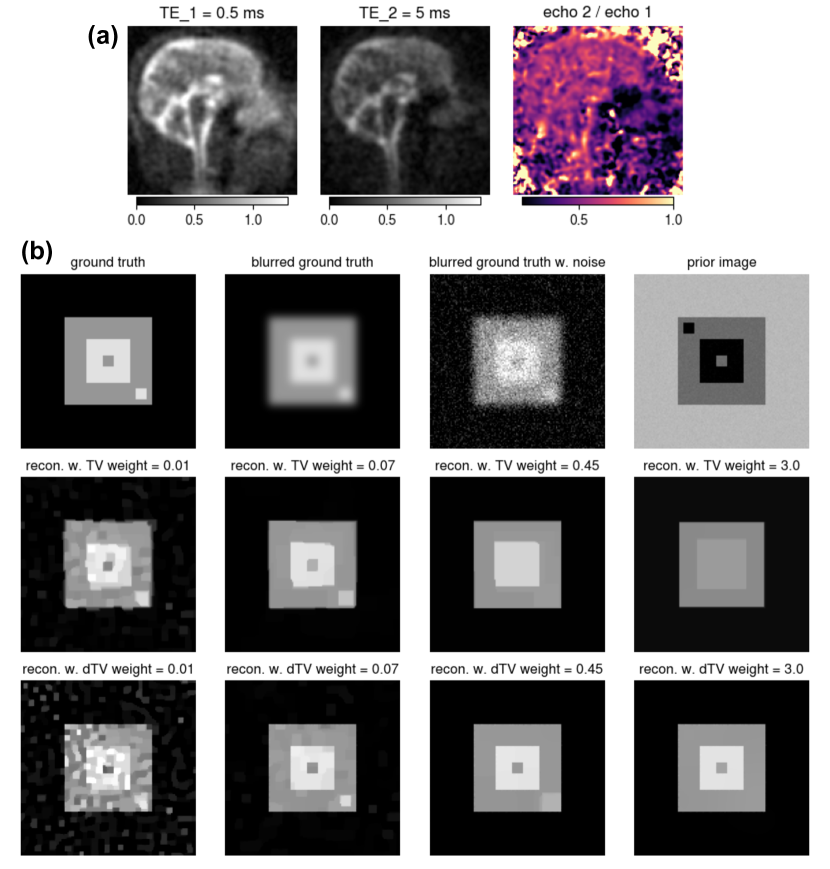
Figure 1: (a) (left): sagittal slice of ²³Na twisted projection imaging (TPI) acquisition with $T_{E1}$ = 0.5 ms (middle): same as left with $T_{E2}$ = 5.0 ms (right) ratio between $T_{E2}$ and $T_{E1}$ image showing spatially-varying rapid (e.g. regions close to nasopharynx, oropharynx and deep paranasal sinuses) and slower (e.g. CSF in ventricles) $T_{2}^{*}$ relaxation. (b) Illustration of structure-guidance with directional TV applied to an image deblurring and denoising problem. (Top row) ground truth, blurred ground truth, blurred ground truth with added noise (data to be reconstructed), and structural prior image. (Middle row) reconstructions using total variation (TV) as regularizer. (Bottom row) reconstructions using directional TV (dTV) as regularizer. The level of regularization is increasing from left to right. In contrast to TV, dTV avoids smoothing across edges that are present in the prior image.

The availability of two sodium MR acquisitions of the same subject at different echo times (e.g. 0.5 ms and 5 ms) allows extracting information about the spatially-varying transverse relaxation as illustrated in 1(a). For convenience, we re-write the monoexponential decay model used in (4) into the power function

$$\exp\Bigl{(}-\frac{t_{l}}{T_{2}^{*}(x_{j},y_{j},z_{j})}\Bigr{)}=r(x_{j},y_{j},z_{y})^{\nicefrac{{t_{l}}}{{\Delta T_{E}}}}\ ,$$ (5)

where $\Delta T_{E}$ is the difference between the first and the second echo time and $r\in[0,1]^{n}$ being an exponential transformation of the spatially-varying effective monoexponential $T_{2}^{*}$ map defined via

$$r_{j}=\exp\Biggl{(}-\frac{\Delta T_{E}}{T_{2}^{*}(x_{j},y_{j},z_{j})}\Biggr{)}\ .$$ (6)

Combining the data fidelity terms of both readouts and using the mappings

$$A_{1,l}(r) =F_{k(t_{l})}\operatorname{diag}(r^{\nicefrac{{t_{l}}}{{\Delta T_{E}}}})$$ (7)

$$A_{2,l}(r) =F_{k(t_{l})}\operatorname{diag}(r^{\nicefrac{{t_{l}}}{{\Delta T_{E}}}+1})\ ,$$ (8)

leads to the following dual-echo reconstruction problem with joint decay estimation

$$(u^{\dagger},r^{\dagger})\in\operatorname*{arg\,min}_{u,r}\mathcal{L}(u,r)$$ (9)

$$\begin{split}\mathcal{L}(u,r)=\Biggl{(}&\frac{1}{2}\sum_{l=1}^{m}|A_{1,l}(r)u-d_{l}^{T_{E1}}|^{2}+\\ &\frac{1}{2}\sum_{l=1}^{m}|A_{2,l}(r)u-d_{l}^{T_{E2}}|^{2}+\\ &\beta_{u}R_{u}(u)+\beta_{r}R_{r}(r)+\chi_{(0,1]}(r)\Biggr{)}\ ,\end{split}$$ (10)

where $u\in\mathbb{C}^{n}$ is the complex sodium image to be reconstructed, $r\in\mathbb{R}^{n}$ is the real “ratio decay” image to be jointly estimated, $\chi_{(0,1]}$ is the characteristic function of the convex set $\{r\mid 0<r_{j}\leq 1\ \forall j\}$, and $d_{l}^{T_{E1}}$ and $d_{l}^{T_{E2}}$ denote the $l$-th data point acquired at readout time $t_{l}$ corresponding to the 3D k-space point $k_{l}=k(t_{l})=(k_{x}(t_{l}),k_{y}(t_{l}),k_{z}(t_{l}))$ defined by the k-space trajectory from the acquisitions using the first ($T_{E1}$) and second echo time ($T_{E1}+\Delta T_{E}$), respectively. Note that in this work, we approximate the biexponential transverse relaxation using an effective monoexponential because: (i) acquisitions at two echo times were available and (ii) fitting a biexponential is less stable even if data from more echo times would be available. We also assume that data are acquired using a single channel volume head coil with a constant coil sensitivity. However, an extension of the data fidelity terms to multi-channel coil data with known sensitivity maps is straightforward. Finally, $R_{u}:\mathbb{C}^{n}\to\mathbb{R}$ and $R_{r}:\mathbb{R}^{n}\to\mathbb{R}$ are regularization functionals that are needed since equation (9) is ill-posed because the acquired sodium MR raw data have low SNR, particularly at high spatial frequencies due to apodization caused by the fast transverse relaxation.

2.4 Structure-guided regularization via directional total variation

When reconstructing low-resolution data and assuming that the image to be reconstructed is structurally similar to a prior image with higher resolution, it is reasonable to use regularization functionals that incorporate structure-guided information. Over the last couple of years, many of those regularization functionals have been proposed - see, e.g. the review book chapter [30]. A simple but powerful example is “directional total variation“ (dTV) proposed in [23], which was already applied to the reconstruction of multicontrast proton MR [23] and also hyperpolarized carbon-13 MR [26]. dTV can be seen as a structural extension of standard total variation in the presence of a (high resolution and low noise) prior image $v$.

Total variation can be defined as

$$\text{TV}(u)=\sum_{j=1}^{n}|\nabla u_{j}|\ ,$$ (11)

where $\nabla$ is the three-dimensional gradient operator mapping from $\mathbb{C}^{n}$ to $\mathbb{C}^{3n}$. In other words, to compute $\text{TV}(u)$, we first evaluate the gradient operator applied to the image $u$ at every voxel $j$ (e.g., by using the finite forward differences in all three directions) which results in a three-element gradient vector for every voxel $j$. Subsequently, we calculate a norm of the gradient vector (e.g. the L1 or L2 norm) at every voxel and finally sum all norms.

Based on this definition, Ehrhardt et al. [23] defined directional total variation as

$$\text{dTV}(u)=\sum_{j=1}^{n}|P_{\xi_{j}}\nabla u_{j}|\ ,$$ (12)

where $P_{\xi_{n}}:\mathbb{C}^{3}\to\mathbb{C}^{3}$ is a projection operator defined via

$$P_{\xi_{j}}g=g-\langle\xi_{j},g\rangle\xi_{j}\ ,$$ (13)

and $\xi_{n}$ is a normalized gradient vector-field derived from a structural prior image $v$ via

$$\xi_{j}=\frac{\nabla v_{j}}{\sqrt{|\nabla v_{j}|^{2}+\eta^{2}}}\ ,$$ (14)

where $\eta$ is a scalar that determines whether a gradient is considered large or small. $\eta$ can be chosen based on the noise-level in the prior image $v$, such that gradients due to noise are suppressed. Note that in the limit case $|\nabla v_{j}|\to 0$ (locally flat prior image), dTV reduces to TV. In the other limit case $|\nabla v_{j}|\gg\eta$, $\xi_{j}=\nabla v_{j}/|\nabla v_{j}|$ and hence $|\xi_{j}|=1$, which means that $P_{\xi_{j}}$ applied to a gradient vector $g$ subtracts the component of $g$ that is parallel to $\xi_{j}$ from $g$, or in other words, results in the component of $g$ that is orthogonal to $\xi_{j}$. Hence, instead of penalizing the norm of the “complete” gradient vector as in TV, dTV “only” penalizes the norm of the components of the gradient vectors that are perpendicular to the vectors of the joint gradient field. Consequently, a parallel or anti-parallel orientation of the gradient of the image to be reconstructed relative to the gradient field from the prior image is encouraged, independently of the magnitude of the joint gradient field (provided that $|\nabla v_{j}|\gg\eta$). A simplified denoising and deblurring example illustrating the difference between using TV and the structure-guided dTV prior is shown in Fig. 1(b).

3 Methods

To investigate our proposed structure-guided sodium MR reconstruction framework, which includes joint signal decay estimation and modeling, we performed reconstructions of simulated and experimental data from healthy volunteers. In this section, we first describe the simulation setup and the acquisition and reconstruction of the experimental data, followed by a detailed explanation of our strategy and implementation to solve the large-scale optimization (reconstruction) problem (9).

3.1 Simulation experiments

The performance of the proposed sodium reconstruction framework was first investigated using data simulated based on the brainweb phantom [31]. A high-resolution ground truth sodium image was generated using the tissue class label images of the brainweb phantom (subject 54). Fixed total sodium concentrations as well as short and long biexponential $T_{2}^{*}$ times were assigned to each tissue class; see Tab. 1. A spherical white matter lesion without corresponding edges in the structural prior T1 image was added to the ground truth TSC image to investigate structural mismatches. Dual-echo k-space data ($T_{E1}=0.455\,\text{ms}$ and $T_{E2}=5\,\text{ms}$) including biexponential $T_{2}^{*}$ decay were simulated as a weighted sum of the forward models in equation (4) using the twisted projection imaging (TPI) readout described in the next section and the simulated short (60%) and long $T_{2}^{*}$ images (40%). Subsequently, uniform Gaussian noise, reflecting the SNR observed in real data, was added to the real and imaginary part of the simulated k-space data.

In total, 30 noise realizations were generated and reconstructed using the following settings:

1. “Conventional” reconstruction (CR) of the first echo data set by solving equation (1) using a smooth non-structural “quadratic difference” prior $R(u)=\|\nabla u\|_{2}^{2}$ and a forward model that neglects signal decay during readout. This reconstruction method is very similar to a (filtered) inverse Fourier transform reconstruction of gridded k-space data, but has the advantage of correctly weighting the noise in the data fidelity term.

2. “Anatomically-guided” reconstruction (AGR) of the first echo data set by solving equation (1) using the structural dTV prior $R_{u}(u)=\text{dTV}(u)$ and a forward model that neglects signal decay during readout. The joint normalized gradient field $\xi$ needed for dTV was derived from the high-resolution proton T1 image of the brainweb phantom.

3. “Anatomically-guided” reconstruction of the combined first and second echo data set including joint signal decay estimation and modeling (AGRdm) by solving equation (9) using the structural dTV prior and a monoexponential for signal decay during readout in (7) for $u$ and $r$.

To study the potential bias introduced by modeling the biexponential decay using a simplified and estimated monoexponential model, simulated noise-free data sets were also reconstructed with AGRdm using the known biexponential model and compared to AGRdm using the estimated monoexponential model and AGR without decay model. All reconstructions used a grid size of 128x128x128 and were run for various levels of regularization ($\beta_{u}$ and $\beta_{r}$). The quality of all reconstructions was assessed in terms of regional bias-noise curves evaluated in different anatomical regions of interest (ROIs) that were defined based on grey matter, white matter and CSF compartments of the brainweb phantom which were further subdivided based on a freesurfer segmentation of the brainweb T1 image. Regional bias was quantified by first calculating the regional mean value in each ROI, followed by averaging across all noise realizations and subtracting the known ground truth values. Regional noise was assessed by first calculating the voxel-wise standard deviation image across noise realizations, followed by regional averaging across each ROI. Moreover, regional reconstruction quality was assessed by calculating the root-mean-square error in each ROI for all reconstructions across all noise realizations. In addition, the mean effetive monoexponential $T_{2}^{*}$ times estimated with AGRdm were quantified in cortical grey matter, white matter and in the ventricles using the estimatated ratio images $r$ and Eq. (6).

	GM	WM	CSF	lesion
TSC (arb. units)	0.6	0.4	1.5	0.6
short $T_{2}^{*}$ (ms)	3	3	50	3
long $T_{2}^{*}$ (ms)	20	18	50	18

Table 1: Total sodium concentration (TSC), and short and long $T_{2}^{*}$ values for grey matter (GM), white matter (WM), and cerebrospinal fluid (CSF) used in brainweb-based data simulation.

3.2 In vivo experiments

In addition to the simulation experiments, sodium MR raw data of three healthy controls (60yr male, 65 yr female, 42yr female) acquired in a previous study approved by the local IRB (New York University Grossman School of Medicine) were reconstructed. In this study, two single-quantum sodium images with different echo times were acquired on a 3T Siemens Prisma scanner with a dual-tuned (¹H-²³Na) volume head coil (QED, Cleveland, OH) that was also used for shimming. A TPI sequence [32] was used for data collection. The TPI parameters were: rectangular RF pulse of 0.5 ms duration, flip angle 90^∘, field of view (FOV) 220 mm, matrix size 64, TPI readout time 36.32 ms, total number of TPI projections 1596, P = 0.4 (the fraction of $k_{\text{max}}$ where the transition from radial to twisted readout occurs), TR = 100 ms, TE1/TE2 = 0.5/5 ms, 6 averages for TE1 acquisition, 4 averages for TE2 acquisition, resulting in a total acquisition time of 15 min 59s / 10 min 39 s for the first and second echo, respectively. In addition, a high-resolution proton MPRAGE image was acquired using a Siemens standard 20 channel head/neck coil. CR, AGR and AGRdm reconstructions were performed using the regularization parameters $\beta=0.1$ (CR), $\beta=0.003$ (AGR) and $\beta_{u}=0.003$, $\beta_{r}=0.3$ (AGRdm) and used a grid size of 128x128x128 and 2000 image updates. Since the proton MPRAGE was acquired with a different coil which required patient repositioning, the proton MPRAGE was rigidly aligned to CR using simpleITK and mutual information as as loss function before running AGR and AGRdm.

To quantify local sodium concentrations, Freesurfer v7.3 was used to segment and parcellate the proton MPRAGE image. Subsequently, mean sodium concentrations were calculated in cortical gray matter, white matter, for all reconstructions. The mean sodium concentration in vitreous humor of AGRdm (145 mmol/L) was used as internal reference to scale all sodium reconstructions from arbitrary units to mmol/L. In the absence of external sodium concentration calibration standards, sodium concentration ratios between cortical gray matter and white matter, and between cortical gray matter and a brainstem ROI eroded by 4 mm were also calculated, similar to the relative regional sodium quantification proposed in [7].

3.3 Optimization / reconstruction algorithm

Optimizing equation (10) is nontrivial, since the cost function $\mathcal{L}(u,r)$ is not jointly convex nor bi-convex. Therefore, we propose to optimize (10) using the alternating update scheme

$$u^{(n+1)} =\operatorname*{arg\,min}_{u}\mathcal{L}(u,r^{(n)})$$ (15)

$$r^{(n+1)} =\operatorname*{arg\,min}_{r}\mathcal{L}(u^{(n+1)},r)\ ,$$ (16)

after careful initialization of $u$ and $r$. Note that the forward mappings $A_{1/2,i}$ are linear in $u$ and that subproblem (15) is convex in $u$, if the regularization functional $R_{u}$ is convex, which is the case for TV or dTV. This, in turn, allows applying any standard convex optimizer to solve (15) - and also (1). In this work, we use the well-studied primal-dual hybrid-gradient (PDHG) algorithm by Chambolle and Pock [33] to solve (15), which is efficient since the proximal operators of the data fidelity and the TV/dTV term are “simple”.

Solving subproblem (16) is more complicated, since our forward model is non-linear in $r$ and, moreover, (16) is not convex in $r$. To minimize (16), we apply the projected gradient descent update

$$r^{(n+1)}=\mathcal{P}_{\chi_{(0,1]}}\Bigl{(}r-\alpha\,\nabla_{r}\mathcal{L}(u^{(n+1)},r)\Bigr{)}\ ,$$ (17)

with $\mathcal{P}_{\chi_{(0,1]}}$ being the projection operator onto $\chi_{(0,1]}$, the step size $\alpha=0.3$, and the gradient

$$\begin{split}\nabla_{r}&\mathcal{L}(u,r)=\\ &\sum_{l=1}^{m}\tau_{l}\,\operatorname{diag}(r)^{\tau_{l}-1}\operatorname{Re}\bigl{(}\operatorname{diag}({u^{*}})A_{1,l}^{*}(A_{1,l}u-d_{l}^{T_{E1}})\bigr{)}+\\ &\sum_{l=1}^{m}(\tau_{l}+1)\,\operatorname{diag}(r)^{\tau_{l}}\operatorname{Re}\bigl{(}\operatorname{diag}(u^{*})A_{2,l}^{*}(A_{2,l}u-d_{l}^{T_{E2}})\bigr{)}+\\ &\beta_{r}\nabla_{r}R_{r}(r)\ ,\end{split}$$ (18)

where $\tau_{l}=t_{l}/\Delta T_{E}$ and $A^{*}$ being the Hermitian adjoint of operator $A$.

For the initialization of $u$ and $r$, we first perform independent reconstructions of the data from the two acquisitions without modeling signal decay during readout (independent solutions of (1) for $d^{T_{E1}}$ and $d^{T_{E2}}$ using 2000 PDHG iterations). The “decay ratio image“ $r$ is subsequently initialized with the ratio of the magnitude images of the two reconstructions, and $u$ is initialized with the independent reconstruction of $d^{T_{E1}}$. The complete reconstruction is summarized in Algorithm 1. For all reconstructions, 20 “outer” and 100 “inner” iterations (i.e. 100 PDHG iterations in step 8 and 100 projected gradient descent iterations in step 10) were used in Algorithm 1 resulting in 2000 updates of $u$ and $r$. All Fourier, gradient and proximal operators needed in Algorithm 1 were implemented in sigpy v0.1.25 which also provides an implementation of PDHG.

1:align anatomical prior image $v$ to reconstruction without structural prior

2:independent recon of 1st echo data $u^{T_{E1}}=\operatorname*{arg\,min}_{u}\frac{1}{2}\sum_{i=1}^{m}|F_{k(t_{i})}u-d_{i}^{T_{E1}}|^{2}+\beta_{u}R(u)$ $\triangleright$ using PDHG

3:independent recon of 2nd echo data $u^{T_{E2}}=\operatorname*{arg\,min}_{u}\frac{1}{2}\sum_{i=1}^{m}|F_{k(t_{i})}u-d_{i}^{T_{E2}}|^{2}+\beta_{u}R(u)$ $\triangleright$ using PDHG

4:initialize $u=u^{T_{E1}}$

5:initialize $r=\text{abs}(u^{T_{E2}})/\text{abs}(u^{T_{E1}})$

6:setup joint gradient field $\xi$ and $\mathcal{P}_{\xi}$ based on $v$

7:repeat

8:     $u^{(n+1)}=\operatorname*{arg\,min}_{u}\mathcal{L}(u,r^{(n)})$ $\triangleright$ update sodium image using PDHG

9:     repeat

10:         $r^{(n+1)}=\mathcal{P}_{\chi_{(0,1]}}\Bigl{(}r^{(n)}-\alpha\,\nabla_{r}\mathcal{L}(u^{(n+1)},r^{(n)})\Bigr{)}$ $\triangleright$ update decay model using projected gradient descent

11:     until stopping criterion fulfilled

12:until stopping criterion fulfilled

13:return $u$

Algorithm 1 Dual echo sodium MR reconstruction with joint $T_{2}^{*}$ estimation using structure-guided regularization

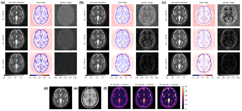
Figure 2: (a-c) Transaxial slice of first noise realization, bias image (mean minus ground truth) and standard deviation image of the 30 simulated noise realizations for CR (a), AGR (b) and AGRdm (c). The level of regularization ($\beta$ / $\beta_{u}$) is increasing by a factor of 3 between rows from top to bottom to show the behaviour of the different reconstructions at different levels of regularization. (d) ground truth sodium image based on brainweb phantom. (e) proton T1 structural prior image used for AGR. The red arrow indicates the added lesion in the sodium ground truth images that is not present in the structural prior image. (f) estimated effective monoexponential $T_{2}^{*}$ time of AGRdm for different $\beta_{u}$

		mean estimated
region	$\beta_{u}$	$T_{2}^{*}$ (ms)
cortial	3e-4	8.6
grey	1e-3	8.4
matter	3e-3	8.3
white	3e-4	6.5
matter	1e-3	5.8
	3e-3	5.7
ventricles	3e-4	24.2
	1e-3	30.8
	3e-3	36.8

Table 2: Mean effective monoexponential $T_{2}^{*}$ times estimated in AGRdm of the simulated brainweb data in different regions of interest for different levels of $\beta_{u}$.

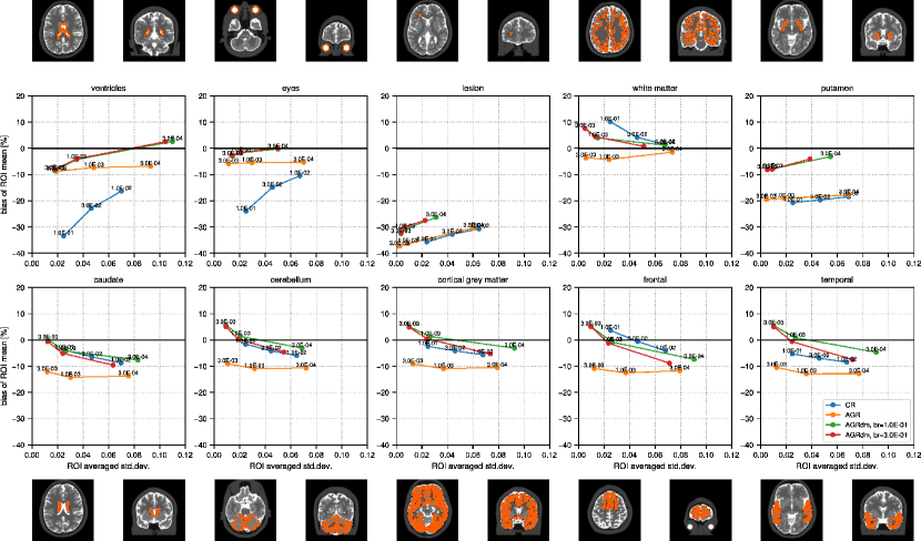
Figure 3: Regional bias noise curves calculated from 30 noise realizations from data simulated based on the brainweb phantom as a function of the regularization weight $\beta_{u}$ shown next to the curves. Every subplot shows the result for a different region of interest (ROI) which are depicted above / below the subplots in a transaxial and coronal slice.

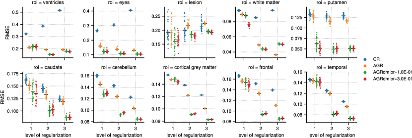
Figure 4: Regional root-mean-square error (RMSE) for all reconstructions and all 30 noise noise realizations (colored dots) for three levels of regularization (1 = low, 2 = medium, 3 = high). The mean regional RMSE across all noise realizations is indicated by black horizontal lines.

4 Results

4.1 Simulation experiments

Figure 2 shows the first noise realization, the bias (mean over all noise realizations minus ground truth) image and the standard deviation image for the conventional reconstruction (CR) using a standard quadratic difference prior, the anatomically-guided reconstruction of the first echo without signal decay modeling (AGR) and the anatomically-guided reconstruction of the data of both echos including signal decay estimation and modeling (AGRdm) for three different levels of image regularization ($\beta_{u}$). The corresponding quantitative regional bias-noise curves as well as illustrations of all ROIs are shown in Fig. 3.

Comparing the image quality of the first noise realization in Fig. 2, it can be seen that at the medium and high level of regularization, the boundaries between GM, WM and CSF are clearly visible in AGR and AGRdm, illustrating the difference in GM and WM sodium concentration which is hardly visible in CR. Moreover, both AGRs show much better separation of CSF contained in sulci between the GM gyri.

In the conventional reconstruction, higher levels of regularization cause loss of resolution, accompanied by more severe partial volume effects (PVE) leading to more negative bias in the ventricles, the eyes and the putamen, which are all structures surrounded by tissues with lower sodium concentration as shown in the top row of Fig. 3. In white matter, which is surrounded by regions with higher sodium concentration, the same effect leads to positive bias. In all those ROIs, AGRdm shows the least amount of bias at a given noise level.

In the cortical gray matter ROIs, shown in the bottom row of Fig. 3, the situation is more complex. In those regions, AGRdm shows has the best bias vs noise trade-off, whilst AGR suffers from consistent negative bias that is bigger than the bias seen in CR. This is because, in cortical gray matter, the positive bias due to spill-over from CSF, the negative bias due to spill-in to white matter and the signal loss due to $T_{2}^{*}$ decay seem to cancel for CR. In AGR without decay modeling, where the spill-over from CSF is strongly reduced, the negative bias of around -10% due to $T_{2}^{*}$ decay becomes noticeable and comparable to the value one would expect given an echo time of 0.455 ms, and short/long $T_{2}^{*}$ times of 3/20 ms.

From the standard deviation images in Fig. 2 it is obvious that the variability in the conventional reconstructions is very homogeneous across the image, whereas the variability in the structure-guided reconstruction is more concentrated around tissue boundaries. The bias images in Fig. 2 and the bias noise plot of the lesion ROI show that in the added sodium white matter lesion, which is not present in the anatomical prior image, the AGRs show negative bias. However, the bias noise trade-off is not inferior compared to the conventional reconstruction.

Figure 4 demonstrates that AGRdm shows the lowest RMSE values across all ROIs except for white matter where AGR has slightly lower RMSE. In all ROIs with correct anatomical prior information, AGR and AGRdm show the lowest RMSE values at the highest level of regularization.

Table 2 shows the effective monoexponential $T_{2}^{*}$ times estimated with AGRdm in different regions of interest. In cortical grey matter and white matter, the estimated effective monoexponential $T_{2}^{*}$ is in between the assigned short and long $T_{2}^{*}$ values used for the biexponential decay simulation (3/20 ms for grey matter, 3/18 ms for white matter). In the ventricles, the estimated $T_{2}^{*}$ times show negative bias with respect to the true monoexponential $T_{2}^{*}$ time for CSF used in the decay simulation (50 ms).

Supporting Table S1 shows the regional bias of AGRdm using the known biexponential decay model compared to AGRdm using the estimated and simplified monoexponential model. Depending on the level of regularization, the bias in cortical grey matter is reduced from -5.4% - 4.9% for AGRdm using the estimated monoexponential model to (0.8% - 2.3%). A similar trend - a bias reduction by a few percentage points - is also seen in the other regions. Moreover, it can be seen that AGR without any decay model suffers from more bias in all regions except white matter at high levels of regularization.

4.2 In vivo experiments

Figures 5, 6, and 7 show the conventional (CR) and anatomically-guided sodium reconstruction without and with signal decay estimation and modeling (AGR and AGRdm) for the three dual echo sodium acquisitions. In all three cases, the boundaries between GM, WM and CSF are much better defined in the anatomically-guided reconstructions, leading, e.g., to a clearer separation between the sodium concentration in GM and WM and also between the CSF in the sulci and cortical gray matter. Moreover, within WM and GM, both AGRs are less noisy compared to the conventional reconstruction. The estimated decay ratio image (the exponential transformation of the effective estimated monoexponential $T_{2}^{*}$ time) clearly shows the relatively slow signal decay in CSF ($r$ close to 1) and faster decay in GM and WM. Figure 8 shows a comparison of the sodium concentration of GM and WM in the cortical region obtained with the three reconstructions in all three cases. The higher cortical GM to WM contrast of AGRdm that can be also clearly seen in Fig. 5 is also confirmed in the plot of cortical GM to WM sodium concentration displayed in the right of Fig. 8. Morever, AGR and AGRdm also lead to higher GM to brainstem sodium concentration ratios which are more in line with the ratios of healthy controls reported in [7] where partial volume correction was applied post reconstruction in image space.

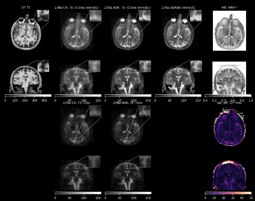
Figure 5: Dual echo sodium reconstructions of a healthy control (60yr, M) acquired on a 3T Siemens Prisma. (top left): ¹H T1 used as anatomical prior. (top 2nd from left): conventional reconstruction (CR) of the first echo (top middle): anatomically-guided reconstruction of the first echo without signal decay modeling (AGR) (top 2nd from right): anatomically-guided reconstruction of both echos including signal decay estimation and modeling (AGRdm). (top right): estimated ratio between the first and second echo ($r$) used for the monoexponential signal decay modeling. (bottom 2nd from left): conventional reconstruction (CR) of the second echo (bottom middle): anatomically-guided reconstruction of the second echo without signal decay modeling (AGR) (bottom right): effective estimated monoexponential $T_{2}^{*}$ time calculated from $r$. The signal intensity of all sodium images (including the 2nd echo images of CR and AGR) is normalized to the mean signal intensity of AGRdm in vitreous humor (145 mmol/L) and shown using the same color scale. Due to the impact of the $T_{2}^{*}$ decay, the units of the second echo images are not labeled as mmol/L.

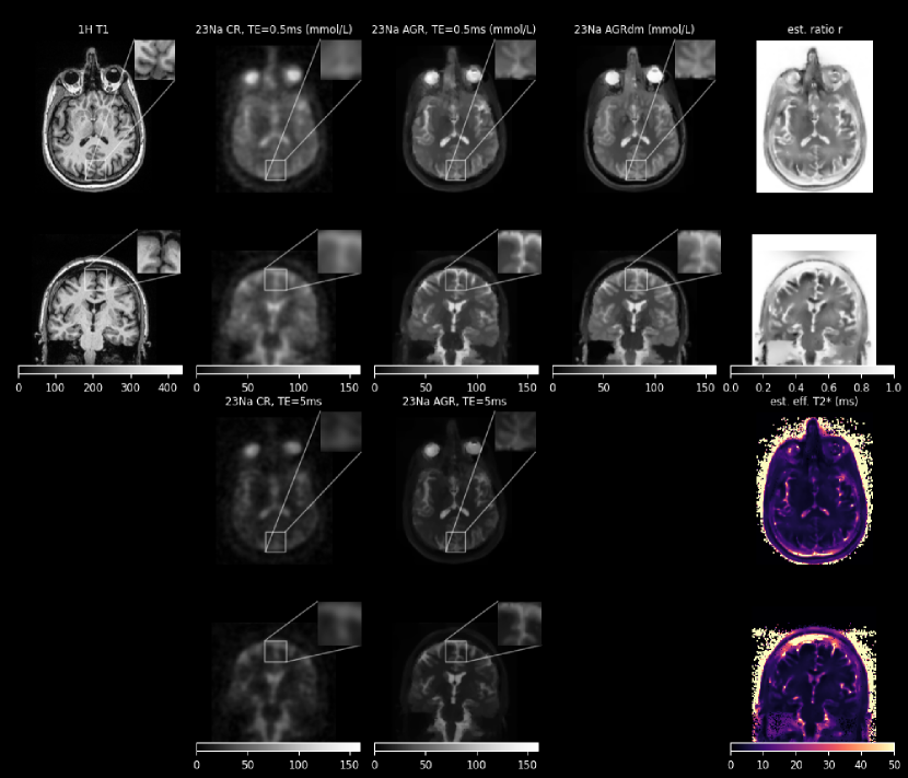
Figure 6: Same as Fig. 5 for the second healthy control (65yr, F).

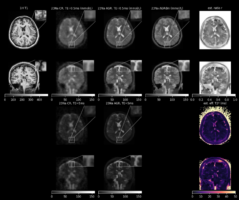
Figure 7: Same as Fig. 5 for the second healthy control (42yr, F).

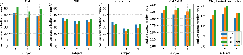
Figure 8: Regional quantification of TSC in GM and WM (left and middle) and the TSC GM/WM ratio (right) in three healthy controls for all different sodium reconstruction algorithms.

5 Discussion

In this work, we have presented a framework for joint reconstruction and transverse signal decay estimation and modeling of dual echo ²³Na using anatomical guidance. Compared to the existing works of Zhao et al. [25] and Gnahm et al. [24], our method has the advantages that (i) no segmentation of the prior image is needed, (ii) a better segmentation-free anatomical prior (dTV) is used and (iii) that the local $T_{2}^{*}$ signal decay can be estimated and modeled during reconstruction. The latter is important since rapid spatially-varying transverse signal decay, e.g. at tissue-air interfaces, leads to local widening of the point-spread function (PSF), which complicates image deblurring and also leads to spatially-varying signal loss in the first echo image acquired at a finite time after excitation (e.g. 0.455 ms). As already mentioned in [24, 25] anatomically-guided ²³Na reconstruction could have a major impact on clinical sodium MR imaging at 3T, since it allows to reconstruct high SNR images with a high level of detail even at 3T enabling improved ²³Na imaging at standard field strengths. Note that although this work focuses on sodium data acquired on 3T systems, application of our framework to data acquired at higher field strengths is straightforward.

A current drawback of our framework is the relatively long reconstruction time. Using a state-of-the-art GPU, a joint reconstruction using 2000 overall updates in Alg. 1 takes roughly 1h. However, it is to be expected that these reconstruction times can be significantly shortened by using stochastic optimization algorithms to solve (15), e.g., the stochastic version PDHG [34] and stochastic gradient descent and by using more efficient implementations of the NUFFT.

Another limitation of our framework is the fact that most anatomically-guided priors (including dTV) are based on the assumption that edges in the prior image and in the image to be reconstructed are present at the same locations. As shown in several works, exploiting this prior knowledge during reconstruction can be very beneficial for joint denoising and debluring. However, all images reconstructed with anatomical prior knowledge must be interpreted with caution if the assumption behind the anatomical prior is violated. This potentially means that small structures that are not present in the structural prior image could be lost (smoothed away) when using high levels of regularization and, therefore, the reconstruction framework must be carefully tuned to avoid such effects. Note, however, that Fig. 4 demonstrated that the bias versus noise trade-off of AGR and AGRdm in the sodium lesion absent in the structural prior image was not inferior to CR. This can be understood by taking into account that dTV reduces to "normal" TV if no structural prior information is available (locally flat prior image).

In this work, the structural prior proton MPRAGE was acquired with a different coil yielding superior proton image quality compared to the dual-tuned coil. A requirement of our current implementation is that the proton MPRAGE had to be rigidly registered to the sodium CR because of patient repositioning, before running AGR and AGRdm. According to our experience the rigid registration of the proton MPRAGE to the sodium CR is stable and accurate. However, small residual mis-alignments cannot be fully excluded, and, threfore, registration of the proton MPRAGE and the sodium CR should be always verified before running AGR or AGRdm since structural priors require accurate alignment of the structural prior image.

The bias vs. noise analysis of the simulated data has shown that AGRdm shows less bias compared AGR and CR. This reduction of partial volume effects, especially in the ventricles, white matter, and gray matter, should help to improve quantification of tissue sodium concentration in clinical acquisitions. The comparison of AGRdm with estimated monoexponential and AGRdm with known biexponential decay model, which is in not availalbe in practice, showed that using the estimated and simplified monoexponential model only leads to a slight increase of a few percentage points in the regional bias. Taking into account that not modeling the decay in AGR leads to much stronger bias, especially in grey matter, we are confident that estimating and using a simplified monoexponential model during AGR leads to an overall reduction of the regional bias in tissue sodium quantification.

Since no ground truth for the local sodium concentration in the in vivo experiments was available, we decided to quantify the gray matter to brainstem ratio as proposed by Haeger et al.[7] in the analysis of 3T sodium images corrected for partial volume effects after reconstruction of 52 patients with Alzheimer’s disease and 34 controls. Compared to the ratios calculated in the conventional reconstruction (CR), the ratios obtained from AGR and AGRdm in the three control cases of our work were closer to the range reported for controls by Haeger et al. (1.6 - 2.0). Partial volume correction post reconstruction is another option to reduce PVEs. Note, however, that the PV-corrected sodium image shown in Fig. 1 of [7] shows much less anatomical detail compared to the AGR or AGRdm images shown in this work. A more detailed investigation of the impact of anatomically guided reconstruction on regional sodium concentration quantification in different ROIs in a larger patient cohort is beyond the scope of the work and left for future research. Note that the three human dual echo sodium data sets used in this work were acquired for a different research project and used retrospectively. For prospective acquisitions, it is recommended to use more averages for the acquisition of the second echo since it suffers from lower SNR due to signal decay.

Finally, further gains in quantification accuracy can be gained through the use of the proposed approach by incorporating the use of $B_{1}$ field mapping (to correct for RF coil "shading") and $B_{0}$ inhomogeneity k-space distortion correction. As shown in [35], the former can be efficiently carried out through time-efficient $B_{1}$ mapping via the phase-sensitive [36] Bloch-Siegert shift [37] or the double-angle method [38]. The later correction, on the other hand, could be performed very efficiently using a linearized version of the $B_{0}$ inhomogeneity map [39] as these effects are typically much smaller than in conventional proton MRI due to sodium’s lower gyromagnetic ratio.

6 Conclusion

Our proposed framework for resolution enhancement, noise suppression, and joint T2* decay estimation using dual-echo sodium-23 MR data and anatomically-guided reconstruction is capable of producing high SNR sodium images with high levels of anatomical detail at 3T, reducing the negative impact of partial volume effects on regional quantification in ²³Na MR images.

Financial disclosure

None reported.

Conflict of interest

The authors declare no potential conflict of interests.

Supporting information

The following supporting information is available as part of the online article: support_material.pdf containing supporting Table S1.

Data Availability Statement

The input data that support the findings of the simulation study are openly available in the BrainWeb database at https://brainweb.bic.mni.mcgill.ca/brainweb/anatomic_normal_20.html. The input data of the in vivo experiments are not shared. The source code used to generate the results of this manuscript is available at https://github.com/gschramm/sodium_mr_agr_paper.

References

- [1] Ronald Ouwerkerk et al. “Tissue Sodium Concentration in Human Brain Tumors as Measured with 23Na MR Imaging” Publisher: Radiological Society of North America In Radiology 227.2, 2003, pp. 529–537 DOI: 10.1148/radiol.2272020483
- [2] R. Bartha, J.. Megyesi and C.. Watling “Low-grade glioma: correlation of short echo time 1H-MR spectroscopy with 23Na MR imaging” In AJNR. American journal of neuroradiology 29.3, 2008, pp. 464–470 DOI: 10.3174/ajnr.A0854
- [3] Muhammad S. Hussain et al. “Sodium imaging intensity increases with time after human ischemic stroke” In Annals of Neurology 66.1, 2009, pp. 55–62 DOI: https://doi.org/10.1002/ana.21648
- [4] FE Boada et al. “Sodium MRI and the Assessment of Irreversible Tissue Damage During Hyper-Acute Stroke” In Transl. Stroke Res. 3, 2012
- [5] E.A. Mellon et al. “Sodium MR Imaging Detection of Mild Alzheimer Disease: Preliminary Study” In American Journal of Neuroradiology 30.5, 2009, pp. 978–984 DOI: 10.3174/ajnr.A1495
- [6] SA Mohamed et al. “Evaluation of Sodium (23Na) MR-imaging as a Biomarker and Predictor for Neurodegenerative Changes in Patients With Alzheimer’s Disease” In In Vivo 35.1 International Institute of Anticancer Research, 2021, pp. 429–435 DOI: 10.21873/invivo.12275
- [7] Alexa Haeger et al. “3T sodium MR imaging in Alzheimer’s disease shows stage-dependent sodium increase influenced by age and local brain volume” In NeuroImage: Clinical 36, 2022, pp. 103274 DOI: https://doi.org/10.1016/j.nicl.2022.103274
- [8] Guillaume Madelin and Ravinder R. Regatte “Biomedical applications of sodium MRI in vivo” In Journal of Magnetic Resonance Imaging 38.3, 2013, pp. 511–529 DOI: https://doi.org/10.1002/jmri.24168
- [9] N. Shah, Wieland A. Worthoff and Karl-Josef Langen “Imaging of sodium in the brain: a brief review” In NMR in Biomedicine 29.2, 2016, pp. 162–174 DOI: 10.1002/nbm.3389
- [10] Keith R. Thulborn “Quantitative sodium MR imaging: A review of its evolving role in medicine” In NeuroImage 168, Neuroimaging with Ultra-high Field MRI: Present and Future, 2018, pp. 250–268 DOI: 10.1016/j.neuroimage.2016.11.056
- [11] A. Hagiwara et al. “Sodium MR Neuroimaging” In AJNR. American journal of neuroradiology 42.11, 2021, pp. 1920–1926 DOI: 10.3174/ajnr.A7261
- [12] Robert W. Stobbe and Christian Beaulieu “Calculating potential error in sodium MRI with respect to the analysis of small objects” In Magnetic Resonance in Medicine 79.6, 2018, pp. 2968–2977 DOI: https://doi.org/10.1002/mrm.26962
- [13] J.A. Fessler, N.H. Clinthorne and W.L. Rogers “Regularized emission image reconstruction using imperfect side information” Conference Name: IEEE Transactions on Nuclear Science In IEEE Transactions on Nuclear Science 39.5, 1992, pp. 1464–1471 DOI: 10.1109/23.173225
- [14] B Lipinski et al. “Expectation maximization reconstruction of positron emission tomography images using anatomical magnetic resonance information” In IEEE Transactions on Medical Imaging 16.2, 1997, pp. 129–136 DOI: 10.1109/42.563658
- [15] Kristof Baete et al. “Anatomical-based FDG-PET reconstruction for the detection of hypo-metabolic regions in epilepsy” ISBN: 0278-0062 In IEEE Transactions on Medical Imaging 23.4, 2004, pp. 510–519 DOI: 10.1109/TMI.2004.825623
- [16] JE Bowsher and Hong Yuan “Utilizing MRI information to estimate F18-FDG distributions in rat flank tumors” In Nuclear Science Symposium Conference Record, 2004 IEEE 4.C, 2004, pp. 2488–2492 DOI: 10.1109/NSSMIC.2004.1462760
- [17] Kathleen Vunckx et al. “Evaluation of three MRI-based anatomical priors for quantitative PET brain imaging” In IEEE Transactions on Medical Imaging 31.3, 2012, pp. 599–612 DOI: 10.1109/TMI.2011.2173766
- [18] Florian Knoll et al. “Joint MR-PET reconstruction using a multi-channel image regularizer” In IEEE Transactions on Medical Imaging 36.1, 2016, pp. 1–16 DOI: 10.1109/TMI.2016.2564989
- [19] Matthias Ehrhardt et al. “PET Reconstruction with an Anatomical MRI Prior using Parallel Level Sets” In IEEE Transactions on Medical Imaging 35.9, 2016, pp. 2189–2199 DOI: 10.1109/TMI.2016.2549601
- [20] Georg Schramm et al. “Evaluation of Parallel Level Sets and Bowsher’s Method as Segmentation-Free Anatomical Priors for Time-of-Flight PET Reconstruction” In IEEE Transactions on Medical Imaging 37.2, 2017, pp. 590–603 DOI: 10.1109/TMI.2017.2767940
- [21] Z.-P. Liang and P.C. Lauterbur “A generalized series approach to MR spectroscopic imaging” In IEEE Transactions on Medical Imaging 10.2, 1991, pp. 132–137 DOI: 10.1109/42.79470
- [22] Justin P. Haldar, Diego Hernando, Sheng-Kwei Song and Zhi-Pei Liang “Anatomically constrained reconstruction from noisy data” In Magnetic Resonance in Medicine 59.4, 2008, pp. 810–818 DOI: 10.1002/mrm.21536
- [23] Matthias J. Ehrhardt and Marta M. Betcke “Multicontrast MRI Reconstruction with Structure-Guided Total Variation” In SIAM Journal on Imaging Sciences 9.3, 2016, pp. 1084–1106 DOI: 10.1137/15M1047325
- [24] Christine Gnahm and Armin M. Nagel “Anatomically weighted second-order total variation reconstruction of 23Na MRI using prior information from 1H MRI” In NeuroImage 105, 2015, pp. 452–461 DOI: 10.1016/j.neuroimage.2014.11.006
- [25] Yibo Zhao et al. “High-resolution sodium imaging using anatomical and sparsity constraints for denoising and recovery of novel features” In Magnetic Resonance in Medicine 86.2, 2021, pp. 625–636 DOI: 10.1002/mrm.28767
- [26] Matthias J. Ehrhardt, Ferdia A. Gallagher, Mary A. McLean and Carola-Bibiane Schönlieb “Enhancing the spatial resolution of hyperpolarized carbon-13 MRI of human brain metabolism using structure guidance” In Magnetic Resonance in Medicine 87.3, 2022, pp. 1301–1312 DOI: https://doi.org/10.1002/mrm.29045
- [27] J.A. Fessler and B.P. Sutton “Nonuniform fast Fourier transforms using min-max interpolation” In IEEE Transactions on Signal Processing 51.2, 2003, pp. 560–574 DOI: 10.1109/TSP.2002.807005
- [28] D.C. Noll et al. “A homogeneity correction method for magnetic resonance imaging with time-varying gradients” In IEEE Transactions on Medical Imaging 10.4, 1991, pp. 629–637 DOI: 10.1109/42.108599
- [29] Douglas C. Noll et al. “Deblurring for non-2D fourier transform magnetic resonance imaging” In Magnetic Resonance in Medicine 25.2, 1992, pp. 319–333 DOI: https://doi.org/10.1002/mrm.1910250210
- [30] Matthias J. Ehrhardt “Multi-modality Imaging with Structure-Promoting Regularizers” In Handbook of Mathematical Models and Algorithms in Computer Vision and Imaging: Mathematical Imaging and Vision Cham: Springer International Publishing, 2021, pp. 1–38 DOI: 10.1007/978-3-030-03009-4_58-1
- [31] D.L. Collins et al. “Design and construction of a realistic digital brain phantom” In IEEE Transactions on Medical Imaging 17.3, 1998, pp. 463–468 DOI: 10.1109/42.712135
- [32] Fernando E. Boada et al. “Fast three dimensional sodium imaging” In Magnetic Resonance in Medicine 37.5, 1997, pp. 706–715 DOI: https://doi.org/10.1002/mrm.1910370512
- [33] A. Chambolle and T. Pock “A First-Order Primal-Dual Algorithm for Convex Problems with Applications to Imaging” In Journal of Mathematical Imaging and Vision 40, 2011, pp. 120–145 DOI: 10.1007/s10851-010-0251-1
- [34] Antonin Chambolle, Matthias J. Ehrhardt, Peter Richtarik and Carola Bibiane Schonlieb “Stochastic primal-dual hybrid gradient algorithm with arbitrary sampling and imaging applications” In SIAM Journal on Optimization 28.4, 2018, pp. 2783–2808 DOI: 10.1137/17M1134834
- [35] Jonathan Lommen, Simon Konstandin, Philipp Krämer and Lothar R. Schad “Enhancing the quantification of tissue sodium content by MRI: time-efficient sodium B1 mapping at clinical field strengths” In NMR in Biomedicine 29.2, 2016, pp. 129–136 DOI: 10.1002/nbm.3292
- [36] Glen R. Morrell “A phase-sensitive method of flip angle mapping” In Magnetic Resonance in Medicine 60.4, 2008, pp. 889–894 DOI: 10.1002/mrm.21729
- [37] Laura I. Sacolick, Florian Wiesinger, Ileana Hancu and Mika W. Vogel “B1 mapping by Bloch-Siegert shift” In Magnetic Resonance in Medicine 63.5, 2010, pp. 1315–1322 DOI: 10.1002/mrm.22357
- [38] E.. Insko and L. Bolinger “Mapping of the Radiofrequency Field” In Journal of Magnetic Resonance, Series A 103.1, 1993, pp. 82–85 DOI: https://doi.org/10.1006/jmra.1993.1133
- [39] Pablo Irarrazabal, Craig H. Meyer, Dwight G. Nishimura and Albert Macovski “Inhomogeneity correction using an estimated linear field map” In Magnetic Resonance in Medicine 35.2, 1996, pp. 278–282 DOI: https://doi.org/10.1002/mrm.1910350221