Tensor Golub Kahan based on Einstein product

Abstract

The Singular Value Decomposition (SVD) of matrices is a widely used tool in scientific computing. In many applications of machine learning, data analysis, signal and image processing, the large datasets are structured into tensors, for which generalisations of SVD have already been introduced, for various types of tensor-tensor products. In this article, we present innovative methods for approximating this generalisation of SVD to tensors in the framework of the Einstein tensor product. These singular elements are called singular values and singular tensors respectively. The proposed method uses the tensor Lanczos bidiagonalization applied to the Einstein product. In most applications, as in the matrix case, the extremal singular values are of special interest. To enhance the approximation of the largest or the smallest singular triplets (singular values and left and right singular tensors), a restarted method based on Ritz augmentation is proposed. Numerical results are proposed to illustrate the effectiveness of the presented method. In addition, applications to video compression and facial recognition are presented.

1 introduction

One of the ubiquitous and challenging problems in mathematics is the extraction of the most relevant information out of large datasets, especially in the domains of data mining, machine learning and deep learning. In the context where data is represented by matrices, the determination of the main features is closely related to the Singular Value Decomposition (SVD) of some matrix, like the covariance matrix for Principal Component Analysis (PCA). More precisely, the main features of the data are related to the largest singular values of a matrix and their associated left and right singular vectors, summarised under the name of singular triplets. Due the generally large size of the datasets, the computation of the SVD is sometimes unrealistic in terms of computational time. This problem has already been addressed in the matrix case by Golub and al. in [18], based on a Lanczos bidiagonalization (LB) algorithm. This approach, which was later refined by Baglama and Reichel in [4], aims to avoid the computation of the SVD of a potentially very large matrix, approximating just a chosen number of the largest (or smallest) singular triplets.

In numerous real world applications, due to the large quantity of information and variables, datasets are often structured as multidimensional arrays, the so-called tensors. A tensor is a multidimensional array of numbers, and can be seen as a generalisation of matrices and vectors. An $N$-order tensor (or $N$-mode tensor) is a $N$ dimensional array (a vector for $N=1$ and a matrix for $N=2$). Various tensor-tensor products have been defined, generalising the matrix-matrix product, as the t-product, and the c-product that have been introduced by Kilmer et all. [20, 11] and the most notorious Einstein product [14]. The t and c-products are defined via matrix-matrix products in the Fourier and Cosine domain, after a Fast Fourier transform (FFT) or Discrete Cosine transform (DCT). These products were first designed only for third-order tensors, although Martin et al. and Bentbib and al. have generalised them for higher order tensor in [21, 16]. Note that in their article [16], the authors also gave a more general tensor-tensor product using any invertible linear transform, the $\mathcal{L}$-product.

In the recent years, tensor-based numerical methods have received a great deal of attention for their ability to address very topical problems. Amongst many other applications, completion problems, which consist of approximating some missing information in large datasets (recommendation systems for customer, restoration of damaged images etc.), see [7, 10] for more details. We can also mention the Tensor Robust Principal Component Analysis (RPCA), which objective is to remove the noise from corrupted data [8], image restoration [6, 9] and numerical meshless methods for the resolution of 3-d PDE’s via Radial Basis Functions (RBF) [15].

The generalisation of the SVD for tensors has been introduced in various ways, depending on the chosen tensor-tensor product. The t-svd, c-svd, and $\mathcal{L}$-svd in [20, 1, 10] are defined via the t-product, the c-product and the $\mathcal{L}$-product, respectively, and have been originally designed for 3-mode tensors. In this paper, we will focus on the SVD associated to the more general Einstein product [12, 13].

The approximation of the largest singular triplets for tensors was first introduced in [19] for 3-mode tensors, using the c-product. This approach was an adaptation to tensors of the matrix Lanczos bidiagonalization. In order to improve the accuracy of this approximation, in [16], the authors generalized the work done by Baglama and Reichel [4] under the t-product, by restarted strategies using Ritz and Harmonic Ritz tensors. This approach gave very satisfactory results in terms of accuracy and were illustrated by applications to facial recognition, image classification and data compression [16, 19].

This paper is outlined as follows: In Section 2, a reminder of the Einstein product and some properties are presented, Section 3 is devoted to the approximation of the tensor singular triplets can by using the tensor Lanczos bidiagonalization associated with the Einstein product, along with a restart strategy by Ritz tensors. Section 4 presents a new Einstein product based PCA technique, and some numerical experiments are presented in Section 5.

2 Definitions and notations

In this section, we review some notations, definitions, and properties linked with tensors. The notations used throughout this paper are the same as those employed by Kolda and Bader in [5]. A real $N$th-order tensor $\mathcal{A}$ is an $N$-dimensional array of real numbers and we denote $\mathbb{R}^{I_{1}\times\ldots\times I_{N}}$ the real vector space of $N$th-order real tensors. The $(i_{1},\ldots,i_{N})^{\text{th}}$ entry of the tensor $\mathcal{A}$ is denoted by $\mathcal{A}_{i_{1}\ldots i_{N}}$. General definitions about foldings, unfoldings, fibers and slices can be found in [5].

First, we describe the n-mode product which defines a multiplication of a tensor by a matrix or a vector.

Definition 1.

[5] Let $\mathcal{A}\in\mathbb{R}^{I_{1}\times\ldots\times I_{N}}$ and $U\in\mathbb{R}^{J\times I_{n}}$ be an $N$-order tensor and a matrix, respectively. The n-mode product between $\mathcal{A}$ and $U$ produces a tensor of size $I_{1}\times\ldots\times I_{n-1}\times J\times I_{n+1}\times\ldots\times I_{N}$, which entries are given by

$$\left(\mathcal{A}\times_{n}U\right)_{i_{1}\ldots i_{n-1}ji_{n+1}\ldots i_{N}}=\sum_{i_{n}=1}^{I_{n}}\mathcal{A}_{i_{1}\ldots i_{N}}U_{ji_{n}}.$$

We recall the following identities :

For all tensor $\mathcal{A}\in\mathbb{R}^{I_{1}\times\ldots\times I_{N}}$ and for all matrices $U\in\mathbb{R}^{J\times I_{n}}$ and $V\in\mathbb{R}^{K\times I_{m}}$, we have

$$\mathcal{A}\times_{n}U\times_{m}V=\mathcal{A}\times_{m}V\times_{n}U.$$

Moreover, if $U\in\mathbb{R}^{J\times I_{n}}$ and $V\in\mathbb{R}^{I_{n}\times J}$, then, we have

$$\mathcal{A}\times_{n}U\times V=\mathcal{A}\times_{n}\left(VU\right).$$

We now give the definition of the n-mode matricization of a tensor.

Definition 2.

[5] Let $\mathcal{A}\in\mathbb{R}^{I_{1}\times\ldots\times I_{N}}$ be an $N$-order tensor. The n-mode matricization of $\mathcal{A}$ is denoted by $\mathcal{A}_{(n)}$ belongs to $\mathbb{R}^{I_{n}\times\prod_{i=1}^{N}I_{i}}$. It maps the $(i_{1},\ldots,i_{N})$-th element fo $\mathcal{A}$ to the $(i_{n},j)$-th element of $\mathcal{A}_{(n)}$ one, such that

$$j=1+\sum_{k=1,k\neq n}^{N}(i_{k}-1)J_{k},\quad\text{with}\quad J_{k}=\prod_{m=1,m\neq m}^{k-1}I_{m}.$$

The following identity gives an interpretation of the n-mode product in terms of a matrix product:

Let $\mathcal{A}\in\mathbb{R}^{I_{1}\times\ldots\times I_{N}}$ and $B\in\mathbb{R}^{J\times I_{n}}$, then we have

$$\mathcal{C}=\mathcal{A}\times_{n}B\Longleftrightarrow\mathcal{C}_{(n)}=B\mathcal{A}_{(n)},$$ (1)

where $\mathcal{C}_{(n)}$ and $\mathcal{A}_{(n)}$ are respectively the n-mode matricization of $\mathcal{A}$ and $\mathcal{C}$.

Next, we recall the Einstein product [14, 12, 13].

Definition 3.

[12] Let $\mathcal{A}\in\mathbb{R}^{I_{1}\times\ldots\times I_{L}\times K_{1}\times\dots\times K_{N}}$ and $\mathcal{B}\in\mathbb{R}^{K_{1}\times\ldots\times K_{N}\times J_{1}\times\ldots\times J_{N}}$. The Einstein product between $\mathcal{A}$ and $\mathcal{B}$ is the tensor of size $I_{1}\times\ldots\times I_{L}\times J_{1}\times\ldots\times J_{N}$ whose elements are defined by

$$\left(\mathcal{A}*_{N}\mathcal{B}\right)_{i_{1}\ldots i_{L}j_{1}\ldots j_{M}}=\sum_{k_{1},\ldots,k_{N}=1}^{K_{1},\ldots,K_{N}}\mathcal{A}_{i_{1}\ldots i_{L}k_{1}\ldots k_{N}}\mathcal{B}_{k_{1}\ldots k_{N}j_{1}\ldots j_{M}}.$$

The following definitions will be needed in the sequel.

Definition 4.

• Transpose tensor: For a given tensor $\mathcal{A}\in\mathbb{R}^{I_{1}\times\ldots\times I_{N}\times J_{1}\times\ldots\times J_{M}}$ the transpose tensor $\mathcal{B}$ of $\mathcal{A}$ denoted by $\mathcal{A}^{T}$ is the tensor of size $J_{1}\times\ldots\times J_{M}\times I_{1}\times\ldots\times I_{N}$ whose elements are $\mathcal{B}_{j_{1}\dots j_{M}i_{1}\dots i_{N}}=\mathcal{A}_{i_{1}\dots i_{N}j_{1}\dots j_{M}}$.

• Diagonal tensor: A tensor $\mathcal{D}\in\mathbb{R}^{I_{1}\times\ldots\times I_{N}\times J_{1}\times\ldots\times J_{M}}$ is a diagonal tensor if
  $\mathcal{D}_{i_{1}\dots i_{N}j_{1}\dots j_{M}}=0$ for all $i_{k}\neq j_{k}$ with $k\in\{1,\ldots,\min(N,M)\}$.

• Identity tensor: $\mathcal{I}_{N}\in\mathbb{R}^{I_{1}\times\ldots\times I_{N}\times I_{1}\times\ldots\times I_{N}}$ is called an identity tensor if it is diagonal and all its diagonal entries are ones.

• Invertible tensor: A tensor $\mathcal{A}\in\mathbb{R}^{I_{1}\times\ldots I_{N}\times I_{1}\times\ldots\times I_{N}}$ is invertible if and only if there exists a tensor $\mathcal{X}\in\mathbb{R}^{I_{1}\times\ldots I_{N}\times I_{1}\times\ldots\times I_{N}}$ such that

  $$\mathcal{A}*_{N}\mathcal{X}=\mathcal{X}*_{N}\mathcal{A}=\mathcal{I}_{N}.$$

  If such a tensor exists, it is unique. It is called the inverse of $\mathcal{A}$ and is denoted by $\mathcal{A}^{-1}$.

Let $\mathcal{A},\mathcal{B}$ two tensors in $\mathbb{R}^{I_{1}\times\ldots\times I_{N}\times J_{1}\times\ldots\times J_{M}}$. The inner product between $\mathcal{A}$ and $\mathcal{B}$ is defined by

$$\langle\mathcal{A},\mathcal{B}\rangle={\tt tr}\left(\mathcal{A}^{T}*_{N}\mathcal{B}\right),$$

where, the trace of $\mathcal{A}\in\mathbb{R}^{I_{1}\times\ldots\times I_{N}\times I_{1}\times\ldots\times I_{N}}$ is defined as

$${\tt tr}\left(\mathcal{A}\right)=\sum_{i_{1},\ldots,i_{N}=1}^{I_{1},\ldots,I_{N}}\mathcal{A}_{i_{1}\ldots i_{N}i_{1}\dots i_{N}}.$$

If we have $\langle\mathcal{A},\mathcal{B}\rangle=0$, then we say that $\mathcal{A}$ and $\mathcal{B}$ are orthogonal.
The corresponding norm is the tensor Frobenius norm given by

$$\left\|\mathcal{A}\right\|_{F}=\sqrt{{\tt tr}\left(\mathcal{A}^{T}*_{N}\mathcal{A}\right)}.$$

Proposition 5.

[13] Let $\mathcal{A}\in\mathbb{R}^{I_{1}\times\ldots\times I_{L}\times K_{1}\times\ldots\times K_{N}}$ and $\mathcal{B}\in\mathbb{R}^{K_{1}\times\ldots\times K_{N}\times J_{1}\times\ldots\times J_{M}}$. Then

$$\left(\mathcal{A}*_{N}\mathcal{B}\right)^{T}=\mathcal{B}^{T}*_{N}\mathcal{A}^{T}.$$

In the sequel, for all considered tensor $\mathcal{A}\in\mathbb{R}^{I_{1}\times\ldots\times I_{N}\times J_{1}\times\ldots\times J_{M}}$, we will suppose that $M\leq N$.

The generalization of the svd under the Einstein product is defined as follows :

Theorem 6.

[13] Let us consider a tensor $\mathcal{A}\in\mathbb{R}^{I_{1}\times\ldots\times I_{N}\times J_{1}\times\ldots\times J_{M}}$. The singular value decomposition (SVD) of $\mathcal{A}$ is given by a decomposition

$$\mathcal{A}=\mathcal{U}*_{N}\mathcal{S}*_{M}\mathcal{V}^{T},$$

where $\mathcal{U}\in\mathbb{R}^{I_{1}\times\ldots\times I_{N}\times I_{1}\times\ldots\times I_{N}}$, $\mathcal{V}\in\mathbb{R}^{J_{1}\times\ldots\times J_{M}\times J_{1}\times\ldots\times J_{M}}$, and $\mathcal{S}\in\mathbb{R}^{I_{1}\times\ldots\times I_{N}\times J_{1}\times\ldots\times J_{M}}$ is a diagonal tensor satisfying:

• If $M=N$

  $$\mathcal{S}_{i_{1}\ldots i_{N}j_{1}\ldots j_{N}}=\left\{\begin{array}[]{ll}\mu_{i_{1}\ldots i_{N}}\text{\leavevmode\nobreak\ if\leavevmode\nobreak\ \leavevmode\nobreak\ }(i_{1},\ldots,i_{N})=(j_{1},\ldots,j_{N}),\\ 0\text{\leavevmode\nobreak\ if\leavevmode\nobreak\ \leavevmode\nobreak\ }(i_{1},\ldots,i_{N})\neq(j_{1},\ldots,j_{N}).\end{array}\right.$$

• If $M<N$

  $$\mathcal{S}_{i_{1}\ldots i_{N}j_{1}\ldots j_{M}}=\left\{\begin{array}[]{ll}\mu_{i_{1}\ldots i_{M}}\text{\leavevmode\nobreak\ if\leavevmode\nobreak\ \leavevmode\nobreak\ }(i_{1},\ldots,i_{M})=(j_{1},\ldots,j_{M}),\;(i_{M+1},\ldots,i_{N})=(1,\ldots,1),\\ 0\quad\text{otherwise}.\end{array}\right.$$

where the positive real numbers $\mu_{i_{1}\ldots i_{M}}$ are called the singular values of $\mathcal{A}$.

Assume that we have $\mathcal{A}\in\mathbb{R}^{I_{1}\times\ldots\times I_{N}\times J_{1}\times\ldots\times J_{M}}$ and let $\widetilde{I}_{i}=\min(I_{i},J_{i})$ for $i=1,\ldots,M$. Let us consider the tensor svd given in the above theorem. Therefore, we can write :

$$\mathcal{A}=\sum_{i_{1},\ldots,i_{M}=1}^{\widetilde{I}_{1},\ldots,\widetilde{I}_{M}}\mu_{i_{1}\ldots i_{M}}\mathcal{U}_{i_{1}\ldots i_{M}}*_{M}\left(\mathcal{V}_{i_{1}\ldots i_{M}}\right)^{T},$$

where $\mathcal{U}_{i_{1}\ldots i_{M}}\in\mathbb{R}^{I_{1}\times\ldots\times I_{N}}$ and $\mathcal{V}_{i_{1}\ldots i_{M}}\in\mathbb{R}^{J_{1}\times\ldots\times J_{N}}$ are called the left and the right singular tensors respectively. Note that we have :

• If $M=N$, $\mathcal{U}_{i_{1}\ldots i_{M}}=\mathcal{U}(:,\ldots,:,i_{1},\ldots,i_{M})$,

• If $M<N$, $\mathcal{U}_{i_{1}\ldots i_{M}}=\mathcal{U}(:,\ldots,:,i_{1},\ldots,i_{M},1,\ldots,1)$,

• $\mathcal{V}_{i_{1}\ldots i_{M}}=\mathcal{V}(:,\ldots,:,i_{1},\ldots,i_{M})$.

The singular values $\mu_{i_{1}\ldots I_{N}}$ are ordered decreasingly, i.e.,

$$\mu_{1,1,\ldots,1}\geq\mu_{2,1,\ldots,1}\geq\dots\geq\mu_{\widetilde{I}_{1},1,\ldots,1}\geq\ldots\geq\mu_{\widetilde{I}_{1},\widetilde{I}_{2},\ldots,\widetilde{I}_{N}}.$$

Notice that $\mathcal{A}$ admits $\widetilde{I}_{1}\widetilde{I}_{2}\ldots\widetilde{I}_{N}$ singular values and left and right singular tensors.
In the sequel, for $k\in\mathbb{N}^{*}$, $s_{k}$, $\mathcal{U}_{k}$ and $\mathcal{V}_{k}$ will denote the $k^{th}$ singular value and the left and right singular tensors respectively and $\left\{s_{k},\mathcal{U}_{k},\mathcal{V}_{k}\right\}$ will be called the $k^{th}$ singular triplet of $\mathcal{A}$.

3 The large tensor svd based on tensor Krylov subspace

The tensors involved in many problems are large, making the computation of the SVD computationally very challenging. Nevertheless, in almost all applications, only the largest singular triplets are required. The well-known Golub-Kahan method has been used to address this issue in the matrix case and very useful refinements have been proposed by Reichel and Baglama [4]. More recently, in [16, 19], the authors proposed a generalization of those refinements to the t/c or $L$-products for 3th-order tensors, with applications to PCA, image recognition and classification problems. In this section, we propose an approximation method of singular triplets of large tensors under the Einstein product which is based on the tensor Lanczos bidiagonalization.

3.1 Einstein tensor Lanczos bidiagonalization

Let $\mathcal{A}\in\mathbb{R}^{I_{1}\times\ldots\times I_{N}\times J_{1}\times\ldots\times J_{M}}$ be a large tensor, $\mathcal{P}\in\mathbb{R}^{J_{1}\times\ldots\times J_{N}}$ and $m\in\mathbb{N}^{*}$such as $m\leq\min(I_{1}\ldots I_{N},J_{1}\ldots J_{M})$. An $m$ tensor Lanczos diagonalization (Golub Kahan) process consists in constructing two orthogonal subspaces from the following Krylov subspaces

$$\textbf{K}_{m}\left(\mathcal{A}^{T}*_{N}\mathcal{A},\mathcal{P}\right)={\tt span}\left\{\mathcal{P},\left(\mathcal{A}^{T}*_{N}\mathcal{A}\right)*_{M}\mathcal{P},\ldots,\left(\mathcal{A}^{T}*_{N}\mathcal{A}\right)^{m-1}*_{M}\mathcal{P}\right\},$$

$$\textbf{K}_{m}\left(\mathcal{A}*_{M}\mathcal{A}^{T},\mathcal{Q}\right)={\tt span}\left\{\mathcal{Q},\left(\mathcal{A}*_{M}\mathcal{A}^{T}\right)*_{N}\mathcal{Q},\ldots,\left(\mathcal{A}*_{M}\mathcal{A}^{T}\right)^{m-1}*_{N}\mathcal{Q}\right\},$$

with $\left\|\mathcal{P}\right\|_{F}=1$, and $\mathcal{Q}=\mathcal{A}*_{N}\mathcal{P}$. The Einstein-product-based tensor Lanczos bidiagonalization algorithm is summarized as follows :

Algorithm 1 Einstein tensor Lanczos bidiagonalization (ELB)

Input: $\mathcal{A}\in\mathbb{R}^{I_{1}\times\ldots\times I_{N}\times J_{1}\times\ldots\times J_{M}}$, $\mathcal{P}_{1}\in\mathbb{K}^{J_{1}\times\ldots\times J_{M}}$ unitary ($\left\|\mathcal{P}_{1}\right\|_{F}=1$) and $0<m\leq\min(I_{1}\ldots I_{N},J_{1}\ldots J_{M})$.
Output: $\mathbb{P}_{m}\in\mathbb{R}^{J_{1}\times\ldots\times J_{M}\times m}$, $\mathbb{Q}_{m}\in\mathbb{R}^{I_{1}\times\ldots\times I_{N}\times m}$, $B_{m}\in\mathbb{R}^{m\times m}$, $\mathcal{R}_{m}\in\mathbb{R}^{J_{1}\times\ldots\times J_{M}}$ .

1:  $\mathcal{Q}_{1}=\mathcal{A}*_{M}\mathcal{P}_{1}$, $\alpha_{1}=\left\|\mathcal{Q}_{1}\right\|_{F}$, $\mathcal{Q}_{1}=\dfrac{\mathcal{Q}_{1}}{\alpha_{1}}$.

2:  for $j=1,\ldots,m$ do

3:     $\mathcal{R}_{j}=\mathcal{A}^{T}*_{N}\mathcal{Q}_{j}-\alpha_{j}\mathcal{P}_{j}$.

4:     if $j<m$ then

5:        $\beta_{j}=\left\|\mathcal{R}_{j}\right\|_{F}$.

6:        if $\beta_{j}=0$ then

7:           Stop

8:        else

9:           $\mathcal{P}_{j+1}=\dfrac{\mathcal{R}_{j}}{\beta_{j}}$.

10:        end if

11:        $\mathcal{Q}_{j+1}=\mathcal{A}*_{M}\mathcal{P}_{j+1}-\beta_{j}\mathcal{Q}_{j}$.

12:        $\alpha_{j+1}=\left\|\mathcal{Q}_{j+1}\right\|_{F}$.

13:        if $\alpha_{j+1}=0$ then

14:           Stop

15:        else

16:           $\mathcal{Q}_{j+1}=\dfrac{\mathcal{Q}_{j+1}}{\alpha_{j+1}}$.

17:        end if

18:     end if

19:  end for

The above algorithm returns the tensors $\mathbb{P}_{m}$ and $\mathbb{Q}_{m}$ which are built on the tensors $\mathcal{P}_{1},\ldots,\mathcal{P}_{m}$ and $\mathcal{Q}_{1},\ldots,\mathcal{Q}_{m}$, respectively, i.e., $\mathbb{P}_{m}=\left[\mathcal{P}_{1},\ldots,\mathcal{P}_{m}\right]\in\mathbb{R}^{J_{1}\times\ldots\times J_{M}\times m}$ and $\mathbb{Q}_{m}=\left[\mathcal{Q}_{1},\ldots,\mathcal{Q}_{m}\right]\in\mathbb{R}^{I_{1}\times\ldots\times I_{N}\times m}$. Using the Matlab notations, we can see that $\mathbb{P}_{m}(:,\ldots,:,i)=\mathcal{P}_{i}$ and $\mathbb{Q}_{m}(:,\ldots,:,i)=\mathcal{Q}_{i}$. Algorithm 1 returns the bidiagonal matrix $B_{m}\in\mathbb{R}^{m\times m}$ defined by

$$B_{m}=\begin{pmatrix}\alpha_{1}&\beta_{1}&&&\\ 0&\alpha_{2}&\beta_{2}&&\\ &&\ddots&\ddots&\\ &&&\alpha_{m-1}&\beta_{m-1}\\ &&&&\alpha_{m}\end{pmatrix}.$$

It should be mentioned that $\mathcal{P}_{1},\ldots,\mathcal{P}_{m}$ are mutually orthonormal, i.e., $\langle\mathcal{P}_{i},\mathcal{P}_{j}\rangle=\delta_{i,j}$, as well as $\mathcal{Q}_{1},\ldots,\mathcal{Q}_{m}$. This can also be expressed as $\mathbb{P}_{m}^{T}*_{M}\mathbb{P}_{m}=I_{m}$ and $\mathbb{Q}_{m}^{T}*_{N}\mathbb{Q}_{m}=I_{m}$.

The relations between the outputs of Algorithm 1 are stated in the following theorem.

Theorem 7.

Let $\mathcal{A}\in\mathbb{R}^{I_{1}\times\ldots\times I_{N}\times J_{1}\times\ldots\times J_{M}}$. After $m$ steps of Algorithm 1, the following relations are satisfied :

$$\mathcal{A}*_{M}\mathbb{P}_{m} = \mathbb{Q}_{m}\times_{N+1}B_{m}^{T}$$ (2)

$$\mathcal{A}^{T}*_{N}\mathbb{Q}_{m} = \mathbb{P}_{m}\times_{M+1}B_{m}+\mathcal{R}_{m}\circ e_{m},$$ (3)

where $\mathcal{A}*_{M}\mathbb{P}_{m}=\left[\mathcal{A}*_{M}\mathcal{P}_{1},\ldots,\mathcal{A}*_{M}\mathcal{P}_{m}\right]$ and $\mathcal{A}^{T}*_{N}\mathbb{Q}_{m}=\left[\mathcal{A}^{T}*_{N}\mathcal{Q}_{1},\ldots,\mathcal{A}^{T}*_{N}\mathcal{Q}_{m}\right]$, with $\mathcal{P}_{1},\ldots,\mathcal{P}$ and $\mathcal{Q}_{1},\ldots,\mathcal{Q}_{m}$ are mutually orthonormal, respectively. The symbol $\circ$ refers to the well-known outer product defined in the literature and $e_{m}$ is the $m$-th canonical vector of $\mathbb{R}^{m}$.

Proof.

Let us prove relation (2). In order to do so, we first establish that

$$\mathbb{Q}_{m}\times_{N+1}B_{m}^{T}=\left[\alpha_{1}\mathcal{Q}_{1},\beta_{1}\mathcal{Q}_{1}+\alpha_{1}\mathcal{Q}_{2},\ldots,\beta_{m-1}\mathcal{Q}_{m-1}+\alpha_{m}\mathcal{Q}_{m}\right]:$$

By using the properties of the n-mode product (1), we get

$$\left(\mathbb{Q}_{m}\times_{N+1}B_{m}^{T}\right)_{(N+1)}=B_{m}^{T}\left(\mathcal{Q}_{m}\right)_{(N+1)} = B_{m}^{T}\begin{bmatrix}vec(\mathcal{Q}_{1})^{T}\\ \vdots\\ vec(\mathcal{Q}_{m})^{T}\\ \end{bmatrix}$$

$$= \begin{bmatrix}\alpha_{1}vec(\mathcal{Q}_{1})^{T}\\ \beta_{1}vec(\mathcal{Q}_{1})^{T}+\alpha_{1}vec(\mathcal{Q}_{2})^{T}\\ \vdots\\ \beta_{m-1}vec(\mathcal{Q}_{m-1})^{T}+\alpha_{m}vec(\mathcal{Q}_{m})^{T}\end{bmatrix},$$

which yields

$$\mathbb{Q}_{m}\times_{N+1}B_{m}^{T}=\left[\alpha_{1}\mathcal{Q}_{1},\beta_{1}\mathcal{Q}_{1}+\alpha_{1}\mathcal{Q}_{2},\ldots,\beta_{m-1}\mathcal{Q}_{m-1}+\alpha_{m}\mathcal{Q}_{m}\right].$$

For $j\in\{2,\ldots,m\}$, by from steps $11$ and $16$ of Algorithm 1 , we get

$$\alpha_{j}\mathcal{Q}_{j}=\mathcal{A}*_{M}\mathcal{P}_{j}-\beta_{j-1}\mathcal{Q}_{j-1},$$

and, step $1$ gives $\mathcal{A}*_{M}\mathcal{P}_{1}=\alpha_{1}\mathcal{Q}_{1}$. Therefore, we get the relation (2).

The proof of Relation (3) is similar, noticing that

$$\mathbb{P}_{m}\times_{M+1}B_{m}=\left[\alpha_{1}\mathcal{P}_{1}+\beta_{1}\mathcal{P}_{2},\ldots,\alpha_{m}\mathcal{P}_{m}+\beta_{m}\mathcal{P}_{m+1},\alpha_{m}\mathcal{P}_{m}\right],$$

and observing that

$$\mathcal{R}_{m}\circ e_{m}=\left[0,\ldots,0,\mathcal{R}_{m}\right]\in\mathbb{R}^{J_{1}\times\ldots\times J_{M}\times m},$$

and steps $3$ and $9$ of Algorithm 1.
The orthonormality of $\mathcal{P}_{1},\ldots,\mathcal{P}_{m}$ and $\mathcal{Q}_{1},\ldots,\mathcal{Q}_{m}$ can be proved similarly as for the matrix case. ∎

In the case when $\mathcal{R}_{m}$ is normalized, then we can write

$$\mathcal{R}_{m}=\beta_{m}\mathcal{P}_{m+1}.$$ (4)

In that case (3) can be written as

$$\mathcal{A}\times_{N}\mathbb{Q}_{m}=\mathcal{P}_{m}\times_{M+1}B_{m}+\beta_{m}\mathcal{P}_{m+1}\circ e_{m},$$

or under the following form

$$\mathcal{A}\times_{N}\mathbb{Q}_{m}=\mathbb{P}_{m+1}\times_{M+1}\widetilde{B}_{m},$$

with $\mathbb{P}_{m+1}=\left[\mathbb{P}_{m},\mathcal{P}_{m+1}\right]\in\mathbb{R}^{J_{1}\times\ldots\times J_{M}\times(m+1)}$ and

$$\widetilde{B}_{m}=\begin{bmatrix}B_{m}&\beta_{m}e_{m}\end{bmatrix}\in\mathbb{R}^{m\times(m+1)}.$$

3.2 The approximation of first singular triplets

Let $\mathcal{A}\in\mathbb{R}^{I_{1}\times\ldots\times I_{N}\times J_{1}\times\ldots\times J_{M}}$ be a large tensor. Assume that relations (2) and (3) are satisfied for $m\in\mathbb{N}^{*}$. Consider the svd of matrix $\mathcal{B}_{m}$, i.e.,

$$\mathcal{B}_{m}=U_{m}S_{m}V_{m}^{T}=\sum_{i=1}^{m}s_{m,i}u_{m,i}v_{m,i}^{T},$$

where $s_{m,i}=S_{m}(i,i)$ is the $i$-th singular value of $B_{m}$, and $u_{m,i}$ and $v_{m,i}$ are the left and the right singular vectors of $B_{m}$, respectively. $\{s_{m,i},u_{m,i},v_{m,i}\}$ denotes the $i$-th singular triplets of $B_{m}$. The above decomposition can be written also as

$$\mathcal{B}_{m}v_{m,i}=u_{m,i}s_{m,i},\quad\mathcal{B}_{m}^{T}u_{m,i}=v_{m,i}s_{m,i}.$$

Let $0<k\leq m$, and $\{s_{m,i},u_{m,i},v_{m,i}\}_{i=1}^{k}$ be the first $k$ singular triplets of $B_{m}$. The first $k$ approximated singular triplets of $\mathcal{A}$ under the Einstein product $\{\widetilde{s}_{m,i},\widetilde{\mathcal{U}}_{m,i},\widetilde{\mathcal{V}}_{m,i}\}_{i=1}^{k}$ are given by

$$\widetilde{\mathcal{V}}_{m,i}=\mathbb{P}_{m}\times_{M+1}v_{i}^{T},\quad\widetilde{\mathcal{U}}_{m,i}=\mathbb{Q}_{m}\times_{N+1}u_{k}^{T},\quad\widetilde{S}_{m,i}=s_{m,i},\quad\text{for}\quad i=1,\ldots,k.$$ (5)

By using the above relations, we notice that for $i=1,\ldots,m$

$$\mathcal{A}*_{M}\widetilde{\mathcal{V}}_{m,i}=\mathcal{A}*_{M}\left(\mathbb{P}_{m}\times_{M+1}v_{m,i}^{T}\right) = \mathcal{A}*_{M}\mathbb{P}_{m}\times_{N+1}v_{m,i}^{T}$$

$$= \mathbb{Q}_{m}\times_{N+1}B_{m}^{T}\times_{N+1}v_{m,i}^{T}$$

$$= \mathbb{Q}_{m}\times_{N+1}\left(v_{m,i}^{T}B_{m}^{T}\right)$$

$$= \mathbb{Q}_{m}\times_{N+1}\left(B_{m}v_{m,i}\right)^{T}$$

$$= \mathbb{Q}_{m}\times_{N+1}\left(u_{m,i}s_{m,i}\right)^{T}$$

$$= \mathbb{Q}_{m}\times_{N+1}u_{m,i}^{T}s_{m,i}$$

$$= \widetilde{\mathcal{U}}_{m,i}\widetilde{s}_{m,i}.$$

On the other hand, we have

$$\mathcal{A}^{T}*_{N}\widetilde{\mathcal{U}}_{m,i}=\mathcal{A}^{T}*_{N}\left(\mathcal{Q}_{m}\times_{N+1}u_{m,i}^{T}\right) = \mathcal{A}^{T}*_{N}\mathcal{Q}_{m}\times_{M+1}u_{m,i}^{T}$$ (6)

$$= \left(\mathbb{P}_{m}\times_{M+1}B_{m}+\mathcal{R}_{m}\circ e_{m}\right)\times_{M+1}u_{m,i}^{T}$$

$$= \mathbb{P}_{m}\times_{M+1}B_{m}\times_{M+1}u_{m,i}^{T}+\left(\mathcal{R}_{m}\circ e_{m}\right)\times_{M+1}u_{m,i}^{T}$$

$$= \mathbb{P}_{m}\times_{M+1}\left(u_{m,i}^{T}B_{m}\right)+\left(\mathcal{R}_{m}\circ e_{m}\right)\times_{M+1}u_{m,i}^{T}$$

$$= \mathbb{P}_{m}\times_{M+1}v_{m,i}^{T}s_{m,i}+\left(\mathcal{R}_{m}\circ e_{m}\right)\times_{M+1}u_{m,i}^{T}$$

$$= \widetilde{\mathcal{V}}_{m,k}\widetilde{s}_{m,i}+\left(\mathcal{R}_{m}\circ e_{m}\right)\times_{M+1}u_{m,i}^{T}$$

Thus, to get better approximation of the first $k^{th}$ singular triplets, it should be found that $\left(\mathcal{R}_{m}\circ e_{m}\right)\times_{M+1}u_{m,i}^{T}$ is small. In other words

$$\left\|\left(\mathcal{R}_{m}\circ e_{m}\right)\times_{M+1}u_{m,i}^{T}\right\|_{F}=\beta_{m}\left|u_{m,i}(m)\right|\leq\varepsilon,$$ (7)

for some chosen $\varepsilon>0$, where $u_{m,i}(m)$ is the last value of $u_{m,i}$. We have

$$\left\|\left(\mathcal{R}_{m}\circ e_{m}\right)\times_{M+1}u_{k}^{T}\right\|_{F} = \left\|\mathcal{R}_{m}u_{m,i}(m)\right\|_{F}$$

$$= \left\|\beta_{m}\mathcal{P}_{m}u_{m,i}(m)\right\|_{F}$$

$$= \beta_{m}\left|u_{m,i}(m)\right|.$$

The algorithm summarizes the steps of the algorithm approximating the first $k$ singular triplets of a tensor under the Einstein product.

Algorithm 2 The approximation of the tensor singular triplets by The Einstein Lanczos bidiagonalization AELB

Input: $\mathcal{A}\in\mathbb{R}^{I_{1}\times\ldots\times I_{N}\times J_{1}\times\ldots J_{M}}$, $\mathcal{P}_{1}\times\in\mathbb{R}^{J_{1}\times\ldots\times J_{N}}$ of unit norm, the tensor Lanczos step $m\in\mathbb{N}^{*}$, the number of the desired singular triplets $k\in\mathbb{N}^{*}$ such that $k\leq m$.
Output: The $k$ first singular triplets $\left\{\widetilde{s}_{m,i},\widetilde{\mathcal{U}}_{m,i},\widetilde{\mathcal{V}}_{m,i}\right\}_{i=1}^{k}$ of $\mathcal{A}$.

1:  $[\mathbb{P}_{m},\mathbb{Q}_{m},B_{m},\mathcal{R}_{m}]=ELB(\mathcal{A},m,\mathcal{P}_{1})$.

2:  Compute the approximated $i^{th}$ singular triplet $\{\widetilde{s}_{m,i},\widetilde{\mathcal{U}}_{m,i},\widetilde{\mathcal{V}}_{m,i}\}$ using Eq 5.

Notice that as in the case of matrices, the calculation of the last singular triplets (ie associated to the smallest singular values) can be made by applying the same method to the inverse of the tensor.

3.3 Augmentation by Ritz vectors

Let $\mathcal{A}\in\mathbb{R}^{I_{1}\times\ldots\times I_{N}\times J_{1}\times\ldots\times J_{M}}$ be a large tensor. Assuming that relations (2) and (3) are satisfied for a certain $m\leq\min(I_{1}\ldots I_{N},J_{1}\ldots J_{M})$, we would like to approximate the first $k$ singular triplets of $\mathcal{A}$ with $k<m$.

The approximated right singular tensor $\widetilde{\mathcal{V}}_{m,k}$ is a Ritz tensor of $\mathcal{A}^{T}*_{N}\mathcal{A}$ associated with the Ritz value $\widetilde{s}_{i,m}^{2}$, and verifies:

$$\mathcal{A}^{T}*_{N}\mathcal{A}*_{M}\widetilde{\mathcal{V}}_{m,i}=\widetilde{\mathcal{V}}_{i,m}\widetilde{s}_{m,i}+\left(\mathcal{R}_{m}\circ e_{m}\right)\times_{M+1}u_{i}^{T}\widetilde{s}_{m,i}.$$

Assume that $\beta_{m}$ in (4) is nonvanishing (because in the opposite cas, the singular triplets are well approximated, for more details see [16, 4]).
The key idea of augmentation by Ritz tensors is reconstructing similar equations as (2) and (3), only changing the projection subspaces. Instead of choosing the first $k$ tensors of $\mathbb{P}_{m}$, namely $\mathcal{P}_{1},\ldots,\mathcal{P}_{k}$, as shown in Algorithm 1, we replace them by the first $k$ Ritz tensors.

Let us consider the following tensor :

$$\widecheck{\mathbb{P}}_{k+1}=\left[\widetilde{\mathcal{V}}_{m,1},\ldots,\widetilde{\mathcal{V}}_{m,k},\mathcal{P}_{m+1}\right]\in\mathbb{R}^{J_{1}\times\ldots\times J_{M}\times(k+1)}.$$ (8)

It can be seen that

$$\mathcal{A}*_{M}\widecheck{\mathbb{P}}_{k+1}=\left[\widetilde{\mathcal{U}}_{m,1}\widetilde{s}_{1,m},\ldots,\widetilde{\mathcal{U}}_{m,k}\widetilde{s}_{m,k},\mathcal{A}*_{N}\mathcal{P}_{m+1}\right].$$

Orthogonalizing $\mathcal{A}*_{M}\mathcal{P}_{m+1}$ against $\left\{\widetilde{\mathcal{U}}_{m,i}\right\}_{i=1}^{k}$ gives

$$\mathcal{A}*_{M}\mathcal{P}_{m+1}=\sum_{i=1}^{k}\rho_{i}\widetilde{\mathcal{U}}_{m,i}+\widecheck{\mathcal{R}}_{m},$$

with

$$\rho_{i}=\langle\widetilde{\mathcal{U}}_{m,i},\mathcal{A}*_{N}\mathcal{P}_{m+1}\rangle = {\tt tr}\left(\widetilde{\mathcal{U}}_{i,m}^{T}*_{N}\mathcal{A}*_{N}\mathcal{P}_{m+1}\right)$$

$$= \beta_{m}\langle\left(\mathcal{P}_{m+1}\circ e_{m}\right)\times_{M+1}u_{m,i}^{T},\mathcal{P}_{m+1}\rangle$$

$$= \beta_{m}\langle u_{m,i},e_{m}\rangle=\beta_{m}u_{m,i}(m).$$

Normalization of $\widecheck{\mathcal{R}}_{k}$, gives $\widecheck{\mathcal{R}}_{k}=\widecheck{\alpha}_{k+1}\widecheck{\mathcal{R}}_{k}^{\prime}$. Let us now consider the following tensor and matrix

$$\widecheck{\mathcal{Q}}_{k+1}=\left[\widetilde{\mathcal{U}}_{m,1},\ldots,\widetilde{\mathcal{U}}_{m,k},\widecheck{\mathcal{R}}_{k}^{\prime}\right]\in\mathbb{R}^{I_{1}\times\ldots\times I_{N}\times(k+1)},$$ (9)

and

$$\widecheck{B}_{k+1}=\begin{pmatrix}\widetilde{s}_{m,1}&&&\rho_{1}\\ &\ddots&&\vdots\\ &&\widetilde{s}_{m,k}&\rho_{k}\\ &&&\widecheck{\alpha}_{k+1}.\end{pmatrix}\in\mathbb{R}^{(k+1)\times(k+1)}.$$ (10)

Since we have

$$\mathcal{A}*_{M}\widecheck{\mathbb{P}}_{k+1}=\left[\widetilde{\mathcal{U}}_{m,1}\widetilde{s}_{m,1},\ldots,\widetilde{\mathcal{U}}_{m,k}\widetilde{s}_{k,m},\sum_{i=1}^{k}\rho_{i}\widetilde{\mathcal{U}}_{m,i}+\widecheck{\mathcal{R}}_{k}\right],$$

we obtain

$$\mathcal{A}*_{M}\widecheck{\mathbb{P}}_{k+1}=\widecheck{\mathbb{Q}}_{k+1}\times_{N+1}\widecheck{B}_{k+1}^{T}.$$ (11)

On the other hand, we have

$$\mathcal{A}^{T}*_{N}\widecheck{\mathcal{Q}}_{k+1}=\left[\mathcal{A}^{T}*_{N}\widetilde{\mathcal{U}}_{m,1},\ldots,\mathcal{A}^{T}*_{N}\widetilde{\mathcal{U}}_{m,k},\mathcal{A}^{T}*_{N}\widecheck{\mathcal{R}}_{k}^{\prime}\right].$$

Moreover, from (6) we get

$$\mathcal{A}^{T}*_{N}\widetilde{\mathcal{U}}_{m,i}=\widetilde{\mathcal{V}}_{m,i}\widetilde{s}_{m,i}+\mathcal{P}_{m+1}\rho_{i}.$$

It can be easily shown that $\left(\mathcal{A}^{T}*_{N}\widecheck{\mathcal{R}}_{k}^{\prime}\right)$ is orthogonal to $\widetilde{\mathcal{V}}_{m,i}$ (by showing that $\langle\mathcal{A}^{T}*_{N}\widecheck{\mathcal{R}}_{k}^{\prime},\widetilde{\mathcal{V}}_{m,i}\rangle=0$). Thus we can write :

$$\mathcal{A}^{T}*_{N}\widecheck{\mathcal{R}}_{k}^{\prime}=\gamma\mathcal{P}_{m+1}+\mathcal{F}_{k+1},$$

where $\mathcal{F}_{k+1}$ is orthogonal to $\mathcal{P}_{m+1}$ as well as $\widetilde{\mathcal{V}}_{m,i}$, with $\gamma=\widecheck{\alpha}_{k+1}$.
Consequently, we have

$$\mathcal{A}^{T}*_{N}\widecheck{\mathcal{Q}}_{k+1} = \left[\widetilde{\mathcal{V}}_{m,1}\widetilde{s}_{m,1}+\mathcal{P}_{m+1}\rho_{1},\ldots,\widetilde{\mathcal{V}}_{m,k}\widetilde{s}_{m,k}+\mathcal{P}_{m+1}\rho_{k},\widecheck{\alpha}_{k+1}\mathcal{P}_{m+1}+\mathcal{F}_{k+1}\right]$$

$$= \widecheck{\mathbb{P}}_{k+1}\times_{M+1}\widecheck{B}_{k+1}+\mathcal{F}_{k+1}\circ e_{k+1}.$$

By normalizing $\mathcal{F}_{k+1}$, we get $\mathcal{F}_{k+1}=\widecheck{\beta}_{k+1}\widecheck{\mathcal{P}}_{k+2}$. Therefore

$$\mathcal{A}^{T}*_{N}\widecheck{\mathcal{Q}}_{k+1}=\widecheck{\mathbb{P}}_{k+1}\times_{M+1}\widecheck{B}_{k+1}+\widecheck{\beta}_{k+1}\widecheck{\mathcal{P}}_{k+2}\circ e_{k+1}.$$ (12)

If $\widecheck{\beta}_{k+1}=0$, then the singular triplets are well approximated. Let us assume the opposite. In order to obtain similar relations as (2) and (3), we may append new tensors to $\widecheck{\mathbb{P}}_{k+1}$ and $\widecheck{\mathbb{Q}}_{k+1}$. Let us assume that

$$\widecheck{\mathbb{P}}_{k+1} = \left[\widecheck{\mathcal{P}}_{1},\widecheck{\mathcal{P}}_{2},\ldots,\widecheck{\mathcal{P}}_{k+1}\right],$$

$$\widecheck{\mathbb{Q}}_{k+1} = \left[\widecheck{\mathcal{Q}}_{1},\widecheck{\mathcal{Q}}_{2},\ldots,\widecheck{\mathcal{Q}}_{k+1}\right],$$

and

$$\widecheck{\mathbb{P}}_{k+2}=\left[\widecheck{\mathbb{P}}_{k+1},\widecheck{\mathcal{P}}_{k+2}\right]\in\mathbb{R}^{J_{1}\times\ldots\times J_{M}\times(k+2)}.$$

Let $\left(\mathcal{I}_{N}-\widecheck{\mathcal{Q}}_{k+1}*_{N}\widecheck{\mathcal{Q}}_{k+1}^{T}\right)*_{N}\mathcal{A}*_{M}\widecheck{\mathcal{P}}_{k+2}$ be the orthogonalization of $\mathcal{A}*_{M}\widecheck{\mathcal{P}}_{k+2}$ against $\widecheck{\mathcal{Q}}_{1},\ldots,\widecheck{\mathcal{Q}}_{k+1}$. Its normalization gives

$$\widecheck{\alpha}_{k+2}\widecheck{\mathcal{Q}}_{k+2}=\left(\mathcal{I}_{N}-\widecheck{\mathcal{Q}}_{k+1}*_{N}\widecheck{\mathcal{Q}}_{k+1}^{T}\right)*_{N}\mathcal{A}*_{M}\widecheck{\mathcal{P}}_{k+2}.$$

Simple calculations yield

$$\widecheck{\alpha}_{k+2}\widecheck{\mathcal{Q}}_{k+2}=\mathcal{A}*_{M}\widecheck{\mathcal{P}}_{k+2}-\widecheck{\beta}_{k+1}\widecheck{\mathcal{Q}}_{k+1}.$$

Equation (11), we get

$$\mathcal{A}*_{M}\widecheck{\mathbb{P}}_{k+2}=\widecheck{\mathbb{Q}}_{k+2}\times_{N}\widecheck{B}_{k+2}^{T},$$ (13)

with $\widecheck{\mathbb{Q}}_{k+2}=\left[\widecheck{\mathbb{Q}}_{k+1},\widecheck{\mathcal{Q}}_{k+2}\right]\in\mathbb{R}^{I_{1}\times\ldots\times I_{N}\times(k+2)}$ and

$$\widecheck{B}_{k+2}=\begin{pmatrix}\widetilde{s}_{m,1}&&&\rho_{1}&0\\ &\ddots&&\vdots&\vdots\\ &&&&\\ &&\widetilde{s}_{m,k}&\rho_{k}&0\\ &&&\widecheck{\alpha}_{k+1}&\widecheck{\beta}_{k+1}\\ &&&&\widecheck{\alpha}_{k+2}\end{pmatrix}\in\mathbb{R}^{(k+2)\times(k+2)}.$$

On the other hand, a new tensor $\widecheck{\mathcal{P}}_{k+3}$ of $\widecheck{\mathbb{P}}_{k+3}$ can be obtained by orthonormalizing $\mathcal{A}^{T}*_{N}\widecheck{\mathcal{Q}}_{k+2}$ against $\widecheck{\mathcal{P}}_{1},\ldots,\widecheck{\mathcal{P}}_{k+2}$, i.e.,

$$\widecheck{\beta}_{k+2}\widecheck{\mathcal{P}}_{k+3}=\left(\mathcal{I}_{M}-\widecheck{\mathcal{P}}_{k+2}*_{N}\widecheck{\mathcal{P}}_{k+2}^{T}\right)*_{M}\mathcal{A}^{T}*_{N}\widecheck{\mathcal{Q}}_{k+2},$$

giving

$$\widecheck{\beta}_{k+2}\widecheck{\mathcal{P}}_{k+3}=\mathcal{A}^{T}*_{N}\widecheck{\mathcal{Q}}_{k+2}-\widecheck{\beta}_{k+2}\widecheck{\mathcal{P}}_{k+3}\circ e_{k+2}.$$

Therefore, we have

$$\mathcal{A}^{T}*_{N}\widecheck{\mathcal{Q}}_{k+2}=\widecheck{\mathcal{P}}_{k+2}\times_{M+1}\widecheck{B}_{k+2}+\widecheck{\beta}_{k+2}\widecheck{\mathcal{P}}_{k+3}\circ e_{k+2}.$$ (14)

Repeating the above process $m-k+2$ times in order to compute $\widecheck{\mathcal{Q}}_{k+2}$ and $\widecheck{\mathcal{P}}_{k+3}$, we find the following decompositions which are analogous to (2) and (3) :

$$\mathcal{A}*_{M}\widecheck{\mathbb{P}}_{m} = \widecheck{\mathbb{Q}}_{m}\times_{N+1}\widecheck{B}_{m}^{T},$$ (15)

$$\mathcal{A}^{T}*_{N}\widecheck{\mathbb{Q}}_{m} = \widecheck{\mathbb{P}}_{m}\times_{M+1}\widecheck{B}_{m}+\widecheck{\beta}_{m}\widecheck{\mathcal{P}}_{m+1}\circ e_{m},$$ (16)

with $\widecheck{\mathbb{P}}_{m}\in\mathbb{R}^{J_{1}\times\ldots\times J_{N}\times m}$ and $\widecheck{\mathbb{Q}}_{m}\in\mathbb{R}^{I_{1}\times\ldots\times I_{N}\times m}$ having their sub-tensors orthonormal, i.e., $\widecheck{\mathcal{P}}_{1},\ldots,\widecheck{\mathcal{P}}_{m}$ and $\widecheck{\mathcal{Q}}_{1},\ldots,\widecheck{\mathcal{Q}}_{m}$ are mutually orthonormal, respectively. Moreover, $\widecheck{\mathcal{P}}_{m+1}$ is orthogonal to all the sub-tensors of $\widecheck{\mathcal{P}}_{m}$; $\widecheck{\mathcal{P}}_{1},\ldots,\widecheck{\mathcal{P}}_{m}$, and $\widecheck{B}_{m}$ is an upper triangular matrix given by

$$\widecheck{\mathcal{B}}_{m}=\begin{pmatrix}\widetilde{s}_{m,i}&&&\rho_{1}&&&0\\ &\ddots&&\vdots&&&\vdots\\ &&\widetilde{s}_{m,k}&\rho_{k}&&&\\ &&&\widecheck{\alpha}_{k+1}&\widecheck{\beta}_{k+1}&&\\ &&&&\ddots&\ddots&\\ &&&&&\widecheck{\alpha}_{m}&\widecheck{\beta}_{m-1}\\ &&&&&&\widecheck{\alpha}_{m}\end{pmatrix}\in\mathbb{R}^{m\times m}.$$ (17)

The new residual is then

$$\widecheck{\mathcal{R}}_{m}=\widecheck{\beta}_{m}\widecheck{\mathcal{P}}_{m+1}.$$ (18)

The following algorithm summarises the process of Ritz augmentation

Algorithm 3 Ritz augmentation for the tensor approximated SVD based on the Einstein product (LBR)

Input:

• $\mathcal{A}\in\mathbb{R}^{I_{1}\times\ldots\times I_{N}\times J_{1}\times\ldots\times J_{M}}$

• $\mathcal{P}_{1}\in\mathbb{R}^{J_{1}\times\ldots\times J_{M}}$ of unit norm

• the Lanczos bidiagonalization steps $m$

• the number of the desired singular triplets $k$

• $\varepsilon>0$

Output: The largest $k$ singular triplets $\left\{\widetilde{s}_{m,i},\widetilde{\mathcal{U}}_{m,i},\widetilde{\mathcal{V}}_{m,i}\right\}_{i=1}^{k}$.

1:  $\left[\mathbb{P}_{m},\mathbb{Q}_{m},B_{m},\mathcal{R}_{m}\right]=RLB(\mathcal{A},m,\mathcal{P}_{1})$.

2:  Compute the SVD of $B_{m}$; $[U_{m},S_{m},V_{m}]={\tt svd}\left(B_{m}\right)$.

3:  Check the convergence of the first $k$ singular triplets using Equation (5)

4:  if They all converge then

5:     Exit

6:  else

7:     Compute $\widecheck{\mathbb{P}}_{k+1}$, $\widecheck{\mathbb{Q}}_{k+1}$, and $\widecheck{B}_{k+1}$, from (8), (9), (10), respectively.

8:     Append new tensors to $\widecheck{\mathbb{P}}_{k+1}$ and $\widecheck{\mathbb{Q}}_{k+1}$ to construct $\widecheck{\mathbb{P}}_{m}$, $\widecheck{\mathbb{Q}}_{m}$, and $\widecheck{B}_{m}$ given in (15) ,(16), and (17), and a new residual $\widecheck{\mathcal{R}}_{m}$ given in (18).

9:     Consider $\mathbb{P}_{m}=\widecheck{\mathbb{P}}_{m}$, $\mathbb{Q}_{m}=\widecheck{\mathbb{Q}}_{m}$, $B_{m}=\widecheck{B}_{m}$, $\mathcal{R}_{m}=\widecheck{\mathcal{R}}_{m}$.

10:     Go to $2$.

11:  end if

In the case we would like to approximate the smallest singular triplets of $\mathcal{A}$, the same process can be applied using the last $k$ Ritz tensors instead of the first ones.

4 Principal Component Analysis based on the Einstein product

Principal Component Analysis (PCA) is a very well-established technique in statistics and engineering applications such as in data denoising, classification problems, and facial recognition [19, 16, 2, 23]. In the case of image classification and facial recognition, color images are represented as tensors which leads, in most cases, to a large training tensor. The adaption of PCA process and Krylov subspaces methods to image recognition was first handled in [19], using the t- or c-product in the case of 3rd-order tensors (RGB images). Then, in [16], the authors proposed computational refinements to this method for better efficiency. This section presents a PCA process based on the Einstein product.

Assume we have $N$ training color images of the same size. Each image is represented by a third-order tensor $\mathcal{I}_{1},\ldots,\mathcal{I}_{N}$ of size $\ell\times p\times n$.

The steps of the PCA algorithm for facial recognition are listed as follows:

• Vectorize each of the training images, such that each vector is going to be of size $\ell p\times n$. This vectorization is implemented in Matlab by the command Matlab $X_{i}={\tt reshape}\left(\mathcal{I}_{i},[\ell p,n]\right)$.

• Compute the mean image vector of $X_{1},\ldots,X_{N}$, i.e.,

  $$M=\dfrac{\displaystyle{\sum_{i=1}^{N}}X_{i}}{N}.$$

• Construct the tensor $\widebar{\mathcal{X}}$, such that $\widebar{\mathcal{X}}(:,:,i)=X_{i}-M$.

• Compute the first $k$ left tensor singular vectors $U_{1},\ldots,U_{k}\in\mathbb{R}^{\ell\times p}$. Construct the projector tensor

  $$\mathcal{U}_{k}=\left[U_{1},\ldots,U_{k}\right]\in\mathbb{R}^{\ell\times p\times k}.$$

• Project all the training images onto the the space $span\{U_{1},\ldots,U_{k}\}$ (the projection space) by using the formula $\mathcal{U}_{k}^{T}*_{2}\widebar{\mathcal{X}}.$

• Project a test image represented by the tensor $\mathcal{I}_{0}\in\mathbb{R}^{\ell\times p\times n}$, by the formula $\mathcal{U}_{k}^{T}*\left({\tt reshape}\left(\mathcal{I}_{0},[\ell p,n]\right)-M\right)$.

• Computed the smallest distance between the projected training images and the test image.

The Algorithm describes the PCA under the Einstein product for the facial recognition as follows.

Algorithm 4 Facial recognition based of the Einstein product’s PCA

Inputs:

• $I_{1},\ldots,I_{N}$ training images

• $I_{0}$ test image

• number $k>0$ : the desired number of singular triplets

Outputs: Closest image in the training database.

1:  Construct $M$ and $\widebar{\mathcal{X}}$.

2:  $[\mathcal{U}_{k},\mathcal{S},\mathcal{V}]=AELB(\widebar{X},\mathcal{P}_{1},m,k)$ or $[\mathcal{U}_{k},\mathcal{S},\mathcal{V}]=LBR(\widebar{X},\mathcal{P}_{1},m,k,\varepsilon)$.

3:  Compute the projected training images $\mathcal{P}=\mathcal{U}_{k}^{T}*\left({\tt reshape}\left(\mathcal{I}_{0},[\ell p,n]\right)-M\right)$.

4:  Find $d=\min_{i=1,\ldots,N}\left\|\mathcal{P}(:,:,i)-\mathcal{P}_{0}\right\|_{F}.$

In line $2$ of the above algorithm, we have the choice to use either Lanczos bidiagonalization process or Ritz augmentation to approximate the first $k$ singular triplets.

5 Numerical experiments

In this section, we present some numerical results and applications related to the proposed methods. This section is divided into three subsections: the first one is devoted to some tests of Algorithms 1 and 3 on synthetic data. In the second one, Algorithms 1 and 3 are applied to data compression. The results of the application of the algorithms on facial recognition are depicted in the last subsection. All computations are carried out on a laptop computer with 2.3 GHz Intel Core i5 processors and 8 GB of memory using MATLAB 2018a.

5.1 Synthetic data

In this part, tests of Algorithms 1 (LB) and 3 (Ritz) are performed on synthetic data. the first sub-part is devoted to the LB method to approximate the first $k$ singular triplets, the second one is reserved for the results of the method of Ritz to approximate the first and the last singular triplets. The synthetic data is obtained by the Matlab command ${\tt randn}$. Two factors are used to measure the quality of the approximation of the first $k$ singular triplets. Let $\{s_{i},\mathcal{U}_{i},\mathcal{V}_{i}\}_{i=1}^{k}$ be the first $k$ singular triplets of a tensor $\mathcal{A}\in\mathbb{R}^{I_{1}\times\ldots I_{N}\times I_{1}\times\ldots\times I_{N}}$. The residual norm defined by

$$\text{Res.norm}=\left\|\mathcal{A}*_{N}\mathcal{V}_{i}-\mathcal{U}_{i}s_{i}\right\|_{F},\quad i=1,\ldots,k.$$

Also, the Global Residual norm is defined by

$$\text{GRes.norm}=\left\|\mathcal{A}*_{N}\mathcal{V}-\mathcal{U}*_{N}\mathcal{S}\right\|_{F},$$

where $\mathcal{U},\mathcal{V}$, and $\mathcal{S}$ are constructed from the triplets $\{s_{i},\mathcal{U}_{i},\mathcal{V}_{i}\}$ for $i=1,\ldots,k$.

5.1.1 Lanczos bidiagonalization

In Table 1, the value of the residual norm, denoted Res.norm of each approximated singular triplet is shown, for various sizes of tensor $\mathcal{A}$. The number of singular triplets to be approximated is equal to the number of the Tensor Lanczos bidiagonalization steps, chosen to be equal to four in this example.

size($\mathcal{A}$)	$50\times 20\times 50\times 20$	$50\times 100\times 50\times 100$	$100\times 50\times 20\times 100\times 50\times 20$
$i=1$	3.319e-14	3.483e-13	7.097e-13
$i=2$	4.163e-14	3.154e-13	6.760e-13
$i=3$	2.949e-14	2.668e-13	5.356e-13
$i=4$	2.444e-14	2.249e-13	4.482e-13

Table 1: The Res.norm of each approximated singular triplet when $k=4$ and $m=4$ for tensors of different sizes.

In Table 2 we computed the GRes.norm for the same experiment.

size($\mathcal{A}$)	$50\times 20\times 50\times 20$	$50\times 100\times 50\times 100$	$100\times 50\times 20\times 100\times 50\times 20$
GRes.norm	1.3145e-13	8.5752e-13	3.5350e-12

Table 2: The GRes.norm of each approximated singular triplet when $k=4$ and $m=4$ for tensors of different sizes.

Tables 1 and 2 show the effectiveness of the presented method in terms of accuracy. In Table 3, we give the CPU-time of the suggested method against using the Exact Einstein SVD for different sizes of the used tensors. We chose to approximate the $k=5$ largest singular triplets.

size($\mathcal{A}$)	$50\times 20\times 50\times 20$	$50\times 100\times 50\times 1000$	$100\times 50\times 20\times 100\times 50\times 20$
Exact	0.7402	52.9240	574.5531
Approximated	0.4796	3.4324	7.0692

Table 3: CPU-time of the approximated method vs exact computation, for $k=5$ and $m=5$.

The figures displayed in Table 3 show that the Lanczos bidiagonalization method represents an important gain in terms of CPU-time, which becomes considerable as the size of the tensor gets larger.
In Figure 1, we plot the error norm as defined in 7 in function of the number $m$ of Lanczos bidiagonalization steps when computing the first singular triplet, for synthetic tensors of sizes $50\times 20\times 50\times 20$ and $50\times 100\times 50\times 100$, respectively.

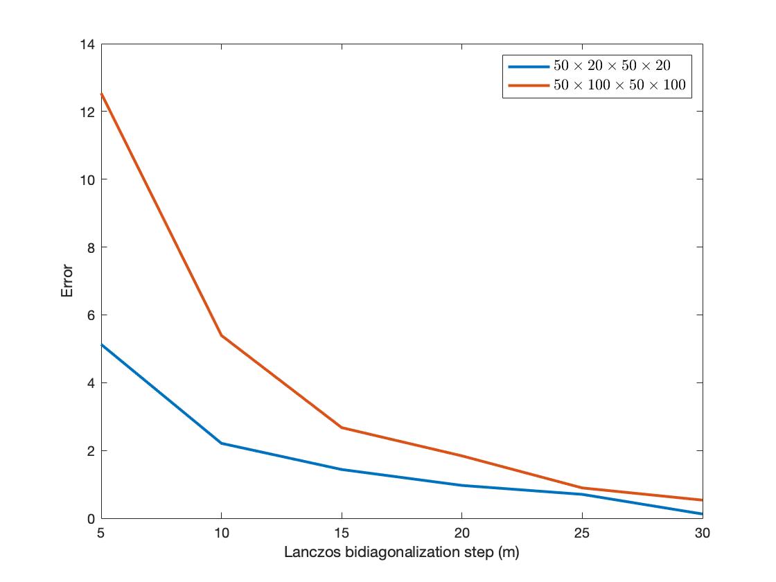
Figure 1: The error norm $\beta_{m}\left|u_{1}(m)\right|$ for different values of $m$.

From Figure 1, it can be observed that when the number $m$ of Lanczos bidiagonalization gets larger, the error decreases.

5.1.2 Ritz augmentation.

In this part, the numerical results of some tests on synthetic data are illustrated. These tests are carried out by using the Ritz augmentation process to approximate a desired number of tensor singular triplets (this number is denoted by $k$), for some chosen values of Lanczos bidiagonalization step $m>k$. In the sequel, the $i$-th approximated singular value is denoted by $\widetilde{s}_{i}$, while the exact one is denoted by $s_{i}$.

Approximation of the first singular triplets
This part is devoted to the approximation of the first (largest) singular triplets of synthetic tensors using the Ritz augmentation process.
In Table 4, the values of Res.norm are given when using the Ritz process to approximate the first four singular triplets of tensors for different tensor sizes, and by using $m=15$. Table 5 shows the error between the approximated singular values and the exact ones.

size($\mathcal{A}$)	$100\times 100\times 50$	$50\times 20\times 50\times 20$	$50\times 100\times 50\times 100$	$50\times 20\times 10\times 50\times 20\times 10$
$i=1$	1.77e-13	1.54e-13	6.55e-13	3.56e-12
$i=2$	2.98e-13	1.76e-13	1.95e-12	2.16e-12
$i=3$	2.26e-13	1.99e-13	1.74e-12	1.28e-12
$i=4$	1.49e-13	2.21e-13	4.90e-13	1.19e-12

Table 4: The Res.norm of each of the approximated singular triplets when using Ritz augmentation for $m=15$ and $k=4$.

size($\mathcal{A}$)	$100\times 100\times 50$	$50\times 20\times 50\times 20$	$50\times 100\times 50\times 100$	$50\times 20\times 10\times 50\times 20\times 10$
$i=1$	2.84e-14	2.13e-13	5.68e-14	4.26e-13
$i=2$	3.12e-13	1.98e-13	8.52e-13	7.95e-13
$i=3$	1.98e-13	9.94e-14	1.42e-13	5.40e-13
$i=4$	8.52e-14	7.64e-11	2.84e-10	1.17e-09

Table 5: The values of $\left|\widetilde{s}_{i}-s_{i}\right|$ of each of the approximated singular triplets when using Ritz augmentation for $m=15$ and $k=4$.

Table 6, presents the GRes.norm for different tensors when the first four singular triplets are approximated using the Ritz process with $m=15$. Tables 7 shows the influence of $m$ (Lanczos bidiagonalization step) on the GRes.norm and the number of iterations (Iter), when the first four singular triplets are desired to be approximated.

size($\mathcal{A}$)	$100\times 100\times 50$	$50\times 20\times 50\times 20$	$50\times 100\times 50\times 100$	$50\times 20\times 10\times 50\times 20\times 10$
GRes.norm	4.40e-13	7.57e-13	5.37e-12	1.75e-11

Table 6: The GRes.norm of the approximated first singular triplets when using Ritz augmentation for $m=15$ and $k=4$.

size($\mathcal{A}$)	$100\times 100\times 50$		$50\times 20\times 50\times 20$		$50\times 100\times 50\times 100$
	GRes	Iter	GRes	Iter	GRes	Iter
$m=5$	1.63e-12	107	4.63e-11	1000	1.84e-10	1000
$m=10$	9.40e-13	13	2.98e-12	45	9.99e-12	86
$m=15$	4.40e-13	5	7.57e-13	11	5.37e-12	19
$m=20$	7.85e-13	3	8.54e-13	6	4.08e-12	11

Table 7: The values of the GRes.norm and the number of iterations, when using Ritz augmentation with $k=4$ and $m=5,10,15,20$.

Figure 2 illustrates the error norm as defined in (7) on the first three singular triplets of the tensor of size $50\times 20\times 50\times 20$ for $m=15$.

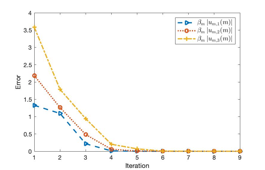
Figure 2: The error norm on each of the approximated first three singular triplets of the tensor of size $50\times 20\times 50\times 20$ when $m=15$.

Figure 2 show that the considered singular values are accurately approximated after just a few iterations.

Approximation of the last singular triplets

In this part, let us assume that a tensor admits $k_{max}$ singular triplets. Table 8 shows the Res.norm when approximating the last four singular triplets with $m=15$. Table 9 represents the error between the approximated singular triplets and the exact ones, when $m=15$ and $k_{max}=4$.

size($\mathcal{A}$)	$100\times 100\times 50$	$20\times 10\times 20\times 10$	$50\times 20\times 50\times 20$
$k=k_{max}-3$	2.37e-13	5.24e-14	2.91e-12
$k=k_{max}-2$	2.11e-13	6.75e-14	2.66e-12
$k=k_{max}-1$	1.69e-13	4.64e-14	1.60e-12
$k=k_{max}$	1.02e-13	2.76e-14	1.26e-12

Table 8: The Res.norm of each of the approximated last singular triplets when using Ritz augmentation for $m=15$ and $k_{max}=4$.

size($\mathcal{A}$)	$100\times 100\times 50$	$20\times 10\times 20\times 10$	$50\times 20\times 50\times 20$
$k=k_{max}-3$	7.10e-14	1.12e-12	1.18e-10
$k=k_{max}-2$	2.13e-13	1.11e-13	2.11e-13
$k=k_{max}-1$	$<$machine eps.	8.30e-13	4.05e-14
$k=k_{max}$	4.26e-14	1.45e-16	3.67e-14

Table 9: The error between the approximated singular values $\widetilde{s}_{i}$ and the Exact ones $s_{i}$; $\left|\widetilde{s}_{i}-s_{i}\right|$ for $i=1,2,3,4$ when $m=15$.

In Table, 10, the Gres.norm, the cpu-time, and the number of Iterations are illustrated, when the last four singular triplets are approximated, for $m=20\mbox{ and }30$. Figure 3 depicts the error used to accept the three last approximated singular triplets versus the number of iterations when $m=15$ on a $50\times 20\times 50\times 40$ tensor.

size($\mathcal{A}$)	$100\times 100\times 50$			$20\times 10\times 20\times 10$			$50\times 20\times 50\times 20$
	GRes.norm	cpu-time	Iter	GRes.norm	cpu-time	Iter	GRes.norm	cpu-time	Iter
$m=20$	4.17e-13	6.74	3	2.63e-13	10.87	102	3.91e-12	259.59	1000
$m=30$	3.74e-13	6.62	2	2.02e-13	7.13	37	8.88e-12	486.15	930

Table 10: The GRes.norm, the cpu-time, and the number of Iterations (Iter) for $k=4$ and $m=20,30$.

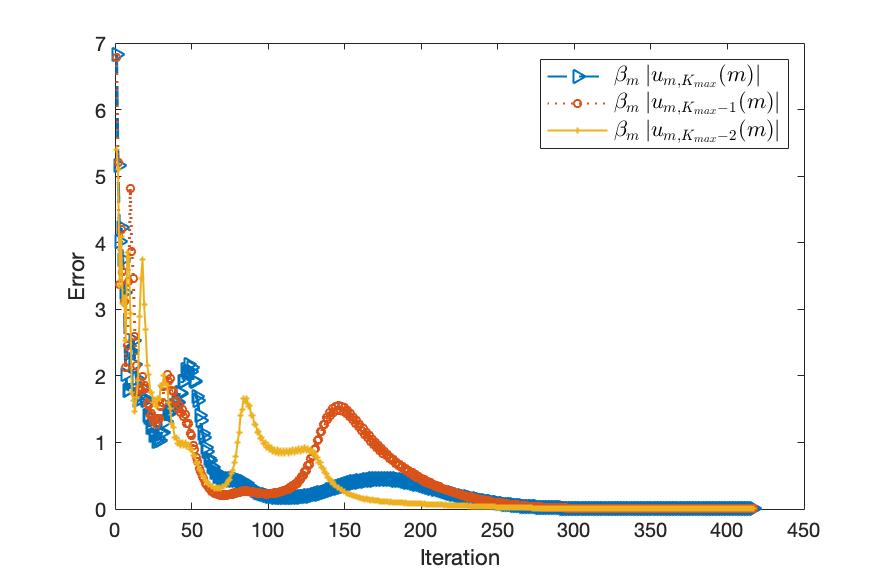
Figure 3: The error norm used to accept the last singular triplets when $k=3$ and $m=40$ on the tensor of size $50\times 20\times 50\times 20$.

5.2 Tensor compression

In this subsection, Algorithms 1 and 3 are applied to tensor compression. Algorithms 1 and 3 are denoted as LB, and Ritz, respectively. The tests are carried out on color videos which are stored as fourth-order tensors. The tests are performed on the videos obtained from Matlab files : xylophone of size $72\times 96\times 3\times 141$ and departure of size $72\times 108\times 3\times 337$. To measure the quality of the compressed data, the relative error norm defined as follows is used

$$\text{Relative error}=\dfrac{\left\|\mathcal{A}-\mathcal{A}_{k}\right\|_{F}}{\left\|\mathcal{A}\right\|_{F}},$$

where $\mathcal{A}$ is the tensor representing the data, and $\mathcal{A}_{k}=\sum_{i=1}^{k}\widetilde{s}_{k}\widetilde{\mathcal{U}}_{k}*_{2}\widetilde{\mathcal{V}}_{k}^{T}$, with $\{\widetilde{s}_{i},\widetilde{\mathcal{U}}_{i},\widetilde{\mathcal{V}}_{i}\}_{i=1}^{k}$ are the first approximated $k$ singular triplets of $\mathcal{A}$.
Figure 4 shows the $40$th bound of each the videos xylophone and departure, with the $40$th bounds of each of the compressed videos, with $k=10,20,30$, by using Ritz method with $m=40$.

Original	$k=10$	$k=20$	$k=30$

Figure 4: The $40$-th bounds of the compressed videos xylophone and departure by using Ritz method for $k=10,20,30$ with $m=40$.

Figure 5 depicts the values of the relative error norm against the values used of truncation ($k$) by using Ritz method and LB method, for both the videos xylophone and departure, respectively from the left to the right.

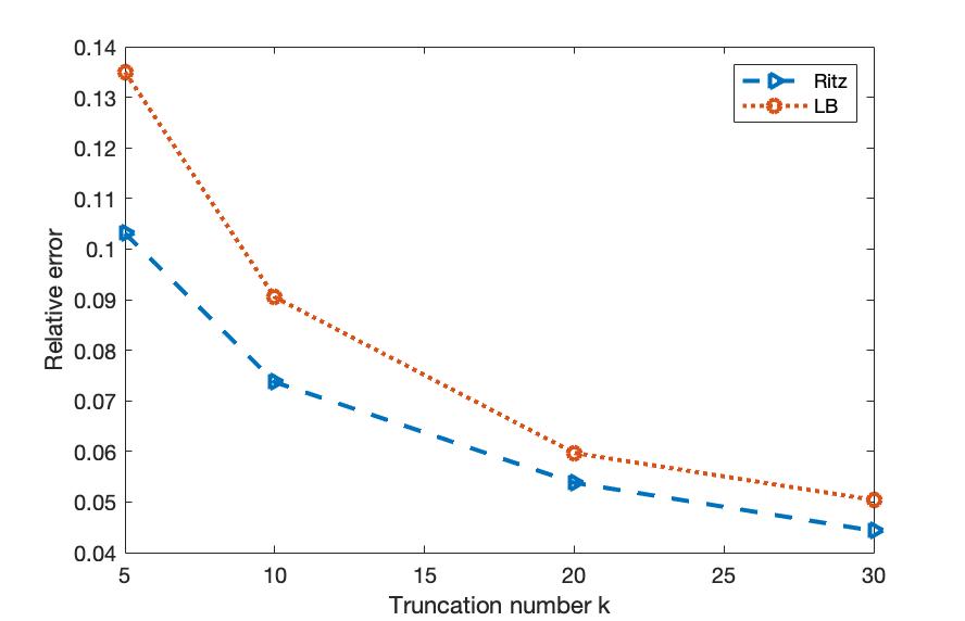
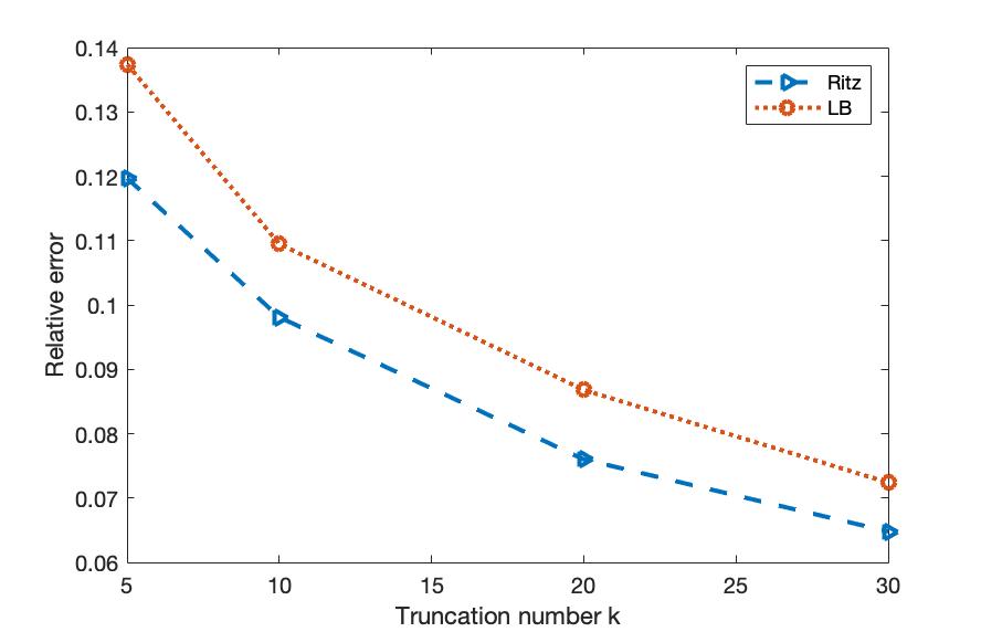
Figure 5: The relative error norm of the videos xylophone and departure, respectively from the left to the right, by using Ritz and LB methods.

Figure 4 and 5 illustrate the effectiveness of both methods for image compression, with a slight advantage to the Ritz methods.

5.3 Facial recognition based on the Einstein product

In this part, we illustrate some tests of facial recognition based on the Einstein product by using Algorithm 4. We refer to the tests performed with Algorithm 1 as LB, and to those using Algorithm 3 as Ritz.
The used data is obtained from the Georgia Tech database GTDB crop [22]. This database features the pictures of $50$ people. Each person is represented by $15$ pictures, each of which showing different facial expressions, illumination conditions, and orientation.
Each image is of size $50\times 50\times 3$. These two tests are carried out:

• Test 1: Five images of each person are randomly extracted from the database and are chosen as test images. Consequently, the database is split into two subsets : $250$ test images and $500$ training images used to form the training tensor $\widebar{\mathcal{X}}$ is of size $2500\times 3\times 500$.

• Test 2: $3$ pictures of each person are chosen randomly as test images. The remaining $600$ images are considered as the training images. The tensor $\widebar{\mathcal{X}}$ is of size $2500\times 3\times 600$.

The performance of both methods is measured by the identification rate (IR)

$$IR=\dfrac{\text{Number of recognized images}}{\text{Number of test images}}\times 100.$$

In Figure 6, we displayed one test image, the mean image and the closest image found in the database by using the Ritz method for Test 1, with $k=5$. In Figure 7 we illustrate the curves of the Identification Rate ($IR$) against the truncation index $(k)$ for Test 2, by the method using the exact Einstein SVD to compute the projection space called ”Exact”, the LB method, and the Ritz method.

Test image	Closest image	Mean

Figure 6: A result of Test 1 for truncation index $k=5$.

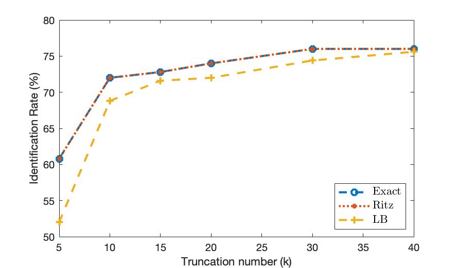
Figure 7: The curves of the identification rate (IR) versus the number of truncations used $k$, for the exact method and the approximated applied on Test 1.

In Table 11, the cpu-time is shown for the Exact, The LB, and the Ritz methods, when Test 1 and Test 2 are considered.

Test	Method	5	10	20	40
Test 1	Exact	295.48	298.93	307.42	298.50
	Ritz	57.41	66.01	74.97	123.80
	LB	49.57	54.64	61.97	82.98
Test 2	Exact	186.30	208.21	202.02	220.93
	Ritz	42.66	45.06	57.14	97.59
	LB	37.94	35.77	40.25	52.94

Table 11: The cpu-time required by the exact, the LB, and the Ritz methods for the PCA process, with different values of truncation $k=5,10,20,40$, for Test1 and Test 2.

While both methods showed to perform well in terms of identification rate, we notice that the Ritz method maintains an advantage over the LB method, especially for low rank approximations, which is particularly interesting for some applications including facial recognition for which the tensor can be very large and only a few singular triplets are needed. As expected, they required less CPU-time than the Exact Einstein SVD without affecting the accuracy, with an advantage for the LB method.

6 Conclusion

This paper presents an approach for approximating an extremal subset of singular triplets of a tensor using the Einstein product, regardless of its dimensionality. This approach, based on the Tensor Einstein Lanczos bidiagonalization and Ritz augmentation is particularly adapted to problems for which the computation of the complete SVD decomposition would be very time consuming. Numerical experiments show the effectiveness of this approach in terms of accuracy and CPU-time.

References

- [1] S. Aeron, E. Kernfeld, M. Kilmer, Tensor–tensor products with invertible linear transforms, Linear Algebra and its Applications, 485, 545–570, (2015).
- [2] M. N. Asif, I. S. Bajwa, S. I. Hyder, M. Naweed, Feature based image classification by using principal component analysis, ICGST Int. J. Graph. Vis. Image Process. GVIP, 9, 11–17, (2009).
- [3] H. Avron, L. Horesh, M. E. Kilmer, E. Newman, Tensor-tensor algebra for optimal representation and compression of multiway data, Proceedings of the National Academy of Sciences, National Acad Sciences, 188(28), e2015851118, (2021).
- [4] J. Baglama, L. Reichel, Augmented implicitly restarted Lanczos bidiagonalization methods, SIAM Journal on Scientific Computing, 27(1), 19–42, (2005).
- [5] B. W. Bader, T. Kolda, Tensor decompositions and applications, SIAM Review, 51(3), 455–500, (2009).
- [6] F. P. A. Beik, M. El Guide, A. El Ichi, K. Jbilou, Tensor Krylov subspace methods via the Einstein product with applications to image and video processing, Applied Numerical Mathematics, 181, 347–363, (2022).
- [7] A. H. Bentbib, A. EL Hachimi, K. Jbilou, A. Ratnani, A tensor regularized nuclear norm method for image and video completion, Journal of Optimization Theory and Applications, 192(2), 401–425, (2022).
- [8] A. H. Bentbib, A. El Hachimi, K. Jbilou, A. Ratnani, Fast multidimensional completion and principal component analysis methods via the cosine product, Calcolo, 59(3), 26, (2022).
- [9] A. H. Bentbib, A. Khouia, H. Sadok, Color image and video restoration using tensor CP decomposition, BIT Numer. Math., 62(4), 1257–1278, (2022).
- [10] A. H. Bentbib, M. Elalj, A. El Hachimi, K. Jbilou, A. Ratnani, Generalized L-product for high order tensors with applications using GPU computation, arXiv preprint arXiv:2202.02870, (2022).
- [11] K. Braman, N. Hao, R. C. Hoover, M. E. Kilmer, Third-order tensors as operators on matrices: A theoretical and computational framework with applications in imaging, SIAM Journal on Matrix Analysis and Applications, 34(1), 148–172, (2013).
- [12] M. Brazell, N. Li, C. Navasca, C. Tamon, Solving multilinear systems via tensor inversion, SIAM Journal on Matrix Analysis and Applications, 34(2), 542–570, (2013).
- [13] C. Bu, L. Sun, Y. Wei, B. Zheng, Moore–Penrose inverse of tensors via Einstein product, Linear and Multilinear Algebra, 64(4), 686–698, (2016).
- [14] A. Einstein, The foundations of the general theory of relativity In The Collected Papers of Albert Einstein, Volume 6: The Berlin Years: Writings, 1914–1917, English Translation Supplement, 146–200, (1997).
- [15] M. El Guide, K. Jbilou, A. Ratnani , RBF approximation of three dimensional PDEs using tensor Krylov subspace methods, Engineering Analysis with Boundary Elements, 139, 77–85, (2022).
- [16] A. El Hachimi, K. Jbilou, A. Ratnani, L. Reichel, A tensor bidiagonalisation method for higher-order singular value decomposition with applications, NLA, (2023).
- [17] A. El Hachimi, K. Jbilou, A. Ratnani, L. Reichel, Spectral computation with third-order tensors using the t-product, Applied Numerical Mathematics, 193, 1–21, (2023).
- [18] G. H. Golub , C. F. Van Loan, Matrix Computations, The Johns Hopkins University Press, (2013).
- [19] M. Hached, K. Jbilou, C. Koukouvinos, M. Mitrouli, A multidimensional principal component analysis via the C-product Golub–Kahan–SVD for classification and face recognition, Mathematics, 9(11), 1249, (2021).
- [20] M. E. Kilmer, C. D. Martin, Factorization strategies for third-order tensors, Linear Algebra and its Applications, 435(3), 641–-658, (2011).
- [21] B. LaRue, C. Martin, R. Shafer, An order-p tensor factorization with applications in imaging, SIAM Journal on Scientific Computing, 35(1), A474–A490, (2013).
- [22] A.V. Nefian, Georgia Tech Face Database, Available online: http://www.anefian.com/research/face_reco.htm.
- [23] P. K. Pandey, Y. Singh, S. Tripathi, Image processing using principle component analysis, International Journal of Computer Applications, 15(4), 37–40, (2011).