Longitudinal polaritons

Abstract

The collective excitations of solids are classified as longitudinal and transverse depending on their relative polarization and propagation direction.^{1; 2} This seemingly subtle difference results in surprisingly distinct types of excitations if calculated within the Coulomb gauge. Transverse modes couple to free-space photons and hybridize into polaritons for strong light-matter coupling.^{3; 4; 5} Longitudinal modes, in contrast, are seen as pure matter excitations that produce a dynamic polarization inside the material. Here we show that both longitudinal and transverse modes become polaritons in the explicitly covariant Lorenz gauge.^{6; 7} Longitudinal excitations couple to longitudinal and scalar photons, which have been considered elusive so far. We show that the dipolar excitations become three-fold degenerate in the long-wavelength limit when including all photonic degrees of freedom, as expected from symmetry.^{8; 9} Our findings demonstrate how choosing a gauge determines our thinking about materials excitations and how gauge fixing reveals new pathways for tailoring polaritons in crystals, metamaterials, and surfaces. Longitudinal polaritons will interact with longitudinal near fields located at surfaces, which provides additional excitation channels in scanning near-field microscopy and surface-enhanced spectroscopy.¹⁰

Condensed-matter theory describes the dielectric response of materials by collective dipole excitations that get induced by electric fields.^{1; 2} This concept models optically active excitations of electrons, phonons, excitons, plasmons, and other quasiparticles;¹¹ it explains the electrical susceptibility and dielectric function from the far infrared to the visible and soft X-ray regime.¹ The collective dipole excitations are usually divided into two distinct types: the longitudinal - parallel polarization and propagation directions - and the transverse - polarization and propagation directions are perpendicular. This separation is convenient in the Coulomb gauge, where only the transverse modes interact with the transverse electromagnetic field of propagating photons. Their interaction leads to the formation of hybrid light-matter states or polaritons for strong enough light-matter coupling.^{4; 5} The longitudinal modes, on the other hand, are regarded as pure matter excitations and uncoupled to photons, for example, a longitudinal phonon is understood mainly as a mechanical wave.^{4; 2}

Modeling dipolar longitudinal and transverse modes as fundamentally different results in contradictions that have not been resolved so far.^{9; 4; 8; 2} Cohen and Keffer showed in a seminal paper that the longitudinal frequency $\omega_{l}$ is higher for vanishing wavevector $\mathbf{k}$ than the corresponding transverse excitation $\omega_{t}$.⁹ This well-known logitudinal-transverse (LT) splitting appears unphysical since the propagation direction becomes ill defined for $k=0$. Several proposals attempted to consolidate LT splitting with our general understanding of crystals,^{8; 2; 9} most convincingly, by including retardation or light-matter interaction.^{3; 4} When adding light-matter coupling to the crystal Hamiltonian, the upper transverse polariton at $\Gamma$ systematically coincides with the longitudinal dipole mode. While this solves the discrepancy for the eigenenergies, it also suggests a degeneracy between two different types of excitations, the transverse polaritons and the longitudinal matter mode. A systematic degeneracy appears impossible for the regimes of ultrastrong and deep strong light-matter coupling regime where the upper transverse polariton is almost exclusively composed of photons with vanishing contribution of matter excitations,^{12; 13; 14} while the longitudinal mode remains a pure matter state. ^{3; 4}

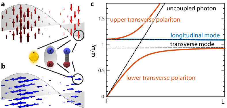
Figure 1: Induced dipoles and their dispersion. Sketch of the (a) transverse and (b) longitudinal collective modes. The dipoles may be associated with various material excitations, e.g., plasmons, excitons, and phonons. c Polariton dispersion along the $\Gamma L$ direction of a face centered cubic lattice calculated in the Coulomb gauge. Dashed lines represent the longitudinal and transverse modes without light-matter coupling.

Here we show that in the Lorentz gauge the longitudinal and transverse dipole excitations are indistinguishable in the long wavelength limit, thus challenging the well established concept that only transverse excitations form polaritons. While the transverse modes continue to couple to transverse photons, the longitudinal modes couple to longitudinal and scalar photons making them also hybrid light-matter states. We show that the longitudinal and transverse polaritons are systematically degenerate at $k=0$; the apparent LT splitting arose from an inconsistent treatment of light-matter coupling in the Coulomb gauge. Describing longitudinal and transverse modes as polaritons unifies our understanding of material excitations. It widens the choice of excitations for near-field optics and polariton devices by adding longitudinal polaritons as hybrid states of longitudinal and scalar photons with dipolar matter modes.

To describe materials excitations and their coupling to light we consider a lattice of isotropic bosonic dipole excitations with frequency $\omega_{0}$, Fig. 1a and b, coupled to the free electromagnetic field. These excitations represent the localized contribution to crystal phonons, excitons, plasmons, spin waves, and so forth.¹¹ The coupled light-matter system is described by a semi-empirical Hamiltonian

$$\mathcal{H}_{\mathrm{LM}}=\mathcal{H}_{mat}+\mathcal{H}_{EM}+\mathcal{H}_{int}.$$ (1)

The matter part of the Hamiltonian is given by

$$\mathcal{H}_{mat}=\sum_{\mathbf{k}}\omega_{0}b_{j,\mathbf{k}}^{\dagger}b_{j,\mathbf{k}},$$ (2)

where $b_{j,\mathbf{k}}^{\dagger}=1/N\sum_{n}b_{j,n}^{\dagger}(\mathbf{r}_{n})\exp(i\mathbf{k}\cdot\mathbf{r}_{n})$ and $b_{j,n}^{\dagger}(\mathbf{r}_{n})$ creates a dipole excitation at site $\mathbf{r}_{n}$ and polarized along the $j$ direction ($j=x,y,z$), $N$ is the total number of lattice sites. When treating $\mathcal{H}_{\mathrm{LM}}$ within the Coulomb gauge the dipole-dipole interaction between the localized excitations leads to longitudinal and transverse eigenstates, dashed lines in Fig. 1c, that are understood as the pure crystal excitations. Their coupling to propagating photons results in the transverse lower and upper polariton, orange lines in Fig. 1c, whereas the longitudinal mode remains unaffected by light-matter coupling, blue line in Fig. 1c.

To switch to the Lorenz gauge we write the photon in the covariant form ($c=\hbar=1$)

$$\mathcal{H}_{EM}^{\rm LG}=\int d^{3}k\sum_{j}k[a_{j,\mathbf{k}}^{\dagger}a_{j,\mathbf{k}}-a_{0,\mathbf{k}}^{\dagger}a_{0,\mathbf{k}}],$$ (3)

where $a_{j}$ is the annihilation operator for the vector potential $\mathbf{A}_{j}$ and $a_{0}$ for the scalar potential $A_{0}(\mathbf{k})=\rho(\mathbf{k})$. Since the dipole displacement is small compared to the lattice constant $a$ the interaction Hamiltonian is, Methods,

$$\begin{split}\mathcal{H}_{int}^{\mathrm{LG}}(\mathbf{k})=&\sum_{j,j^{\prime},\mathbf{G}}\frac{g^{2}\xi^{2}}{\omega_{0}}(\hat{e}_{j}\cdot\hat{e}_{j^{\prime}})[(a_{j,\mathbf{k}}+a_{j,-\mathbf{k}}^{\dagger})(a^{\dagger}_{j^{\prime},\mathbf{k}+\mathbf{G}}+a_{j^{\prime},-\mathbf{k}-\mathbf{G}})]+\\ +&ig\xi(\hat{e}_{j}\cdot\hat{e}_{j^{\prime}})[(b_{j,\mathbf{k}}-b_{j,-\mathbf{k}}^{\dagger})(a^{\dagger}_{j^{\prime},\mathbf{k}+\mathbf{G}}+a_{j^{\prime},-\mathbf{k}-\mathbf{G}})]+\\ +&ig\frac{\hat{e}_{j}\cdot\hat{n}_{\mathbf{k}+\mathbf{G}}}{\xi}[(b_{j,\mathbf{k}}-b_{j,-\mathbf{k}}^{\dagger})(a^{\dagger}_{0,\mathbf{k}+\mathbf{G}}+a_{0,-\mathbf{k}-\mathbf{G}})],\end{split}$$ (4)

where $\xi=\sqrt{\omega_{0}/|\mathbf{k}+\mathbf{G}|}$, $\hat{n}_{\mathbf{k}+\mathbf{G}}$ is a unit vector along the $\mathbf{k}+\mathbf{G}$ direction and $V$ is the volume of the unit cell. $\mathbf{G}$ runs over all reciprocal lattice vectors. $g=\sqrt{q^{2}/4mV}$ is the light-matter coupling strength of the excitation. The full interaction Hamiltonian follows by summing all three directions in space. $\hat{e}_{j}$ is the polarization direction for the photon or the dipole with wavevector $\mathbf{k}$ and $\hat{e}_{j^{\prime}}$ for the states with $\mathbf{k}+\mathbf{G}$.

In the Lorenz gauge $\mathcal{H}_{LM}$ is highly symmetric for transverse and longitudinal photon excitations. The matter $\mathcal{H}_{mat}$ and photon part $\mathcal{H}_{EM}^{\mathrm{LG}}$ as well as the coupling of the local dipoles to transverse and longitudinal photons, first two terms in $\mathcal{H}_{int}^{\mathrm{LG}}$, are independent of propagation direction. The longitudinal and transverse solutions are, therefore, identical when we neglect scalar photons, third term in Eq. (4). The term is only present for longitudinal modes, i.e., if the polarization is parallel to the propagation direction and vanishes for $k=0$. Any solutions of $\mathcal{H}_{LM}$ will be three-fold degenerate at $\Gamma$ and all eigenvectors are polaritons or coupled light-matter states.

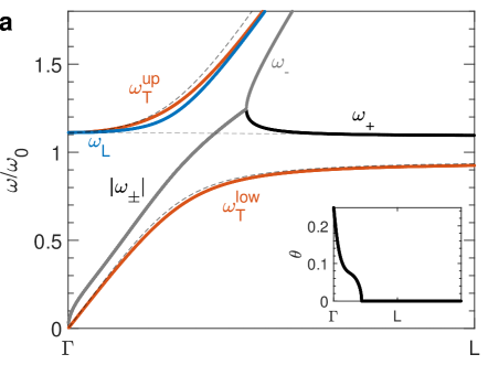
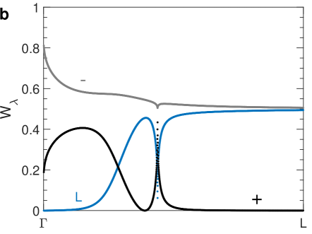
Figure 2: a Dispersion of the transverse (red) polariton, and longitudinal (blue, black and gray) solutions. The inset shows the phase ($\theta$) of the longitudinal modes for a diagonalization by a similarity transformation (see text for detail). b Relative contribution ($W_{\lambda}=|Z_{\lambda}|^{2}/\sum|Z_{\lambda}|^{2}$) of the longitudinal modes to the subsidiary condition. Only states with $Z_{\lambda}\approx 0$ can be considered as physical states. $g/\omega_{0}=0.25$, $a\omega_{0}=\pi/3$. The dashed line in a corresponds to the calculation in the Coulomb gauge.

The Lorenz gauge introduces four degrees of freedom for the electromagnetic field (two transverse, one longitudinal, and one scalar), but two of these degrees of freedom must be removed when solving the Hamiltonian. This is done by imposing subsidiary conditions; excitations that violate the condition remain unpopulated at all times.^{15; 7} To properly describe hybrid light and matter excitations, we must search for a set of operators $\psi_{\lambda,\mathbf{k}}$ and $\psi_{\lambda,\mathbf{k}}^{\dagger}$ that fulfill the following conditions

$$i\frac{d}{dt}\psi_{\lambda,\mathbf{k}}=[\psi_{\lambda,\mathbf{k}},\mathcal{H}]=\omega_{\lambda,\mathbf{k}}\psi_{\lambda,\mathbf{k}},$$ (5a)

$$[\psi_{\lambda,\mathbf{k}},\psi_{\lambda^{\prime},\mathbf{k}}^{\dagger}]=\pm\delta_{\lambda\lambda^{\prime}},\text{and}$$ (5b)

$$Z_{\lambda}(\mathbf{k})\psi_{\lambda,\mathbf{k}}|\chi\rangle=0,$$ (5c)

where $[~{}]$ is the commutator. Condition (5a) requires the solutions to be linearly independent and Condition (5b) ensures canonical (or anti-canonical) commutation relations. The negative sign is included because of the anti-hermitian nature of the scalar potential $[a_{0,\mathbf{k}},a_{0,\mathbf{k}}^{\dagger}]=-1$.¹⁶ Condition (5c) imposes the Lorentz gauge. Here, $|\chi\rangle$ is an appropriately defined Fock state and $Z_{\lambda}(\mathbf{k})$ weights the contribution of $\psi_{\lambda,\mathbf{k}}$ to the subsidiary condition, see methods for details. Operators $\psi_{\lambda,\mathbf{k}}$ for which $Z_{\lambda}(\mathbf{k})$ is non-zero require that $\psi_{\lambda,\mathbf{k}}|\chi\rangle$ vanishes at all times for all physically relevant states, thus being removed from the dynamics of the system. Ideally, two sets of operators will be eliminated through this process, thus effectively reestablishing the expected two degrees of freedom.

The peculiar commutation relation of the scalar photon operator requires that we define a generalized Bogoliubov-Valantin (BV) transformation to attempt diagonalizing the dynamical matrix, see discussion in Methods. We define these as the set of linear transformations that map the creation and annihilation operators of the bare excitations onto the set of operators $\psi_{\lambda,\mathbf{k}}$ that describe the interacting system while conserving the commutation relations. To properly solve the problem at hand, we separated the Hamiltonian $\mathcal{H}_{\mathrm{LM}}$ into its longitudinal and transverse part, restricted the wavevectors to $\mathbf{G}=0$, and included the coupling to the $\mathbf{G}\neq 0$ longitudinal and scalar photons as a self-energy correction to the dipole energy, see Methods. The transverse part of the dynamical matrix is diagonalized by a regular BV transformation yielding two physically acceptable hybrid light-matter states, or polaritons, full red and grey lines in Fig. 2a. They are close in energy to the transverse solutions in the Coulomb gauge, dashed lines. The remaining discrepancies arise from disregarding the wavevector dependence of the self-energy correction, see methods.

The longitudinal part of the Hamiltonian involves the interaction of the dipoles with longitudinal and scalar photons and cannot be solved trivially. To circumvent this, we first diagonalized the dynamical matrix numerically by conjugation to obtain the eigenfrequencies $\omega_{L,\mathbf{k}}$, $\omega_{+,\mathbf{k}}$, and $\omega_{-,\mathbf{k}}$ in Fig. 2(a). $\omega_{L,\mathbf{k}}$ is real, grey and blue line in Fig. 2a, while the set ($\omega_{+,\mathbf{k}}$, $\omega_{-,\mathbf{k}}$) has the characteristics of non-hermitian parity-time symmetric Hamiltonians, such as the presence of an exceptional point $k_{\mathrm{EP}}$. ^{17; 18} The eigenspectrum includes two complex frequencies $\omega_{+,\mathbf{k}}=\omega_{-,\mathbf{k}}^{\dagger}=\omega_{\pm}e^{\pm i\theta}$ for $k<k_{\mathrm{EP}}$ and two real frequencies $\omega_{+,\mathbf{k}}\neq\omega_{-,\mathbf{k}}$ for $k>k_{\mathrm{EP}}$, grey-blue-yellow lines in Fig. 2a. Although diagonalizing numerically by conjugation gave us the eigenfrequencies, it does not allow for describing the solutions as creation and annihilation operators, which we need to identify the physically relevant states. For this, we apply the proposed a generalized BV transformation that partially diagonalizes the Dynamical matrix, leading to one fully independent solution with the same eigenenergy $\omega_{L,\mathbf{k}}$ and two coupled solutions, $\psi_{+,\mathbf{k}}$ and $\psi_{-,\mathbf{k}}$. The operator $\psi_{L}$ obeys the three Conditions (5) close to the $\Gamma$ point as $Z_{\mathbf{k},L}$ vanishes as $k^{2}$. It is a composition of bare longitudinal dipoles and longitudinal and scalar photons and represents the physical excitations of the system with independent dynamics. In contrast, $Z_{\mathbf{k},+}$ and $Z_{\mathbf{k},-}$ are non-zero close to $\Gamma$ and do not correspond to physical excitations, Fig. 2b, i. e., these linearly dependent excitations must thus remain unpopulated in any physically relevant state.

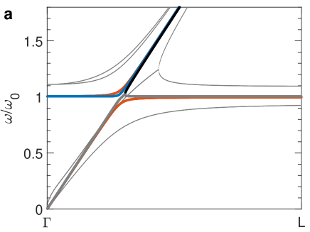
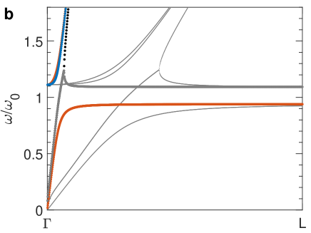
Figure 3: Polariton dispersion for two different sets of parameters: a $g/\omega_{0}=0.05$ and $a\omega_{0}=\pi/3$ and b $g/\omega_{0}=0.25$ and $a\omega_{0}=\pi/20$. For comparison, the dispersion of Fig. 2 ($g/\omega_{0}=0.25$ and $a\omega_{0}=\pi/3$) is shown in thin grey lines. The polaritons are colored according to the relative contributions of the bare excitations. Transverse (TD) and longitudinal (LD) dipoles in grey, transverse (TP), longitudinal (LP) and scalar (SP) photons in red, blue and yellow, respectivelly. For weak coupling and/or small $a\omega_{0}$, the longitudinal polariton is mainly composed of dipole excitations (grey) for the most part of the Brillouin zone.

For small wavevectors the light-matter Hamiltonian within the Lorenz gauge leads to one physically relevant longitudinal polariton. It is degenerate with the two transverse upper polaritons at $k=0$. The degeneracy occurs independently of crystal structure and the magnitude of the light-matter coupling. We only assumed that the individual dipole excitations are isotropic meaning that the LT degeneracy is a general result. We also observed it systematically in binary dipole lattices with two independent dipole excitations of different frequencies.¹⁹ This finding, however, does not apply to low-dimensional systems: We can describe a free-standing two-dimensional layer as a three-dimensional crystal with one lattice vector taken to infinity or infinitely small reciprocal lattice vector. The $\mathbf{G}\neq 0$ terms remain relevant even for vanishing $k$ resulting in different self-energy corrections for the transverse and longitudinal modes, which lifts the LT degeneracy, see Methods. For three-dimensional crystals, we solved the vexing degeneracy between a hybrid light-matter and a pure matter state, e.g., a mechanical wave in the case of phonons, because both the transverse and the longitudinal branch are coupled matter-photon states. The upper polariton at $\Gamma$ becomes more and more photon-like with increasing light-matter coupling until photons dominate for $g\gtrsim 0.5\omega_{0}$, see Extended Data Figs. 1 and 2. The Lorenz gauge describes polaritons in the long-wavelength limit without using Ewald summation techniques nor producing discontinuities. It may also lead to an unambiguous description of static homogeneous polarization in crystals without resorting to Berry curvatures and phases, as suggested in the modern theory of polarization.²⁰

Although our model was motivated mainly by understanding material excitation close to $\Gamma$, we found it illuminating to look at the dispersion throughout the Brillouin zone. With increasing $k$ we reach a critical point at $k=k_{\mathrm{EP}}$ that separates the long-wavelength behavior close to $\Gamma$ from the short-wavelength behavior in the rest of the Brillouin zone, Fig. 2a. Exceptional points occur in the solutions of non-hermitian Hamiltonians.^{17; 18} None of the excitations are physically relevant at $k_{\mathrm{EP}}$, Fig. 2, because $Z_{L},Z_{+},$ and $Z_{-}$ are simultaneously different from zero, which means that our choice for fixing the gauge is inappropriate to describe the system at these $k$. The Lorenz gauge is not completely fixed, because the vector potentials may be shifted by $A_{L}\rightarrow A_{L}+\nabla f$ and $A_{0}\rightarrow A_{0}-\partial f/\partial t$ for a wide class of functions $f$. There should be a gauge fixing condition that results in physically relevant states for all wavevectors, which calls for further research to fully describe condensed-matter excitations in the Lorenz gauge. For $k>k_{\mathrm{EP}}$ and the coupling parameters used here, the contribution of the $\psi_{+}$ term ($Z_{+}$) decreases and $Z_{+}$ drops almost to zero at the $L$ point of the Brillouin zone, whereas $Z_{L}$ and $Z_{-}$ sharply increase in value. For large $k$, $Z_{+}$ describes the one physically relevant state of the system. The nearly flat longitudinal band in Fig. 2(a), black line, close to the zone edge coincides with the dispersion of the longitudinal mode in the Coulomb gauge, dashed lines, see Methods.

Decreasing the strength of light-matter coupling $g$ moves $k_{\mathrm{EP}}$ closer to $k=\omega_{0}$, where the photon and the dipole excitation have the same energy, Fig. 3a; increasing $g$ moves $k_{\mathrm{EP}}$ to larger $k$ so that it may cross the zone edge. The $\mathbf{G}\neq 0$ photons then interact resonantly with the excitations and need to be considered explicitly. Increasing $g$ also moves the exceptional point up in energy and increases the minimum separation $\Omega_{R}=2g$ between the upper and lower transverse polaritons, Fig. 3a. The second parameter governing the polariton dispersion is the lattice constant $a$ that moves the crossing point $k=\omega_{0}$ without affecting the Rabi frequency $\Omega_{R}$. The lattice constant of natural crystals are on the order of $a\sim 10^{-1}$ m and $a\cdot\omega_{0}<<1$ as for the simulation in Fig. 3b. In this case, both polariton branches are mainly matter like close to $\omega_{0}$, because the lower transverse polariton and the short-wavelength longitudinal polariton ($k>k_{\mathrm{EP}}$) are dominated by matter excitations.^{12; 13} Metamaterials and artificial supercrystals have $a\approx 10-1000\,$nm meaning that the crossing point $k=\omega_{0}$ occurs in the middle of the Brillouin zone, Fig. 2a. The photon-like part of the longitudinal mode will be more accessible in such engineered structures.

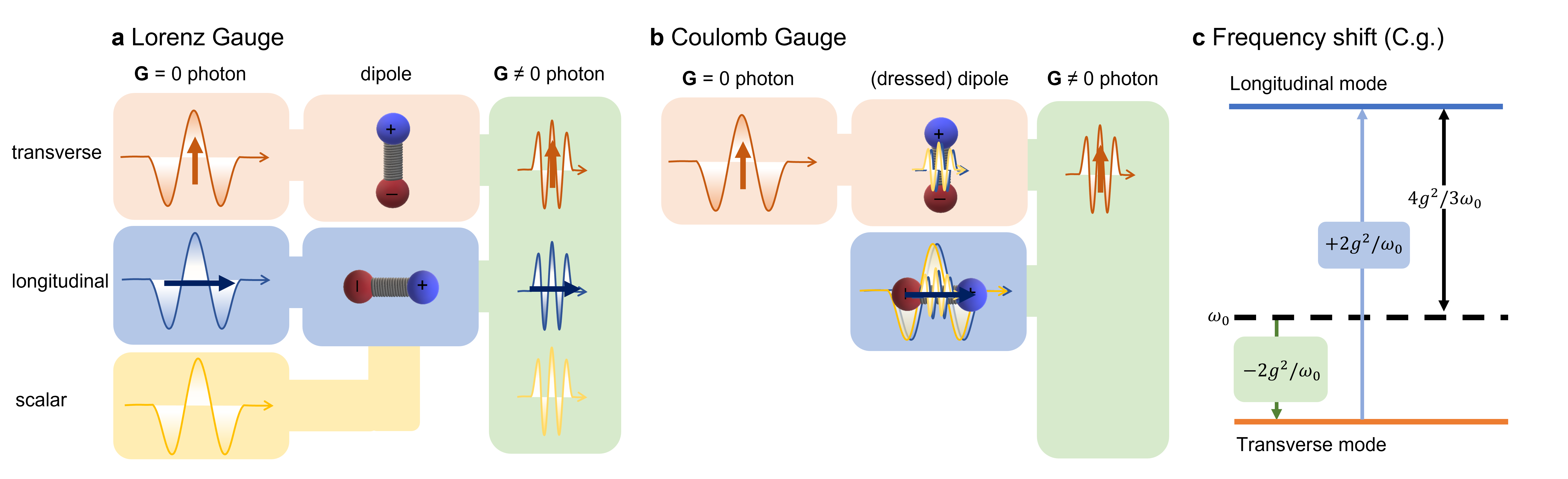
Figure 4: Light-matter coupling in the Lorenz and Coulomb gauge. a In the Lorenz gauge the long-wavelength transverse photons couple to transverse dipoles ($\mathbf{G}=0$, orange), long-wavelength longitudinal and scalar photons couple to longitudinal dipoles ($\mathbf{G}=0$, blue). All short wavelength photons couple to all dipoles ($\mathbf{G}\neq 0$, green). All components of light-matter coupling are treated explicitly; the dipoles remain undressed. b In the Coulomb gauge the long-and short-wavelength longitudinal and scalar photons dress the longitudinal dipoles. They become inseparable from the longitudinal mode that always has a photonic contribution (blue). The longitudinal and scalar short wavelength photons dress the transverse dipoles ($\mathbf{G}\neq 0$, green). The long-wavelength transverse photons couple to the transverse dipoles. The short wavelength transverse photons couple to both dipoles. Only the coupling to the transverse modes is treated explicitly. c Energy shifts in the Coulomb gauge due to the dressing by photons. Transverse and longitudinal modes shift down due to the inclusion of the short-wavelength photons (green). The longitudinal modes shift up through the long-wavelength longitudinal and scalar photons (blue). The transverse mode remains finite and at lower frequency when neglecting the coupling of the transverse modes.

It is fascinating to examine how the description of materials excitations in the Lorenz and Coulomb gauge shape our understanding of matter, Fig. 4. It may even lead to apparent gauge ambiguities similar to the ones observed in cavity electrodynamics for inconsistent approximations in the various gauges. ^{21; 22} In the Lorenz gauge the dipole excitations remain undressed. Their coupling to light is treated explicitly for all photons. All collective eigenstates are polaritons; the coupling of the longitudinal and transverse photons to matter is completely symmetric. In the Coulomb gauge the dynamical parts of some photons gets infused with the excitations creating dressed collective states that contain the photons in an inseparable way. All dipole excitations get dressed by the short-wavelength scalar and longitudinal photons, dressed dipole in Fig. 4b, reducing the frequency of the single dipole $\omega_{0}$ to the collective frequency, Fig. 4c. The longitudinal collective excitations are then dressed by the long-wavelength longitudinal and scalar photons increasing the longitudinal frequency to a net blue shift $+4g^{2}/3\omega_{0}$ compared to $\omega_{0}$, see Methods and Fig. 4b and c. This last step gets introduced in materials modeling as an electric field produced by the longitudinal excitations that results in an additional frequency term, e.g., the Born effective charge for phonons in ionic crystals. The transverse photons remain separate from the transverse dipole excitations in the Coulomb gauge. Only this coupling is made explicit in the so-called light-matter interaction term that may or may not be included in the calculation. The appearance of a transverse mode with non-zero frequency below $\omega_{0}$ at $\Gamma$ and the resulting LT splitting is a consequence of neglecting one part of light-matter interaction, namely the separable part related to the transverse mode, while including the inseparable part in the longitudinal mode that was incorrectly understood as a matter-only excitation.

Our point of view suggests an important shift in paradigm. By describing the longitudinal excitations in materials as hybrid light-matter states we allow for a deeper understanding of their physical properties within a quantum mechanical framework.This proposed shift is, however, much more than just a change of perspective. For instance, just as virtual longitudinal and scalar photons play an important role in describing the interaction between different charges in vaccum,¹⁶, the virtual polaritonic excitations in the Lorentz gauge may be useful for alternate quantum descriptions of the screened Coulomb interaction in materials. Also, longitudinal polaritons in the ultra-strong and deep-strong coupling regimes should experience similar physical effects as those predicted for the transverse polaritons, such as light-matter decoupling, vanishing Purcell effect, squeezed photons and virtual excitations in the ground state.^{12; 23} However, most experiments developed so far focus mainly on the transverse excitations. Recent developments in tayloring plasmonic and photonic structures to different energy ranges and spacial scales widen the path for studying these exquisite longitudinal polaritons and unravelling new related phenomena.

I Methods

I.1 Hamiltonian

The electromagnetic field, in units of $c=\hbar=1$, is written as

$$A_{\mu}(\mathbf{r},t)=\int d^{3}k\sqrt{\frac{1}{2k}}\left[a_{\mu}(\mathbf{k})e^{i(\mathbf{k}\cdot\mathbf{r}-\omega t)}+a^{\dagger}_{\mu}(\mathbf{k})e^{i(\mathbf{k}\cdot\mathbf{r}-\omega t)}\right].$$ (6)

where $\mu$ runs between 0 and 3, 0 being related to the scalar potential $A_{0}(x_{\mu})=\Phi(x_{\mu})$. The creation and annihilation operators for the vector potential obey cannonical commutation relations, the scalar potential has some exquisite properties: $(a_{0})^{\dagger}=-a_{0}^{\dagger}$ and $[a_{0},a_{0}^{\dagger}]=-1$. $a_{0}$ commutes with the other operators. Following the work of Babiker ^{24; 15; 7}, the hamiltonian for the electromagnetic field in the Lorenz gauge is

$$\mathcal{H}_{EM}^{\rm LG}=\int d^{3}k\sum_{j}k[a_{j}^{\dagger}(\mathbf{k})a_{j}(\mathbf{k})-a_{0}^{\dagger}(\mathbf{k})a_{0}(\mathbf{k})],$$ (7)

where $j$ runs over the three dimensions in space $x,y,z$. According to the Gupta-Bleuler^{15; 7} quantization formalism, the Lorenz condition is imposed by requiring that physical states are those for which

$$\left[a_{L}(\mathbf{k})-a_{0}(\mathbf{k})\right]|\chi\rangle=0,$$ (8)

where the $L$ (for longitudinal) is the direction parallel to $\mathbf{k}$.

We further assume that each site of a regular lattice holds an isotropic bosonic dipole-like excitation governed by the Hamiltonian

$$\mathcal{H}_{mat}=\sum_{n}\frac{p_{n}^{2}}{2m}-\frac{m\omega_{0}^{2}}{2}h_{n}^{2}=\sum_{n,j}\omega_{0}b_{j,n}^{\dagger}b_{j,n}$$ (9)

where $\mathbf{h}_{n}$ is the displacement of the $n$-th dipole and $\mathbf{p}_{n}$ it’s conjugate momentum. We left out the zero point energy.

The light-matter interaction is

$$\mathcal{H}_{int}^{\rm LG}=\sum_{n}\frac{q^{2}}{2m}A_{j}^{2}(\mathbf{r}_{n})+\frac{q}{m}\mathbf{p}_{n}\cdot\mathbf{A}(\mathbf{r}_{n})-\rho(r_{n})A_{0}(\mathbf{r}_{n}),$$ (10)

with $\mathbf{p}_{n}$ the momentum of the $n$-th dipole and $\rho(r)$ the charge distribution. Throughout this paper the vector notation $\mathbf{V}$ refers to vectors in 3D space.

The total hamiltonian in the Lorenz gauge is then $\mathcal{H}=\mathcal{H}_{EM}^{\rm LG}+\mathcal{H}_{mat}+\mathcal{H}_{int}^{\rm LG}$, where it is convenient to write the two last terms in the right-hand side in reciprocal space. For this, it is straight forward to define $\mathbf{p}(\mathbf{k})$ and $\mathbf{h}(\mathbf{k})$ as the Fourier transform of the real space quantities. We define the charge distribution for each dipole as that obtained by two opposite charges oscillating around their rest position at $\mathbf{r}_{n}$ with a total displacement of $\mathbf{h}_{n}$ - $\rho(\mathbf{r}_{n})=\sum_{n}q\int d^{3}r[\delta(\mathbf{r}-\mathbf{r}_{n}\mathbf{+}\mathbf{h}_{n}/2)-\delta(\mathbf{r}-\mathbf{r}_{n}\mathbf{-}\mathbf{h}_{n}/2)]$. With this the charge density in reciprocal space is

$$\begin{split}\mathbf{\rho}(\mathbf{k})=&\int d^{3}r\rho(\mathbf{r})\exp(i\mathbf{k}\cdot\mathbf{r})=2iq\sum_{n}\sin(\mathbf{k}\cdot\mathbf{h}_{n}/2)\exp(i\mathbf{k}\cdot\mathbf{r}_{n})\\ \sim~{}&iq\sum_{n}(\mathbf{k}\cdot\mathbf{h}_{n})\exp(i\mathbf{k}\cdot\mathbf{r}_{n})=i\mathbf{k}\cdot q\mathbf{h}(\mathbf{k}),\end{split}$$ (11)

where we made the approximation that $|\mathbf{h}|$ is much smaller than the lattice spacing. Substituting these into Eq.(10) and expanding $\mathbf{A}(\mathbf{k})$, $\mathbf{p}(\mathbf{k})$ and $\mathbf{h}(\mathbf{k})$, in terms of creation and annihilation operators for the photon and dipole excitations, we arrive at the hamiltonian described in the main text.

I.2 Dynamical Matrix in the Lorenz Gauge

We are mainly interested in solving the $\mathbf{G}=0$ part of the dynamical matrix, which is block diagonal with two identical blocks corresponding to the transverse modes and one corresponding to the longitudinal mode. Each block can be written in terms of two sets of matrices $\alpha$ and $\gamma$ as

$$D=\begin{pmatrix}\alpha&\gamma\\ -\gamma^{\dagger}&-\alpha^{t}\end{pmatrix}.$$ (12)

In the Coulomb gauge there are no scalar and longitudinal photons. Their effects are introduced into the Coulomb interaction between the dipole excitations, while the interaction between dipoles and transverse fields becomes the light-matter coupling. The effect of the longitudinal and scalar Umklapp terms can be included in the $D^{0}_{\mathbf{k}}$ dynamical matrix in terms of a self-energy correction.

For this, it is convenient to organize the full dynamical matrix into the form

$$D_{\mathbf{k}}^{\mathrm{full}}=\begin{pmatrix}D_{\mathbf{k}}^{0}&\kappa_{\mathbf{k}}\\ \bar{\kappa}_{\mathbf{k}}&D_{\mathbf{k}}^{U}\end{pmatrix},$$ (13)

$D_{\mathbf{k}}^{0}$ is a block diagonal combination of the transverse and longitudinal dynamical matrices discussed in the main text (which are independent), $D_{\mathbf{k}}^{U}$ is the dynamical matrix for the Umklapp terms, and $\kappa$ is the interaction between $\mathbf{G}=0$ and $\mathbf{G}\neq 0$ terms. Note that $\bar{\kappa}\neq\kappa^{\dagger}$ since the dynamical matrix is not Hermitian. Furthermore, although by properly constructing the dynamical matrix it is possible to write it in the form of Eq.(12), leading to $\bar{\kappa}=-\kappa^{\dagger}$, this would not serve our purpose of separating the Dynamical matrix into the $\mathbf{G}=0$ and $\mathbf{G}\neq 0$ parts.

We now note that the Diagonalization of the full dynamical matrix consists of finding the poles of the Green’s function $\mathcal{G}^{\mathrm{full}}_{\mathbf{k}}(\omega)=(D_{\mathbf{k}}^{\mathrm{full}}-\omega I)^{-1}$. We can obtain the Green’s function for the $\mathbf{G}=0$ part as $\mathcal{G}^{\mathrm{0}}_{\mathbf{k}}=(D_{\mathbf{k}}^{0}-\Delta_{\mathbf{k}}(\omega)-\omega I)^{-1}$, where $\Delta_{\mathbf{k}}(\omega)=\bar{\kappa}_{\mathbf{k}}\mathcal{G}_{\mathbf{k}}^{U}(\omega)\kappa_{\mathbf{k}}$ is the self-energy correction due to the interaction with the Umklapp excitations. Here $\mathcal{G}_{\mathbf{k}}^{U}(\omega)=(D_{\mathbf{k}}^{U}-\omega I)^{-1}$ is the Green’s function for the Umklapp terms.

Since we are mainly interested in the correction due to the longitudinal and scalar Umklapp terms, we can neglect photon-photon interactions and interactions with the transverse Umklapp modes (photons polarized perpendicular to $\mathbf{k}+\mathbf{G}$). After some algebra, it can be shown that the dynamical matrices for the longitudinal and transverse polaritons are written in terms of the following $\alpha$ and $\gamma$ matrices

$$\alpha^{T}_{\mathbf{k}\rightarrow 0}=\begin{pmatrix}\omega_{0}-\delta_{T}(0)&ig\xi\\ -ig\xi^{\dagger}&k+\Xi\end{pmatrix},\gamma^{T}_{\mathbf{k}}=\begin{pmatrix}-\delta_{T}(0)&ig\xi\\ ig\xi^{\dagger}&\Xi\end{pmatrix},$$ (14)

and

$$\alpha^{L}_{\mathbf{k}\rightarrow 0}=\begin{pmatrix}\omega_{0}-\delta_{L}(0)&ig\xi&ig/\xi\\ -ig\xi&k+\Xi&0\\ -ig/\xi&0&-k\end{pmatrix},\gamma^{L}_{\mathbf{k}}=\begin{pmatrix}-\delta_{L}(0)&ig\xi&ig/\xi\\ ig\xi&\Xi&0\\ ig/\xi&0&0\end{pmatrix},$$ (15)

where, $\omega_{0}$ is the frequency of the dipole oscillations, $\xi=\sqrt{\omega_{0}/\mathbf{k}}$, $\Xi=2g^{2}|\xi|^{2}/\omega_{0}$ and $\delta_{T}(k)=\delta_{L}(k)=\Delta_{\mathbf{k}}(\omega)$ are the self-energy corrections,

$$\Delta_{\mathbf{k}}(\omega)=\frac{q^{2}}{4mV\omega_{0}}\sum_{\mathbf{G}\neq 0}2(\hat{k}\cdot\hat{n}_{\mathbf{k}+\mathbf{G}})^{2}\frac{\omega_{0}^{2}-|\mathbf{k}+\mathbf{G}|^{2}}{|\mathbf{k}+\mathbf{G}|^{2}-\omega^{2}}=\frac{2}{3}\frac{g^{2}}{\omega_{0}}\sum_{\mathbf{G}\neq 0}\frac{\omega_{0}^{2}-|\mathbf{k}+\mathbf{G}|^{2}}{|\mathbf{k}+\mathbf{G}|^{2}-\omega^{2}},$$ (16)

where, for the last step, we considered that for any $\mathbf{G}$, the sum $\sum_{j}(\hat{e}_{j}\cdot\hat{G})^{2}=1$ and that the reciprocal space is isotropic. We now note that if we add and subtract the $\mathbf{G}=0$ contribution to $\Delta_{\mathbf{k}}(\omega)$ we get

$$\Delta_{\mathbf{k}}(\omega)=\frac{2g^{2}}{3\omega_{0}}\left(\frac{\omega_{0}^{2}-k^{2}}{\omega^{2}-k^{2}}\right)+\frac{2g^{2}}{3\omega_{0}}\sum_{\mathbf{G}}\frac{\omega^{2}_{0}-|\mathbf{k}+\mathbf{G}|^{2}}{|\mathbf{k}+\mathbf{G}|^{2}-\omega^{2}}.$$ (17)

At $k=0$, the second term in the right-hand side corresponds to the self-energy of the isolated dipoles interacting with the free-electromagnetic field. This term diverges and must be removed by renormalization (see Supplementary Information for more details). Here we just ignore it to obtain the final self-energy correction due to the dipole-dipole interaction to be

$$\Delta_{\mathbf{k}}(\omega)=\frac{2}{3}\frac{g^{2}}{\omega_{0}}\left(\frac{\omega^{2}+k^{2}}{\omega_{0}^{2}-k^{2}}\right).$$ (18)

For $k\rightarrow 0$, the self-energy can be assumed to be constant and evaluated at $\omega=\omega_{0}$ leading to $\delta_{L}(0)=\delta_{T}(0)=\frac{2}{3}\frac{g^{2}}{\omega_{0}}$.

I.3 The generalized Bogoliubov-Valantin Transformation

The generalized Bogoliubov transformation is proposed in an attempt to diagonalize the dynamical matrix $\mathcal{D}_{\mathbf{k}}$ defined by

$$\mathcal{H}=\frac{1}{2}\sum_{\mathbf{k}}\Phi_{\mathbf{k}}^{\dagger}\Sigma\mathcal{D}_{\mathbf{k}}\Phi_{\mathbf{k}}.$$ (19)

$\Phi_{k}=(\bar{\phi}_{k},~{}\bar{\phi}_{-k}^{\dagger})$ is a $2N$-sized column vector consisting of the creation and annihilation operators for the $N$ bare excitations in the system. $\Sigma=\mathrm{diag}(1,~{}1,..,-1,-1,..)$ is the metric for the BV transformation. For operators following the canonical commutation relations it is always possible to define the Bogoliubov vector $\Phi$ such that $\Phi\Phi^{\dagger}=\Sigma$ and the Bogoliubov-Valantin (BV) transformation $T_{\mathbf{k}}$, which changes the original set of operators $\Phi_{\mathbf{k}}$ to $\Psi_{\mathbf{k}}=T^{-1}_{\mathbf{k}}\Phi_{\mathbf{k}}$, follow $T^{{\dagger}}_{\mathbf{k}}\Sigma T_{\mathbf{k}}=\Sigma$. thus preserving the original canonical commutation relations $\Psi\Psi^{\dagger}=\Sigma$. If one finds a Bogoliubov transformation which diagonalizes the Dynamical matrix, the new set of operators $\Psi_{\mathbf{k}}$ correspond to well defined and linearly independent creation and annihilation operators, following both Condition (5a) and (5b).

For systems which do not follow the usual canonical transformations $\Phi\Phi^{\dagger}=\Upsilon\neq\Sigma$, we define the generalized BV transformation $\tilde{T}_{\mathbf{k}}$ as that which fulfills $\tilde{T}_{\mathbf{k}}^{\dagger}\Sigma\tilde{T}_{\mathbf{k}}=\Upsilon$, thus preserving the commutation relations of the original operators. For this, it is also necessary that these transformations also follow

$$\left\{\begin{matrix}\tilde{T}_{\mathbf{k}}^{\dagger}\Sigma\tilde{T}_{\mathbf{k}}=\Upsilon\\ \tilde{T}_{\mathbf{k}}\Upsilon\tilde{T}_{\mathbf{k}}^{\dagger}=\Sigma\end{matrix}\right..$$ (20)

Ideally, one would want to find a generalized BV transformation which diagonalizes the Dynamical matrix. However, it’s not always possible to accomplish this and the conditions for a given Dynamical matrix to be diagonalizable by a generalized BV transformation is still unknown.

I.4 Diagonalization method

In order to find the transformation $\tilde{T}_{\mathbf{k}}$ which preserves the metric $\Upsilon$ for the longitudinal part of the hamiltonian, we first diagonalize the Dynamical matrix numerically by a similarity (conjugation) transformation. The obtained right eigenvector $V_{\mathbf{k}}$ is first renormalized by $\tilde{V}_{\mathbf{k}}=V_{\mathbf{k}}(V_{\mathbf{k}}^{\dagger}\mathbb{I}_{m}V_{\mathbf{k}})^{-1/2}$. With this transformation the dynamical matrix can be brought into a block diagonal form $\tilde{D}_{\mathbf{k}}=\mathbb{I}_{m}\tilde{V}_{\mathbf{k}}^{\dagger}\mathbb{I}_{m}D_{\mathbf{k}}\tilde{V}_{\mathbf{k}}$ where

$$\tilde{D}=\begin{pmatrix}\omega_{L}&0&0&0\\ 0&\mathcal{D}&0&0\\ 0&0&-\mathcal{D}^{\dagger}&0\\ 0&0&0&-\omega_{L}\end{pmatrix}$$ (21)

where, for $k<k_{\mathrm{EP}}$ $\mathcal{D}=\begin{pmatrix}\mathrm{Im}(\omega_{\pm})&\mathrm{Re}(\omega_{\pm})e^{i\theta}\\ \mathrm{Re}(\omega_{\pm})e^{-i\theta}&-\mathrm{Im}(\omega_{\pm})\end{pmatrix}$; $\omega_{\pm}$ and $\theta$ are the magnitude and phase of the imaginary eigenvalues of the numerically normalized dynamical matrix ($\Omega_{k}=\mathrm{diag}(\omega_{L},~{}\omega_{+},~{}\omega_{-},-\omega_{-},-\omega_{+},-\omega_{L})$.

We also find a non-diagonal metric for the commutation relation $\tilde{\Upsilon}=\tilde{V}_{\mathbf{k}}^{\dagger}\Sigma\tilde{V}_{\mathbf{k}}$ as

$$\tilde{\Upsilon}=\begin{pmatrix}1&0&0&0\\ 0&\mathcal{I}&0&0\\ 0&0&-\mathcal{I}^{\dagger}&0\\ 0&0&0&-1\end{pmatrix}$$ (22)

with $\mathcal{I}=\begin{pmatrix}0&e^{i\beta}\\ e^{-i\beta}&0\end{pmatrix}$. We proceed by numerically diagonalizing $\mathcal{I}$ separately and using the resulting eigenvectors to find the generalized Bogoliubov transformation following $\tilde{T}_{\mathbf{k}}^{\dagger}\Sigma\tilde{T}_{\mathbf{k}}=\Upsilon$. For $k<k_{\mathrm{EP}}$, this transformation keeps the Dynamical matrix block diagonal, with the block $\tilde{\mathcal{D}}=\begin{pmatrix}-\mathrm{Re}(\omega_{\pm})&\mathrm{Im}(\omega_{\pm})\\ \mathrm{Im}(\omega_{\pm})&\mathrm{Re}(\omega_{\pm})\end{pmatrix}$. For $k>k_{\mathrm{EP}}$ $\mathcal{D}$ and $\mathcal{I}$ are already diagonal and this procedure does not affect the resulting dynamical matrices and commutation relations.

I.5 Contribution to the subsidiary condition

The most general form of the Lorenz gauge condition reads

$$(\nabla\cdot A-\partial_{t}A_{0})^{+}|\chi\rangle=\left(kA_{L}-[A_{0},\mathcal{H}]\right)^{+}|\chi\rangle=0.$$ (23)

The $+$ superscript indicates that we choose only the positive frequency (annihilation) part of the operators. $|\chi\rangle$ is a proper Fock state, for which the ground state $|\chi_{0}\rangle$ gets destroyed by all annihilation operators $\psi_{\lambda,\mathbf{k}}$ with $\lambda=L,+,-$.

To obtain the contribution of mode $\lambda$ to the subsidiary condition we expand the operators in Eq.(23) in terms of $\psi_{\lambda,k}$. For this, we note that the transformation matrix $\tilde{T}$ can separated as

$$\tilde{T}=\begin{pmatrix}\tilde{T}^{11}&\tilde{T}^{12}\\ \tilde{T}^{21}&\tilde{T}^{22}\end{pmatrix}$$ (24)

such that

$$\left\{\begin{matrix}\phi_{s,\mathbf{k}}=\sum_{\lambda}\tilde{T}^{11}_{s,\lambda}\psi_{\lambda,\mathbf{k}}+\tilde{T}^{12}_{s,\lambda}\psi_{\lambda,-\mathbf{k}}^{\dagger}\\ \phi_{s,-\mathbf{k}}^{\dagger}=\sum_{\lambda}\tilde{T}^{21}_{s,\lambda}\psi_{\lambda,\mathbf{k}}+\tilde{T}^{22}_{s,\lambda}\psi_{\lambda,-\mathbf{k}}^{\dagger}\end{matrix}\right.,$$ (25)

where $s=LD,LP,SP$, for the longitudinal dipole excitation ($LD$), the longitudinal photon ($LP$) and the scalar photon ($SP$), while $\lambda=L,+,-$ for the three polaritons. We then note that $[\phi_{s,\mathbf{k}},\mathcal{H}]=\sum_{s^{\prime}}D^{11}_{ss^{\prime}}(\mathbf{k})\phi_{s,\mathbf{k}}+D^{12}_{ss^{\prime}}(\mathbf{k})\phi_{s^{\prime},-\mathbf{k}}^{\dagger}$, and $[\phi_{s,-\mathbf{k}}^{\dagger},\mathcal{H}]=\sum_{s^{\prime}}D^{21}_{ss^{\prime}}(\mathbf{k})\phi_{s^{\prime},\mathbf{k}}+D^{22}_{ss^{\prime}}(\mathbf{k})\phi_{s^{\prime},-\mathbf{k}}^{\dagger}$. Substituting these into Eq.(23) we have

$$\sum_{\lambda}Z_{\lambda}(\mathbf{k})\psi_{\lambda,\mathbf{k}}|\chi\rangle=0,$$ (26)

where

$$Z_{\lambda}(\mathbf{k})=k\left(\tilde{T}^{11}_{2,\lambda}(\mathbf{k})+\tilde{T}^{21}_{2,\lambda}(\mathbf{k})\right)-\sum_{s^{\prime}}\left(D^{21}_{ss^{\prime}}(\mathbf{k})\tilde{T}^{11}_{s^{\prime},\lambda}(\mathbf{k})+D^{22}_{ss^{\prime}}(\mathbf{k})\tilde{T}^{21}_{s^{\prime},\lambda}(\mathbf{k})\right).$$ (27)

Since we are interested in linearly independent operators, in this work we impose a stronger condition

$$Z_{\lambda}(\mathbf{k})\psi_{\lambda,\mathbf{k}}|\chi\rangle=0,$$ (28)

such that only operators with $Z_{\lambda}(\mathbf{k})\rightarrow 0$ correspond to physically relevant excitations, i. e. $\psi_{\lambda,\mathbf{k}}|\chi\rangle\neq 0$.

II Acknowledgements

The authors thank C. Thomsen for a critical reading of the manuscript and useful discussions. This work was supported by the European Research Council (ERC) under grant DarkSERS-772 108, the German Science Foundation (DFG) under grant 504 656 879, the Center for International Collaboration (CIC), the Berlin Center for Global Engagement (BCGE), and the SupraFAB Research Center at Freie Universität Berlin. E.B.B. acknowledges support from FUNCAP (PRONEX PR2-0101-00006.01.00/15), CNPq, and CAPES.

III Author contributions

Both authors contributed in multiple ways to the design, research, and presentation of this study.

IV Author information

The authors declare no competing interests. Correspondence and requests for materials should be addressed to ebarros@fisica.ufc.br

References

- [1] Charles Kittel. Introduction to Solid State Physics. John Wiley & Sons, Inc.., 8th edition, 2005.
- [2] Peter Y. Yu and Manuel Cardona. Fundamentals of Semiconductors Physics and Materials Properties (Peter Y. Yu, Manuel Cardona) (z-lib.org) (1). Springer-Verlag, 1996.
- [3] Kun Huang. On the interaction between the radiation field and ionic crystal. Proceedings of the Royal Society A, 208:352–365, 1951.
- [4] Kun HUANG. Lattice vibrations and optical waves in ionic crystals. Nature, pages 779–780, 1951.
- [5] J J Hopfield. Theory of the contribution of excitons to the complex dielectric constant of crystals. Physical Review, 112:1555, 1958.
- [6] Tetsuo Goto. On the longitudinal and scalar photons in lorentz gauge and lorentz condition. Progress of Theoretical Physics, 37:571–580, 1967.
- [7] K. Bleuler. Eine neue methode zur behandlung der longitudinalen und skalaren photonen. Helvetica Physica Acta, 23:567, 1950.
- [8] P W Anderson. Plasmons, gauge invariance, and mass. Physical Review, 130:439, 1963.
- [9] M. H. Cohen and F. Keffer. Dipolar sums in the primitive cubic lattices. Physical Review, 99:1128–1134, 1955.
- [10] Ole Keller. Near-field photon wave mechanics in the lorenz gauge. Physical Review A - Atomic, Molecular, and Optical Physics, 76, 12 2007.
- [11] D.N. Basov, A. Asenjo-Garcia, X.Y. Zhu P.J. Schuck, and A. Rubio. Polariton panorama. Nanophotonics, 10:549, 2021.
- [12] Simone De Liberato. Light-matter decoupling in the deep strong coupling regime: The breakdown of the purcell effect. Physical Review Letters, 112:1–5, 2014.
- [13] Niclas S. Mueller, Yu Okamura, Bruno G.M. Vieira, Sabrina Juergensen, Holger Lange, Eduardo B. Barros, Florian Schulz, and Stephanie Reich. Deep strong light–matter coupling in plasmonic nanoparticle crystals. Nature, 583:780–784, 7 2020.
- [14] Eduardo B. Barros, Bruno Gondim Vieira, Niclas S. Mueller, and Stephanie Reich. Plasmon polaritons in nanoparticle supercrystals: Microscopic quantum theory beyond the dipole approximation. Physical Review B, 104:035403, 2021.
- [15] Suraj N. Gupta. Theory of longitudinal photons in quantum electrod.ynamics. The Proceedings of the Physical Society, 63:681–691, 7 1950.
- [16] Claude Cohen-Tannoudji, Jacque Dupont-Roc, and Gilbert Grynberg. Phonons and atoms. Wiley, 1997.
- [17] Fabrizio Minganti, Adam Miranowicz, Ravindra W. Chhajlany, and Franco Nori. Quantum exceptional points of non-hermitian hamiltonians and liouvillians: The effects of quantum jumps. Physical Review A, 100, 12 2019.
- [18] K. Özdemir, S. Rotter, F. Nori, and L. Yang. Parity–time symmetry and exceptional points in photonics. Nature Materials, 18:783–798, 8 2019.
- [19] Arseniy Epishin, Stephanie Reich, and Eduardo B. Barros. Theory of plasmon-polaritons in binary metallic supercrystals. Phys. Rev. B, 107:235122, Jun 2023.
- [20] Nicola A. Spaldin. A beginners guide to the modern theory of polarization. Journal of Solid State Chemistry, 195:2–10, 11 2012.
- [21] Omar Di Stefano, Alessio Settineri, Vincenzo Macrì, Luigi Garziano, Roberto Stassi, Salvatore Savasta, and Franco Nori. Resolution of gauge ambiguities in ultrastrong-coupling cavity quantum electrodynamics. Nature Physics, 15:803–808, 8 2019.
- [22] Dominic M. Rouse, Brendon W. Lovett, Erik M. Gauger, and Niclas Westerberg. Avoiding gauge ambiguities in cavity quantum electrodynamics. Scientific Reports, 11, 12 2021.
- [23] Anton Frisk Kockum, Adam Miranowicz, Simone De Liberato, Salvatore Savasta, and Franco Nori. Ultrastrong coupling between light and matter. Nature Reviews Physics, 1:19–40, 2019.
- [24] M Babiker. The lorentz gauge in non-relativistic quantum electrodynamics. Source: Proceedings of the Royal Society of London. Series A, 383:485–502, 1982.