Formatting Instructions For NeurIPS 2023

Persistent homology for high-dimensional data
based on spectral methods

Abstract

Persistent homology is a popular computational tool for detecting non-trivial topology of point clouds, such as the presence of loops or voids. However, many real-world datasets with low intrinsic dimensionality reside in an ambient space of much higher dimensionality. We show that in this case vanilla persistent homology becomes very sensitive to noise and fails to detect the correct topology. The same holds true for most existing refinements of persistent homology. As a remedy, we find that spectral distances on the $k$-nearest-neighbor graph of the data, such as diffusion distance and effective resistance, allow persistent homology to detect the correct topology even in the presence of high-dimensional noise. Furthermore, we derive a novel closed-form expression for effective resistance in terms of the eigendecomposition of the graph Laplacian, and describe its relation to diffusion distances. Finally, we apply these methods to several high-dimensional single-cell RNA-sequencing datasets and show that spectral distances on the $k$-nearest-neighbor graph allow robust detection of cell cycle loops.

1 Introduction

Algebraic topology can describe the shape of a continuous manifold. In particular, it can detect if a manifold has holes, using its so-called homology groups (Hatcher, 2002). For example, a cup has a single one-dimensional hole, or ‘loop’ (its handle), whereas a football has a single two-dimensional hole, or ‘void’ (its hollow interior). These global topological properties of an object Figure 1: a. 2D PCA of a noisy ring ($\sigma=0.25$, radius 1) in $\mathbb{R}^{50}$. Overlaid are representative cycles of the most persistent loops. b. Persistence diagrams using Euclidean distance (above) and the effective resistance (below). c. Loop detection scores of persistent homology using effective resistance and Euclidean distance. d, e. UMAP and $t$-SNE reproduced the loop structure in 2D. are often helpful for understanding its overall structure. However, real-world datasets are typically given as point clouds, a discrete set of points sampled from some underlying manifold. In this setting, true homologies are trivial, as there is one connected component per point and no holes whatsoever; instead, persistent homology can be used to find holes in point clouds and to assign an importance score called persistence to each (Edelsbrunner et al., 2002; Zomorodian & Carlsson, 2004). Holes with high persistence should be detected by persistent homology if the underlying manifold has true holes. The method has been successfully applied in various application areas such as gait recognition (Lamar-León et al., 2012), protein binding (Wang et al., 2020), nanoporous materials research (Lee et al., 2017), instance segmentation (Hu et al., 2019), and neural network analysis (Rieck et al., 2018).

Persistent homology works well for low-dimensional data (Turkes et al., 2022) but has difficulties in high dimensionality. If data points are sampled from a low-dimensional manifold embedded in a high-dimensional ambient space (‘manifold hypothesis’), then the measurement noise is typically affecting all ambient dimensions. In this setting, vanilla persistent homology is not robust against even low levels of noise: the true topological feature can get low persistence, while hallucinated noise-driven features may appear more persistent. Even on a dataset as simple as a ring $S^{1}$ embedded in $\mathbb{R}^{50}$, persistent homology based on the Euclidean distance between noisy points can fail to find the correct loop (Figure 1a–c). At the same time, dimensionality reduction methods visualizing the data in 2D, such as PCA, $t$-SNE (van der Maaten & Hinton, 2008), or UMAP (McInnes et al., 2018) are able to find and depict the loop in the same noisy dataset (Figure 1a,d,e). While such methods can be invaluable for exploring the data and generating hypotheses, they can introduce artifacts (Chari & Pachter, 2023; Wang et al., 2023) and should not be relied upon without further confirmation.

Inspired by the use of the $k$-nearest-neighbor ($k$NN) graph in modern dimensionality reduction methods (Tenenbaum et al., 2000; Roweis & Saul, 2000; Belkin & Niyogi, 2002; Hinton & Roweis, 2002; van der Maaten & Hinton, 2008; McInnes et al., 2018; Moon et al., 2019), we suggest to use persistent homology with distances based on the spectral decomposition of the $k$NN graph Laplacian, such as the effective resistance (Doyle & Snell, 1984) and the diffusion distance (Coifman & Lafon, 2006). In the same toy example as above, effective resistance succeeds in identifying the correct loop despite the high-dimensional noise (Figure 1a–c). Our contributions are:

1. an analysis of the failure modes of persistent homology for noisy high-dimensional data;

2. a synthetic benchmark, with spectral distances outperforming state-of-the-art alternatives;

3. a closed-form expression for effective resistance, explaining its relation to diffusion distances;

4. an application to a range of single-cell RNA-sequencing datasets with ground-truth cycles.

Our code is available at https://github.com/berenslab/eff-ph/tree/arxiv-v1.

2 Related work

Persistent homology has long been known to be sensitive to outliers (Chazal et al., 2011) and several extensions have been proposed to make it more robust. Most of these suggestions amount to replacing the Euclidean distance with a different distance matrix, before running persistent homology. Bendich et al. (2011) suggested to use diffusion distance (Coifman & Lafon, 2006), but their empirical validation was limited to a single dataset in 2D. Anai et al. (2020) suggested to use distance-to-measure (DTM) (Chazal et al., 2011) and Fernández et al. (2023) proposed to use Fermat distances (Groisman et al., 2022). Vishwanath et al. (2020) introduced persistent homology based on robust kernel density estimation, an approach that itself becomes challenging in high dimensionality. All of these works focused mostly on low-dimensional datasets ($<$10D, mostly 2D or 3D), while our work specifically addresses the challenges of persistent homology in high dimensions.

Below, we will recommend using effective resistance and diffusion distances for persistent homology in high-dimensional spaces. Both of these distances, as well as the shortest path distance, have been used in combination with persistent homology to analyze the topology of graph data (Petri et al., 2013; Hajij et al., 2018; Aktas et al., 2019; Mémoli et al., 2022). Shortest paths on the $k$NN graph were also used by Naitzat et al. (2020) and Fernández et al. (2023). Motivated by the performance of UMAP (McInnes et al., 2018) for dimensionality reduction,  Gardner et al. (2022) and Hermansen et al. (2022) used UMAP affinities to define distances for persistent homology.

Effective resistance is a well-established graph distance (Doyle & Snell, 1984; Fouss et al., 2016). A correction to the effective resistance definition, more appropriate for large graphs, was suggested by von Luxburg et al. (2010a) and von Luxburg et al. (2014). When speaking of effective resistance, we mean this corrected version, if not otherwise stated. Conceptually similar diffusion distances based on the Gaussian kernel (Coifman & Lafon, 2006) have been used in single-cell RNA-sequencing data analysis, for dimensionality reduction (Moon et al., 2019), trajectory inference (Haghverdi et al., 2015), feature extraction (Chew et al., 2022), and hierarchical clustering, similar to 0D persistent homology (Brugnone et al., 2019; Kuchroo et al., 2023).

Persistent homology has been applied to single-cell RNA-sequencing data, but only the concurrent work of Flores-Bautista & Thomson (2023) applies it directly to the high-dimensional data. Wang et al. (2023) used a Witness complex on a PCA of the data. Other works applied persistent homology to a derived graph, e.g., a gene regulator network (Masoomy et al., 2021) or a Mapper graph (Singh et al., 2007; Rizvi et al., 2017). In other biological contexts, persistent homology has also been applied to a low-dimensional representation of the data: 3D PCA of cytometry data (Mukherjee et al., 2022), 6D PCA of hippocampal spiking data (Gardner et al., 2022), and 3D PHATE embedding of calcium signaling (Moore et al., 2023). Several recent applications of persistent homology only computed 0D features (i.e. clusters) (Hajij et al., 2018; Jia & Chen, 2022; Petenkaya et al., 2022), which amounts to doing single linkage clustering (Gower & Ross, 1969). Here we only investigate the detection of higher-dimensional (1D and 2D) holes with persistent homology.

3 Background: persistent homology

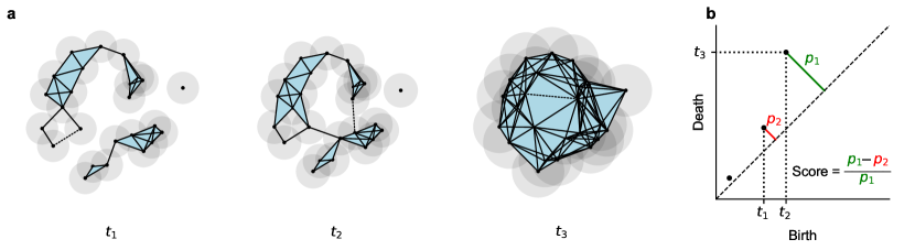
Figure 2: a. Persistent homology applied to a noisy ring ($n=25$) in 2D. Dotted lines show the edges that lead to the birth / death of two loops (Section 3). b. The corresponding persistence diagram with three detected holes. Our hole detection score measures the gap in persistence between the first and the second detected holes (Section 6.1).

Persistent homology computes the homology of a space at different scales. For point clouds, the different scales are often given by growing a ball around each point (Figure 2a), and letting the radius $t$ grow from $0$ to infinity. For each value of $t$, homology groups of the union of all balls are computed to find the holes, and holes that persist for longer time periods $\Delta t$ are considered more prominent. Note that at $t\approx 0$, there are no holes as the balls are non-overlapping, while at sufficiently large $t\gg 0$ there are no holes as all the balls merge together.

To keep the computation tractable, instead of the union of growing balls, persistent homology operates on a so-called filtered simplicial complex (Figure 2a). A simplicial complex is a hypergraph containing points as nodes, edges between nodes, triangles bounded by edges, and so forth. These building blocks are called simplices. At time $t$, the hypergraph encodes all intersections between the balls and suffices to find the holes. The complexes at smaller $t$ values are nested within the complexes at larger $t$ values, and together form a filtered simplicial complex, with $t$ being the filtration parameter (filtration time). In this work, we only use the Vietoris–Rips complex, which includes an $n$-simplex $(v_{0},v_{1},\dots,v_{n})$ at filtration time $t$ if the distance between all pairs $v_{i},v_{j}$ is at most $t$. Therefore, to build a Vietoris–Rips complex, it suffices to provide pairwise distances between all pairs of points. We compute persistent homology via the ripser package (Bauer, 2021).

The output of persistent homology is a set of holes for each dimension (a set of loops, a set of voids, etc.). Each hole has associated birth and death times $(t_{b},t_{d})$, i.e., the first and last filtration value $t$ at which that hole exists. Their difference $p=t_{d}-t_{b}$ is called the persistence or life time of the hole and quantifies its prominence. The birth and death times can be visualized as a scatter plot (Figure 2b), known as the persistence diagram. Points far from the diagonal have high persistence.

This process is illustrated in Figure 2 for a noisy sample of $n=25$ points from a $S^{1}\subset\mathbb{R}^{2}$. At $t_{1}$ a small spurious loop is formed thanks to the inclusion of the dotted edge, but it dies soon afterwards. The ground-truth loop is formed at $t_{2}$ and dies at $t_{3}$, once the hole is completely filled in by triangles. All three loops (one-dimensional holes) found in this dataset are shown in the persistence diagram.

4 The curse of dimensionality for persistence homology

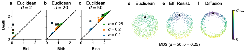
Figure 3: a – c. Persistence diagrams of a noisy ring in different ambient dimensionality and with different amount of noise. d – f. Multidimensional scaling of Euclidean, effective resistance and diffusion distance for a noisy ring in $\mathbb{R}^{50}$. Color indicates the distance to the highlighted point.

While persistent homology has been shown to be robust to small changes in the point positions (Cohen-Steiner et al., 2005), the curse of dimensionality can still severely hurt its performance.

To illustrate, we consider the same toy setting as in Figure 1: we sample points from $S^{1}\subset\mathbb{R}^{d}$, and add Gaussian noise of standard deviation $\sigma$ to each of the ambient coordinates. When $d=2$, higher noise does not affect the birth times but leads to lower death times (Figure 3a), because some points get distorted to the middle of the ring and let the hole fill up at earlier $t$. When we increase the ambient dimensionality to $d=20$, higher noise leads to later birth times (Figure 3b) because the distances are now dominated by the noise dimensions rather than by the ring structure. Finally, for $d=50$ both the birth and the death times increase with $\sigma$ (Figure 3c), such that the ground-truth hole disappears in the cloud of spurious holes.

In other words, in a high-dimensional space, all pairwise distances become similar, and the ring structure fails to stand out. Applying MDS to the Euclidean distance matrix obtained with $d=50$ and $\sigma=0.25$ yields a 2D embedding with almost no visible hole or distance gradient along the ring (Figure 3d). This is a 2D shadow of the fact that the distances due to noise dominate the distances due to the ring structure, making all distances similar. Therefore, the failure modes of persistent homology differ between low- and high-dimensional spaces: While in low dimensions, persistent homology is susceptible to outlier points in the middle of the ring, in high dimensions, there are no points in the middle of the ring; instead, all distances become too similar, hiding the true loops.

5 Background: effective resistance and diffusion distances

Many modern manifold learning and dimensionality reduction methods rely on the $k$-nearest-neighbor ($k$NN) graph of the data. This works well because although distances become increasingly similar in high-dimensional spaces, nearest neighbors still carry information about the data manifold. To make persistence homology overcome high-dimensional noise, we therefore suggest to rely on the $k$NN graph. A natural choice is to use its geodesics, but as we show below this does not work well, likely because a single graph edge across a ring can make the corresponding feature die too early. Instead, we propose to use spectral methods, such as the effective resistance or diffusion distance. Both methods rely on random walks and thus integrate information about all edges.

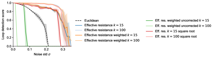
Figure S3: Loop detection score on noisy $S^{1}\subset\mathbb{R}^{50}$ for various versions of effective resistance. There was little difference between using the weighted $k$NN graph, unweighted $k$NN graph, and using the square root of effective resistance based on the unweighted $k$NN graph. The latter got filtered out for high noise levels. Using $k=100$ instead of $k=15$ helped only marginally on this dataset. The uncorrected (naïve) version of effective resistance collapsed at very small noise levels.

For a connected graph $G$ with $n$ nodes, let $A$ be its $n\times n$ adjacency matrix with elements $a_{ij}$. Then the degree matrix $D$ is defined by $D=\text{diag}\{d_{i}\}$, where $d_{i}=\sum_{j=1}^{n}a_{ij}$ are the node degrees. We define $\text{vol}(G)=\sum_{i=1}^{n}d_{i}$. Let $H_{ij}$ be the hitting time from node $i$ to $j$, i.e., the average time it takes a random walker, that starts at node $i$ randomly moving along edges, to reach node $j$. Then the naïve effective resistance is defined as $\tilde{d}^{\text{eff}}_{ij}=(H_{ij}+H_{ji})/\text{vol}(G)$. This naïve version is known to be unsuitable for large graphs (Figure S3) because it mostly depends on the node degrees and reduces to $\tilde{d}^{\text{eff}}_{ij}\approx 1/d_{i}+1/d_{j}$  (von Luxburg et al., 2010a). Therefore we used the corrected version

$$d^{\text{eff}}_{ij}=\tilde{d}^{\text{eff}}_{ij}-\frac{1}{d_{i}}-\frac{1}{d_{j}}+2\frac{a_{ij}}{d_{i}d_{j}}-\frac{a_{ii}}{d_{i}^{2}}-\frac{a_{jj}}{d_{j}^{2}}.$$ (1)

Diffusion distances also rely on random walks. The random walk transition matrix is given by $P=D^{-1}A$. Then $P^{t}_{i,:}$, the $i$-th row of $P^{t}$, holds the probability distribution over nodes after $t$ steps of a random walker starting at node $i$. The diffusion distance is then defined as

$$d_{ij}(t)=\sqrt{\text{vol}(G)}\|(P^{t}_{i,:}-P^{t}_{j,:})D^{-1}\|.$$ (2)

There are many possible random walks between nodes $i$ and $j$ if they both reside in the same densely connected region of the graph, while it is unlikely for a random walker to cross between sparsely connected regions. As a result, both effective resistance and diffusion distance are small between parts of the graph that are densely connected and are robust against single stray edges. Indeed, the MDS embedding of the effective resistance and of the diffusion distance of the ring in ambient $\mathbb{R}^{50}$ both clearly show the ring structure (Figure 3e,f).

6 Spectral distances find holes in high-dimensional spaces

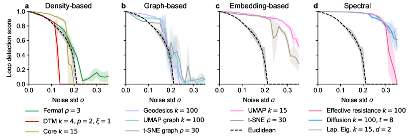
Figure 4: Loop detection score for persistent homology with various distances on a noisy ring in ambient $\mathbb{R}^{50}$. The curves correspond to the best hyperparameters for each distance.

6.1 Benchmark setup

Datasets

In our synthetic benchmark, we evaluated the performance of various distance measures in conjunction with persistent homology on five manifolds: a ring, a pair of linked rings, the eyeglasses dataset (a ring squeezed nearly to a figure eight) (Fernández et al., 2023), the sphere, and the torus. The radii of the rings, the sphere, and the torus’ tube were set to $1$, the bottleneck of the eyeglasses was $0.7$, and the torus’ tube followed a ring of radius $2$. In each case, we uniformly sampled $n=1\,000$ points from the manifold, mapped them isometrically to $\mathbb{R}^{d}$ for $d\in[2,50]$, and then added isotropic Gaussian noise sampled from $\mathcal{N}(\mathbf{0},\sigma^{2}\mathbf{I}_{d})$ for $\sigma\in[0,0.35]$. More details can be found in Appendix D. For each resulting dataset, we computed persistent homology for loops and, for the sphere and the torus, also for voids.

Performance metric

The output of persistent homology is a persistence diagram showing birth and death times for all detected holes. It may be difficult to decide whether this procedure has actually ‘detected’ a hole in the data. Ideally, for a dataset with $m$ ground-truth holes, the persistence diagram should have $m$ points with high persistence while all other points should have low persistence and lie close to the diagonal. Therefore, for $m$ ground-truth features, our metric $s_{m}\in[0,1]$, which we call the hole detection score, is the relative gap between the persistences $p_{m}$ and $p_{m+1}$ of the $m$-th and $(m+1)$-th most persistent features: $s_{m}=(p_{m}-p_{m+1})/p_{m}$. This corresponds to the visual gap between them in the persistence diagram (Figure 2b).

In addition, we set $s_{m}=0$ if all features in the persistence diagram have very low death-to-birth ratios $t_{d}/t_{b}<1.25$. This filters out persistence diagrams with very few detected holes (often only one or two) that die very quickly after being born, which otherwise can sometimes have spuriously high $s_{m}$ values. This was done everywhere apart from the qualitative Figures 1 and 8.

We report the mean over three random seeds. Shading and error bars indicate the standard deviation.

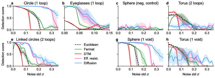
Figure 5: Loop detection score for selected methods on all synthetic datasets in ambient $\mathbb{R}^{50}$. More methods and hyperparameter settings can be found in Figures S4 – S12.

Distance measures

We examined four groups of distances as input to persistent homology, beyond the Euclidean distance. Full definitions are given in Appendix C. The first, density-based group comprises state-of-the-art approaches for persistent homology in presence of noise and outliers. Fermat distances (Fernández et al., 2023) aim to exaggerate large over small distances to gain robustness against outliers. Distance-to-measure (DTM) (Anai et al., 2020) has a similar goal but instead combines the Euclidean distance with the distances from each point to its $k$ nearest neighbors, which are high for low-density outliers. Similarly, the core distance used in the HDBSCAN algorithm (Campello et al., 2015; Damm, 2022) raises each Euclidean distance at least to the distance between incident points and their $k$-th nearest neighbors. The second, graph-based, group consists of distances computed on the $k$NN graph. The geodesic distance on the $k$NN graph was popularized by Isomap (Tenenbaum et al., 2000) and used for persistent homology by Naitzat et al. (2020). Following Gardner et al. (2022) we used distances based on UMAP affinities, and also experimented with the $t$-SNE affinities. In the third, embedding-based, group we computed $t$-SNE and UMAP embeddings and used distances in the 2D embedding space. The final, spectral, group contained distances computed from the $k$NN graph Laplacian (see Section 7): (corrected) effective resistance, diffusion distance, and the distance in the Laplacian Eigenmaps embedding space.

All methods come with hyperparameters. We report the results for the best hyperparameter setting on each dataset. The selected hyperparameter values can be found in Appendix E.

6.2 Benchmark results

On the ring dataset in $\mathbb{R}^{50}$, persistent homology with all distance metrics, including the Euclidean distance, found the correct hole when the noise level $\sigma$ was very low (Figure 4). However, as the amount of noise increased, the performance of Euclidean distance quickly deteriorated, reaching near-zero score at $\sigma\approx 0.25$. Most other distances outperformed the Euclidean distance, at least in the low noise regime. Fermat distance did not have any effect, and neither did DTM distance, which collapsed at $\sigma\approx 0.15$ due to filtering (Figure 4a). Graph-based methods offered only a modest improvement over Euclidean(Figure 4b) as did the core distance. In contrast, embedding-based distances performed very well in this particular case (Figure 4c), but have obvious a priori limitations: for example, a 2D embedding cannot possibly have a void. Finally, all three spectral methods (effective resistance, diffusion, and Laplacian Eigenmaps) showed similarly excellent performance (Figure 4d).

In line with these results, spectral methods outperformed other methods across most synthetic datasets in $\mathbb{R}^{50}$ (Figure 5). DTM collapsed earlier than Euclidean but detected loops on the torus for low noise levels best by a small margin. Fermat distance typically had little effect and provided a benefit over Euclidean only on the eyeglasses and the sphere. Spectral distances outperformed all other methods on all datasets apart from the torus, where effective resistance was on par with Euclidean but diffusion performed poorly. The torus was also the only case where none of the methods achieved loop detection score $s_{m}=1$ in the noiseless $\sigma=0$ regime. On all other datasets diffusion had a small edge over effective resistance for large $\sigma$. Reassuringly, all methods passed the negative control and did not find any persistent loops on the sphere (Figure 5e).

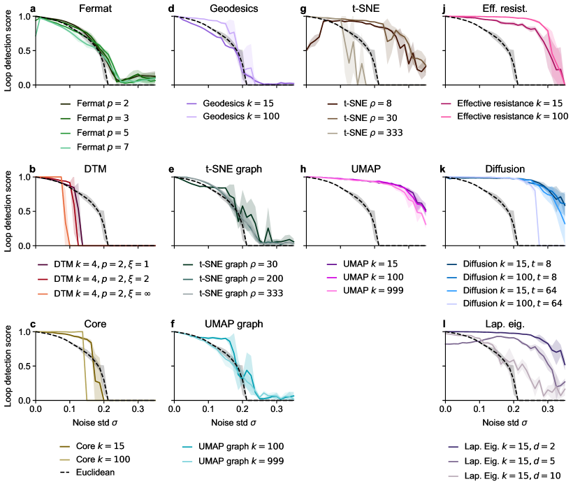
Figure S4: Loop detection score for persistent homology with various distances on a noisy ring in ambient $\mathbb{R}^{50}$. Extension of Figure 4.

As discussed in Section 4, persistent homology with Euclidean distances deteriorates with increasing ambient dimensionality. Using the ring data in $\mathbb{R}^{d}$, we found that if the noise level was fixed at $\sigma=0.25$, no persistent loop was found using Euclidean distances for $d\gtrsim 30$ (Figure 6). In the same setting, DTM deteriorated even more quickly than Euclidean distances. On the other hand, effective resistance and diffusion distance were robust against both the high noise level and the large ambient dimension (Figure 6a, c–e). For details of the effect of the ambient dimension on other methods, compare Figures S4 and S5.

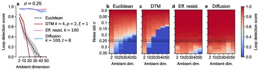
Figure 6: a. Loop detection score of various methods on a noisy ring depending on the ambient dimensionality. Noise $\sigma=0.25$. b – e. Heat maps for $\sigma\in[0,0.35]$ and $d\in[2,50]$.

7 Relation between spectral distances

Laplacian Eigenmaps distance and diffusion distance can be written as Euclidean distances in data representations given by appropriately scaled eigenvectors of the graph Laplacian. In this section we derive a similar closed-form formula for effective resistance.

Using the definitions from Section 5, let $v_{1},\dots,v_{n}$ denote the eigenvectors of the Laplacian $L=D-A$ and $\lambda_{1},\dots,\lambda_{n}$ their eigenvalues. Let further $A^{\text{sym}}=D^{-\frac{1}{2}}AD^{-\frac{1}{2}}$ and $L^{\text{sym}}=I-A^{\text{sym}}$ be the symmetrically normalized adjacency matrix and the symmetrically normalized graph Laplacian. We denote the eigenvectors of $L^{\text{sym}}$ by $u_{1},\dots,u_{n}$ and their eigenvalues by $\mu_{1},\dots,\mu_{n}$ in increasing order. For a connected graph, $\lambda_{1}=\mu_{1}=0$ and $v_{1}=u_{1}=(1,\ldots,1)/\sqrt{n}$.

The $D$-dimensional Laplacian Eigenmaps embedding is given by the first $D$ nontrivial eigenvectors:

$$d_{ij}^{\text{LE}}(D)=\|e_{i}^{\text{LE}}(D)-e_{j}^{\text{LE}}(D)\|,\text{ where }e^{\text{LE}}_{i}(D)=(v_{2,i},\ldots,v_{(D+1),i}).$$ (3)

The diffusion distance for $t$ diffusion steps is given by (Coifman & Lafon, 2006)

$$d_{ij}^{\text{diff}}(t)=\|e_{i}^{\text{diff}}(t)-e_{j}^{\text{diff}}(t)\|,\text{ where }e_{i}^{\text{diff}}(t)=\frac{1}{\sqrt{d_{i}}}\left((1-\mu_{2})^{t}u_{2,i},\ldots,(1-\mu_{n})^{t}u_{n,i}\right).$$ (4)

Finally, the original uncorrected version of effective resistance is given by (Fouss et al., 2007)

$$\tilde{d}^{\text{eff}}_{ij}=\|\tilde{e}_{i}^{\text{eff}}-\tilde{e}_{j}^{\text{eff}}\|^{2},\text{ where }\tilde{e}_{i}^{\text{eff}}=\left(\frac{1}{\sqrt{\lambda_{2}}}v_{2,i},\ldots,\frac{1}{\sqrt{\lambda_{n}}}v_{n,i}\right).$$ (5)

Here we show that the corrected effective resistance (von Luxburg et al., 2010a) can also be written in this form (see the proof in Appendix A):

Proposition 1.

The corrected effective resistance distance can be computed by

$$d_{ij}^{\textnormal{eff}}=\|e_{i}^{\textnormal{eff}}-e_{j}^{\textnormal{eff}}\|^{2},\text{ where }e_{i}^{\textnormal{eff}}=\frac{1}{\sqrt{d_{i}}}\left(\frac{1-\mu_{2}}{\sqrt{\mu_{2}}}u_{2,i},\ldots,\frac{1-\mu_{n}}{\sqrt{\mu_{n}}}u_{n,i}\right).$$ (6)

As we operate on the symmetric $k$NN graph ($\text{s}k\text{NN}$), which contains edge $ij$ if $i$ is among the $k$ nearest neighbors of $j$ or vice versa, the degree distribution is close to constant. As a result, the $1/\sqrt{d_{i}}$ terms have little effect and the eigenvectors and the relative size of the eigenvalues do not depend much on the normalization of the Laplacian. Note that effective resistance is a squared Euclidean distance. However, omitting the square amounts to taking the square root of all birth and death times, maintaining the loop detection performance of effective resistance (Figure S3). Therefore, the main difference between the spectral methods boils down to how they decay higher eigenvectors based on the corresponding eigenvalues.

The naïve effective resistance decays the eigenvectors with $1/\sqrt{\lambda_{i}}$, which is much slower than diffusion distances’ $(1-\mu_{i})^{t}$ for ($t\in[8,64]$), while corrected effective resistance shows intermediate behaviour (Figure 7b). The correction matters little for the $S^{1}\subset\mathbb{R}^{50}$ in the absence of noise, when the first eigenvalues are much smaller than the rest and dominate the embedding (Figure 7a,c) but becomes important as the noise and consequently the low eigenvalues increase (Figure 7a,d,e). As the noise increases, the decay for diffusion distances gets closer to a step function preserving only the first two non-constant eigenvectors, similar to Laplacian Eigenmaps with $D=2$ (Figure 7c–e).

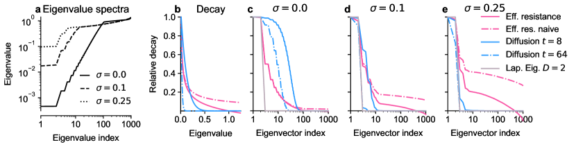
Figure 7: a. Eigenvalue spectra of the $\text{s}k\text{NN}$ graph Laplacian for the noisy ring in ambient $\mathbb{R}^{50}$ for noise levels $\sigma=\{0.0,0.1,0.25\}$. b. Decay of eigenvector contribution based on the eigenvalue for effective resistance and diffusion distances. c – e. Relative contribution of each eigenvector for effective resistance, diffusion distance and Laplacian Eigenmaps for various noise levels (Section 7).

8 Detecting cycles in single-cell RNA-sequencing data

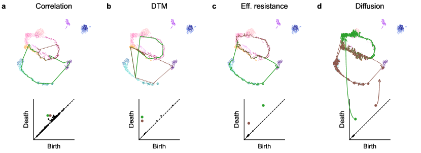
Figure 8: Malaria dataset. a – d. Representatives of the two most persistent loops overlaid on UMAP embedding (top) and persistence diagrams (bottom) using four methods. Biology dictates that there should be two loops (in warm colors and in cold colors) connected as in a figure eight.

We applied our methods to six single-cell RNA-sequencing datasets: Malaria (Howick et al., 2019), Neurosphere, and Hippocampus from (Zheng et al., 2022), HeLa2 (Schwabe et al., 2020), Neural IPCs (Braun et al., 2022), and Pancreas (Bastidas-Ponce et al., 2019). Single-cell RNA-sequencing data consists of expression levels for thousands of genes in individual cells, so the data is high-dimensional and notoriously noisy. All selected datasets are known to contain ring structures, usually corresponding to the cell division cycle. In each case, we followed existing preprocessing pipelines leading to representations with $10$ to $5\,156$ dimensions. Datasets with more than $4\,000$ cells were downsampled to $n=1\,000$ (Appendix D).

The Malaria dataset is expected to contain two cycles: the parasite replication cycle in red blood cells, and the parasite transmission cycle between human and mosquito hosts. Following Howick et al. (2019), we based all computations for this dataset (and all derived distances) on the correlation distance instead of the Euclidean distance. Persistent homology based on the correlation distance itself failed to correctly identify the two ground-truth cycles and DTM produced only rough approximations (Figure 8a,b). But both effective resistance and diffusion distance successfully uncovered both cycles, with $s_{2}>0.9$ (Figure 8 c,d).

Across all six datasets, the detection scores were higher for spectral methods than for their competitors (Figure 9). Furthermore, we manually investigated representative loops for all considered methods on all datasets and found several cases where the most persistent loop(s) was/were likely not correct (hatched bars in Figure 9). Overall, we found that the spectral methods, and in particular effective resistance, could reliably find the correct loops with high detection score. Persistent homology based on the $t$-SNE and UMAP embeddings could also often identify the correct loop structure and on average worked better than vanilla persistent homology, Fermat distances, and DTM.

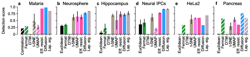
Figure 9: Loop detection scores on six high-dimensional scRNA-seq datasets. Hatched bars indicate implausible representatives. See Figure S13 for detection scores for different hyperparameter values.

9 Discussion

In this work we asked how to use persistent homology on high-dimensional noisy datasets. We demonstrated that, as the dimensionality of the data increases, the main problem for persistent homology shifts from handling outliers to handling noise dimensions (Section 4). We used a synthetic benchmark to show that vanilla persistent homology and many of its existing extensions struggle to find the correct topology in this setting, whereas spectral methods based on the $k$NN graph, such as the effective resistance and diffusion distances, work well (Section 6). We derived an expression for effective resistance based on the eigendecomposition of the $k$NN graph Laplacian, relating it to diffusion distances and to Laplacian Eigenmaps (Section 7). Finally, we showed that spectral distances outperform all competitors on real-world single-cell data (Section 8).

In the real-world applications, it was important to look at representatives of detected holes as sometimes methods found persistent, but arguably incorrect loops. That said, each hole homology class has many different representative cycles, making interpretation difficult. Given ground-truth cycles, an automatic procedure for evaluating cycle correctness remains an interesting research question.

Dimensionality reduction methods are designed to handle high-dimensional data. In the case of $t$-SNE and UMAP, we observed that persistent homology based on the 2D embeddings performed much better than using their $\text{s}k\text{NN}$ graph affinities, underlining that the key to the success of these methods is in their embedding optimization rather than their notion of similarity (Böhm et al., 2022; Damrich & Hamprecht, 2021). In contrast, spectral distances on the $\text{s}k\text{NN}$ graph worked well without a low-dimensional embedding (Sections 6, 8).

One limitation of persistent homology is its computational complexity. It scales as $\mathcal{O}(n^{3(\delta+1)})$ for $n$ points and topological holes of dimension $\delta$, and has high memory consumption. This aggravates other problems of high-dimensional datasets as dense sampling in high-dimensional space would require a prohibitively large sample size. Subsampling techniques as proposed in Chazal et al. (2015) are one possible solution. When combining persistent homology with non-Euclidean distance measures, the approach of Bendich et al. (2011), who performed the subsampling after computation of the distance matrix, is particularly attractive, and forms an interesting avenue for future research.

Acknowledgments

We thank Enrique Fita Sanmartin and Ulrike von Luxburg for productive discussions on effective resistance and persistent homology, and Benjamin Dunn, Erik Hermansen, and David Klindt for helpful discussions on combining persistent homology with other dissimilarities than Euclidean distance. Moreover, we thank Sten Linnarsson and Miri Danan Gotthold for sharing the scVI representation of their pallium data.

Reproducibility statement

We prove our theoretical statements in Appendices A and B. We describe the methods and datasets used in detail in Appendices C and D. The hyperparameters for the reported results can be found in Appendix E. Finally, we give details on our implementation and hardware in Appendix F. Our code is available at https://github.com/berenslab/eff-ph/tree/arxiv-v1, which also includes the Neural IPC data. To obtain the other datasets, see Appendix D.

Supplementary text

Appendix A Effective resistance as spectral method

Let $G$ be a weighted, connected graph of $n$ nodes. Denote by $A=(a_{ij})_{i,j=1,\dots,n}$ the weighted adjacency matrix and by $D=\text{diag}(d_{i})$ the degree matrix, where $d_{i}=\sum_{j=1,\dots,n}a_{ij}$ are the degrees. We define $\text{vol}(G)=\sum_{i}d_{i}$. Let further $A^{\text{sym}}=D^{-\frac{1}{2}}AD^{-\frac{1}{2}}$ and $L^{\text{sym}}=I-A^{\text{sym}}$ be the symmetrically normalized adjacency matrix and the symmetrically normalized graph Laplacian. Denote the eigenvectors of $L^{\text{sym}}$ by $u_{1},\dots,u_{n}$ and their eigenvalues by $\mu_{1},\dots,\mu_{n}$ in increasing order. The eigenvectors and eigenvalues of $A^{\text{sym}}$ are $u_{1},\dots,u_{n}$ and $1-\mu_{1},\dots,1-\mu_{n}$.

Definition 2.

The effective resistance distance between nodes $i$ and $j$ is defined as

$$\tilde{d}^{\text{eff}}_{ij}=\frac{1}{\text{vol}(G)}(H_{ij}+H_{ji}),$$ (7)

where $H_{ij}$ is the hitting time from $i$ to $j$, i.e., the expected number of steps that a random walker starting at node $i$ takes to reach node $j$ for the first time.
The corrected effective resistance distance between nodes $i$ and $j$ is defined as

$$d^{\text{eff}}_{ij}=\tilde{d}^{\text{eff}}_{ij}-\frac{1}{d_{i}}-\frac{1}{d_{j}}+2\frac{a_{ij}}{d_{i}d_{j}}-\frac{a_{ii}}{d_{i}^{2}}-\frac{a_{jj}}{d_{j}^{2}}.$$ (8)

The following proposition is an elaboration of Prop. 4 in von Luxburg et al. (2010a).

Proposition 3.

The corrected effective resistance distance $d^{\text{eff}}_{ij}$ between nodes $i$ and $j$ can be computed by $d^{\text{eff}}_{ij}=\|e_{i}-e_{j}\|^{2}$, where

$$e_{i}=\frac{1}{\sqrt{d_{i}}}\left(\frac{1-\mu_{2}}{\sqrt{\mu_{2}}}u_{2,i},\dots,\frac{1-\mu_{n}}{\sqrt{\mu_{n}}}u_{n,i}\right).$$

Proof.

By the fourth step of the large equation in the proof of Proposition 2 in von Luxburg et al. (2010b), we have

$$\frac{1}{\text{vol}(G)}H_{ij}=\frac{1}{d_{j}}+\langle b_{j},A^{\text{sym}}(b_{j}-b_{i})\rangle+\sum_{r=2}^{n}\frac{1}{\mu_{r}}\langle A^{\text{sym}}b_{j},u_{r}(u_{r})^{T}(A^{\text{sym}}(b_{j}-b_{i}))\rangle,$$ (9)

where $b_{i}=\frac{1}{\sqrt{d_{i}}}e_{i}=D^{-\frac{1}{2}}e_{i}$ with $e_{i}$ the $i$-th standard basis vector.
Adding this expression for $ij$ and $ji$ and using the definition of $\tilde{d}^{\text{eff}}_{ij}$, we get

$$\tilde{d}^{\text{eff}}_{ij}-\frac{1}{d_{i}}-\frac{1}{d_{j}} =\frac{1}{\text{vol}(G)}(H_{ij}+H_{ji})-\frac{1}{d_{i}}-\frac{1}{d_{j}}$$ (10)

$$=\langle b_{j},A^{\text{sym}}(b_{j}-b_{i})\rangle+\langle b_{i},A^{\text{sym}}(b_{i}-b_{j})\rangle$$ (11)

$$\quad+\sum_{r=2}^{n}\frac{1}{\mu_{r}}\langle A^{\text{sym}}b_{j},u_{r}(u_{r})^{T}(A^{\text{sym}}(b_{j}-b_{i}))\rangle$$ (12)

$$\quad+\sum_{r=2}^{n}\frac{1}{\mu_{r}}\langle A^{\text{sym}}b_{i},u_{r}(u_{r})^{T}(A^{\text{sym}}(b_{i}-b_{j}))\rangle$$ (13)

$$=\langle b_{j}-b_{i},A^{\text{sym}}(b_{j}-b_{i})\rangle$$ (14)

$$\quad+\sum_{r=2}^{n}\frac{1}{\mu_{r}}\langle A^{\text{sym}}(b_{j}-b_{i}),u_{r}(u_{r})^{T}(A^{\text{sym}}(b_{j}-b_{i}))\rangle$$ (15)

For ease of exposition, we treat both summands separately. By unpacking the definitions and symmerty of $D$, we get

$$\langle b_{j}-b_{i},A^{\text{sym}}(b_{j}-b_{i})\rangle =\langle D^{-\frac{1}{2}}(e_{j}-e_{i}),A^{\text{sym}}D^{-\frac{1}{2}}(e_{j}-e_{i})\rangle$$ (16)

$$=\langle(e_{j}-e_{i}),D^{-1}AD^{-1}(e_{j}-e_{i})\rangle$$ (17)

$$=\frac{a_{jj}}{d_{j}^{2}}-2\frac{a_{ij}}{d_{i}d_{j}}+\frac{a_{ii}}{d_{i}^{2}}$$ (18)

Since the $u_{r}$ are eigenvectors of $A^{\text{sym}}$ with eigenvalue $1-\mu_{r}$ and $A^{\text{sym}}$ is symmetric, we also get

$$\sum_{r=2}^{n}\frac{1}{\mu_{r}}\langle A^{\text{sym}}(b_{j}-b_{i}),u_{r}(u_{r})^{T}(A^{\text{sym}}(b_{j}-b_{i}))\rangle$$ (19)

$$= \sum_{r=2}^{n}\frac{1}{\mu_{r}}\langle(b_{j}-b_{i}),(A^{\text{sym}}u_{r})(A^{\text{sym}}u_{r})^{T}(b_{j}-b_{i}))\rangle$$ (20)

$$= \sum_{r=2}^{n}\frac{1}{\mu_{r}}\langle(b_{j}-b_{i}),(1-\mu_{r})u_{r}((1-\mu_{r})u_{r})^{T}(b_{j}-b_{i}))\rangle$$ (21)

$$= \sum_{r=2}^{n}\left(\frac{1-\mu_{r}}{\sqrt{\mu_{r}}}u_{r}^{T}D^{-\frac{1}{2}}(e_{j}-e_{i})\right)^{2}$$ (22)

$$= \left\|\frac{1}{\sqrt{d_{j}}}\left(\frac{1-\mu_{r}}{\sqrt{\mu_{r}}}u_{r,j}\right)_{r=2,\dots,n}-\frac{1}{\sqrt{d_{i}}}\left(\frac{1-\mu_{r}}{\sqrt{\mu_{r}}}u_{r,i}\right)_{r=2,\dots,n}\right\|^{2}$$ (23)

$$= \|e_{j}-e_{i}\|^{2}$$ (24)

Putting everything together yields the result

$$d^{\text{eff}}_{ij} =\tilde{d}^{\text{eff}}_{ij}-\frac{1}{d_{i}}-\frac{1}{d_{j}}+2\frac{a_{ij}}{d_{i}d_{j}}-\frac{a_{ii}}{d_{i}^{2}}-\frac{a_{jj}}{d_{j}^{2}}$$ (25)

$$=\frac{a_{jj}}{d_{j}^{2}}-2\frac{a_{ij}}{d_{i}d_{j}}+\frac{a_{ii}}{d_{i}^{2}}+\|e_{j}-e_{i}\|^{2}+2\frac{a_{ij}}{d_{i}d_{j}}-\frac{a_{ii}}{d_{i}^{2}}-\frac{a_{jj}}{d_{j}^{2}}$$ (26)

$$=\|e_{j}-e_{i}\|^{2}.$$ (27)

∎

Appendix B Pairwise noise distances in high-dimensional spaces

Consider two independent random variables $X$ and $Y$, both following a $d$-dimensional spherical normal distribution: $X,Y\sim\mathcal{N}(\mathbf{0},\sigma^{2}\mathbf{I}_{d})$. Their difference $X-Y$ is also normally distributed $X-Y\sim\mathcal{N}(\mathbf{0},2\sigma^{2}\mathbf{I}_{d})$, so the expected squared distance is simply $\mathbb{E}(\|X-Y\|^{2})=2\sigma^{2}d$.

However, persistent homology operates on non-squared distances, which is why we are interested in $\mathbb{E}(\|X-Y\|)$. Using a somewhat more involved calculation, it can be shown that it scales as $\sqrt{2}\sigma d$.

Proposition 4.

Let $X$ and $Y$ be isotropic $d$-dimensional normally distributed random variables, $X,Y\sim\mathcal{N}(\mathbf{0},\sigma^{2}\mathbf{I}_{d})$, where $\mathbf{I}_{d}$ is the $d$-dimensional identity matrix and $\sigma>0$. Then the expected distance between $X$ and $Y$ is

$$\mathbb{E}(\|X-Y\|)=2\sigma\frac{\Gamma(\frac{d+1}{2})}{\Gamma(\frac{d}{2})}=2\sigma\left(\sqrt{\frac{d}{2}}+O(d^{-0.5})\right).$$ (28)

Proof.

The random variable $X-Y$ is also normally distributed, $X-Y\sim\mathcal{N}(\mathbf{0},2\sigma^{2}\mathbf{I}_{d})$. Therefore, $\frac{\|X-Y\|}{\sqrt{2}\sigma}$ is Chi-distributed, with mean $\sqrt{2}\frac{\Gamma(\frac{d+1}{2})}{\Gamma(\frac{d}{2})}$. This shows the first part of the claim.

For the approximate expression, we only treat the case of even $d$ for ease of exposition. Let $d=2d^{\prime}$. Then by properties of the Gamma function and the binomial coefficient, we have

$$\frac{\Gamma(\frac{d+1}{2})}{\Gamma(\frac{d}{2})} =\frac{\Gamma(d^{\prime}+0.5)}{\Gamma(d^{\prime})}=\frac{\sqrt{\pi}\frac{(2d^{\prime}-1)!!}{2^{d^{\prime}}}}{(d^{\prime}-1)!}=\sqrt{\pi}\frac{\frac{(2d^{\prime})!}{4^{d^{\prime}}d^{\prime}!}}{(d^{\prime}-1)!}=\sqrt{\pi}d^{\prime}4^{-d^{\prime}}\binom{2d^{\prime}}{d^{\prime}}$$ (29)

$$\approx\sqrt{\pi}d^{\prime}4^{-d^{\prime}}\left(\frac{4^{d^{\prime}}}{\sqrt{\pi d^{\prime}}}+4^{d^{\prime}}O(d^{\prime-1.5})\right)=\sqrt{d^{\prime}}+O(d^{\prime-0.5})=\sqrt{\frac{d}{2}}+O(d^{-0.5}),$$ (30)

where the approximation of the central binomial coefficient holds asymptotically (Luke, 1969, p. 35). ∎

Appendix C Details on the distances

Let $x_{1},\dots,x_{n}\in\mathbb{R}^{d}$. We denote pairwise Euclidean distances by $d_{ij}=\|x_{i}-x_{j}\|$, the $k$ nearest neighbors of $x_{i}$ by $x_{i_{1}},\dots,x_{i_{k}}$, and the set containing them by $N_{i}$. Many distances rely on the symmetric $k$-nearest-neighbor ($\text{s}k\text{NN}$) graph. This graph contains edge $ij$ if $x_{i}$ is among the $k$ nearest neighbors of $x_{j}$ or vice versa.

Fermat distances

For $p\geq 1$, the Fermat distance is defined as

$$d_{ij}^{F}(p)=\inf_{\pi}\bigg{(}\sum_{(uv)\in\pi}d_{uv}^{p}\bigg{)},$$ (31)

where the infimum is taken over all finite paths from $x_{i}$ to $x_{j}$ in the complete graph with edge weights $d_{ij}^{p}$. As a speed-up, Fernández et al. (2023) suggested to compute the shortest paths only on the $k$NN graph, but for our sample sizes we could perform the calculation on the complete graph. For $p=1$ this reduces to normal Euclidean distances due to the triangle inequality. We used $p\in\{2,3,5,7\}$.

DTM distances

The DTM distances depend on three hyperparameters: the number of nearest neighbors $k$, one hyperparameter controlling the distance to measure $p$, and finally a hyperparameter $\xi$ controlling the combination of DTM and Euclidean distance. The DTM value for each point is given by

$$\text{dtm}_{i}=\begin{cases}\sqrt[p]{\sum_{\kappa=1}^{k}\|x_{i}-x_{i_{\kappa}}\|^{p}/k}&\text{ if }p<\infty\\ \|x_{i}-x_{i_{k}}\|&\text{ else}.\end{cases}$$ (32)

These values are combined with pairwise Euclidean distances to give pairwise DTM distances:

$$d^{\text{DTM}}_{ij}(k,p,\xi)=\begin{cases}\max(\text{dtm}_{i},\text{dtm}_{j})&\text{ if }\|x_{i}-x_{j}\|\leq\sqrt[\xi]{|\text{dtm}_{i}^{\xi}-\text{dtm}_{j}^{\xi}|}\\ t&\text{ else},\end{cases}$$ (33)

where $t$ is the only positive root of $\sqrt[\xi]{t^{\xi}-\text{dtm}_{i}^{\xi}}+\sqrt[\xi]{t^{\xi}-\text{dtm}_{j}^{\xi}}=d_{ij}$. We only considered the values $\xi\in\{1,2,\infty\}$, for which the there are closed-form solutions:

$$t=\begin{cases}(\text{dtm}_{i}+\text{dtm}_{j}+d_{ij})/2&\text{ if }\xi=1\\ \sqrt{((\text{dtm}_{i}+\text{dtm}_{j})^{2}+d_{ij}^{2})\cdot((\text{dtm}_{i}-\text{dtm}_{j})^{2}+d_{ij}^{2})}/(2d_{ij})&\text{ if }\xi=2\\ \max(\text{dtm}_{i},\text{dtm}_{j},d_{ij}/2)&\text{ if }\xi=\infty.\end{cases}$$ (34)

We used $k\in\{4,15,100\}$, $p\in\{2,\infty\}$, and $\xi\in\{1,2,\infty\}$.

Core distance

The core distance is similar to the DTM distance with $\xi=\infty$ and $p=\infty$ and is given by

$$d^{\text{core}}_{ij}(k)=\max(d_{ij},\|x_{i}-x_{i_{k}}\|,\|x_{j}-x_{j_{k}}\|).$$ (35)

We used $k\in\{15,100\}$.

$t$-SNE graph affinities

The $t$-SNE affinities are given by

$$p_{ij}=\frac{p_{i|j}+p_{j|i}}{2n},\quad p_{j|i}=\frac{\nu_{j|i}}{\sum_{k\neq i}\nu_{k|i}},\quad\nu_{j|i}=\begin{cases}\exp\left(\|x_{i}-x_{j}\|^{2}/(2\sigma_{i}^{2})\right)&\text{ if }x_{j}\in N_{i}\\ 0&\text{ else,}\end{cases}$$ (36)

where $\sigma_{i}$ is selected such that the distribution $p_{j|i}$ has pre-specified perplexity $\rho$. Standard implementations of $t$-SNE use $k=3\rho$. We transformed $t$-SNE affinities into pairwise distances by taking the negative logarithm. Pairs $x_{i}$ and $x_{j}$ with $p_{ij}=0$ (i.e. not in the $k$NN graph) get distance $\infty$. We used $\rho\in\{30,200,333\}$.

UMAP graph affinities

The UMAP affinities are given by

$$\mu_{ij}=\mu_{i|j}+\mu_{j|i}-\mu_{i|j}\mu_{j|i},\quad\mu_{j|i}=\begin{cases}\exp\big{(}-(d_{ij}-\mu_{i})/\sigma_{i}\big{)}&\text{ for }j\in\{i_{1},\dots,i_{k}\}\\ 0&\text{ else,}\end{cases}$$ (37)

where $\mu_{i}=\|x_{i}-x_{i_{1}}\|$ is the distance between $x_{i}$ and its nearest non-identical neighbor. The scale parameter $\sigma_{i}$ is selected such that

$$\sum_{\kappa=1}^{k}\exp\Big{(}-\big{(}d(x_{i},x_{i_{\kappa}})-\mu_{i}\big{)}/\sigma_{i}\Big{)}=\log_{2}(k).$$ (38)

As above, to convert these affinities into distances, we take the negative logarithm and handle zero similarities as for the $t$-SNE case. We used $k\in\{100,999\}$; $k=15$ resulted in memory overflow on one of the void-containing datasets.

Gardner et al. (2022) and Hermansen et al. (2022) first used these distances, but omitted $\mu_{i}$, which we included to completely reproduce UMAP’s affinities.

Note that distances derived from UMAP and $t$-SNE affinities are not guaranteed to obey the triangle inequality.

Geodesic distances

We computed the shortest path distances between all pairs of nodes in the $\text{s}k\text{NN}$ graph with edges weighted by their Euclidean distances. We used the python function scipy.sparse.csgraph.shortest_path. We used $k=\{15,100\}$.

UMAP embedding

We computed the UMAP embeddings in $2$ embedding dimensions using $750$ optimization epochs, min_dist of $0.1$, exactly computed $k$ nearest neighbors, and PCA initialization. Then we used Euclidean distances between the embedding points. We used UMAP commit a7606f2. We used $k\in\{15,100,999\}$.

$t$-SNE embedding

We computed the $t$-SNE embeddings in $2$ embedding dimensions using openTSNE (Poličar et al., 2019) with default parameters, but providing manually computed affinities. For that we used standard Gaussian affinities on the $\text{s}k\text{NN}$ graph with $k=3\rho$. Then we used the Euclidean distances between the embedding points. We used perplexity $\rho\in\{8,30,333\}$.

For UMAP and $t$-SNE affinities as well as for UMAP and $t$-SNE embeddings we computed the $\text{s}k\text{NN}$ graph with PyKeOps (Charlier et al., 2021) instead of using the default approximate methods. The UMAP and $t$-SNE affinities (without negative logarithm) were used by the corresponding embedding methods.

Effective resistance

We computed the effective resistance on the $\text{s}k\text{NN}$graph. Following the analogy with resistances in an electric circuit, if the $\text{s}k\text{NN}$ graph is disconnected, we computed the effective resistance separately in each connected component and set resistances between components to $\infty$. The uncorrected resistances were computed via the pseudoinverse of the graph Laplacian

$$\tilde{d}^{\text{eff}}_{ij}=l_{ii}^{\dagger}-2l_{ij}^{\dagger}+l_{jj}^{\dagger},$$ (39)

where $l_{ij}^{\dagger}$ is the $ij$-th entry of the pseudoinverse of the non-normalized $\text{s}k\text{NN}$ graph Laplacian. For the corrected version, we used

$$d^{\text{eff}}_{ij}=\tilde{d}^{\text{eff}}_{ij}-\frac{1}{d_{i}}-\frac{1}{d_{j}}+2\frac{a_{ij}}{d_{i}d_{j}}-\frac{a_{ii}}{d_{i}^{2}}-\frac{a_{jj}}{d_{j}^{2}}.$$ (40)

For the weighted version of effective resistance, each edge in the $\text{s}k\text{NN}$ graph was weighted by the inverse of the Euclidean distance. We experimented with the weighted and unweighted versions, but only reported the unweighted version in the paper (as the difference was always minor). We also experimented with the unweighted and uncorrected version and saw that correcting is crucial for high noise levels (Figure S3). We used $k~{}\in\{15,100\}$.

Diffusion distance

We computed the diffusion distances on the unweighted $\text{s}k\text{NN}$ graph directly by equation (2), i.e.,

$$d_{ij}(t)=\sqrt{\text{vol}(G)}\|(P^{t}_{i,:}-P^{t}_{j,:})D^{-1}\|.$$ (41)

Note that our $\text{s}k\text{NN}$ graphs do not contain self-loops. We used $k\in\{15,100\}$ and $t\in\{8,64\}$.

Laplacian Eigenmaps

For a dataset with $K$ connected components, we computed the $K+D$ eigenvectors $v_{1},\dots,v_{K+D}$ of the un-normalized graph Laplacian of the $\text{s}k\text{NN}$ graph and discarded the first $K$ eigenvectors $v_{1},\dots,v_{K}$, which are just indicators for the connected components. Then we computed the Euclidean distances between the embedding vectors $e^{\text{LE}}_{i}=(v_{K+1,i},\ldots,v_{(K+D),i})$. We used $k=15$ and $D\in\{2,5,10\}$. Alternatively, one can compute Laplacian Eigenmaps using the normalized graph Laplacian $L^{\text{sym}}=D^{-\frac{1}{2}}LD^{-\frac{1}{2}}$. We tried this for $D=2$ but obtained very similar embeddings.

For all methods, we replaced infinite distances with twice the maximal finite distance to be able to compute our hole detection scores.

Appendix D Datasets

D.1 Synthetic datasets

The synthetic, noiseless datasets with $n=1\,000$ points each are depicted in Figure S1.

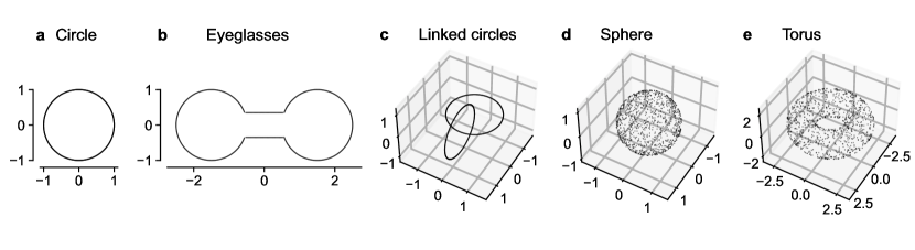
Figure S1: Synthetic, noiseless datasets with $n=1\,000$ points each.

Circle

The circle dataset consists of $n$ points equidistantly spaced along a circle of radius $r=1$.

Linked circles

The linked circles dataset consists of two circle datasets of $n/2$ points each, arranged such that each circle perpendicularly intersects the plane spanned by the other.

Eyeglasses

The eyeglasses dataset consists of four parts: Two ring segments of arclength $\pi+2.4$ and radius $r=1$, centered $3$ units apart with the gaps facing each other. The third and fourth part are two straight line segments of length $0.53$, separated by $0.7$ units linking up the two ring segments. The circle segments consist of $0.425n$ equidistantly distributed points each and the line segments consist of $0.075n$ equispaced points each. As the length scale of this dataset is dominated by the bottleneck between the two line segments, we only considered noise levels $\sigma\in[0,0.15]$ for this dataset, as at this point the bottleneck essentially merges in $\mathbb{R}^{2}$.

Sphere

The sphere dataset consists of $n$ points sampled uniformly from a sphere $S^{2}$ with radius $r=1$.

Torus

The torus dataset consists of $n$ points sampled uniformly from a torus. The radius of the torus’ tube was $r=1$ and the radius of the center of the tube was $R=2$. Note that we do not sample the points to have uniform angle distribution along the tube’s and the tube center’s circle, but uniform on the surface of the torus.

High-dimensional noise

we mapped each dataset to $\mathbb{R}^{d}$ for $d\in[2,50]$ using a random matrix $\mathbf{V}$ of size $d\times 2$ or $d\times 3$ with orthonormal columns, and then added isotropic Gaussian noise sampled from $\mathcal{N}(\mathbf{0},\sigma^{2}\mathbf{I}_{d})$ for $\sigma\in[0,0.35]$. The orthogonal embedding in $\mathbb{R}^{d}$ does not change the shape of the data. The procedure is equivalent to adding $d-2$ or $d-3$ zero dimensions and then randomly rotating the resulting dataset in $\mathbb{R}^{d}$.

D.2 Single-cell datasets

We depict 2D embeddings of all single-cell datasets in Figure S2.

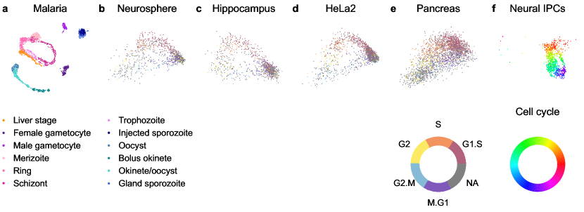
Figure S2: 2D embeddings of all six single-cell datasets. a, f. UMAP embeddings of the Malaria (Howick et al., 2019) and the Neural IPC datasets (Braun et al., 2022). We recomputed the embedding for the Malaria dataset using UMAP hyperparameters provided in the original publication, and subsetted a provided UMAP of a superset of telencephalic exitatory cells to the Neural IPC. Text legend refers to Malaria cell types. b – e. 2D linear projection constructed to bring out the cell cycle (‘tricycle embedding’) (Zheng et al., 2022) of the Neurosphere, Hippocampus, HeLa2, and Pancreas datasets. We used the projection coordinates provided by Zheng et al. (2022).

Malaria

The Malaria dataset (Howick et al., 2019) consists of gene expression measurement of $5\,126$ genes obtained with the modified SmartSeq2 approach of Reid et al. (2018) in $n=1\,787$ cells from the entire life cycle of Plasmodium berghei. The resulting transcripts were pre-processed with the trimmed mean of M-values method (Robinson & Oshlack, 2010). We obtained the pre-processed data from https://github.com/vhowick/MalariaCellAtlas/raw/v1.0/Expression_Matrices/Smartseq2/SS2_tmmlogcounts.csv.zip. The UMAP embedding shown in Figure 8 follows the authors’ setup and uses correlation distance as input metric, $k=10$ nearest neighbors, and a min_dist of $1$ and spread of $2$. Note that when computing persistent homology with UMAP-related distances, we used our normal UMAP hyperparameters and never changed min_dist or spread.

Neural IPCs

The Neural IPC dataset (Braun et al., 2022) consists of gene expressions of $n=26\,625$ neural IPCs from the developing human cortex. scVI (Lopez et al., 2018) was used to integrate cells with different ages and donors based on the $700$ most highly variable genes, resulting in a $d=10$ dimensional embedding. Braun et al. (2022) shared this representation with us for a superset of $297\,927$ telencephalic exitatory cells. We limited our analysis to the neural IPCs because they formed a particularly prominent cell cycle. The data can be downloaded from https://github.com/berenslab/eff-ph/blob/main/data/pallium_scVI_IPC/pallium_scVI_IPC.h5.

Neurosphere

The Neurosphere dataset (Zheng et al., 2022) consists of gene expressions for $n=12\,805$ cells from the mouse neurosphere. After quality control, the data was library size normalized and $\log_{2}$ transformed. Seurat was used to integrate different samples based on the first $30$ PCs of the top $2\,000$ highly variable genes, resulting in a $12\,805\times 2\,000$ matrix of $\log_{2}$ transformed expressions.These were subsetted to the genes in the gene ontology (GO) term cell cycle (GO:0007049). The $500$ most highly variable genes are selected and a PCA was computed to $d=20$. The GO PCA representation was downloaded from https://zenodo.org/record/5519841/files/neurosphere.qs.

Hippocampus

The Hippocampus dataset (Zheng et al., 2022) consists of gene expressions for $n=9\,188$ mouse hippocampal NPCs. The pre-processing was the same as for the Neurosphere dataset. The GO PCA representation was downloaded from https://zenodo.org/record/5519841/files/hipp.qs.

HeLa2

The HeLa2 dataset (Schwabe et al., 2020; Zheng et al., 2022) consists of gene expressions for $2\,463$ cells from a human cell line derived from cervical cancer. After quality control, the data was library size normalized and $\log_{2}$ transformed. From here the GO PCA computation was the same as for the neurosphere dataset. The GO PCA representation was downloaded from https://zenodo.org/record/5519841/files/HeLa2.qs.

Pancreas

The Pancreas dataset (Bastidas-Ponce et al., 2019; Zheng et al., 2022) consists of gene expressions for $3\,559$ cells from the mouse endocrine pancreas. After quality control, the data was library size normalized and $\log_{2}$ transformed. From here the GO PCA computation was the same as for the neurosphere dataset. The GO PCA representation was downloaded from https://zenodo.org/record/5519841/files/endo.qs.

Appendix E Hyperparameter selection

For each of the datasets and hole dimensions, we showed the result with the best hyperparameter setting. For the synthetic experiments, this meant the highest area under the hole detection score curve, while for the single-cell datasets it meant the highest loop detection score. Here, we give details of the selected hyperparamters.

For Figure 1 we used effective resistance with $k=100$ as in Figure 4.

For Figure 4 we specified the selected hyperparameters directly in the figure. For the density-based methods, they were $p=3$ for Fermat distances, $k=4,p=2,\xi=\infty$ for DTM, and $k=15$ for the core distance. For the graph-based methods, they were $k=100$ for the geodesics, $k=100$ for the UMAP graph affinities, and $\rho=30$ for $t$-SNE graph affinities. The embedding-based methods used $k=15$ for UMAP and $\rho=30$ for $t$-SNE. Finally, as spectral methods, we selected effective resistance with $k=100$, diffusion distance with $k=15,t=8$ and Laplacian Eigenmaps with $k=15,d=2$.

The hyperparameters for Figure 5 are given in Table S1.

In Figure 6 we specified the hyperparameters used. They were the same as for Figure 4.

For Figure 8, we selected DTM with $k=15,p=\infty,\xi=\infty$, effective resistance with $k=15$ and diffusion distance with $k=15,t=64$. They are the same for the Malaria dataset in Figure 9.

The selected hyperparameters for Figure 9 can be found in Table S2.

Table S1: The optimal hyperparameters that were selected in Figure 5. For torus and sphere, we consider the case of loop detection ($H_{1}$) and void detection ($H_{2}$) separately.

Dataset	Fermat	DTM	Eff. res.	Diffusion
Circle	$p=3$	$k=4,p=2,\xi=1$	$k=100$	$k=100,t=8$
Eyeglasses	$p=7$	$k=100,p=2,\xi=1$	$k=15$	$k=15,t=64$
Linked circles	$p=7$	$k=15,p=\infty,\xi=1$	$k=15$	$k=15,t=8$
Torus $H_{1}$	$p=2$	$k=4,p=2,\xi=\infty$	$k=100$	$k=15,t=8$
Sphere $H_{1}$	$p=2$	$k=100,p=2,\xi=1$	$k=15$	$k=100,t=64$
Torus $H_{2}$	$p=2$	$k=4,p=2,\xi=\infty$	$k=100$	$k=15,t=8$
Sphere $H_{2}$	$p=2$	$k=4,p=2,\xi=1$	$k=100$	$k=100,t=8$

Table S2: The optimal hyperparameters that were selected in Figure 9. For DTM we report the best setting without filtering (because birth/death filtering that we use filters out all DTM runs, so all $s_{m}$ scores for all parameter combinations are zero).

Dataset	Fermat	DTM	$t$-SNE	UMAP	Eff. res.	Diffusion	Lap. Eig.
Malaria	$p=2$	$k=15$	$\rho=8$	$k=15$	$k=15$	$k=15$	$D=10$
		$p=\infty$				$t=64$
		$\xi=\infty$
Neurosphere	$p=2$	$k=100$	$\rho=30$	$k=999$	$k=15$	$k=15$	$D=2$
		$p=2$				$t=8$
		$\xi=2$
Hippocampus	$p=7$	$k=100$	$\rho=8$	$k=15$	$k=100$	$k=15$	$D=10$
		$p=2$				$t=8$
		$\xi=2$
Neural IPC	$p=2$	$k=4$	$\rho=30$	$k=15$	$k=100$	$k=15$	$D=2$
		$p=\infty$				$t=8$
		$\xi=\infty$
HeLa2	$p=3$	$k=4$	$\rho=30$	$k=100$	$k=100$	$k=100$	$D=2$
		$p=2$				$t=8$
		$\xi=\infty$
Pancreas	$p=7$	$k=100$	$\rho=8$	$k=100$	$k=4$	$k=15$	$D=2$
		$p=2$				$t=64$
		$\xi=\infty$

Appendix F Implementation details

We computed persistent homology using the ripser (Bauer, 2021) project’s representative-cycles branch at commit 140670f to compute persistent homologies and representative cycles. We used coefficients in $\mathbb{Z}/2\mathbb{Z}$. To compute $k$NN graphs, we used the PyKeops package (Charlier et al., 2021). The rest of our implementation is in python. Our code is available at https://github.com/berenslab/eff-ph/tree/arxiv-v1.

Our experiments were run on a machine with a Intel(R) Xeon(R) Gold 6226R CPU @ 2.90GHz with 64 kernels and an NVIDIA RTX A6000 GPU.

Our benchmark consisted of many individual experiments. We explored $47$ hyperparameter settings across all distances, computed results for $3$ random seeds and $29$ noise levels $\sigma$. In the synthetic benchmark, we computed only 1D persistent homology for $3$ datasets and both 1D and 2D persistent homology of $2$ more datasets. So the synthetic benchmark with ambient dimension $d=50$ alone consisted of $12\,267$ computations of 1D persistent homology and $8\,178$ computations of both 1D and 2D persistent homology.

The run time of persistent homology vastly dominated the time taken by the distance computation. The persistent homology run time depended most strongly on the sample size $n$, the dataset, and on the highest dimensionality of holes. The difference between distances was usually small. However, we observed that there were some outliers, depending on the noise level and the random seed, that had much longer run time. Overall, we found that methods that produce many pairwise distances of the same value (e.g., because of infinite distance in the graph affinities or maximum operations like for DTM with $p=\infty,\xi=\infty$) often had a much longer run time than other settings. We presume this was because equal distances lead to many simplices being added to the complex at the same time. We give exemplary run times in Table S3.

As a rough estimate for the total run time, we extrapolated the run times for the circle to all 1D persistent homology experiments for ambient dimension $d=50$ and the times for the sphere to all 2D experiments. In both cases we took the mean between the noiseless ($\sigma=0$) and highest noise ($\sigma=0.35$) setting in Table S3. This way, we estimated a total sequential run time of about $57$ days, but we parallelized the runs.

Table S3: Exemplary run times in seconds.

Dataset	n	$\sigma$	Distance	Feature dim	Time distance [s]	Time PH [s]
Circle	$1\,000$	$0.0$	Euclidean	$1$	$0.013\pm 0.002$	$12.3\pm 0.4$
Circle	$1\,000$	$0.0$	Eff. res $k=100$	$1$	$0.17\pm 0.04$	$12.0\pm 0.2$
Circle	$2\,000$	$0.0$	Euclidean	$1$	$0.09\pm 0.04$	$117\pm 9$
Sphere	$1\,000$	$0.0$	Euclidean	$1$	$0.012\pm 0.001$	$1.31\pm 0.06$
Sphere	$1\,000$	$0.0$	Euclidean	$2$	$0.017\pm 0.002$	$4687\pm 2501$
Circle	$1\,000$	$0.35$	Euclidean	$1$	$0.016\pm 0.001$	$5\pm 2$
Sphere	$1\,000$	$0.35$	Euclidean	$2$	$0.03\pm 0.02$	$258\pm 18$

Appendix G Additional figures

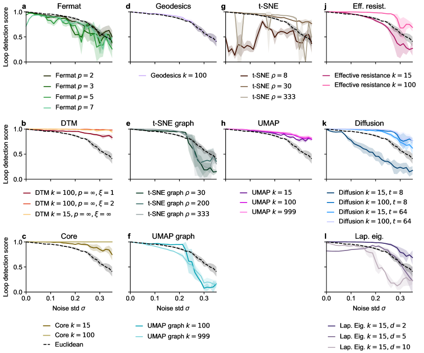
Figure S5: Loop detection score for persistent homology with various distances on a noisy ring in ambient $\mathbb{R}^{2}$. Our code for finding the geodesics for $k=15$ did not terminate.

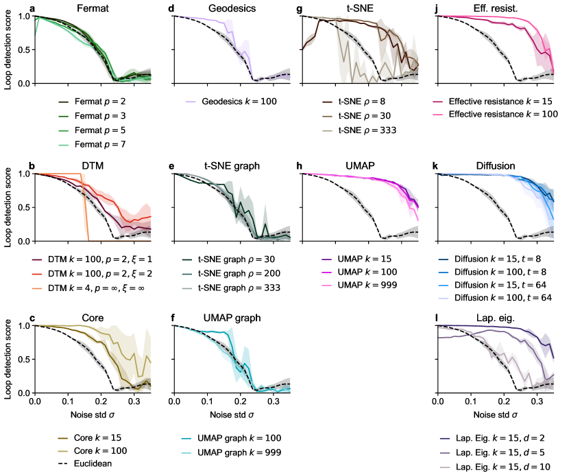
Figure S6: Loop detection score for persistent homology with various distances on a noisy ring in ambient $\mathbb{R}^{50}$. No filtering was used for this figure.

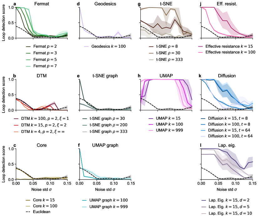
Figure S7: Loop detection score for persistent homology with various distances on the noisy eyeglasses dataset in ambient $\mathbb{R}^{50}$.

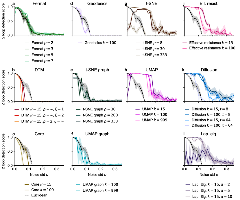
Figure S8: 2 loop detection score for persistent homology with various distances on two interlinked rings in ambient $\mathbb{R}^{50}$.

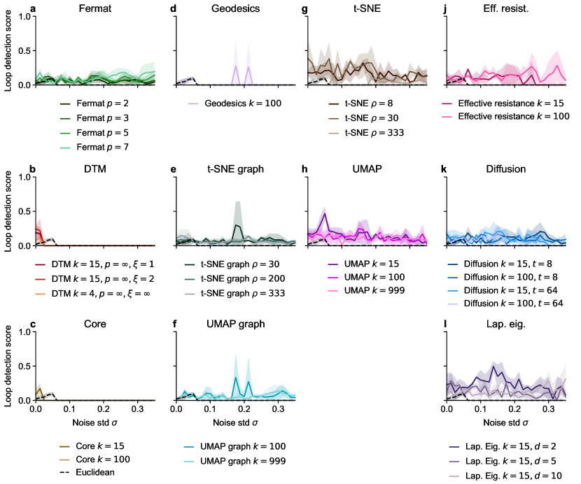
Figure S9: Loop detection score for persistent homology with various distances on a noisy sphere in ambient $\mathbb{R}^{50}$. Most methods pass this negative control.

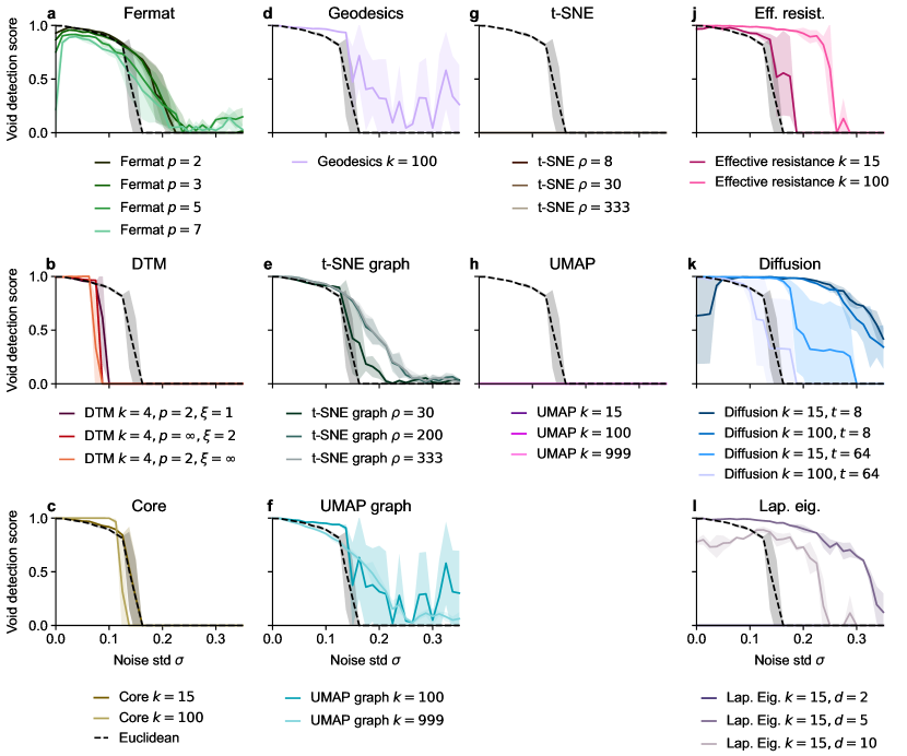
Figure S10: Void detection score for persistent homology with various distances on a noisy sphere in ambient $\mathbb{R}^{50}$. Methods relying on 2D embeddings do not find the loop for any noise level.

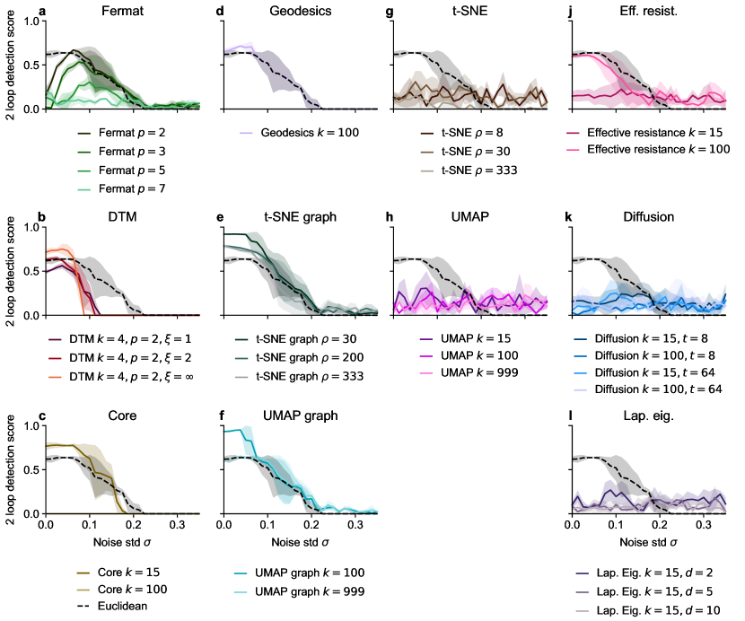
Figure S11: 2 loop detection score for persistent homology with various distances on a noisy torus in ambient $\mathbb{R}^{50}$.

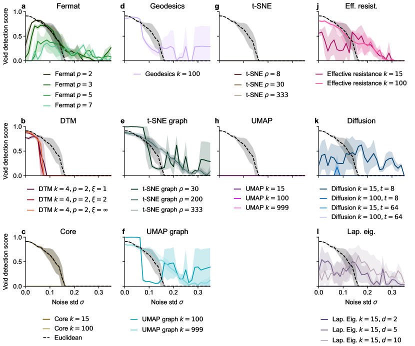
Figure S12: Void detection score for persistent homology with various distances on a noisy torus in ambient $\mathbb{R}^{50}$. Methods relying on 2D embeddings do no find the void for any noise level.

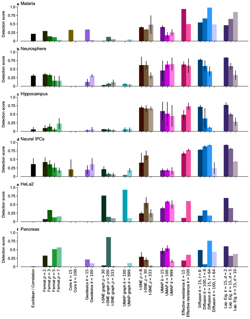
Figure S13: Detection scores for all hyperparameter settings for all six single-cell datasets. We omitted DTM as all settings got filtered on all datasets. The black bar refers to correlation distance on the Malaria dataset and to Euclidean distance on the others. Extension of Figure 9.

References

- Aktas et al. (2019) Mehmet E. Aktas, Esra Akbas, and Ahmed El Fatmaoui. Persistence homology of networks: methods and applications. Applied Network Science, 4(1):1–28, 2019.
- Anai et al. (2020) Hirokazu Anai, Frédéric Chazal, Marc Glisse, Yuichi Ike, Hiroya Inakoshi, Raphaël Tinarrage, and Yuhei Umeda. DTM-based filtrations. In Topological Data Analysis: The Abel Symposium 2018, pp. 33–66. Springer, 2020.
- Bastidas-Ponce et al. (2019) Aimée Bastidas-Ponce, Sophie Tritschler, Leander Dony, Katharina Scheibner, Marta Tarquis-Medina, Ciro Salinno, Silvia Schirge, Ingo Burtscher, Anika Böttcher, Fabian J Theis, et al. Comprehensive single cell mRNA profiling reveals a detailed roadmap for pancreatic endocrinogenesis. Development, 146(12):dev173849, 2019.
- Bauer (2021) Ulrich Bauer. Ripser: efficient computation of Vietoris–Rips persistence barcodes. Journal of Applied and Computational Topology, 5(3), 2021.
- Belkin & Niyogi (2002) Mikhail Belkin and Partha Niyogi. Laplacian Eigenmaps and Spectral Techniques for Embedding and Clustering. In Advances in Neural Information Processing Systems, volume 14, pp. 585–591, 2002.
- Bendich et al. (2011) Paul Bendich, Taras Galkovskyi, and John Harer. Improving homology estimates with random walks. Inverse Problems, 27(12):124002, 2011.
- Böhm et al. (2022) Jan Niklas Böhm, Philipp Berens, and Dmitry Kobak. Attraction-Repulsion Spectrum in Neighbor Embeddings. Journal of Machine Learning Research, 23(95):1–32, 2022.
- Braun et al. (2022) Emelie Braun, Miri Danan-Gotthold, Lars E Borm, Elin Vinsland, Ka Wai Lee, Peter Lönnerberg, Lijuan Hu, Xiaofei Li, Xiaoling He, Žaneta Andrusivová, et al. Comprehensive cell atlas of the first-trimester developing human brain. BioRxiv, pp. 2022–10, 2022.
- Brugnone et al. (2019) Nathan Brugnone, Alex Gonopolskiy, Mark W Moyle, Manik Kuchroo, David van Dijk, Kevin R Moon, Daniel Colon-Ramos, Guy Wolf, Matthew J Hirn, and Smita Krishnaswamy. Coarse Graining of Data via Inhomogeneous Diffusion Condensation. In 2019 IEEE International Conference on Big Data (Big Data), pp. 2624–2633. IEEE, 2019.
- Campello et al. (2015) Ricardo JGB Campello, Davoud Moulavi, Arthur Zimek, and Jörg Sander. Hierarchical Density Estimates for Data Clustering, Visualization, and Outlier Detection. ACM Transactions on Knowledge Discovery from Data (TKDD), 10(1):1–51, 2015.
- Chari & Pachter (2023) Tara Chari and Lior Pachter. The specious art of single-cell genomics. PLOS Computational Biology, 19(8):e1011288, 2023.
- Charlier et al. (2021) Benjamin Charlier, Jean Feydy, Joan Alexis Glaunès, François-David Collin, and Ghislain Durif. Kernel Operations on the GPU, with Autodiff, without Memory Overflows. Journal of Machine Learning Research, 22(74):1–6, 2021. URL http://jmlr.org/papers/v22/20-275.html.
- Chazal et al. (2011) Frédéric Chazal, David Cohen-Steiner, and Quentin Mérigot. Geometric Inference for Measures based on Distance Functions. Foundations of Computational Mathematics, 11(6):733–751, 2011.
- Chazal et al. (2015) Frédéric Chazal, Brittany Fasy, Fabrizio Lecci, Bertrand Michel, Alessandro Rinaldo, and Larry Wasserman. Subsampling Methods for Persistent Homology. In International Conference on Machine Learning, pp. 2143–2151. PMLR, 2015.
- Chew et al. (2022) Joyce Chew, Holly Steach, Siddharth Viswanath, Hau-Tieng Wu, Matthew Hirn, Deanna Needell, Matthew D Vesely, Smita Krishnaswamy, and Michael Perlmutter. The Manifold Scattering Transform for High-Dimensional Point Cloud Data. In Topological, Algebraic and Geometric Learning Workshops 2022, pp. 67–78. PMLR, 2022.
- Cohen-Steiner et al. (2005) David Cohen-Steiner, Herbert Edelsbrunner, and John Harer. Stability of Persistence Diagrams. In Proceedings of the twenty-first annual symposium on Computational geometry, pp. 263–271, 2005.
- Coifman & Lafon (2006) Ronald R Coifman and Stéphane Lafon. Diffusion maps. Applied and Computational Harmonic Analysis, 21(1):5–30, 2006.
- Damm (2022) Daria Damm. Core-Distance-Weighted Persistent Homology and its Behavior on Tree-Shaped Data. Master’s thesis, Heidelberg University, 2022.
- Damrich & Hamprecht (2021) Sebastian Damrich and Fred A Hamprecht. On UMAP’s True Loss Function. In Advances in Neural Information Processing Systems, volume 34, pp. 5798–5809, 2021.
- Doyle & Snell (1984) Peter G Doyle and J Laurie Snell. Random Walks and Electric Networks, volume 22. American Mathematical Soc., 1984.
- Edelsbrunner et al. (2002) Edelsbrunner, Letscher, and Zomorodian. Topological Persistence and Simplification. Discrete & Computational Geometry, 28:511–533, 2002.
- Fernández et al. (2023) Ximena Fernández, Eugenio Borghini, Gabriel Mindlin, and Pablo Groisman. Intrinsic Persistent Homology via Density-based Metric Learning. Journal of Machine Learning Research, 24(75):1–42, 2023.
- Flores-Bautista & Thomson (2023) Emanuel Flores-Bautista and Matt Thomson. Unraveling cell differentiation mechanisms through topological exploration of single-cell developmental trajectories. bioRxiv, pp. 2023–07, 2023.
- Fouss et al. (2007) Francois Fouss, Alain Pirotte, Jean-Michel Renders, and Marco Saerens. Random-walk Computation of Similarities between Nodes of a Graph with Application to Collaborative Recommendation. IEEE Transactions on knowledge and data engineering, 19(3):355–369, 2007.
- Fouss et al. (2016) François Fouss, Marco Saerens, and Masashi Shimbo. Algorithms and Models for Network Data and Link Analysis. Cambridge University Press, 2016.
- Gardner et al. (2022) Richard J Gardner, Erik Hermansen, Marius Pachitariu, Yoram Burak, Nils A Baas, Benjamin A Dunn, May-Britt Moser, and Edvard I Moser. Toroidal topology of population activity in grid cells. Nature, 602(7895):123–128, 2022.
- Gower & Ross (1969) John C Gower and Gavin JS Ross. Minimum Spanning Trees and Single Linkage Cluster Analysis. Journal of the Royal Statistical Society: Series C (Applied Statistics), 18(1):54–64, 1969.
- Groisman et al. (2022) Pablo Groisman, Matthieu Jonckheere, and Facundo Sapienza. Nonhomogeneous Euclidean first-passage percolation and distance learning. Bernoulli, 28(1):255–276, 2022.
- Haghverdi et al. (2015) Laleh Haghverdi, Florian Buettner, and Fabian J Theis. Diffusion maps for high-dimensional single-cell analysis of differentiation data. Bioinformatics, 31(18):2989–2998, 2015.
- Hajij et al. (2018) Mustafa Hajij, Bei Wang, Carlos Scheidegger, and Paul Rosen. Visual Detection of Structural Changes in Time-Varying Graphs using Persistent Homology. In 2018 IEEE Pacific Visualization Symposium (pacificvis), pp. 125–134. IEEE, 2018.
- Hatcher (2002) Allen Hatcher. Algebraic Topology. Cambridge University Press, 2002.
- Hermansen et al. (2022) Erik Hermansen, David Alexander Klindt, and Benjamin Adric Dunn. Uncovering 2-D toroidal representations in grid cell ensemble activity during 1-D behavior. bioRxiv, pp. 2022–11, 2022.
- Hinton & Roweis (2002) Geoffrey E Hinton and Sam Roweis. Stochastic Neighbor Embedding. In Advances in Neural Information Processing Systems, volume 15, pp. 857–864, 2002.
- Howick et al. (2019) Virginia M Howick, Andrew JC Russell, Tallulah Andrews, Haynes Heaton, Adam J Reid, Kedar Natarajan, Hellen Butungi, Tom Metcalf, Lisa H Verzier, Julian C Rayner, et al. The Malaria Cell Atlas: Single parasite transcriptomes across the complete plasmodium life cycle. Science, 365(6455):eaaw2619, 2019.
- Hu et al. (2019) Xiaoling Hu, Fuxin Li, Dimitris Samaras, and Chao Chen. Topology-Preserving Deep Image Segmentation. Advances in Neural Information Processing Systems, 32, 2019.
- Jia & Chen (2022) Junbo Jia and Luonan Chen. Single-cell RNA sequencing data analysis based on non-uniform - neighborhood network. Bioinformatics, 38(9):2459–2465, 2022.
- Kuchroo et al. (2023) Manik Kuchroo, Marcello DiStasio, Eric Song, Eda Calapkulu, Le Zhang, Maryam Ige, Amar H Sheth, Abdelilah Majdoubi, Madhvi Menon, Alexander Tong, et al. Single-cell analysis reveals inflammatory interactions driving macular degeneration. Nature Communications, 14(1):2589, 2023.
- Lamar-León et al. (2012) Javier Lamar-León, Edel B Garcia-Reyes, and Rocio Gonzalez-Diaz. Human Gait Identification Using Persistent Homology. In Progress in Pattern Recognition, Image Analysis, Computer Vision, and Applications: 17th Iberoamerican Congress, CIARP 2012, Buenos Aires, Argentina, September 3-6, 2012. Proceedings 17, pp. 244–251. Springer, 2012.
- Lee et al. (2017) Yongjin Lee, Senja D Barthel, Paweł Dłotko, S Mohamad Moosavi, Kathryn Hess, and Berend Smit. Quantifying similarity of pore-geometry in nanoporous materials. Nature Communications, 8(1):15396, 2017.
- Lopez et al. (2018) Romain Lopez, Jeffrey Regier, Michael B Cole, Michael I Jordan, and Nir Yosef. Deep generative modeling for single-cell transcriptomics. Nature Methods, 15(12):1053–1058, 2018.
- Luke (1969) Yudell L Luke. Special Functions and Their Approximations: vol. 2. Academic Press, 1969.
- Masoomy et al. (2021) Hosein Masoomy, Behrouz Askari, Samin Tajik, Abbas K Rizi, and G Reza Jafari. Topological analysis of interaction patterns in cancer-specific gene regulatory network: Persistent homology approach. Scientific Reports, 11(1):16414, 2021.
- McInnes et al. (2018) Leland McInnes, John Healy, and James Melville. UMAP: Uniform Manifold Approximation and Projection for Dimension Reduction. arXiv preprint arXiv:1802.03426, 2018.
- Mémoli et al. (2022) Facundo Mémoli, Zhengchao Wan, and Yusu Wang. Persistent Laplacians: properties, algorithms and implications. SIAM Journal on Mathematics of Data Science, 4(2):858–884, 2022.
- Moon et al. (2019) Kevin R Moon, David van Dijk, Zheng Wang, Scott Gigante, Daniel B Burkhardt, William S Chen, Kristina Yim, Antonia van den Elzen, Matthew J Hirn, Ronald R Coifman, et al. Visualizing structure and transitions in high-dimensional biological data. Nature Biotechnology, 37(12):1482–1492, 2019.
- Moore et al. (2023) Jessica L Moore, Dhananjay Bhaskar, Feng Gao, Catherine Matte-Martone, Shuangshuang Du, Elizabeth Lathrop, Smirthy Ganesan, Lin Shao, Rachael Norris, Nil Campamà Sanz, et al. Cell cycle controls long-range calcium signaling in the regenerating epidermis. Journal of Cell Biology, 222(7):e202302095, 2023.
- Mukherjee et al. (2022) Soham Mukherjee, Darren Wethington, Tamal K Dey, and Jayajit Das. Determining clinically relevant features in cytometry data using persistent homology. PLoS Computational Biology, 18(3):e1009931, 2022.
- Naitzat et al. (2020) Gregory Naitzat, Andrey Zhitnikov, and Lek-Heng Lim. Topology of deep neural networks. Journal of Machine Learning Research, 21(1):7503–7542, 2020.
- Petenkaya et al. (2022) Aydolun Petenkaya, Farid Manuchehrfar, Constantinos Chronis, and Jie Liang. Identifying Transient Cells During Reprogramming via Persistent Homology. In 2022 44th Annual International Conference of the IEEE Engineering in Medicine & Biology Society (EMBC), pp. 2920–2923. IEEE, 2022.
- Petri et al. (2013) Giovanni Petri, Martina Scolamiero, Irene Donato, and Francesco Vaccarino. Networks and Cycles: A Persistent Homology Approach to Complex Networks. In Proceedings of the European Conference on Complex Systems 2012, pp. 93–99. Springer, 2013.
- Poličar et al. (2019) Pavlin G. Poličar, Martin Stražar, and Blaž Zupan. openTSNE: a modular Python library for t-SNE dimensionality reduction and embedding. bioRxiv, 2019.
- Reid et al. (2018) Adam J Reid, Arthur M Talman, Hayley M Bennett, Ana R Gomes, Mandy J Sanders, Christopher JR Illingworth, Oliver Billker, Matthew Berriman, and Mara KN Lawniczak. Single-cell RNA-seq reveals hidden transcriptional variation in malaria parasites. elife, 7:e33105, 2018.
- Rieck et al. (2018) Bastian Rieck, Matteo Togninalli, Christian Bock, Michael Moor, Max Horn, Thomas Gumbsch, and Karsten Borgwardt. Neural persistence: A complexity measure for deep neural networks using algebraic topology. In International Conference on Learning Representations, 2018.
- Rizvi et al. (2017) Abbas H Rizvi, Pablo G Camara, Elena K Kandror, Thomas J Roberts, Ira Schieren, Tom Maniatis, and Raul Rabadan. Single-cell topological RNA-seq analysis reveals insights into cellular differentiation and development. Nature Biotechnology, 35(6):551–560, 2017.
- Robinson & Oshlack (2010) Mark D Robinson and Alicia Oshlack. A scaling normalization method for differential expression analysis of RNA-seq data. Genome Biology, 11(3):1–9, 2010.
- Roweis & Saul (2000) Sam T Roweis and Lawrence K Saul. Nonlinear Dimensionality Reduction by Locally Linear Embedding. Science, 290(5500):2323–2326, 2000.
- Schwabe et al. (2020) Daniel Schwabe, Sara Formichetti, Jan Philipp Junker, Martin Falcke, and Nikolaus Rajewsky. The transcriptome dynamics of single cells during the cell cycle. Molecular Systems Biology, 16(11):e9946, 2020.
- Singh et al. (2007) Gurjeet Singh, Facundo Mémoli, Gunnar E Carlsson, et al. Topological Methods for the Analysis of High Dimensional Data Sets and 3D Object Recognition. PBG@ Eurographics, 2:091–100, 2007.
- Tenenbaum et al. (2000) Joshua B Tenenbaum, Vin De Silva, and John C Langford. A Global Geometric Framework for Nonlinear Dimensionality Reduction. Science, 290(5500):2319–2323, 2000.
- Turkes et al. (2022) Renata Turkes, Guido F Montufar, and Nina Otter. On the Effectiveness of Persistent Homology. Advances in Neural Information Processing Systems, 35:35432–35448, 2022.
- van der Maaten & Hinton (2008) Laurens van der Maaten and Geoffrey Hinton. Visualizing data using t-SNE. Journal of Machine Learning Research, 9(11):2579–2605, 2008.
- Vishwanath et al. (2020) Siddharth Vishwanath, Kenji Fukumizu, Satoshi Kuriki, and Bharath K Sriperumbudur. Robust Persistence Diagrams using Reproducing Kernels. Advances in Neural Information Processing Systems, 33:21900–21911, 2020.
- von Luxburg et al. (2010a) Ulrike von Luxburg, Agnes Radl, and Matthias Hein. Getting lost in space: Large sample analysis of the resistance distance. Advances in Neural Information Processing Systems, 23, 2010a.
- von Luxburg et al. (2010b) Ulrike von Luxburg, Agnes Radl, and Matthias Hein. Hitting and commute times in large graphs are often misleading. arXiv preprint arXiv:1003.1266, 2010b. version 1 from Mar 05.
- von Luxburg et al. (2014) Ulrike von Luxburg, Agnes Radl, and Matthias Hein. Hitting and Commute Times in Large Random Neighborhood Graphs. Journal of Machine Learning Research, 15(1):1751–1798, 2014.
- Wang et al. (2020) Menglun Wang, Zixuan Cang, and Guo-Wei Wei. A topology-based network tree for the prediction of protein–protein binding affinity changes following mutation. Nature Machine Intelligence, 2(2):116–123, 2020.
- Wang et al. (2023) Shu Wang, Eduardo D Sontag, and Douglas A Lauffenburger. What cannot be seen correctly in 2D visualizations of single-cell ‘omics data? Cell Systems, 14(9):723–731, 2023.
- Zheng et al. (2022) Shijie C Zheng, Genevieve Stein-O’Brien, Jonathan J Augustin, Jared Slosberg, Giovanni A Carosso, Briana Winer, Gloria Shin, Hans T Bjornsson, Loyal A Goff, and Kasper D Hansen. Universal prediction of cell-cycle position using transfer learning. Genome Biology, 23(1):1–27, 2022.
- Zomorodian & Carlsson (2004) Afra Zomorodian and Gunnar Carlsson. Computing Persistent Homology. In Proceedings of the twentieth annual symposium on Computational geometry, pp. 347–356, 2004.