Isogeometric collocation for solving the biharmonic equation over planar multi-patch domains
Abstract
We present an isogeometric collocation method for solving the biharmonic equation over planar bilinearly parameterized multi-patch domains. The developed approach is based on the use of the globally -smooth isogeometric spline space [34] to approximate the solution of the considered partial differential equation, and proposes as collocation points two different choices, namely on the one hand the Greville points and on the other hand the so-called superconvergent points. Several examples demonstrate the potential of our collocation method for solving the biharmonic equation over planar multi-patch domains, and numerically study the convergence behavior of the two types of collocation points with respect to the -norm as well as to equivalents of the -seminorms for . In the studied case of spline degree , the numerical results indicate in case of the Greville points a convergence of order independent of the considered (semi)norm, and show in case of the superconvergent points an improved convergence of order for all (semi)norms except for the equivalent of the -seminorm, where the order is anyway optimal.
keywords:
isogeometric analysis; collocation; superconvergent points; fourth order continuity; multi-patch domain; biharmonic equationMSC:
[2010] 65N35 , 65D17 , 68U071 Introduction
Isogeometric Analysis (IgA) is a numerical framework for solving a partial differential equation (PDE) by employing the same spline or NURBS functions to represent the geometry of the computational domain as well as the numerical solution of the considered PDE [12, 21]. The most common technique in IgA is to transform the original problem (also called strong form of the PDE) into its weak form and to solve the weak form by means of the Galerkin method. The benefit of this approach is that the numerical solution of the weak form can be of (much) lower regularity than the solution of the given strong form. However, the method is based on the evaluation of integrals of (rational) functions of high degree, which requires high computational costs of the matrix assembly routines. Furthermore, consistency, robustness and order of convergence are important issues that have to be considered carefully for each numerical integration technique. An important progress has been achieved in the last years (e.g. [9, 16, 23, 25, 38, 43]), but numerical integration still remains an issue. Another approach in IgA, which we will follow in this work, is to solve the given strong form of the PDE directly via the collocation method. In this way no integration is needed and matrix assembly is much faster, but the method requires spaces of higher smoothness like and -smooth isogeometric spline functions for second and fourth order PDEs, respectively.
Considering planar multi-patch domains with possible extraordinary vertices like in this paper, globally -smooth () isogeometric spline functions are usually constructed by means of the concept of geometric continuity of multi-patch surfaces [44] using the fact that an isogeometric function is -smooth if and only if the associated multi-patch graph surface is -smooth [19, 35]. While for several techniques exist, see the survey articles [22, 27] for more details, there are just a few methods available for , namely the constructions [30, 29, 31, 32, 50] for and the approach [34] for an arbitrary , which includes the case needed for solving the biharmonic equation in strong form via collocation.
Besides multi-patch quadrangular domains, triangulations can be used to generate -smooth spline spaces over complex domains. The book [37] gives an overview of different techniques to model such smooth spline spaces, and provides a detailed bibliography on this topic. Some recent constructions of -smooth spline spaces on triangulations using polynomial macro-element spaces and Powell-Sabin splits can be find e.g. in [49, 20].
The problem of isogeometric collocation has been firstly explored in [3] for solving second order PDEs on a single patch. Thereby, an important issue in isogeometric collocation is the selection of the collocation points, since it affects the convergence behavior of the numerical solution. E.g. for second order problems in case of odd spline degrees , the application of Greville points (abscissae) leads to a convergence of order with respect to -refinement independent of considering the , or -error [3], but the use of so-called superconvergent (Cauchy Galerkin) points [1, 17, 41] improves this convergence to an order of ( for [17]) and for the and -error, respectively. Also for solving fourth order PDEs, Greville and superconvergent points are mainly used. So far, the numerical comparison of the convergence behavior between the two different types of collocation points have been performed just for the norm [17], where for odd spline degrees the superconvergent points show again a better convergence behavior, namely a convergence of order compared to for the Greville points.
While in case of one-patch domains, isogeometric collocation has been already extensively used for solving second and fourth order problems such as the Poisson’s equation, e.g. [1, 3, 14, 17, 41, 48], problems of linear and nonlinear elasticity, elastostatistics and elastodynamics, e.g. [1, 4, 13, 14, 17, 15, 24, 46, 42, 48], acoustics problems, e.g. [5, 2, 51], the Reissner-Mindlin shell problem, e.g. [36], beam problems, e.g. [45, 7, 39], the biharmonic equation/Kirchhoff plate problem, e.g. [10, 45, 17, 40], the Kirchhoff-Love shell problem, e.g. [40] and phase-field models, e.g. [18, 47], in case of multi-patch domains, the number of existing work is small, and is further limited to the solving of second order problems, namely to the Poisson’s equation [33] as well as to elasticity problems [4, 24]. In the case of multi-patch domains, two different strategies have been used for solving the considered second order PDEs. The technique [33] employs the globally -smooth isogeometric spline space [32] as discretization space for the Poisson’s equation, which allows the direct solving of the strong form of the second order PDE. In contrast, the methods [4, 24] employ spline spaces, which are not globally -smooth having a lower regularity at the patch interfaces, and require therefore a special treatment at the patch interface in the collocation procedure.
This paper extends the multi-patch isogeometric collocation method [33] for second order problems to the solving of fourth order PDEs demonstrated on the basis of the biharmonic equation. The presented approach uses the globally -smooth isogeometric spline space [34] to solve the biharmonic equation over bilinearly parameterized multi-patch domains in a strong form, i.e. to compute a -smooth numerical solution of the PDE. Two different choices of collocation points, given by the Greville points as well as by a particular family of superconvergent points, are numerically studied for the case of the odd spline degree and inner patch regularity , which is the configuration with the lowest possible degree for the -smooth spline space [34]. The convergence behavior with respect to -refinement is not only investigated for the -norm as in [17, 40], but also for (equivalents to) the -seminorms for . The numerical results indicate in case of the Greville points a convergence of order independent of the considered norm, and show in case of the superconvergent points an improved convergence of order for all (semi)norms except for the equivalent of the -seminorm, where the order is anyway optimal. Furthermore, it is demonstrated that the rates of convergence for a multi-patch domain coincide with the ones for a one-patch domain.
The remainder of the paper is organized as follows. Section 2 introduces the general framework for solving the biharmonic equation over planar bilinear multi-patch domains via isogeometric collocation. For this purpose, we describe the used multi-patch structure of the domain, explain the general concept of -smooth isogeometric spline functions over planar bilinear multi-patch domains, and present the multi-patch isogeometric collocation approach for solving the biharmonic equation. In Section 3, we determine the final collocation method by specifying on the one hand the used -smooth isogeometric discretization space, namely the -smooth spline space [34], to represent the -smooth approximation of the solution of the biharmonic equation, and by introducing on the other hand two possible choices of collocation points. Section 4 presents several numerical examples, which study the convergence behavior under -refinement with respect to the -norm as well as to (equivalents of) the -seminorms for , and which demonstrate the power of our collocation method to solve the biharmonic equation over bilinearly parameterized multi-patch domains. Finally, we conclude the paper in Section 5.
2 Multi-patch isogeometric collocation for the biharmonic equation
We will describe the general framework for performing isogeometric collocation for solving the biharmonic equation over planar bilinearly parameterized multi-patch domains. This includes the presentation of the considered multi-patch configuration of the domain, the introduction of the concept of -smooth isogeometric spline functions over these multi-patch domains as well as the development of the multi-patch isogeometric collocation technique for solving the biharmonic equation.
2.1 The multi-patch configuration of the domain
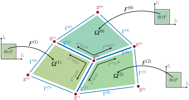
Let be an open and connected planar domain, whose closure is the multi-patch domain with open quadrilateral patches , , which can be further represented as the disjoint union of the open patches , , of open edges , , and of vertices , , i.e.
where denotes the disjoint union of sets, and where , and are the index sets of the indices of the patches , edges and vertices , respectively. The index sets and are further divided into and , where and collect the indices of the inner and boundary edges , respectively, and where and contain the indices of the inner and boundary vertices , respectively. We will assume that the closures of any two patches and , , have either an empty intersection, i.e. , possess exactly one common vertex, i.e. for an , or share the closure of a common inner edge, i.e. for an . Furthermore, we will assume that each patch is parameterized by a bilinear, bijective and regular geometry mapping ,
such that , cf. Fig. 1.
2.2 The concept of -smooth isogeometric functions over bilinear multi-patch domains
Let be the univariate spline space of degree , regularity and mesh size defined on the unit interval and constructed from the uniform open knot vector
where is the number of different inner knots. Furthermore, let be the tensor-product spline space on the unit-square , and let and with , and , the B-splines of the spline spaces and , respectively. Since the geometry mappings , , are bilinearly parameterized, we trivially have that
The space of -smooth isogeometric spline functions over the multi-patch domain is given as
where
is the space of isogeometric spline functions over the multi-patch domain . An isogeometric spline function belongs to the space if and only if for any two neighboring patches and , , with the common inner edge , , the associated graph surface patches and , with the spline functions , , are -smooth across their common interface, cf. [19, 35]. An equivalent condition to the -smoothness of the two neighboring graph surface patches is that the two associated spline functions and satisfy for all
| (1) |
with
where the functions , are called gluing functions, and are linear polynomials defined as
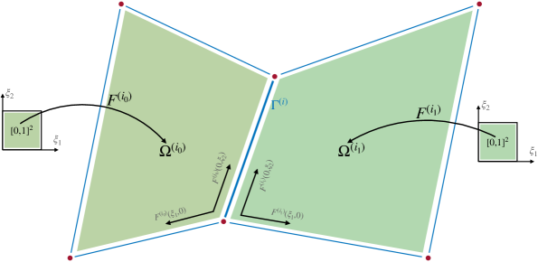
and , , are the Jacobians of , assuming without loss of generality that the two corresponding geometry mappings and are parameterized as shown in Fig. 2, cf. [34, Theorem 2]. Moreover, we have and due to the regularity of the geometry mappings and , and can select e.g. by minimizing cf. [32]. Using the -smoothness conditions (1), the space can be now described as
2.3 Isogeometric collocation for the biharmonic equation
The goal is to find , , which solves the biharmonic equation
| (2) | ||||
where and are sufficiently smooth functions. We will use the concept of isogeometric collocation to compute a -smooth approximation of the solution , where is a suitable discretization space. For this we need a set of global collocation points , , which are further separated into inner collocation points , , and boundary collocation points , . Inserting these points into (2.3), we obtain
| (3) | ||||
To use the isogeometric approach for solving problem , we have first to express each global collocation point with respect to local coordinates via
where
| (4) |
Once we have the local collocation points and , equations (2.3) can be transformed ([6]) to
where
This leads to a linear system for the unknown coefficients of the approximation , where , and is the basis of . In the following section, we will finally determine our isogeometric multi-patch collocation method for solving the biharmonic equation by specifying the used -smooth isogeometric discretization space and by presenting two possible sets of collocation points.
3 The specific setting in the isogeometric collocation
We will present the specific setting for the -smooth isogeometric discretization space and for the set of collocation points in the isogeometric multi-patch collocation approach introduced in the previous section.
3.1 The -smooth isogeometric discretization space
Instead of the entire -smooth isogeometric spline space , which is difficult to construct, we will use as discretization space in the isogeometric collocation method the simpler -smooth subspace
which has been introduced in [34] for an arbitrary smoothness . The construction of the space , which will be summarized111For full details of the construction of the -smooth spline space , we refer to [34]. below, will require a spline degree , an inner patch regularity with as well as a mesh size . In this paper, we will restrict ourselves to the case of the lowest possible spline degree and regularity , namely to and , which further implies .
The -smooth isogeometric spline space is generated as the direct sum of smaller subspaces corresponding to the single patches , , edges , , and vertices , , i.e.,
The single subspaces , and are constructed as the span of corresponding basis functions as demonstrated in the following paragraphs.
The patch subspace
For each patch , , the patch subspace is defined as
with the isogeometric functions
| (6) |
The edge subspace
It has to be distinguished between the case of a boundary and of an inner edge . In case of a boundary edge , , with , , assuming without loss of generality that the boundary edge is given by , the edge subspace is defined as
where the isogeometric functions are given as in (6).
In case of an inner edge , with , , assuming without loss of generality that the two associated geometry mappings and are parameterized as shown in Fig. 2, the edge subspace is given as
where the isogeometric functions have the form
| (7) |
with
| (8) | ||||
and
The vertex subspace
The construction of the vertex subspace differs whether we have an inner or a boundary vertex . Let us first consider the case of an inner vertex , , with patch valency . We assume without loss of generality that all patches , , around the vertex , i.e. , are parameterized as shown in Fig. 1, and relabel the common edges , , by , where is taken modulo . The vertex subspace is now defined as
where the -smooth isogeometric functions in the vicinity of the vertex are given as a linear combination of functions , , , coinciding at their common supports in the vicinity of the vertex , and by subtracting functions , , , which have been added twice. To describe the construction of these functions in more detail, we first consider the isogeometric function of the form
where the functions are given as
with the functions
and with the functions , given in (8). The isogeometric function is -smooth on if the coefficients , satisfy the equations
| (10) |
for and . The equations (10) form a homogeneous system of linear equations, and a basis of the kernel of this system defines now via the corresponding coefficients , the isogeometric functions , , where is the dimension of the kernel of the homogeneous linear system. In our examples in Section 4, we will use the concept of minimal determining sets (cf. [30, 37]) to determine the basis of the kernel.
Let now , , be a boundary vertex with patch valency , and let the two boundary edges be labeled as and . In case of , the construction of the space works analogously as for an inner vertex, except that for the patches and the functions and in (3.1) are the standard B-splines. In case of , the vertex subspace is directly constructed without solving a homogeneous linear system (10). For a patch valency , we assume without loss of generality that the two neighboring patches and , , which contain the vertex and possess the common edge , are parameterized as shown in Fig. 2 and that the vertex is further given as . The vertex subspace is then constructed as
with
where the functions , , and are defined as in (6) and (7), respectively. For a patch valency , we assume without loss of generality that , . Then, the vertex subspace is constructed as
with functions given as in (6).
Remark about the condition for the mesh size
The condition , i.e. for our case and , for the mesh size , ensures the uniform construction of the -smooth spline space for an arbitrary given planar bilinearly parameterized multi-patch domain . Thereby, the required mesh size guarantees that the intersection of two vertex subspaces , , only contains the zero function. However, this condition for the mesh size can be often relaxed. E.g., if the multi-patch domain possesses no inner vertices and no boundary vertices with a patch valency greater than two, cf. Examples 1 and 3, then the -smooth space technically consists just of patch functions and edge functions . Ensuring that each patch or edge function will be only taken once in case it would belong to more than one subspace, the construction of the -smooth space will then work for any mesh size . We can proceed similarly if the multi-patch domain possesses exactly one vertex , , with a patch valency , cf. Example 2. Then we just have additionally to ensure that the patch and edge functions which are involved in the construction of the vertex subspace of the corresponding vertex will not be also taken in another subspace.
3.2 Selection of collocation points
We will select the global collocation points directly via local collocation points for each patch , , as , where are univariate collocation points. For the sake of simplicity, we will use for each patch , , just the same local collocation points with the univariate collocation points . If two or more local collocation points from different patches define the same global collocation point, then we keep just one of these local collocation points, namely the one for the patch with the lowest patch index , cf. (4), to prevent the possible repetition of global collocation points.
In the numerical examples in Section 4, we will study two different choices of univariate collocation points , which will then define the local collocation points for the single patches, and will further determine the global collocation points in the multi-patch isogeometric collocation technique in Section 2.3.
The Greville points
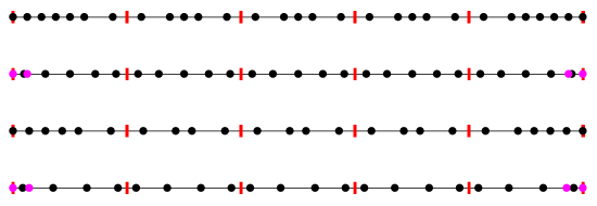
The first choice of points are the Greville points which are defined for an arbitrary and as
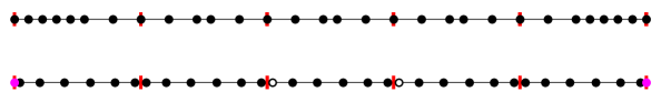
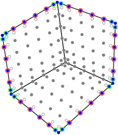
and which are shown for the case , and in Fig. 3 (top row).
The superconvergent points
The second choice of points are the so-called superconvergent points which are defined in our case of the biharmonic equation as the roots of its Galerkin residual . Estimates of these points can be computed by solving the simple biharmonic equation
| (11) |
with some particular function as demonstrated in [17]. Superconvergent points for fourth order problems have been studied so far just for the one-patch case [17, 45, 40], and there only for splines with maximal regularity, i.e. . However, in the multi-patch case the use of splines with maximal regularity is not possible, and splines with a regularity have to be employed instead. Superconvergent points for splines with a lower regularity than have been investigated so far only for the case of second order problems [33], and will be extended below to fourth order problems for the case of the underlying spline space .
Following the approach [17] of studying the Galerkin residual of a particular biharmonic problem (11), we get for the spline space the superconvergent points on each knot span with respect to the reference interval as the roots of the sextic polynomial
Numerical approximations of the six roots are given in Tab. 1 (first row). All univariate superconvergent points are presented in Fig. 3 (bottom row). Since the boundary points of the domain interval are not contained in the set of superconvergent points, they have to be added to the set to be able to impose the required boundary conditions.
To get the same number of collocation points as the dimension of the spline space, it can be necessary to select a proper subset of superconvergent points, or conversely, to add some points to the set of superconvergent points, cf. [41, 33]. In our case the difference between the number of all superconvergent points and the dimension of the underlying spline space is
so we have to omit points. For this purpose, we skip for all most inner knots (at least two away from the boundary) the closest collocation point to the right of the knot, compare Fig. 3 (white points). For special cases , we either add the inner knot (case ) or we add the second and the second last Greville point (case ).
Separation of collocation points
Above, we have explained for the spline space two possible choices of univariate local collocation points , namely the Greville and superconvergent points, where in both cases the number of points coincides with the dimension of the spline space. Recall that the univariate local collocation points define via the local collocation points . Then, each local collocation point for a patch defines via the global collocation point , , taking under consideration, that if the global collocation point would lie on more than one patch, the global collocation point is just selected once, namely for the patch with the lowest patch index , cf. (4).
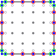
The usage of the multi-patch isogeometric collocation approach presented in Section 2.3 still requires the separation of the set of global collocation points , , into inner collocation points , , and boundary collocation points , . The straightforward separation would be to take all global collocation points which lie on the boundary of the domain as boundary collocation points, and to take the remaining points as inner collocation points. However, this separation would lead even in the one-patch case to an overdetermined linear system, since we would have too many collocation points in total. Therefore, we will follow the separation technique used in [45, 18] for the one-patch case, which will lead in this case to a square linear system, and will extend it to the multi-patch case, where we will obtain just a slightly overdetermined linear system, which will then be solved by means of the least-squares approach in the numerical examples in Section 4. The separation of the collocation points will work as follows. We will omit some of the inner collocation points where the biharmonic equation is imposed, and will choose the boundary collocation points for interpolation of the normal derivatives in a proper way. In the one-patch case, cf. Fig. 4 (left), we will omit the last outer ring of inner collocation points, see Fig. 4 (white points), and we will further omit eight interpolation conditions at the boundary. For the later purpose, we will not interpolate the normal derivatives at the four corner points, and will additionally average the normal derivative equations corresponding to the two boundary points closest to the corner points, see Fig. 4 (green circles). This strategy will be generalized in a straightforward way to the multi-patch case as demonstrated in Fig. 4 (right).
The convergence behavior of the collocation points
For fourth order problems, the convergence behavior of both types of collocation points has been studied so far only with respect to the -norm for the one-patch case and there just using splines with maximal regularity, where for odd spline degrees a convergence of order and for the Greville and superconvergent points, respectively, have been reported, cf. [17, 46]. In the following section, we will first numerically demonstrate for the one-patch case that the convergence behavior of both types of collocation points will be unchanged by employing the spline space with and . Moreover, we will study for this spline space the convergence behavior with respect to (equivalents of) the -seminorms for , where in case of the Greville points a convergence of order for all seminorms will be observed, and where in case of the superconvergent points the convergence will be of order except for the equivalent of the -seminorm with a convergence order . In the multi-patch case, we will present several examples which will indicate for both considered types of collocation points, i.e. the Greville and superconvergent points, that the convergence rates for all (semi)norms will be the same as in the one-patch case.
4 Numerical examples
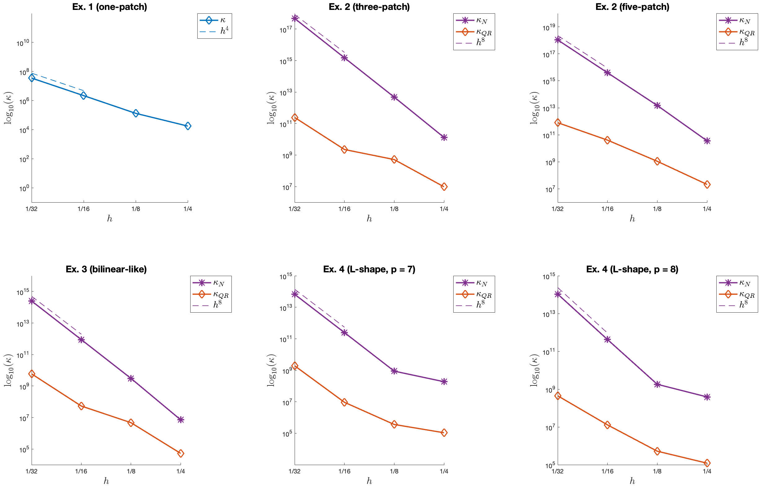
We will demonstrate on the basis of several examples the potential of our isogeometric collocation method for solving the biharmonic equation over planar multi-patch domains, and will study the convergence behavior under -refinement for both types of considered collocation points, namely for the Greville and superconvergent points. While the first example (Example 1) will deal with the one-patch case, the remaining examples (Examples 2–4) will study different instances of multi-patch domains. As already mentioned in the previous section, the use of both sets of collocation points will lead in case of a multi-patch domain (Examples 2–4) to a slightly overdetermined system of linear equations, see Tab. 2 for the dimensions of these resulting collocation matrices. This overdetermined linear system could be solved e.g. by using diagonal scaling ([8]) on a symmetric positive definite matrix obtained by employing the normal system approach or by using QR-decomposition. Condition numbers with estimated growth rates for both approaches and for all considered examples are presented in Fig. 11. Since the QR decomposition approach gives lower condition numbers, we will use this method to construct all multi-patch examples below.
In all examples (Examples 1–4), we will solve the biharmonic equation (2.3), where the right side functions and are obtained from the exact solution
| (12) |
In the first three examples (Examples 1–3), we will employ the -smooth isogeometric spline spaces with a spline degree , with an inner patch regularity and with mesh sizes , , as discretization spaces to compute a -smooth approximation of the solution of the biharmonic equation (2.3), and will denote the resulting space for a specific mesh size by . We will investigate the quality of the obtained approximant with respect to the exact solution (12) by considering the relative errors with respect to the -norm and -seminorm as well as with respect to equivalents (cf. [6]) of the -seminorms, , i.e.
| (13) |
For the sake of brevity, we will refer in this section to the relative errors with respect to the equivalents of the -seminorms, , just as relative errors with respect to the corresponding -seminorms.
Example 1.
We consider the bilinear one-patch domain shown in Fig. 5 (top left). In this case, the -smooth discretization spaces , , , technically consist of only patch functions (cf. last paragraph in Section 3.1), and the resulting linear system (2.3) is a square system. The resulting relative errors (13) by using the Greville and superconvergent points are shown in Fig. 5.
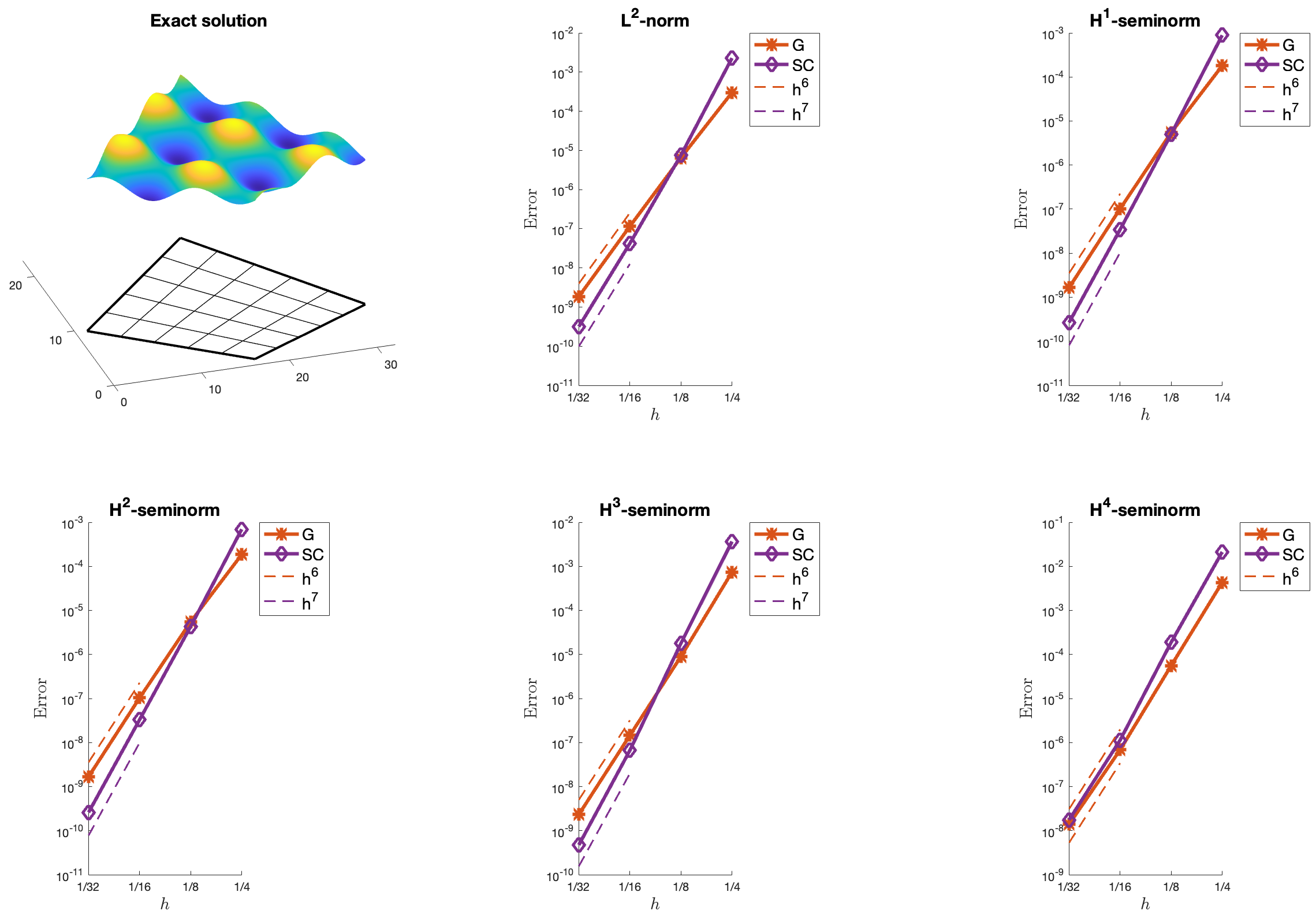
The convergence rate for the relative -error coincides with the known results for splines with maximal regularity, i.e. , for the one-patch case [17, 46], and is in case of odd spline degree of order for the Greville points and of order for the superconvergent points. Furthermore, the error plots indicate the convergence orders with respect to the -seminorms, , where for the Greville points the order remains for all seminorms, while in the case of the superconvergent points the orders are for all the seminorms except for the -seminorm, where is already the best possible one, which would be also obtained in case of the Galerkin approach.
Example 2.
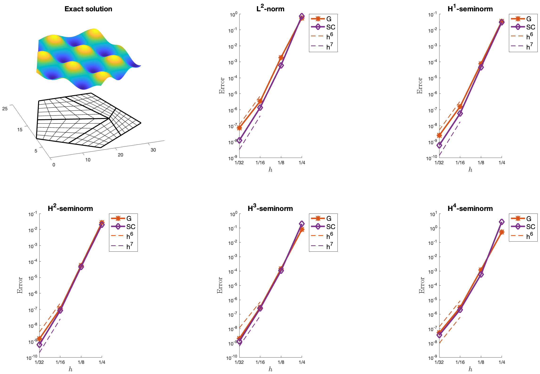
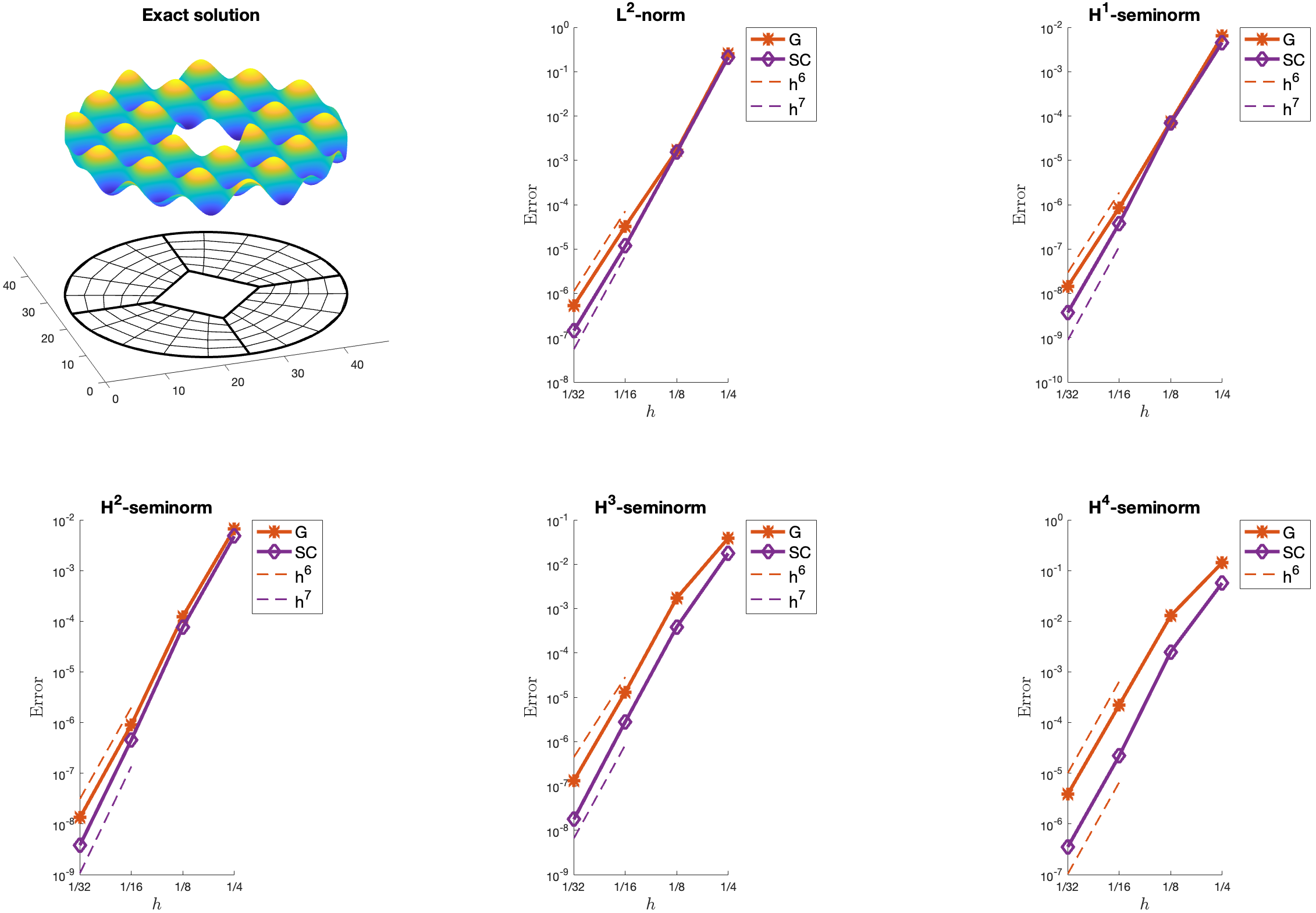
In this example we consider the bilinear three-patch and five patch domains visualized in Fig. 6 (top left) and Fig. 7 (top left), respectively.
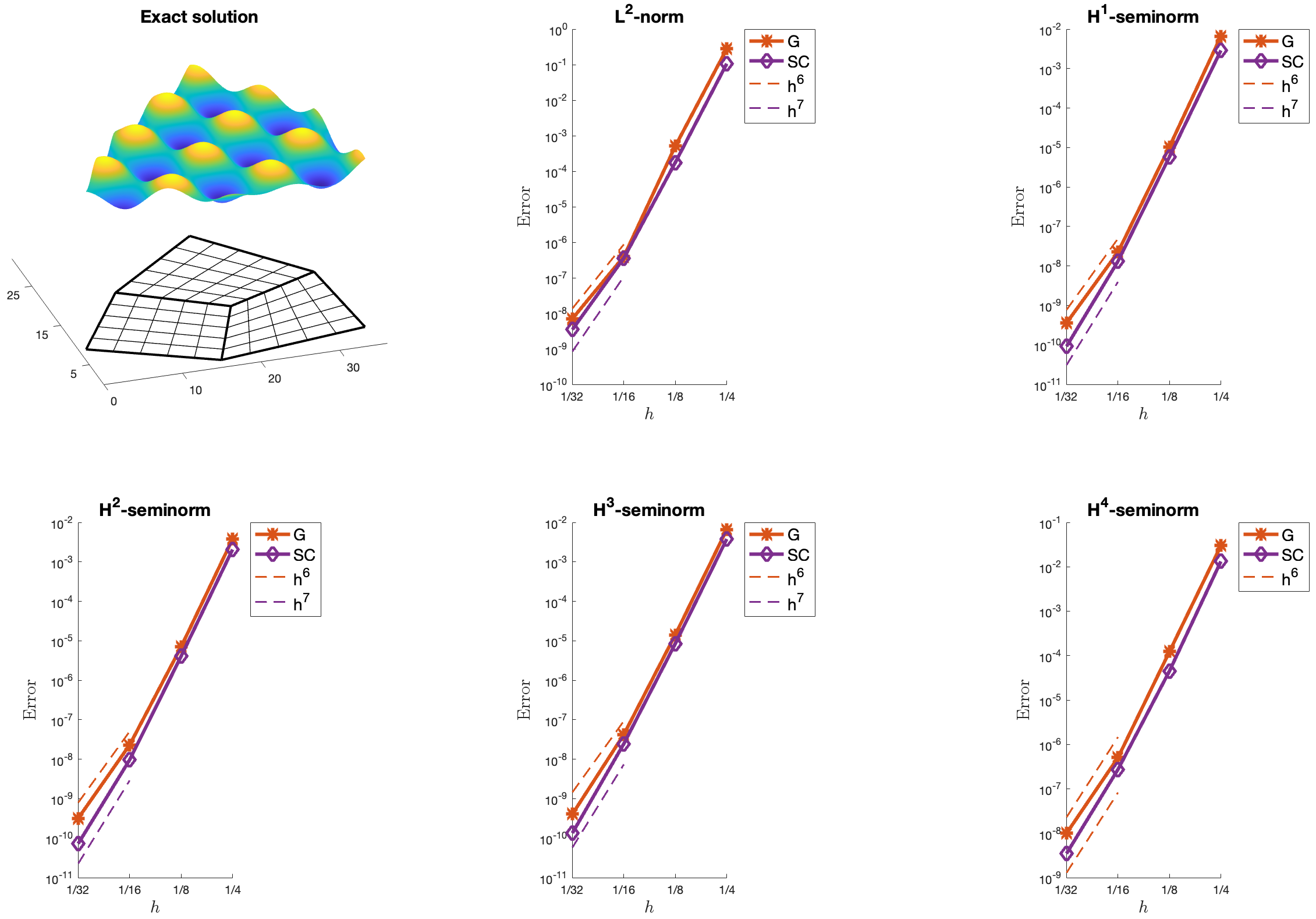
The -smooth discretization spaces , , , are constructed as presented in Section 3.1 following the mentioned adaptation from the last paragraph for the mesh sizes and . Again, we compare the resulting relative errors (13) with respect to the -norm and to -seminorms, , by using the Greville and superconvergent points, see Fig. 6 for the three-patch domain and Fig. 7 for the five-patch domain. The numerical results indicate in case of the Greville points a convergence of order independent of the considered (semi)norm, and show in case of the superconvergent points an improved convergence of order for all (semi)norms except for the -seminorm, where the order is already optimal, which is for all (semi)norms the same convergence behavior as in the one-patch case in Example 1.
Example 3.
We consider now a generalization of bilinear multi-patch domains to the case of bilinear-like multi-patch geometries, see e.g. [11, 31, 34]. These multi-patch parameterizations possess as in the bilinear case linear gluing functions and also allow the construction of globally -smooth isogeometric spline spaces with optimal approximation properties. More precisely, a multi-patch parameterization is called bilinear-like if for any two neighboring patches and , , with , , and corresponding geometry mappings and , , parameterized as in Fig. 2, there exist linear functions , such that
with
The advantage of using bilinear-like multi-patch parameterizations instead of just bilinear multi-patch parameterizations is the possibility to deal with multi-patch domains having curved interfaces and boundaries, see e.g. [26, 27, 28, 34].
We study more precisely the bilinear-like four-patch domain shown in Fig. 8 (top left), that consists of polynomial patches of bi-degree , and possesses a -smooth outer boundary and an inner boundary with sharp corners. The domain can represent a real engineering domain, namely a washer with a square hole. Compared to round washers, square washers have a higher surface area, which improves torque distribution. They help in corrosion resistance and rotation prevention. The -smooth discretization spaces , , technically consist now of only patch and edge functions (cf. last paragraph in Section 3.1). We compare the resulting relative errors (13) with respect to the -norm and with respect to the -seminorms, , by using the Greville and superconvergent points as collocation points, see Fig. 8. Again, the numerical results indicate the same convergence behavior as in the previous examples.
In the last example, we will present a first possible way to slightly reduce the required spline degree of the used discretization space by reducing the regularity of the numerical solution as well, cf. [1]. For this purpose, we will relax the condition of computing a -smooth approximation of the solution of the biharmonic equation by constructing instead just a -smooth approximation. Since the obtained approximant will now be globally only -smooth, we will have to choose the collocation points carefully in order to avoid collocating at the knots and common edges , , where the fourth derivative of the approximant may be discontinuous. Again, we will study the convergence rates of the relative errors (13).
Example 4.
Let be the bilinear two-patch L-shape domain given in Fig. 10 (top left). The goal is to compute via our collocation approach a -smooth approximant of the solution of the biharmonic equation, where is the -smooth isogeometric discretization space [34] for a specific mesh size , , whose construction is similar to the one for the -smooth spline space described in Section 3.1. The -smooth spline space allows the use of underlying spaces with . In this example, we will consider underlying spline spaces with and for both sets of collocation points, namely for the Greville and superconvergent points. Since the regularity is odd and less than , it is easy to see that the Greville points for the two spline spaces and never coincide with inner knots, cf. Fig. 9.
Therefore, we only have to avoid collocating at the common edge of the two-patch domain, where the solution is not -smooth. Similarly as for the case in Section 3.2, we can construct the superconvergent points for the cases and . In the first case, i.e. for the spline space , the superconvergent points on each knot segment (with respect to the reference interval ) are the roots of the quintic polynomial
while in the second case, i.e. for the spline space , we have to take the roots of the quartic polynomial
cf. Tab. 1.
| , | |
|---|---|
| , | |
| , |
Again, we have to find a proper set of superconvergent points whose cardinality coincides with the dimension of the underlying spline space or . In this example, we have to add (in both cases) the first two Greville points at both ends of the domain interval, see Fig. 9. The same strategy has been already used for selecting additional points close to the boundary in [17, 33, 41]. When considering our two-patch domain (Fig. 10, top left), we only have, as for the Greville collocation points, to avoid collocating at the common edge, where the numerical solution is not -smooth.
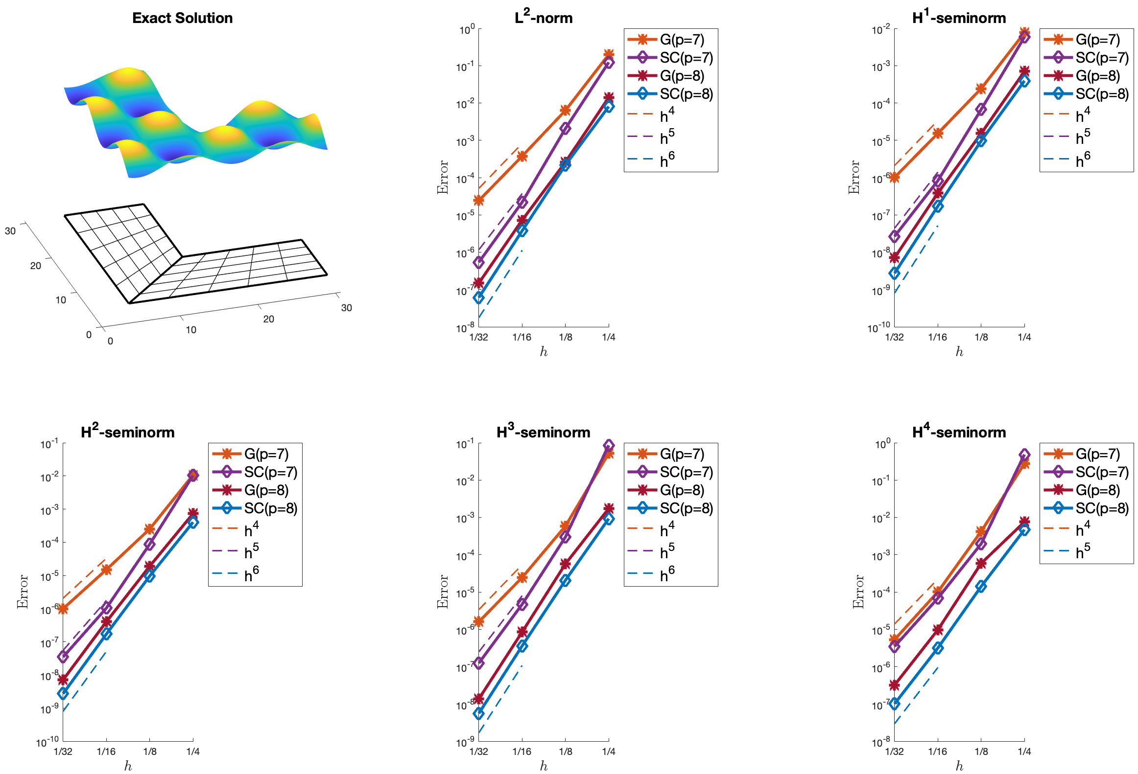
The convergence rates for the relative errors (13) with respect to the -norm and with respect to the -seminorms, , are presented in Fig. 10. For odd spline degree , the orders of convergence coincide with the ones in the previous examples, i.e. they are of order in the case of Greville points, and they are of order for all (semi)norms except for the -seminorm, where the order is , in the case of superconvergent points. For even spline degree , the orders of convergence are the same for the Greville and superconvergent points, namely for the -norm and for the -seminorms, for , and for the -seminorm. Note that the observed convergence behavior with respect to the -norm is for even spline degree again in agreement with the known one-patch result for splines with maximal regularity, cf. [17, 46].
| Case \ | ||||
|---|---|---|---|---|
| Ex. 1 (one-patch) | ||||
| Ex. 2 (three-patch) | ||||
| Ex. 2 (five-patch) | ||||
| Ex. 3 (bilinear-like) | ||||
| Ex. 4 (L-shape, ) | ||||
| Ex. 4 (L-shape, ) |
5 Conclusion
We presented a novel method for solving the biharmonic equation over planar bilinearly parameterized multi-patch domains in strong form, and extended the presented technique on the basis of an example also to the case of bilinear-like multi-patch geometries, which allow the modeling of curved interfaces and boundaries. Our developed isogeometric collocation approach is based on the use of the globally -smooth isogeometric spline space [34] with spline degree to represent the -smooth numerical solution of the biharmonic equation. For the choice of the collocation points, two different sets of points have been proposed, namely the Greville points, and a new family of superconvergent points. We tested both choices on a one-patch domain as well as on several instances of multi-patch domains. For both sets of collocation points, we numerically studied the convergence behavior with respect to the -norm and with respect to (equivalents of) the -seminorms, . For the considered odd spline degree , we observed in case of the Greville points a convergence of order for all (semi)norms, and in case of the superconvergent points an improved convergence of order for all (semi)norms except for the -seminorm, where the order is optimal.
We also studied on the basis of an example a first possibility to slightly reduce the required spline degree of the isogeometric multi-patch discretization space by reducing the regularity of the numerical solution as well. Another strategy and a first possible topic for future research could be to employ functions of degree just in the vicinity of edges and vertices, and to use functions with spline degree in the interior of patches. A further open issue is the following. Since the number of collocation points in the multi-patch case is slightly larger than the dimension of the discretization space, the finding of a set of collocation points with the same cardinality as the dimension of the space would be of interest, too, in order to avoid the necessity of the least-squares method for solving the resulting linear system. In addition, other applications such as the Kirchhoff plate or Kirchhoff-Love shell problem, and the extension of our approach to multi-patch surfaces or to multi-patch volumes could be worth to study, too.
Acknowledgment
The authors wish to thank the anonymous reviewers for their comments that helped to improve the paper. M. Kapl has been partially supported by the Austrian Science Fund (FWF) through the project P 33023-N. V. Vitrih has been partially supported by the Slovenian Research and Innovation Agency (research program P1-0404 and research projects N1-0296, J1-1715, N1-0210 and J1-4414). A. Kosmač has been partially supported by the Slovenian Research and Innovation Agency (research program P1-0404, research project N1-0296 and Young Researchers Grant). This support is gratefully acknowledged.
References
- [1] C. Anitescu, Y. Jia, Y. J. Zhang, and T. Rabczuk. An isogeometric collocation method using superconvergent points. Comput. Methods Appl. Mech. Engrg., 284:1073–1097, 2015.
- [2] E. Atroshchenko, A. Calderon Hurtado, C. Anitescu, and T. Khajah. Isogeometric collocation for acoustic problems with higher-order boundary conditions. Wave Motion, 110:Paper No. 102861, 24, 2022.
- [3] F. Auricchio, L. Beirão da Veiga, T. J. R. Hughes, A. Reali, and G. Sangalli. Isogeometric collocation methods. Math. Models Methods Appl. Sci., 20(11):2075–2107, 2010.
- [4] F. Auricchio, L. Beirão da Veiga, T.J.R. Hughes, A. Reali, and G. Sangalli. Isogeometric collocation for elastostatics and explicit dynamics. Comput. Methods Appl. Mech. Engrg., 249–252:2–14, 2012.
- [5] T. Ayala, J. Videla, C. Anitescu, and E. Atroshchenko. Enriched isogeometric collocation for two-dimensional time-harmonic acoustics. Comput. Methods Appl. Mech. Engrg., 365:113033, 32, 2020.
- [6] A. Bartezzaghi, L. Dedè, and A. Quarteroni. Isogeometric analysis of high order partial differential equations on surfaces. Comput. Methods Appl. Mech. Engrg., 295:446 – 469, 2015.
- [7] L. Beirão da Veiga, C. Lovadina, and A. Reali. Avoiding shear locking for the Timoshenko beam problem via isogeometric collocation methods. Comput. Methods Appl. Mech. Engrg., 241–244:38–51, 2012.
- [8] A. M. Bruaset. A survey of preconditioned iterative methods, volume 328 of Pitman Research Notes in Mathematics Series. Longman Scientific & Technical, Harlow, 1995.
- [9] F. Calabrò, G. Sangalli, and M. Tani.
- [10] H. Casquero, L. Liu, Y. Zhang, A. Reali, and H. Gomez. Isogeometric collocation using analysis-suitable T-splines of arbitrary degree. Comput. Methods Appl. Mech. Engrg., 301:164–186, 2016.
- [11] A. Collin, G. Sangalli, and T. Takacs. Analysis-suitable G1 multi-patch parametrizations for C1 isogeometric spaces. Comput. Aided Geom. Des., 47:93 – 113, 2016.
- [12] J. A. Cottrell, T. J. R. Hughes, and Y. Bazilevs. Isogeometric Analysis: Toward Integration of CAD and FEA. John Wiley & Sons, Chichester, England, 2009.
- [13] J. A. Evans, R. R. Hiemstra, T. J. R. Hughes, and A. Reali. Explicit higher-order accurate isogeometric collocation methods for structural dynamics. Comput. Methods Appl. Mech. Engrg., 338:208–240, 2018.
- [14] F. Fahrendorf, L. De Lorenzis, and H. Gomez. Reduced integration at superconvergent points in isogeometric analysis. Comput. Methods Appl. Mech. Engrg., 328:390–410, 2018.
- [15] F. Fahrendorf, S. Morganti, A. Reali, T. J. R. Hughes, and L. De Lorenzis. Mixed stress-displacement isogeometric collocation for nearly incompressible elasticity and elastoplasticity. Comput. Methods Appl. Mech. Engrg., 369:113112, 48, 2020.
- [16] A. Giust and B. Jüttler.
- [17] H. Gomez and L. De Lorenzis. The variational collocation method. Comput. Methods Appl. Mech. Engrg., 309:152–181, 2016.
- [18] H. Gomez, A. Reali, and G. Sangalli. Accurate, efficient, and (iso)geometrically flexible collocation methods for phase-field models. J. Comput. Phys., 262:153–171, 2014.
- [19] D. Groisser and J. Peters. Matched Gk-constructions always yield Ck-continuous isogeometric elements. Comput. Aided Geom. Des., 34:67–72, 2015.
- [20] J. Grošelj. A normalized representation of super splines of arbitrary degree on Powell-Sabin triangulations. BIT Numerical Mathematics, 56(4):1257–1280, 2016.
- [21] T. J. R. Hughes, J. A. Cottrell, and Y. Bazilevs. Isogeometric analysis: CAD, finite elements, NURBS, exact geometry and mesh refinement. Comput. Methods Appl. Mech. Engrg., 194(39-41):4135–4195, 2005.
- [22] T. J. R. Hughes, G. Sangalli, T. Takacs, and D. Toshniwal. Chapter 8 - smooth multi-patch discretizations in isogeometric analysis. In Andrea Bonito and Ricardo H. Nochetto, editors, Geometric Partial Differential Equations - Part II, volume 22 of Handbook of Numerical Analysis, pages 467–543. Elsevier, 2021.
- [23] T.J.R. Hughes, A. Reali, and G. Sangalli. Efficient quadrature for NURBS-based isogeometric analysis. Computer Methods in Applied Mechanics and Engineering, 199(5):301–313, 2010. Computational Geometry and Analysis.
- [24] Y. Jia, C. Anitescu, Y. J. Zhang, and T. Rabczuk. An adaptive isogeometric analysis collocation method with a recovery-based error estimator. Comput. Methods Appl. Mech. Engrg., 345:52–74, 2019.
- [25] B. Jüttler, A. Mantzaflaris, R. Perl, and M. Rumpf. On numerical integration in isogeometric subdivision methods for pdes on surfaces. Computer Methods in Applied Mechanics and Engineering, 302:131–146, 2016.
- [26] M. Kapl, G. Sangalli, and T. Takacs. Construction of analysis-suitable G1 planar multi-patch parameterizations. Comput.-Aided Des., 97:41–55, 2018.
- [27] M. Kapl, G. Sangalli, and T. Takacs. Isogeometric analysis with C1 functions on unstructured quadrilateral meshes. The SMAI journal of computational mathematics, 5:67–86, 2019.
- [28] M. Kapl, G. Sangalli, and T. Takacs. An isogeometric C1 subspace on unstructured multi-patch planar domains. Comput. Aided Geom. Des., 69:55–75, 2019.
- [29] M. Kapl and V. Vitrih. Space of C2-smooth geometrically continuous isogeometric functions on planar multi-patch geometries: Dimension and numerical experiments. Comput. Math. Appl., 73(10):2319–2338, 2017.
- [30] M. Kapl and V. Vitrih. Space of C2-smooth geometrically continuous isogeometric functions on two-patch geometries. Comput. Math. Appl., 73(1):37–59, 2017.
- [31] M. Kapl and V. Vitrih. Dimension and basis construction for -smooth isogeometric spline spaces over bilinear-like two-patch parameterizations. J. Comput. Appl. Math., 335:289–311, 2018.
- [32] M. Kapl and V. Vitrih. Solving the triharmonic equation over multi-patch planar domains using isogeometric analysis. J. Comput. Appl. Math., 358:385–404, 2019.
- [33] M. Kapl and V. Vitrih. Isogeometric collocation on planar multi-patch domains. Comput. Methods Appl. Mech. Engrg., 360:112684, 2020.
- [34] M. Kapl and V. Vitrih. -smooth isogeometric spline spaces over planar multi-patch parameterizations. Advances in Computational Mathematics, 47:47, 2021.
- [35] M. Kapl, V. Vitrih, B. Jüttler, and K. Birner. Isogeometric analysis with geometrically continuous functions on two-patch geometries. Comput. Math. Appl., 70(7):1518 – 1538, 2015.
- [36] J. Kiendl, E. Marino, and L. De Lorenzis. Isogeometric collocation for the Reissner-Mindlin shell problem. Comput. Methods Appl. Mech. Engrg., 325:645–665, 2017.
- [37] M.-J. Lai and L. L. Schumaker. Spline functions on triangulations, volume 110 of Encyclopedia of Mathematics and its Applications. Cambridge University Press, Cambridge, 2007.
- [38] A. Mantzaflaris and B. Jüttler. Integration by interpolation and look-up for Galerkin-based isogeometric analysis. Computer Methods in Applied Mechanics and Engineering, 284:373–400, 2015. Isogeometric Analysis Special Issue.
- [39] E. Marino, J. Kiendl, and L. De Lorenzis. Explicit isogeometric collocation for the dynamics of three-dimensional beams undergoing finite motions. Comput. Methods Appl. Mech. Engrg., 343:530–549, 2019.
- [40] F. Maurin, F. Greco, L. Coox, D. Vandepitte, and W. Desmet. Isogeometric collocation for Kirchhoff-Love plates and shells. Comput. Methods Appl. Mech. Engrg., 329:396–420, 2018.
- [41] M. Montardini, G. Sangalli, and L. Tamellini. Optimal-order isogeometric collocation at Galerkin superconvergent points. Comput. Methods Appl. Mech. Engrg., 316:741–757, 2017.
- [42] S. Morganti, F. Fahrendorf, L. De Lorenzis, J. A. Evans, T. J. R. Hughes, and A. Reali. Isogeometric collocation: A mixed displacement-pressure method for nearly incompressible elasticity. Computer Modeling in Engineering Sciences, 129(3):1125–1150, 2021.
- [43] M. Pan, B. Jüttler, and A. Giust. Fast formation of isogeometric galerkin matrices via integration by interpolation and look-up. Computer Methods in Applied Mechanics and Engineering, 366:113005, 2020.
- [44] J. Peters. Geometric continuity. In Handbook of computer aided geometric design, pages 193–227. North-Holland, Amsterdam, 2002.
- [45] A. Reali and H. Gomez. An isogeometric collocation approach for Bernoulli-Euler beams and Kirchhoff plates. Comput. Methods Appl. Mech. Engrg., 284:623–636, 2015.
- [46] A. Reali and T. J. R. Hughes. An introduction to isogeometric collocation methods. In Isogeometric Methods for Numerical Simulation, pages 173–204. Springer, 2015.
- [47] D. Schillinger, M. J. Borden, and H. K. Stolarski. Isogeometric collocation for phase-field fracture models. Comput. Methods Appl. Mech. Engrg., 284:583–610, 2015.
- [48] D. Schillinger, J. A. Evans, A. Reali, M. A. Scott, and T. J.R. Hughes. Isogeometric collocation: Cost comparison with Galerkin methods and extension to adaptive hierarchical NURBS discretizations. Comput. Methods Appl. Mech. Engrg., 267:170 – 232, 2013.
- [49] H. Speleers. Construction of normalized B-splines for a family of smooth spline spaces over Powell-Sabin triangulations. Constr. Approx., 37(1):41–72, 2013.
- [50] D. Toshniwal, H. Speleers, R. Hiemstra, and T. J. R. Hughes. Multi-degree smooth polar splines: A framework for geometric modeling and isogeometric analysis. Comput. Methods Appl. Mech. Engrg., 316:1005–1061, 2017.
- [51] E. Zampieri and L. F. Pavarino. Isogeometric collocation discretizations for acoustic wave problems. Comput. Methods Appl. Mech. Engrg., 385:114047, 2021.