OrthoNets: Orthogonal Channel Attention Networks

Abstract

Designing an effective channel attention mechanism implores one to find a lossy-compression method allowing for optimal feature representation. Despite recent progress in the area, it remains an open problem. FcaNet, the current state-of-the-art channel attention mechanism, attempted to find such an information-rich compression using Discrete Cosine Transforms (DCTs). One drawback of FcaNet is that there is no natural choice of the DCT frequencies. To circumvent this issue, FcaNet experimented on ImageNet to find optimal frequencies. We hypothesize that the choice of frequency plays only a supporting role and the primary driving force for the effectiveness of their attention filters is the orthogonality of the DCT kernels. To test this hypothesis, we construct an attention mechanism using randomly initialized orthogonal filters. Integrating this mechanism into ResNet, we create OrthoNet. We compare OrthoNet to FcaNet (and other attention mechanisms) on Birds, MS-COCO, and Places356 and show superior performance. On the ImageNet dataset, our method competes with or surpasses the current state-of-the-art. Our results imply that an optimal choice of filter is elusive and generalization can be achieved with a sufficiently large number of orthogonal filters. We further investigate other general principles for implementing channel attention, such as its position in the network and channel groupings. Our code is publicly available at (https://github.com/hady1011/OrthoNets)

I Introduction

Deep convolutional neural networks have become the standard tool to accomplish many computer vision tasks such as classification, segmentation, and object detection [24, 8]. Their success is attributed to the ability to extract features related to the underlying task. Higher quality features allow for better outputs in the decision space. Hence, improving the quality of these features has become an area of interest in the machine learning community [41, 39, 31]. In this paper, we investigate channel attention mechanisms.

A channel attention mechanism is a module placed throughout the network. Each module takes as input a feature, which has $C$ channels, and outputs a $C$ dimensional attention vector with components in $(0,1)$. By multiplying these outputs with the input feature vector, the features are adapted towards solving the underlying task.

Figure 1: ImageNet accuracy comparison. Our Method outperforms FcaNet using 34 layers and achieves competitive results with 50 and 101 layers while using 10% less parameters and reducing computational cost.

The first channel attention mechanism, introduced by SENet [11], uses Global Average Pooling (GAP) to compress the spatial dimension of each feature channel into a single scalar. To compute the attention vector, the compressed representation is sent through a Multi-Layer Perceptron (MLP) and then through a sigmoid function. The compression stage is referred to as the squeeze. As pointed out in [23], a major weakness of SENet is using a single method (i.e. GAP) to compress each channel. This weakness was removed by FcaNet [23]. They argue that GAP is discarding essential low-frequency information and that generalizing channel attention in the frequency domain by using DCTs, yields more information. Doing so improves channel attention significantly. Based on imperial results, FcaNet chose which Discrete Cosine Transforms (DCTs) to use, thus becoming the state-of-the-art (SOTA) channel attention mechanism.

We hypothesize that the success of FcaNet has less to do with the low-frequency spectral information and is, in fact, due to the orthogonal nature of the DCT compression mappings. To test this hypothesis, we construct a channel attention mechanism using random orthonormal filters to compress the spatial information of each feature. Using our attention mechanisms, we produce networks that outperform FcaNet in object detection and image segmentation tasks. Compared to SOTA, our method achieves competitive or superior results on the ImageNet dataset and achieves top performance for attention mechanisms on Birds and Places365 datasets. We further investigate other general principles for implementing channel attention. The main contributions of this work are summarized as follows:

• We propose to diversify the channel squeeze methods in an effort to extract more information using orthogonal filters and name the resulting network OrthoNet. By evaluating OrthoNet, we demonstrate that a key property of quality channel attention is filter diversity.

• We propose to relocate the channel attention module in ResNet-50 and 101 bottleneck blocks. Our location reduces the number of parameters used for our module and improves the network’s overall performance.

• Running numerous experiments on Birds, Places365, MS-COCO, and ImageNet datasets; we demonstrate that OrthoNet is the state-of-the-art channel attention mechanism.

• To explore network architecture choices, we investigate channel grouping in the squeeze phase and squeeze filter learning.

The rest of the paper is formatted as follows. In section 2, we review works related to this paper. Section 3 formulates channel attention mechanism and reviews the most important channel attentions. In section 4, we report our results. Section 5 contains discussion on architecture choices and further benefits of this method. Finally, in section 6 we conclude our work and hypothesize why distinct attention filters are key to an attention mechanism.

II Related Work

II-A Deep Convolutional Neural Networks (DCNNs)

LeNet [14] and AlexNet [13] served as the starting point for a new era in fast GPU-implementation of CNNs. Since then, researchers have started exploring the potential of adding more convolutional layers while maintaining computational efficiency. To improve the utilization of GPUs, GoogLeNet [29] was proposed based on the Hebbian principle and the intuition of multi-scale processing. Shortly after, VGGNet [18] was introduced and secured first and second place in ImageNet Challenge 2014. Their work began a trend to deepen networks to achieve higher accuracy. As a result, the number of network parameters increased causing difficulty during optimization. To overcome this challenge, ResNet [9] explicitly reformulated the layers as learning residual functions which made the network easier to optimize. Shortly after, many variants of ResNet were introduced to enhance it and overcome problems like vanishing gradients and parameter redundancy [40, 39, 12].

II-B Visual Attention in DCNNs

Based on the concept of focus in human behavior, visual attention aims to highlight the important parts of an image. Literature suggests those important parts are chosen because they are significant to distinguish a specific image from others. The current research in visual attention aims to leverage those properties [6, 34, 30, 42, 26, 43, 36, 32, 38, 20]. The highway network [27] introduced a basic — yet effective — gating mechanism that promotes the flow of information in deep neural networks. One can consider the “transform gate” from the highway network as a type of attention. Based on ResNet backbone, SENet then presented channel attention using the squeeze and excitation architecture, ushering the start of a research wave aiming to improve the channel attention process.

DANet [5] integrated a position attention module with channel attention to model long-range contextual dependencies. NLNet [35] aggregated query-specific global context to each query position in the attention module. Building upon NLNet and SENet, GCNet [2] proposed the GC-block, which aims at capturing channel cross-talk and inter-dependencies while maintaining global context awareness. Triplet attention [19] explored an architecture that includes spatial and channel attention while maintaining computational efficiency. CBAM [37] applied global max-pooling instead of GAP in SENet as an alternative. GSoPNet [7] introduced global second-order pooling instead of GAP, which is more effective but computationally expensive. ECANet [33] remodeled the channel attention architecture to capture cross-channel interaction without unnecessary dimensionality reduction.

FcaNet [23] added a multi-spectral component to channel attention from a frequency analysis perspective. They explained the relationship between GAP and Discrete Cosine Transform’s initial frequency and then used a selection of the remaining frequencies to extract channel information. Finally, WaveNet [25] proposed to use Discrete Wavelet Transform to extract channel information.

II-C Datasets for Visual Tasks

Behind every success in deep neural network tasks, there exists a dataset that was curated to guide those networks to generalize. ImageNet [4] is considered the most popular image dataset mainly used for classification; it has more than $14$ million hand-annotated images. A very commonly used subset is ImageNet-1000 which has $1000$ classes, $1.3$ million images for training, and $50$ thousand images for validation. Another popular dataset is MS-COCO [17] consisting of approximately $118$ thousand annotated training images for object detection, key-points detection, and panoptic segmentation. It has $5$ thousand validation images. Places365 [44] is a dataset for scene recognition, that consist of $1.8$ million training images from $365$ scene categories with $36$ thousand validation images. Finally, Birds [22] is a medium size relatively easy classification dataset of different types of birds that are used to evaluate models on low-level features. The dataset consist of $450$ species, each with more than $150$ samples for training and five samples for validation.

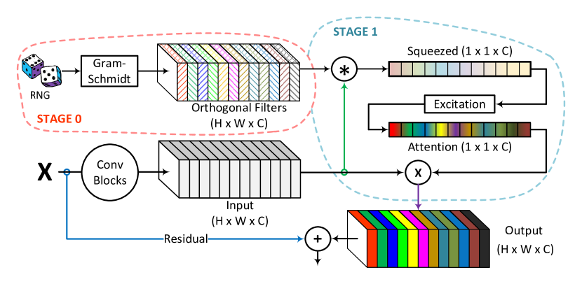
Figure 2: Illustration of orthogonal channel attention. Our method consists of two stages: Stage zero is initialization of random filters with sizes matching the feature layer sizes. We then use Gram-Schmidt process to make those filters orthonormal. Stage one utilizes those filters to extract the squeezed vector and use the excitation proposed by SENet to get the attention vector. By multiplying the attention vector with the input features, we calculate the weighted output features and add the residual.

III Method

In this section, we review the general formulation of channel attention mechanisms. With this formulation, we briefly review SENet and FcaNet. Based on these works, we introduce our method, Orthogonal Channel Attention, to be implemented in OrthoNet.

III-A Channel Attention

Considered a strongly influential attention mechanism, channel attention was first proposed in [11] as an add-on module to be incorporated into any existing architecture. Its goal is to improve overall network performance with negligible computational cost.

A channel attention block is a computational unit, built to encapsulate information and highlight relevant features. Suppose $X\in\mathbb{R}^{C}\times\mathbb{R}^{H}\times\mathbb{R}^{W}$ is a feature vector where $C$ is the number of channels with $H$ and $W$ being the height and width. The channel attention computes a vector, $A\in\mathbb{R}^{C}$, which highlights the most relevant channels of $X$. The output of the module is $A\odot X$, calculated by

$$(A\odot X)_{c,h,w}=A_{c}X_{c,h,w}\,.$$ (1)

Various researchers have proposed variants on Channel Attention that compute the attention vector, $A$, in different ways.

III-B Squeeze-and-Excitation (SENet)

The Squeeze-and-Excitation method is broken into two stages: a squeeze phase followed by an excitation stage. The squeeze stage can be considered a lossy-compression method using GAP as shown below:

$$Z_{c}=\mathbf{F}_{\text{se}}({X})_{c}=\frac{1}{HW}\sum_{i=1}^{H}\sum_{j=1}^{W}X_{c,i,j}\,.$$ (2)

The excite step maps the compressed descriptor $Z$ to a set of channel weights. This is achieved by

$$\mathbf{E}(Z)=\sigma(W_{2}\delta(W_{1}Z))\,,$$ (3)

where $\sigma$ is the sigmoid function, $\delta$ is the ReLU activation function, and $W_{1},W_{2}$ are (learnable) matrix weights. We can formulate channel attention in SENet in the following form:

$$A(X)=\mathbf{E}(\mathbf{F}_{\text{se}}(X))\,.$$ (4)

III-C Frequency Channel Attention (FcaNet)

One of the major weaknesses of the channel attention proposed in SENet [11] was the use of only one squeeze method: GAP. The authors were motivated to use GAP to encourage representation of global information in the attention vector. FcaNet [23] proposed an alternative squeeze method based on Discrete Cosine Transform. The DCT for an image of size $(H,W)$ with frequency component $(i,j)$ is given by

$$T_{i,j}(X)=\sum_{h=1}^{H}\sum_{w=1}^{W}v_{i}(h,H)v_{j}(w,W)X_{h,w}\,,$$ (5)

where

$$v_{k}(a,A)=\cos\left(\frac{\pi k(a+1/2)}{A}\right).$$ (6)

They proved that GAP is proportional to the initial DCT frequency, $(0,0)$, and demonstrated that the remaining frequencies need to be represented in the attention vector. They claim that those missing frequencies contain essential information; however, they give no theoretical reasoning to explain why their choice frequencies was optimal. FcaNet attention vector can be computed as follows:

$$A(X)=\mathbf{E}(\mathbf{F}_{\text{fca}}(X)),$$ (7)

where

$$\mathbf{F}_{\text{fca}}(X)_{c}=T_{I(c),J(c)}(X_{c})$$ (8)

for some choice of functions $I,J$ on the natural numbers. Based on experimental results, FcaNet chose to break the channel dimension into 16 blocks and chose $(I,J)$ to be constant on each block.

1

Input: Input Feature Dimension: $(C,H,W)$.

Output: Kernel $K\in\mathbb{R}^{C}\times\mathbb{R}^{H}\times\mathbb{R}^{W}$.

2 if $HW<C$ then

3       Calculate $n=\text{floor}(C/(HW))$

4       Initialize $\mathbf{L}$ as empty list

5       for $i\in\{0\dots n\}$ do

6             Initialize $HW$ random filters $F_{j}\in\mathbb{R}^{HW}$

7             Run Gram-Schmidt process on $\{F_{j}\}_{j=1}^{HW}$ to get an orthogonal set $\{F^{\prime}\}_{j=1}^{HW}$.

8             Append $\{F^{\prime}\}_{j=1}^{HW}$ to List $L$.

9            

10       end for

11      Concatenate filters in list $L$ to get kernel $K\in\mathbb{R}^{C}\times\mathbb{R}^{H}\times\mathbb{R}^{W}$.

12else

13       Initialize $C$ random filters $F_{j}\in\mathbb{R}^{HW}$

14       Run Gram-Schmidt process on $\{F_{j}\}_{j=1}^{C}$ to get an orthogonal set $\{F^{\prime}\}_{j=1}^{C}$.

15       Concatenate filters $\{F^{\prime}\}_{j=1}^{C}$ to get kernel $K\in\mathbb{R}^{C}\times\mathbb{R}^{H}\times\mathbb{R}^{W}$.

16 end if

17

Algorithm 1 Orthogonal Channel Attention Initialization (Stage Zero)

III-D Orthogonal Channel Attention (OrthoNet)

We notice that the DCTs used in FcaNet have a unique, essential, property: they are orthogonal [28]. In this paper, we exploit the benefits of the orthogonal property for channel attention. Roughly, we start by randomly selecting filters of the appropriate dimension, $(C,H,W)$; we then apply Gram-Schmidt process to make those filters orthonormal. The full details for initializing the filters are described in algorithm 1. Denoting these filters by $K\in\mathbb{R}^{C}\times\mathbb{R}^{H}\times\mathbb{R}^{W}$, our squeeze process is given by

$$\mathbf{F}_{\text{ortho}}(X)_{c}=\sum_{h=1}^{H}\sum_{w=1}^{W}K_{c,h,w}X_{c,h,w}\,.$$ (9)

As in the other methods, we define our channel attention by

$$A(X)=\mathbf{E}(\mathbf{F}_{\text{ortho}}(X))$$ (10)

TABLE I: Results of the image the classification task on ImageNet over different methods.

Method	Years	Backbone	Parameters	FLOPS	Train FPS	Test FPS	T1 acc	T5 acc
ResNet [9]	CVPR16	ResNet-34	21.80 M	3.68 G	2898	3840	74.58	92.05
SENet [11]	CVPR18		21.95 M	3.68 G	2729	3489	74.83	92.23
ECANet [33]	CVPR20		21.80 M	3.68 G	2703	3682	74.65	92.21
FcaNet-LF [23]	ICCV21		21.95 M	3.68 G	2717	3356	74.95	92.16
FcaNet-TS [23]	ICCV21		21.95 M	3.68 G	2717	3356	75.02	92.07
FcaNet-NAS [23]	ICCV21		21.95 M	3.68 G	2717	3356	74.97	92.34
WaveNet-C [25]	Bigdata22		21.95 M	3.68 G	2717	3356	75.06	92.376
OrthoNet+	CVPR22		21.95 M	3.68 G	2717	3356	75.22	92.5
ResNet [9]	CVPR16	ResNet-50	25.56 M	4.12 G	1644	3622	77.27	93.52
SENet [11]	CVPR18		28.07 M	4.13 G	1457	3417	77.86	93.87
CBAM [37]	ECCV18		28.07 M	4.14 G	1132	3319	78.24	93.81
GSoPNet1* [7]	CVPR19		28.29 M	6.41 G	1095	3029	79.01	94.35
GCNet [2]	ICCVW19		28.11 M	4.13 G	1477	3315	77.70	93.66
AANet [1]	ICCV19		25.80 M	4.15 G	-	-	77.70	93.80
ECANet [33]	CVPR20		25.56 M	4.13 G	1468	3435	77.99	93.85
FcaNet-LF [23]	ICCV21		28.07 M	4.13 G	1430	3331	78.43	94.15
FcaNet-TS [23]	ICCV21		28.07 M	4.13 G	1430	3331	78.57	94.10
FcaNet-NAS [23]	ICCV21		28.07 M	4.13 G		3331	78.46	94.09
OrthoNet+	CVPR22		28.07 M	4.13 G	1430	3331	78.47	94.12
OrthoNet-MOD+$	CVPR22		25.71 M	4.12 G	1430	3331	78.52	94.17
ResNet [9]	CVPR16	ResNet-101	44.55 M	7.85 G	816	3187	78.72	94.30
SENet [11]	CVPR18		49.29 M	7.86 G	716	2944	79.19	94.50
CBAM [37]	ECCV18		49.30 M	7.88 G	589	2492	78.49	94.31
AANet [1]	ICCV19		45.40 M	8.05 G	-	-	78.70	94.40
ECANet [33]	CVPR20		44.55 M	7.86 G	721	3000	79.09	94.38
FcaNet-LF[23]	ICCV21		49.29 M	7.86 G	705	2936	79.46	94.60
FcaNet-TS[23]	ICCV21		49.29 M	7.86 G	705	2936	79.63	94.63
FcaNet-NAS[23]	ICCV21		49.29 M	7.86 G	705	2936	79.53	94.64
OrthoNet+	CVPR22		49.29 M	7.86 G	705	2936	79.61	94.73
OrthoNet-MOD+$	CVPR22		44.84 M	7.85 G	705	2936	79.69	94.61

• * High computational cost. + Randomly initialized. $ Reduced number of parameters compared to SOTA.

IV Experimental Settings and Results

We begin by describing the details of our experiments. We then report the effectiveness of our method on image classification, object detection, and instance segmentation tasks.

IV-A Implementation Details

Following [11, 33, 23], we add our proposed attention module to ResNet-34 to construct OrthoNet-34. Based on ResNet-50 and 101, we construct two versions of our network called OrthoNet and OrthoNet-MOD. They differ in the position of the attention module in the ResNet blocks. For further details refer to section VI-B.

General Specifications

We adopt the Nvidia APEX mixed precision training toolkit and Nvidia DALI library for training efficiency. Our models are implemented in PyTorch [21], and are based on the code released by the authors of FcaNet [23]. The models were tested on two Nvidia Quadro RTX 8000 GPUs.

IV-A1 Classification

We utilize ImageNet [4], Places365 [44], and Birds [22] datasets to test and evaluate our method. To judge efficiency, we report the number of floating point operations per second (FLOPs) and the number of frames processed per second (FPS). To demonstrate method effectiveness, we report the top-1 and top-5 accuracies (T1, T5 acc). We use the same data augmentation and hyper-parameter settings found in [23]. Specifically, we apply random horizontal flipping, random cropping, and random aspect ratio. The resulting images are of size $256\times 256$.

During training, the SGD optimizer is set with a momentum of $0.9$, the learning rate is $0.2$, the weight decay is $1e-4$, and the batch size is $256$. All models are trained for $100$ epochs using Cosine Annealing Warm Restarts learning schedule and label smoothing. At the beginning of every tenth epoch, the learning rate scales by $10\%$ of the previous learning rate. Doing so fosters convergence, as demonstrated in [23].

IV-A2 Object Detection and Segmentation

We train and evaluate object detection and segmentation tasks using MS-COCO [17]. We report the average precision (AP) metric and its many variants.

FasterRCNN

We use FasterRCNN with OrthoNet-50 and 101 with one frozen stage and learnable BatchNorm. We use the same configuration used by FcaNet [23] based on MMDetection toolbox [3].

MaskRCNN

We use MaskRCNN with OrthoNet-50. We have one frozen stage and no learnable BatchNorm. We utilize the base configuration described in MMDetection toolbox [3] of ResNet-50.

Training Configuration

We train for 12 epochs. The SGD optimizer is set with a momentum of $0.9$. We warm up the model in the first 500 iterations starting with a learning rate of $1e-4$ and growing by $0.001$ every 50 iterations. After, we set the learning rate to $0.01$ for the first 8 epochs. At epoch 9, the learning rate decays to $0.001$ then at epoch 12 it decays to $0.0001$. We evaluate both FcaNet and our method using this configuration. For more details, refer to section VI-F.

IV-B Results

Classification Results

Accuracy results obtained on ImageNet are shown in I. The first noticeable feature is OrthoNet’s superior performance when using ResNet-34 as the backbone. The result shown in the table is an average over five trials with a standard deviation of $0.12$. Even in the worst case, we achieved $74.97$ which is comparable to FcaNet. Our results on ResNet-50 and 101 are better than both FcaNet-LF and FcaNet-NAS. The result for OrthoNet-50 is a mean over four trials with standard deviation of $0.07$.

The results obtained on ResNet-50 validate our initial hypothesis. If we Consider a linear scale with SENet mapping to zero and FcaNet mapping to one, our method achieves a $0.93$. Since SENet has the least orthogonal filters (they are all the same), this demonstrates the importance of orthogonal filters.

We believe that FcaNet slight improvement with ResNet-50 is because they choose particular filters that performed best on their experiments with ImageNet. To test this hypothesis, we evaluated our model on the Places365 and Birds classification datasets. Results are shown in II. We can see that our method outperforms FcaNet-TF on Birds by $0.18\%$ and on Places365 by $0.18\%$. These results imply that our method can generalize better to different datasets.

Object Detection Results

In addition to testing on ImageNet, Places365, and Birds datasets, we evaluate OrthoNet on MS COCO dataset to evaluate its performance on alternative tasks. We use OrthoNet and FPN [16] as the backbone of Faster R-CNN and Mask R-CNN.

As shown in Table III, when OrthoNet-MOD-50 is incorporated into the Faster-RCNN and Mask-RCNN frameworks performance surpasses that of FcaNet. We also achieve 10% less computational cost.

TABLE II: Results of Places365 dataset and Birds dataset. Our method achieves superior performance compared to FCANet. Both methods are trained using ResNet-50 backbone.

Method	Dataset	T1 acc	T5 acc
FcaNet-TS [23]	Places365 [44]	56.15	86.19
OrthoNet-MOD	Places365 [44]	56.33	86.18
FcaNet-TS [23]	Birds [22]	97.60	99.47
OrthoNet-MOD	Birds [22]	97.78	99.64

Segmentation Results

To further test our method, we evaluate OrthoNet-MOD-50 on instance segmentation task. As demonstrated in table IV, our method outperforms FcaNet under the ResNet-50 basic configuration of Mask-RCNN framework. These results verify the effectiveness of our method.

V Experimental Settings and Results

We begin by describing the details of our experiments. We then report the effectiveness of our method on image classification, object detection, and instance segmentation tasks.

V-A Implementation Details

Following [11, 33, 23], we add our proposed attention module to ResNet-34 to construct OrthoNet-34. Based on ResNet-50 and 101, we construct two versions of our network called OrthoNet and OrthoNet-MOD. They differ in the position of the attention module in the ResNet blocks. For further details refer to section VI-B.

V-A1 General Specifications

We adopt the Nvidia APEX mixed precision training toolkit and Nvidia DALI library for training efficiency. Our models are implemented in PyTorch [21], and are based on the code released by the authors of FcaNet [23]. The models were tested on two Nvidia Quadro RTX 8000 GPUs.

V-A2 Classification

We utilize ImageNet [4], Places365 [44], and Birds [22] datasets to test and evaluate our method. To judge efficiency, we report the number of floating point operations per second (FLOPs) and the number of frames processed per second (FPS). To demonstrate method effectiveness, we report the top-1 and top-5 accuracies (T1, T5 acc). We use the same data augmentation and hyper-parameter settings found in [23]. Specifically, we apply random horizontal flipping, random cropping, and random aspect ratio. The resulting images are of size $256\times 256$.

During training, the SGD optimizer is set with a momentum of $0.9$, the learning rate is $0.2$, the weight decay is $1e-4$, and the batch size is $256$. All models are trained for $100$ epochs using Cosine Annealing Warm Restarts learning schedule and label smoothing. At the beginning of every tenth epoch, the learning rate scales by $10\%$ of the previous learning rate. Doing so fosters convergence, as demonstrated in [23].

TABLE III: Results of the object detection task on COCO val 2017 over different methods.

Method	Detector	Parameters	FLOPs	AP	$AP_{50}$	$AP_{75}$	$AP_{S}$	$AP_{M}$	$AP_{L}$
ResNet-50	Faster-RCNN	41.53 M	215.51 G	36.4	58.2	39.2	21.8	40.0	46.2
SENet		44.02 M	215.63 G	37.7	60.1	40.9	22.9	41.9	48.2
ECANet		41.53 M	215.63 G	38.0	60.6	40.9	23.4	42.1	48.0
FcaNet-TS		44.02 M	215.63 G	39.0	61.1	42.3	23.7	42.8	49.6
OrthoNet-MOD		41.68 M	215.63 G	39.1	60.2	42.5	23.4	43.1	49.7
ResNet101	Faster-RCNN	60.52 M	295.39 G	38.7	60.6	41.9	22.7	43.2	50.4
SENet		65.24 M	295.58 G	39.6	62.0	43.1	23.7	44.0	51.4
ECANet		60.52 M	295.58 G	40.3	62.9	44.0	24.5	44.7	51.3
FcaNet-TS		65.24 M	295.58 G	41.2	63.3	44.6	23.8	45.2	53.1
OrthoNet-MOD		60.84 M	295.58 G	40.8	61.6	44.9	24.7	44.8	51.8
FcaNet-TS-50∗		46.66 M	261.93 G	37.3	57.5	40.5	22.1	40.4	48.2
OrthoNet-MOD∗	Mask-RCNN	44.53 M	261.93 G	37.8	57.9	41.1	22.5	41.3	48.2

• * Base configuration used for training. For more details refer to section V-A and section VI-F.

V-A3 Object Detection and Segmentation

We train and evaluate object detection and segmentation tasks using MS-COCO [17]. We report the average precision (AP) metric and its many variants.

FasterRCNN

We use FasterRCNN with OrthoNet-50 and 101 with one frozen stage and learnable BatchNorm. We use the same configuration used by FcaNet [23] based on MMDetection toolbox [3].

MaskRCNN

We use MaskRCNN with OrthoNet-50. We have one frozen stage and no learnable BatchNorm. We utilize the base configuration described in MMDetection toolbox [3] of ResNet-50.

V-A4 Training Configuration

We train for 12 epochs. The SGD optimizer is set with a momentum of $0.9$. We warm up the model in the first 500 iterations starting with a learning rate of $1e-4$ and growing by $0.001$ every 50 iterations. After, we set the learning rate to $0.01$ for the first 8 epochs. At epoch 9, the learning rate decays to $0.001$ then at epoch 12 it decays to $0.0001$. We evaluate both FcaNet and our method using this configuration. For more details, refer to section VI-F.

V-B Results

Classification Results

Accuracy results obtained on ImageNet are shown in I. The first noticeable feature is OrthoNet’s superior performance when using ResNet-34 as the backbone. The result shown in the table is an average over five trials with a standard deviation of $0.12$. Even in the worst case, we achieved $74.97$ which is comparable to FcaNet. Our results on ResNet-50 and 101 are better than both FcaNet-LF and FcaNet-NAS. The result for OrthoNet-50 is a mean over four trials with standard deviation of $0.07$.

The results obtained on ResNet-50 validate our initial hypothesis. If we Consider a linear scale with SENet mapping to zero and FcaNet mapping to one, our method achieves a $0.93$. Since SENet has the least orthogonal filters (they are all the same), this demonstrates the importance of orthogonal filters.

We believe that FcaNet slight improvement with ResNet-50 is because they choose particular filters that performed best on their experiments with ImageNet. To test this hypothesis, we evaluated our model on the Places365 and Birds classification datasets. Results are shown in II. We can see that our method outperforms FcaNet-TF on Birds by $0.18\%$ and on Places365 by $0.18\%$. These results imply that our method can generalize better to different datasets.

TABLE IV: Results of the instance segmentation task on COCO val 2017 over different methods using Mask R-CNN.

Method	AP	AP50	AP75	APS	APM
FcaNet-TS-50	34.0	54.6	36.1	18.5	37.1
OrthoNet-MOD	34.4	55.0	36.8	19.0	37.5

• Base configuration used for training. For more details refer to

• section V-A and section VI-F.

Object Detection Results

In addition to testing on ImageNet, Places365, and Birds datasets, we evaluate OrthoNet on MS COCO dataset to evaluate its performance on alternative tasks. We use OrthoNet and FPN [16] as the backbone of Faster R-CNN and Mask R-CNN.

As shown in Table III, when OrthoNet-MOD-50 is incorporated into the Faster-RCNN and Mask-RCNN frameworks performance surpasses that of FcaNet. We also achieve 10% less computational cost.

Segmentation Results

To further test our method, we evaluate OrthoNet-MOD-50 on instance segmentation task. As demonstrated in table IV, our method outperforms FcaNet under the ResNet-50 basic configuration of Mask-RCNN framework. These results verify the effectiveness of our method.

VI Discussion

We begin with a possible explanation for the success of OrthoNet. We then detail our explorations into variants of our architecture and conclude by discussing implementation and limitations.

VI-A Potential Mechanism for Our Success

While FcaNet believes that frequency choice for the discrete cosine transform is the primary factor for a successful attention mechanism, our results imply that the key driving force behind successful attention mechanisms is distinct (orthogonal) attention filters. In brief, we believe that the success of FcaNet is mostly due to the orthogonality of the DCT kernels.

Recall that convolutional neural networks contain built-in redundancy [45, 10, 23] (i.e., hidden features with strongly correlated channel slices). In a standard SENet, the squeeze method will extract the same information from these redundant channels. In fact, by appropriately permuting the learnable parameters of a SENet, one can construct another network where the only difference is the order of the channels in the intermediate features. (Such a trick cannot be applied to FcaNet and OrthoNet due to the presence of constant, orthogonal squeeze filters.) The existence of this permutation method implies that SENet cannot, a priori, prescribe meaning to its channels.

When the filters are orthogonal, the information they extract comes from orthogonal subspaces of the feature space ($\mathbb{R}^{H}\times\mathbb{R}^{W}$). Hence, they focus distinct characteristics. Since the gradient information flows backward through the network, the convolutional kernels preceding the squeeze can adapt to their unique mapping. By doing so, the network can extract a richer representation for every feature map, which the excitation can then build upon.

To further support our ideas, we train OrthoNet-34 and 50 using random filters — we omit the Gram-Schmidt step — and obtain accuracies of $74.63$ and $76.77$ respectively. We can clearly see the effect of orthogonal filters on improving the validation accuracy on both networks compared to random filter and GAP (Table I).

VI-B Attention Module Location

The overall structure of a ResNet-50 or 101 bottleneck block is shown in figure 3. To construct OrthoNet, we follow the standard procedure placing the attention module following the $1\times 1$ convolution. Motivated by the below reasoning, we moved the attention in those networks to follow the $3\times 3$ convolution. The resulting network is OrthoNet-MOD.

In OrthoNet-34, the attention is placed on the second $3\times 3$ convolution in each block. We now recall the structure of ResNet 50 and 101: both networks contains many blocks consisting of a $1\times 1$ convolution followed by a $3\times 3$ convolution then another $1\times 1$ convolution (with batch-norms and activations placed between). Since the $1\times 1$ convolutions can only consider inter-channel relationships and lack the ability to capture spatial information, they are mainly used for feature refinement and for channel resizing. Combined with an activation, a $1\times 1$ convolution can be considered as a Convolutional MLP [15]. Since the $3\times 3$ convolutions are the only modules that consider spatial-relationships, they must extract rich spacial information if the network hopes to achieve high accuracies. These motivations and the success of OrthoNet-34 lead to the construction of OrthoNet-MOD.

This modification yields many benefits. First, we reduce the number of parameters used for the attention module by only creating filters of the same size as we did in OrthoNet-34. Exact parameter counts can be found in Table I. Second, we improve accuracies over the standard OrthoNet. Third, we place the attention at a more meaningful location, the $3\times 3$ convolution, where features are richer in spacial information.

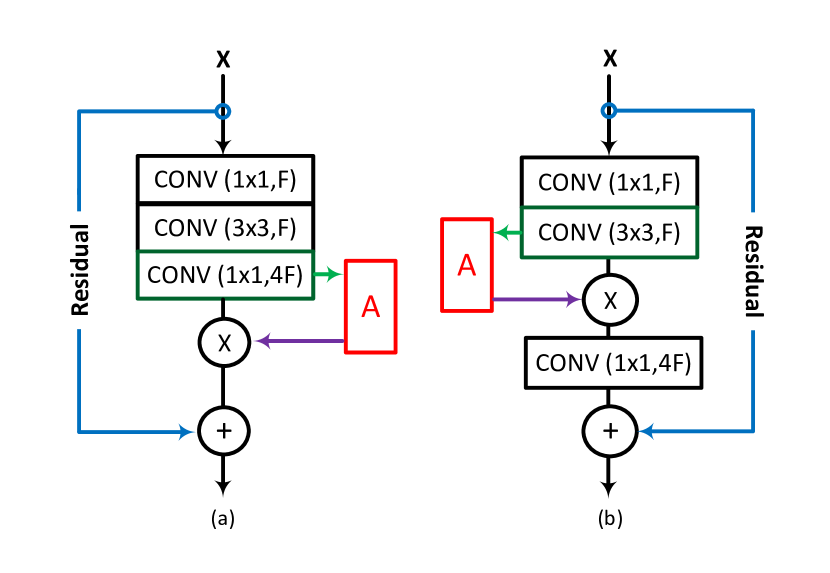
Figure 3: (a) OrthoNet block vs (b) OrthoNet-MOD block

VI-C Cross-talk Effect on Orthogonal Filters

Our squeeze method can be considered as a convolution with kernel size equal to the feature spacial dimensions and groups equal to the number of channels — group size equal to one. Since increasing group size allows inter-communication between channels; one might hypothesize that doing so could allow the squeeze step to extract richer representations of the input feature. To investigate such a hypothesis on OrthoNet, we conduct experiments using OrthoNet-34 with different grouping sizes. The results are recorded in Table V. The results indicate that the group size is inconsequential; however, due to time and computational constraints, we were only able to run each experiment once, and more experiments need to be conducted.

TABLE V: Effect of Grouping.

Method				Group Size			Top-1 acc
OrthoNet-34				1			75.13
				4			75.20
				$H\times W$			75.18

VI-D Fine-Tuning channel attention filters

In this section, we experiment with allowing the orthogonal filters to learn and fine-tune. We implement multiple different learning methods. First, we train OrthoNet-34 on constant orthogonal filters, then introduce learning the filters in the last twenty epochs. We call this method FineTuned-20. Second, we implement FineTuned-40, where we learn during each epoch that’s divisible by five and also for the last twenty epochs — 40 epochs in total. Third, we implement learning the first 30 epochs — FineTuned-30 — then we disable learning the filters and continue training for the remaining 70 epochs on OrthoNet-50. Experiments demonstrate that learning the filters for OrthoNet-MOD-50 doesn’t improve the overall validation accuracy. As for OrthoNet-34, we observe a more consistent accuracies for different learning methods. Results are shown in table VI. Further investigation is needed on the method of training and the potential inclusion of an attention-specific loss function for optimal learning.

TABLE VI: Effect of Squeeze Filter Learning.

Backbone	Learning Method	Top-1 acc
OrthoNet-34	FineTuned-20	75.20
OrthoNet-34	FineTuned-40	75.24
OrthoNet-50	FineTuned-40	78.50
OrthoNet-MOD-50	FineTuned-40	78.30
OrthoNet-MOD-50	FineTuned-30	78.36

VI-E Ease of Integration

Similar to SENet and FcaNet, our module can easily be integrated to any existing convolutional networks. The major distinction between SENet, FcaNet and our method is the adoption of different channel compression methods. As discussed earlier, our method can be described as a convolution as shown in 1 and can be implemented with a single line of code.

VI-F Limitations

Random filters have a natural limitation. In upper layers, where $HW>C$, it is impossible to have filters that comprise a full basis (i.e., you must choose $C$ filters from the $HW$ total). Although we did not observe it, a poor choice of filters may exist. Their unlearnable nature makes this a persistent factor throughout training. This could lead to a failure case. However; in the lower layers, we are able — and do — create a complete basis for $\mathbb{R}^{HW}$ which eliminates this issue in those layers.

Although we reported the means for OrthoNet-34 over five trials and OrthoNet-50 over four trials; due to limitations in time and computational capabilities, we only ran most other experiments once. Due to the limited number of runs, we could not report the standard deviation. However, OrthoNet’s constant higher accuracy on a variety of tasks and datasets suggest the robustness of our network.

For the object detection and segmentation with MaskRCNN, we utilize the base configuration provided by MMDetection [3]. The results reported by the base configuration are different from those of their configuration. We were unable to use the configuration used by FcaNet [23] because of technical difficulties.

We also used the results of the experiments conducted by FcaNet for previous methods (FasterRCNN and ImageNet); however, we conducted our experiments under the same configuration.

VII Conclusion

In this work, we introduced a variant of SENet which utilizes orthogonal squeeze filters to create an effective channel attention module that can be integrated into any existing network. To evaluate its performance, we constructed OrthoNet and demonstrated state-of-the-art performance on Birds, Places365, and COCO with competitive or superior performance on ImageNet. By comparing OrthoNet to state-of-the-art, we’ve found that the key driving force to a successful attention mechanism is orthogonal attention filters. Orthogonal filters allow for maximum information extraction from any correlated features and allow the network to prescribe meaning to each channel yielding a more effective attention squeeze.

Our future works include further investigating learnable orthogonal filters, implementing metrics for evaluation of attention mechanisms, and further pruning our attention module to lower the computational cost and improve our method accuracy. We’re also searching for a theoretical framework to explain the channel attention phenomenon.

References

- [1] Irwan Bello, Barret Zoph, Ashish Vaswani, Jonathon Shlens, and Quoc V. Le. Attention augmented convolutional networks. In Proceedings of the IEEE/CVF International Conference on Computer Vision (ICCV), October 2019.
- [2] Yue Cao, Jiarui Xu, Stephen Lin, Fangyun Wei, and Han Hu. Gcnet: Non-local networks meet squeeze-excitation networks and beyond, 2019.
- [3] K Chen, J Wang, J Pang, Y Cao, Y Xiong, X Li, S Sun, W Feng, Z Liu, J Xu, et al. Mmdetection: Open mmlab detection toolbox and benchmark. arxiv 2019. arXiv preprint arXiv:1906.07155.
- [4] J. Deng, W. Dong, R. Socher, L.-J. Li, K. Li, and L. Fei-Fei. ImageNet: A Large-Scale Hierarchical Image Database. In CVPR09, 2009.
- [5] Jun Fu, Jing Liu, Haijie Tian, Yong Li, Yongjun Bao, Zhiwei Fang, and Hanqing Lu. Dual attention network for scene segmentation, 2018.
- [6] Hiroshi Fukui, Tsubasa Hirakawa, Takayoshi Yamashita, and Hironobu Fujiyoshi. Attention branch network: Learning of attention mechanism for visual explanation. In Proceedings of the IEEE/CVF Conference on Computer Vision and Pattern Recognition (CVPR), June 2019.
- [7] Zilin Gao, Jiangtao Xie, Qilong Wang, and Peihua Li. Global second-order pooling convolutional networks, 2018.
- [8] Kaiming He, Georgia Gkioxari, Piotr Dollar, and Ross Girshick. Mask r-cnn. In Proceedings of the IEEE International Conference on Computer Vision (ICCV), Oct 2017.
- [9] Kaiming He, Xiangyu Zhang, Shaoqing Ren, and Jian Sun. Deep residual learning for image recognition. In Proceedings of the IEEE Conference on Computer Vision and Pattern Recognition (CVPR), June 2016.
- [10] Yihui He, Xiangyu Zhang, and Jian Sun. Channel pruning for accelerating very deep neural networks. In Proceedings of the IEEE international conference on computer vision, pages 1389–1397, 2017.
- [11] Jie Hu, Li Shen, and Gang Sun. Squeeze-and-excitation networks. In 2018 IEEE/CVF Conference on Computer Vision and Pattern Recognition, pages 7132–7141, 2018.
- [12] Gao Huang, Zhuang Liu, Laurens van der Maaten, and Kilian Q. Weinberger. Densely connected convolutional networks, 2016.
- [13] Alex Krizhevsky, Ilya Sutskever, and Geoffrey E Hinton. Imagenet classification with deep convolutional neural networks. In F. Pereira, C.J. Burges, L. Bottou, and K.Q. Weinberger, editors, Advances in Neural Information Processing Systems, volume 25. Curran Associates, Inc., 2012.
- [14] Yann LeCun, Léon Bottou, Yoshua Bengio, and Patrick Haffner. Gradient-based learning applied to document recognition. In Proceedings of the IEEE, volume 86, pages 2278–2324, 1998.
- [15] Min Lin, Qiang Chen, and Shuicheng Yan. Network in network. arXiv preprint arXiv:1312.4400, 2013.
- [16] Tsung-Yi Lin, Piotr Dollár, Ross Girshick, Kaiming He, Bharath Hariharan, and Serge Belongie. Feature pyramid networks for object detection. In 2017 IEEE Conference on Computer Vision and Pattern Recognition (CVPR), pages 936–944, 2017.
- [17] Tsung-Yi Lin, Michael Maire, Serge Belongie, Lubomir Bourdev, Ross Girshick, James Hays, Pietro Perona, Deva Ramanan, C. Lawrence Zitnick, and Piotr Dollár. Microsoft coco: Common objects in context, 2014.
- [18] Shuying Liu and Weihong Deng. Very deep convolutional neural network based image classification using small training sample size. In 2015 3rd IAPR Asian Conference on Pattern Recognition (ACPR), pages 730–734, 2015.
- [19] Diganta Misra, Trikay Nalamada, Ajay Uppili Arasanipalai, and Qibin Hou. Rotate to attend: Convolutional triplet attention module, 2020.
- [20] Xuran Pan, Chunjiang Ge, Rui Lu, Shiji Song, Guanfu Chen, Zeyi Huang, and Gao Huang. On the integration of self-attention and convolution. In Proceedings of the IEEE/CVF Conference on Computer Vision and Pattern Recognition (CVPR), pages 815–825, June 2022.
- [21] Adam Paszke, Sam Gross, Francisco Massa, Adam Lerer, James Bradbury, Gregory Chanan, Trevor Killeen, Zeming Lin, Natalia Gimelshein, Luca Antiga, Alban Desmaison, Andreas Köpf, Edward Yang, Zach DeVito, Martin Raison, Alykhan Tejani, Sasank Chilamkurthy, Benoit Steiner, Lu Fang, Junjie Bai, and Soumith Chintala. Pytorch: An imperative style, high-performance deep learning library, 2019.
- [22] Gerald Piosenka. Birds 450 - species image classification. 02 2022.
- [23] Zequn Qin, Pengyi Zhang, Fei Wu, and Xi Li. Fcanet: Frequency channel attention networks. In Proceedings of the IEEE/CVF International Conference on Computer Vision (ICCV), pages 783–792, October 2021.
- [24] Shaoqing Ren, Kaiming He, Ross Girshick, and Jian Sun. Faster r-cnn: Towards real-time object detection with region proposal networks. In C. Cortes, N. Lawrence, D. Lee, M. Sugiyama, and R. Garnett, editors, Advances in Neural Information Processing Systems, volume 28. Curran Associates, Inc., 2015.
- [25] Hadi Salman, Caleb Parks, Shi Yin Hong, and Justin Zhan. Wavenets: Wavelet channel attention networks, 2022.
- [26] Xibin Song, Yuchao Dai, Dingfu Zhou, Liu Liu, Wei Li, Hongdong Li, and Ruigang Yang. Channel attention based iterative residual learning for depth map super-resolution. In IEEE/CVF Conference on Computer Vision and Pattern Recognition (CVPR), June 2020.
- [27] Rupesh Kumar Srivastava, Klaus Greff, and Jürgen Schmidhuber. Highway networks, 2015.
- [28] Gilbert Strang. The discrete cosine transform. SIAM Review, 41(1):135–147, 1999.
- [29] Christian Szegedy, Wei Liu, Yangqing Jia, Pierre Sermanet, Scott Reed, Dragomir Anguelov, Dumitru Erhan, Vincent Vanhoucke, and Andrew Rabinovich. Going deeper with convolutions. In 2015 IEEE Conference on Computer Vision and Pattern Recognition (CVPR), pages 1–9, 2015.
- [30] Hao Tang, Dan Xu, Nicu Sebe, Yanzhi Wang, Jason J. Corso, and Yan Yan. Multi-channel attention selection gan with cascaded semantic guidance for cross-view image translation. In Proceedings of the IEEE/CVF Conference on Computer Vision and Pattern Recognition (CVPR), June 2019.
- [31] Hugo Touvron, Andrea Vedaldi, Matthijs Douze, and Herve Jegou. Fixing the train-test resolution discrepancy. In H. Wallach, H. Larochelle, A. Beygelzimer, F. d'Alché-Buc, E. Fox, and R. Garnett, editors, Advances in Neural Information Processing Systems, volume 32. Curran Associates, Inc., 2019.
- [32] Vibashan VS, Vikram Gupta, Poojan Oza, Vishwanath A. Sindagi, and Vishal M. Patel. Mega-cda: Memory guided attention for category-aware unsupervised domain adaptive object detection. In Proceedings of the IEEE/CVF Conference on Computer Vision and Pattern Recognition (CVPR), pages 4516–4526, June 2021.
- [33] Qilong Wang, Banggu Wu, Pengfei Zhu, Peihua Li, Wangmeng Zuo, and Qinghua Hu. Eca-net: Efficient channel attention for deep convolutional neural networks, 2019.
- [34] Wenguan Wang, Shuyang Zhao, Jianbing Shen, Steven C. H. Hoi, and Ali Borji. Salient object detection with pyramid attention and salient edges. In Proceedings of the IEEE/CVF Conference on Computer Vision and Pattern Recognition (CVPR), June 2019.
- [35] Xiaolong Wang, Ross Girshick, Abhinav Gupta, and Kaiming He. Non-local neural networks, 2017.
- [36] Xudong Wang, Long Lian, and Stella X. Yu. Unsupervised visual attention and invariance for reinforcement learning. In Proceedings of the IEEE/CVF Conference on Computer Vision and Pattern Recognition (CVPR), pages 6677–6687, June 2021.
- [37] Sanghyun Woo, Jongchan Park, Joon-Young Lee, and In So Kweon. Cbam: Convolutional block attention module, 2018.
- [38] Zhuofan Xia, Xuran Pan, Shiji Song, Li Erran Li, and Gao Huang. Vision transformer with deformable attention. In Proceedings of the IEEE/CVF Conference on Computer Vision and Pattern Recognition (CVPR), pages 4794–4803, June 2022.
- [39] Saining Xie, Ross Girshick, Piotr Dollar, Zhuowen Tu, and Kaiming He. Aggregated residual transformations for deep neural networks. In Proceedings of the IEEE Conference on Computer Vision and Pattern Recognition (CVPR), July 2017.
- [40] Sergey Zagoruyko and Nikos Komodakis. Wide residual networks, 2016.
- [41] Matthew D. Zeiler and Rob Fergus. Visualizing and understanding convolutional networks. In David Fleet, Tomas Pajdla, Bernt Schiele, and Tinne Tuytelaars, editors, Computer Vision – ECCV 2014, pages 818–833, Cham, 2014. Springer International Publishing.
- [42] Ting Zhao and Xiangqian Wu. Pyramid feature attention network for saliency detection. In Proceedings of the IEEE/CVF Conference on Computer Vision and Pattern Recognition (CVPR), June 2019.
- [43] Zilong Zhong, Zhong Qiu Lin, Rene Bidart, Xiaodan Hu, Ibrahim Ben Daya, Zhifeng Li, Wei-Shi Zheng, Jonathan Li, and Alexander Wong. Squeeze-and-attention networks for semantic segmentation. In IEEE/CVF Conference on Computer Vision and Pattern Recognition (CVPR), June 2020.
- [44] Bolei Zhou, Agata Lapedriza, Aditya Khosla, Aude Oliva, and Antonio Torralba. Places: A 10 million image database for scene recognition. IEEE Transactions on Pattern Analysis and Machine Intelligence, 2017.
- [45] Zhuangwei Zhuang, Mingkui Tan, Bohan Zhuang, Jing Liu, Yong Guo, Qingyao Wu, Junzhou Huang, and Jinhui Zhu. Discrimination-aware channel pruning for deep neural networks. Advances in neural information processing systems, 31, 2018.