Analytical approximations of Lotka-Volterra integrals

Abstract

In this note we derive simple analytical approximations for the solutions of $x-\log x=y-\log y$ and use them for estimating trajectories following Lotka-Volterra-type integrals. We show how our analytical approximations imply estimates for trajectories of general predator-prey systems, including e.g. Rosenzweig McArthur equations.

2010 Mathematics Subject Classification. Primary 34D23, 34C05.

Keywords: Rosenzweig McArthur; Predator prey; Size of limit cycle; Lyapunov

1 Introduction

Consider the Lotka-Volterra system

$$\frac{dS}{dt}=aS-bSX,$$

$$\frac{dX}{dt}=cSX-dX,$$

where $S=S(t)$ represents prey and $X=X(t)$ predator biomass, and $a$, $b$, $c$ and $d$ are positive constants. By introducing the nondimensional quantities $x(\tau)=\frac{b}{a}X(t),\,s(\tau)=\frac{c}{d}S(t),\,\tau=at,\,\alpha=\frac{d}{a}$ we obtain the equivalent system

$$\frac{ds}{d\tau}=(1-x)s,$$

$$\frac{dx}{d\tau}=\alpha x(s-1),$$ (1.1)

which, by the corresponding phase-plane equation, has its trajectories on level curves of

$$V(x,s)=\frac{1}{\alpha}\left(x-\ln x\right)+s-\ln s.$$ (1.2)

In this note we derive analytical bounds for solutions of the Lotka-Volterra integral (1.2). Indeed, we prove that the solution $x<1$ of the equation $x-\ln(x)=y-\ln(y)$, where $y>1$, satisfies the relation $x=zY$, where $Y=ye^{-y}$ and $1<z<e$ and $z=z(y)$ is a decreasing function of $y$. We also prove that the inequalities $1<z_{1}<z<z_{2}<z_{0}<e$, where the $z_{i}$s are explicit functions of $Y$, hold for $z$, see Theorem 2.1 in Section 2.

To apply the theorem, consider a trajectory $T$ of system (1) with initial condition $(x_{0},s_{0})$ with $s_{0}>1$. If we aim for an estimate of the $s$-value for the next intersection of $T$ with the line $x=x_{0}$ at, say $(x_{0},s_{1})$, then we intend to estimate the solution of $V(x_{0},s_{0})=V(x_{0},s_{1})$, i.e. the solution $s_{1}<1<s_{0}$ of

$$s_{1}-\ln s_{1}=s_{0}-\ln s_{0}.$$

According to the theorem we find

$$s_{1}=z(s_{0})s_{0}e^{-s_{0}}$$

in which the function $z$ is decreasing and can be estimated so that

$$1<z_{1}<\frac{s_{1}}{s_{0}}e^{s_{0}}<z_{2}<z_{0}<e$$ (1.3)

where $z_{i}=z_{i}(s_{0})$, $i=0,1,2$. Likewise, if trajectory $T$ starts at $(x_{0},s_{0})$ with $x_{0}>1$, then we may find an estimate of the next intersection of $T$ with the line $s=s_{0}$ through the equation $V(x_{0},s_{0})=V(x_{1},s_{0})$, which boils down to $x_{1}-\ln x_{1}=x_{0}-\ln x_{0}$. As above we conclude, for the solution $x_{1}<1<x_{0}$,

$$1<z_{1}<\frac{x_{1}}{x_{0}}e^{x_{0}}<z_{2}<z_{0}<e$$ (1.4)

where $z_{i}=z_{i}(x_{0})$, $i=0,1,2$. Observe that any level of predator or prey can be chosen, giving estimates for the next intersection of the trajectory at the same predator or prey level. For example, if we wish to estimate the minimal predator biomass, $x_{\text{min}}$, on a trajectory having maximal predator biomass $x_{\text{max}}$, then we use the fact that both maximal and minimal predator biomass are attained on the isocline $x^{\prime}=0$, i.e. at the prey biomass $s_{0}=1$. From (1.4) we obtain

$$1<z_{1}<\frac{x_{\text{min}}}{x_{\text{max}}}e^{x_{\text{max}}}<z_{2}<z_{0}<e$$

where $z_{i}=z_{i}(x_{\text{max}})$, $i=0,1,2$. Clearly, we can obtain the similar estimates for $s_{\text{min}}$ as function of $s_{\text{max}}$ using (1.3) and $x_{0}=1$. Figure 1 shows the estimates for $s_{1}$ in (1.3) with $(x_{0},s_{0})=(2,2)$, and the estimates for $x_{1}$ in (1.4) with $(x_{0},s_{0})=(2,1/2)$.

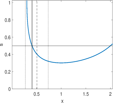
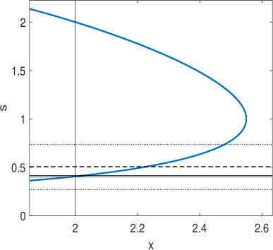
Figure 1: The estimates of trajectory $T$ by $z_{1}$ and $z_{2}$ (solid), $z_{0}$ (dashed) and $1$ and $e$ (dotted). Estimates for $s$ in (1.3) with $(x_{0},s_{0})=(2,2)$ (Left panel), and for $x$ in (1.4) with $(x_{0},s_{0})=(2,1/2)$ (Right panel). Here, $\alpha=1$.

A literature survey shows extensive interest in analysing Lotka-Voltera-type systems and their generalizations. To mention a few, we refer the reader to [10, 2, 3, 5] and the references therein. Estimates valid for small prey biomass such as (1.3) may be of importance when studying the predators hunting strategies, e.g., if there is a threshold of the prey level at which the predator chose to switch from their central prey and instead starts to feed on other sources. We give further motivations and demonstrations on how our theorem can be used to derive estimates of trajectories to more general dynamical systems in Section 3. In the next section, we present the theorem and its proof.

2 The theorem

In this section we prove the following analytical estimates:

Theorem 2.1

The solution $x<1$ to the equation $x-\ln(x)=y-\ln(y)$, where $y>1$ satisfies the relation $x=z\,Y$, where $Y=y\,e^{-y}$ and $1<z<e$ and $z=z(y)$ is decreasing in $y$.

Moreover, let $d_{i}=e-1-c_{i}\,e$, $c_{0}=0$, $c_{1}=\frac{e-2}{e-1}$, $c_{2}=\frac{1}{e}$, for $i=0,1,2$, $Y=y\,e^{-y}$ and

$$z_{i}(y)=\frac{1-d_{i}\,Y-\sqrt{(1-d_{i}\,Y)^{2}-4c_{i}\,Y}}{2c_{i}\,Y},\quad i=1,2,\quad\text{and}\quad z_{0}(y)=\frac{1}{1-(e-1)Y}.$$

Then, the inequalities $1<z_{1}<z<z_{2}<z_{0}<e$ hold for $z$.

A numerical solution of the equation in Theorem 2.1 and the three approximations are plotted in Figure 2. Before giving the proof we remark that any equation of type $x-a\,\ln(x)=y-a\,\ln(y)\,0<x<a<y$ can be transformed into the equation of Theorem 2.1 by scaling $x$ and $y$.

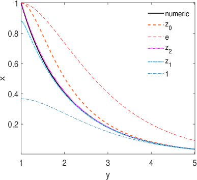
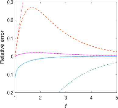
Figure 2: Left panel: Approximations to the solution of the equation $x-\log x=y-\log y$ in Theorem 2.1. The black solid curve gives a numerical solution for $x$ as a function of $y$. The green dashdot curve corresponds to the lower bound determined by $z_{1}$, the magenta dotted curve to upper bound by $z_{2}$ while the read dashed curve corresponds to upper bound determined by $z_{0}$. Right panel: Relative error.

Proof of Theorem 2.1. We begin by proving the first statement of the Theorem by substituting $x=z\,Y$ into the equation of the theorem to obtain

$$Z(z)=Y\quad\text{in which}\quad Z(z)=\frac{\ln(z)}{z}.$$ (2.5)

This equation has a unique solution for $z$, where $1<z<e$, because $0<Y<1/e$ for $y>1$ and $Z$ is increasing in $z$ and $Z(1)=0$ and $Z(e)=1/e$. Derivation of formula (2.5) with respect to $y$ gives $z^{\prime}=z^{2}\,e^{-y}\,\frac{y-1}{x-1}<0$ and $z$ is decreasing in $y$.

In order to get the estimates for $z$ we let

$$f_{i}(z)=\frac{z-1}{c_{i}\,z+d_{i}}.$$

The proof is based on the inequalities

$$f_{0}(z)<f_{2}(z)<\ln z<f_{1}(z)\quad\text{for}\quad 1<z<e.$$ (2.6)

We denote by $z^{*}$ the solution to equation (2.5). Then $Z(z)<Y$ for $z<z^{*}$ and $Z(z)>Y$ for $z>z^{*}$. Thus if $Y=\frac{f_{i}(z_{i})}{z_{i}}<Z(z_{i})$ then $z^{*}<z_{i}$ and if $Y=\frac{f_{i}(z_{i})}{z_{i}}>Z(z_{i})$ then $z^{*}>z_{i}$. In order to prove (2.6) we now consider the functions $g_{i}$ defined by

$$g_{i}(z)=\ln z-f_{i}(z).$$

Calculating the derivative of $g_{i}$ we get

$$g_{i}^{\prime}(z)=\frac{h_{i}(z)}{z\,(c_{i}\,z+d_{i})^{2}}\quad\text{in which}\quad h_{i}(z)=c_{i}^{2}\,z^{2}+(2d_{i}\,c_{i}-c_{i}-d_{i})\,z+d_{i}^{2}.$$

We notice that $h_{1}$ is negative between 1 and $\frac{1}{(e-2)^{2}}$, positive between $\frac{1}{(e-2)^{2}}$ and $e$, and because $g(1)=g(e)=0$, we conclude that $g_{1}(z)<0$ between 1 and $e$. Thus $\frac{f_{1}(z)}{z}>Z(z)$ and because $z_{1}$ is the solution to $\frac{f_{1}(z)}{z}=Y$ we get $z^{*}>z_{1}$.

Further, $h_{2}$ is positive between 1 and $e\,(e-2)^{2}$, negative between $e\,(e-2)^{2}$ and $e$ and because $g(1)=g(e)=0$, we conclude that $g_{2}(z)>0$ between 1 and $e$. Thus $\frac{f_{2}(z)}{z}<Z(z)$ and because $z_{2}$ is the solution to $\frac{f_{2}(z)}{z}=Y$ we get $z^{*}<z_{2}$.

Finally, $h_{0}$ is positive between 1 and $e-1$, negative between $e-1$ and $e$ and because $g(1)=g(e)=0$, we conclude that $g_{0}(z)>0$ between 1 and $e$. Thus $\frac{f_{0}(z)}{z}<Z(z)$ and because $z_{0}$ is the solution to $\frac{f_{0}(z)}{z}=Y$ we get $z^{*}<z_{0}$. $\hfill\Box$

3 Applications to more general systems

Consider a general predator-prey system on the form

$$S^{\prime} =H(S)-q\varphi(S)X,$$

$$X^{\prime} =p\varphi(S)X-dX,$$ (3.7)

where the non-negative variable $S$ represents the prey biomass, the non-negative variable $X$ represents the predator biomass, $\varphi$ is non-decreasing, $\varphi(0)=H(0)=0$, and parameters $p,q,d$ are positive. Systems of type (3) have been extensively studied through the last centuries, see e.g. [1, 6, 7, 4, 8, 9] and the references therein.

Often, functions $H$ and $\varphi$ are defined by

$$H(S)=rS\left(1-\frac{S}{K}\right)\quad\text{and}\quad\varphi(S)=\frac{S^{n}}{S^{n}+A},$$ (3.8)

where most commonly $n=1$ or $n=2$. In case of (3.8) system (3) is usually referred to as a Rosenzweig-MacArthur predator prey system. If

$$H(S)=rS\quad\text{and}\quad\varphi(S)=S,$$

then system (3) boils down to the Lotka-Volterra equations (1).

We now intend to analyze the general system (3) using our estimates in Theorem 2.1. Assume, without loss of generality, that $q=1$. The phase-plane equation yields

$$\frac{dS}{dX}=\frac{F(S)-X}{X}\cdot\frac{\varphi(S)}{p\varphi(S)-d}$$

where $F(S)=H(S)/\varphi(S)$. Let us replace $F(S)$ by a constant $\overline{F}$ for the moment, and observe that then integrating gives

$$\int\left(p-\frac{d}{\varphi(S)}\right)dS=\int\left(\frac{{\overline{F}}}{X}-1\right)dX$$

and thus the system can, under reasonable assumptions on $\varphi$ and $H$, be analyzed by the generalized Lotka-Volterra integral

$$V(X,S)=pS-d\int\frac{dS}{\varphi(S)}+X-{\overline{F}}\log{X}.$$

Moreover

$$\nabla V=\left(1-\frac{\overline{F}}{X},p-\frac{d}{\varphi(S)}\right)$$ (3.9)

and

$$\frac{\partial V}{\partial t} =\left(p-\frac{d}{\varphi(S)}\right)S^{\prime}+\left(1-\frac{\overline{F}}{X}\right)X^{\prime}=\left(p\varphi(S)-d\right)\left(F(S)-{\overline{F}}\right).$$ (3.10)

Suppose that we are in a part of the state space where there exist positive $\underline{F}$ and $\overline{F}$ such that

$$\underline{F}<F(S)<\overline{F}\quad\text{and}\quad\varphi(S)<d/p.$$ (3.11)

It then follows from (3.9) and (3.10) that a trajectory $T$ starting at $(X_{0},S_{0})$ remains trapped between the curves $\underline{S}$ and $\overline{S}$, defined through

$$V_{\underline{F}}(X_{0},S_{0})=V_{\underline{F}}(X,\underline{S}(X))\quad\text{and}\quad V_{\overline{F}}(X_{0},S_{0})=V_{\overline{F}}(X,\overline{S}(X)),$$

see Figure 3.

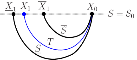
Figure 3: Geometry in the construction of estimates.

Moreover, the ‘barriers’ $\underline{S}$ and $\overline{S}$ are convex with min at $X=\underline{F}$ and $X=\overline{F}$, and intersect $S=S_{0}$ a second time at $\underline{X}_{1}$ and $\overline{X}_{1}$, respectively. For the next intersection of $T$ with $S=S_{0}$ at $(X_{1},S_{0})$ it necessarily holds that

$$\underline{X}_{1}<X_{1}<\overline{X}_{1},$$

where

$$V_{\underline{F}}(X_{0},S_{0})=V_{\underline{F}}(\underline{X}_{1},S_{0})\quad\text{giving}\quad X_{0}-\underline{F}\log{X_{0}}=\underline{X}_{1}-\underline{F}\log{\underline{X}_{1}},$$

and

$$V_{\overline{F}}(X_{0},S_{0})=V_{\overline{F}}(\overline{X}_{1},S_{0})\quad\text{giving}\quad X_{0}-\overline{F}\log{X_{0}}=\overline{X}_{1}-\overline{F}\log{\overline{X}_{1}}.$$

By setting $x=\frac{\underline{X}_{1}}{\underline{F}}$ and $y=\frac{X_{0}}{\underline{F}}$ the first equation reads

$$x-\ln(x)=y-\ln(y),$$

and by assuming $y=\frac{X_{0}}{\underline{F}}>1$ an application of Theorem 2.1 gives

$$x=z\left(y\right)ye^{-y},$$

where $z$ is a decreasing function of $y$. As the same argument applies to the upper barrier we conclude

$$z\left(\frac{X_{0}}{\underline{F}}\right){X_{0}}e^{-\frac{X_{0}}{\underline{F}}}=\underline{X}_{1}<X_{1}<\overline{X}_{1}=z\left(\frac{X_{0}}{\overline{F}}\right){X_{0}}e^{-\frac{X_{0}}{\overline{F}}}.$$

Finally, applying Theorem 2.1 for estimating $z$ yields

$$e^{-\frac{X_{0}}{\underline{F}}}<z_{1}e^{-\frac{X_{0}}{\underline{F}}}<\frac{X_{1}}{X_{0}}<z_{2}e^{-\frac{X_{0}}{\overline{F}}}<z_{0}e^{\frac{X_{0}}{\overline{F}}}<e^{1+\frac{X_{0}}{\overline{F}}},$$ (3.12)

where $z_{1}=z_{1}\left(\frac{X_{0}}{\underline{F}}\right)$, $z_{2}=z_{2}\left(\frac{X_{0}}{\overline{F}}\right)$ and $z_{0}=z_{0}\left(\frac{X_{0}}{\overline{F}}\right)$. As a remark, we note that the accuracy of (3.12) improves when $F(S)=H(S)/\varphi(S)$ obeys less variation, i.e., when one can take a tighter interval in assumption (3.11).

As an example, for which we easily find the above imposed assumptions satisfied and thereby conclude (3.12), we consider the system

$$s^{\prime} =(h(s)-x)s$$

$$x^{\prime} =m\,(s-\lambda)\,x$$ (3.13)

in $x,s\geq 0$, supposing parameters $m,\,\lambda>0$, $\lambda<1$ and where $h$ is given by

$$h(s)=(1-s)(s+a).$$ (3.14)

Any standard Rosenzweig-McArthur predator-prey system can be transformed into a system of type (3). In particular, it is equivalent with system (3) when (3.8) holds with $n=1$, which can be seen by introducing the non-dimensional quantities

$$\tau\,=\,\int\frac{rK}{H+S\left(t\right)}dt,\quad s \,=\,\frac{S}{K},\quad x\,=\,\frac{qX}{rK},\quad a\,=\,\frac{H}{K},$$

$$m\,=\,\frac{p-d}{r}\quad \text{and}\quad\lambda\,=\,\frac{dH}{(p-d)K}.$$ (3.15)

Comparing to the general system (3) we identify $S=s,X=x,F(S)=h(s),\varphi(S)=s,p=m$, and $d=m\lambda$. Hence, since $a<h(s)=(1-s)(s+a)<h(\lambda)$ when $s<\lambda$, we obtain (3.11) satisfied in the region $s<\lambda$ with $\underline{F}=a$ and $\overline{F}=h(\lambda)$. Observing that $s=\lambda$ is the isocline $x^{\prime}=0$ we conclude, from (3.12), the following estimate for the minimal predator biomass, $x_{\text{min}}$:

$$e^{-\frac{x_{\text{max}}}{a}}<z_{1}e^{-\frac{x_{\text{max}}}{a}}<\frac{x_{\text{min}}}{x_{\text{max}}}<z_{2}e^{-\frac{x_{\text{max}}}{h(\lambda)}}<z_{0}e^{\frac{x_{\text{max}}}{h(\lambda)}}<e^{1+\frac{x_{\text{max}}}{h(\lambda)}},$$ (3.16)

where $z_{1}=z_{1}\left(\frac{x_{\text{max}}}{a}\right)$, $z_{2}=z_{2}\left(\frac{x_{\text{max}}}{h(\lambda)}\right)$ and $z_{0}=z_{0}\left(\frac{x_{\text{max}}}{h(\lambda)}\right)$.

We remark that by shrinking the region $s<\lambda$ into $s<\lambda^{*}$ for some $0<\lambda^{*}<\lambda$ we have the better estimates $a<h(s)<h(\lambda^{*})$ and may, for a trajectory starting at $(x_{0},\lambda^{*})$, estimate its next intersection with the line $s=\lambda^{*}$ at point $(x_{1},\lambda^{*})$. In particular, we then get (3.16) but with $x_{\text{max}}=x_{0}$, $x_{\text{min}}=x_{1}$ and $h(\lambda)=h(\lambda^{*})$. Furthermore, we observe that the upper estimate is good for small $\lambda^{*}$ but becomes less efficient when the value of $\lambda$ increases beyond $a$. The bounds in (3.16) will be used by the authors in [9] for estimating the size of the unique limit cycle to system (3) which is the global attractor when $2\lambda+a<1$.

Two predators

As a final remark we consider the following system similar to (3) but allowing for $n\geq 1$ predators:

$$S^{\prime} =H(S)-\sum_{i=1}^{n}q_{i}\varphi_{i}(S)X_{i},$$

$$X_{i}^{\prime} =p_{i}\varphi_{i}(S)X_{i}-d_{i}X_{i},$$ (3.17)

where the non-negative variable $S$ represents the prey biomass, the non-negative variables $X_{i}$ represent the predator biomasses, $\varphi_{i}$ is non-decreasing, $\varphi(0)=H(0)=0$, parameters $p_{i}$, $q_{i}$, $d_{i}$ are positive. Assuming $p_{i}>d_{i}$ and using a time change and a variable change (similar to (3)) we can, when

$$H(S)=rS\left(1-\frac{S}{K}\right)\quad\text{and}\quad\varphi_{i}(S)=\frac{S}{S+A_{i}},$$

transform system (3) to the system

$$s^{\prime} =\left(1-s-\sum_{i=1}^{n}\frac{x_{i}}{s+a_{i}}\right)s,$$

$$x_{i}^{\prime} =m_{i}\frac{s-\lambda_{i}}{s+a_{i}}x_{i}.$$

Here the new variables are normalized biomasses $x_{i}$ and $s$ and the parameters are positive. Systems of this type have been studied e.g. in [11, 12, 13].

Suppose $\lambda_{1}>\lambda_{2}$. If

$$a_{2}>\frac{a_{1}}{L+a_{1}(L-1)}\quad\text{and}\quad L=\frac{\lambda_{1}(1-\lambda_{2})}{\lambda_{2}(1-\lambda_{1})},$$

the predator corresponding to $x_{1}$ goes extinct. In opposite case there can be coexistence or one of predators go extinct. For $\lambda_{2}>\lambda_{1}$ there is a symmetric result where the predator corresponding to $x_{2}$ goes extinct, see [11, 13] and references therein. The proof considered only behaviour of functions $\varphi_{i}$ and thus there are possibilities for improving the results. We observe that if one of $x_{i}$ is zero we get a two-dimensional system of the types considered in previous sections. Often these systems have limit cycles and the stability or instability of these cycles are important for understanding the extinction or coexistence possibilities for the predators. It occurs that the behaviour for small prey biomass on the cycle can play an important role in determining the stability, see [13] and references therein, and thus estimates of the limit cycle for small prey, such as (3.12), obtained by Theorem 2.1, may be useful.

References

- [1] Cheng K.-S. Uniqueness of a limit cycle for a predator-prey system. SIAM Journal on Mathematical Analysis 12.4 (1981): 541-548.
- [2] Clanet C., Villermaux E. An analytical estimate of the period for the delayed logistic application and the Lotka-Volterra system. The European Physical Journal B-Condensed Matter and Complex Systems, 6 (1998): 529-536.
- [3] Grozdanovski T., Shepherd J. Approximating the periodic solutions of the Lotka-Volterra system. ANZIAM Journal, 49 (2007): C243-C257.
- [4] Hsu, S.-B., Shi, J.: Relaxation oscillator profile of limit cycle in predator-prey system. Discrete and continuous dynamical systems B 11, no. 4 (2009): 893-911.
- [5] Ito H. C., Dieckmann U., Metz J. A. Lotka-Volterra approximations for evolutionary trait-substitution processes. Journal of Mathematical Biology, 80(7) (2020): 2141-2226.
- [6] Lindström T. A generalized uniqueness theorem for limit cycles in a predator-prey system. Acta Academiae Aboensis, Series B: Mathematica et Physica, 49(2) (1989).
- [7] Lindström T. Why do rodent populations fluctuate?: stability and bifurcation analysis of some discrete and continuous predator-prey models Doctoral dissertation, Luleå tekniska universitet (1994).
- [8] Lundström N L P, Söderbacka G, Estimates of size of cycle in a predator-prey system, Differential Equations and Dynamical Systems, 2018, DOI: 10.1007/s12591-018-0422-x
- [9] Lundström N L P, Söderbacka G, Estimates of size of cycle in a predator-prey system II, Preprint
- [10] Murty K. N., Rao D. V. G. Approximate analytical solutions of general Lotka-Volterra equations. J. Math. Anal. Applic., 122(2) (1987): 582-588.
- [11] Osipov A V, Söderbacka G, Extinction and coexistence of predators. Dinamicheskie Sistemy, 6, 1 (2016): 55-64.
- [12] Osipov A V, Söderbacka G, Poincaré map construction for some classic two predators-one prey systems. Internat. J. Bifur. Chaos Appl. Sci. Engrg,27, (8) (2017): 1750116, 9 pp.
- [13] Osipov A V, Söderbacka G, Review of results on a system of type many predators-one prey. Nonlinear Systems and Their Remarkable Mathematical Structures (2018): 520-540. CRC Press.