Grouping Local Process Models

Abstract

In recent years, process mining emerged as a proven technology to analyze and improve operational processes. An expanding range of organizations using process mining in their daily operation brings a broader spectrum of processes to be analyzed. Some of these processes are highly unstructured, making it difficult for traditional process discovery approaches to discover a start-to-end model describing the entire process. Therefore, the subdiscipline of Local Process Model (LPM) discovery tries to build a set of LPMs, i.e., smaller models that explain sub-behaviors of the process. However, like other pattern mining approaches, LPM discovery algorithms also face the problems of model explosion and model repetition, i.e., the algorithms may create hundreds if not thousands of models, and subsets of them are close in structure or behavior. This work proposes a three-step pipeline for grouping similar LPMs using various process model similarity measures. We demonstrate the usefulness of grouping through a real-life case study, and analyze the impact of different measures, the gravity of repetition in the discovered LPMs, and how it improves after grouping on multiple real event logs.

1 Introduction

Process mining is a scientific discipline for discovering, monitoring, and improving processes via readily-available data from different data management systems. The three main pillars of process mining are process discovery, conformance checking, and process enhancement [1]. As the interest in process mining grows, new applications pose new challenges. One such challenge is discovering a single start-to-end model for highly unstructured processes ([19, Figure 7]). To resolve this problem, one usually focuses on frequent behavior because of the $80/20$ rule of data variability. However, in some domains, especially ones covering human behavior, the rule does not hold and better solutions are needed. A relatively new field is Local Process Model (LPM) discovery [19], where the idea is to build smaller process models explaining fragments of the behavior instead of one overall model. Yet, current LPM discovery approaches return hundreds or thousands of models for one event log (model explosion), with highly similar models repeating between them (model repetition) as shown in Figure 1. Although this is desirable in some use cases [7, 14], it does not help with a better understanding of highly variable processes.

To alleviate this problem, in this work, we propose a pipeline that groups similar LPMs, and for each group, one representative LPM is chosen. By doing so, highly similar models that describe small differences in behavior are grouped together, allowing analysts to focus on the bigger picture by examining a smaller diverse set of LPMs and only dive deeper into the differences when necessary. More specifically, we start with an LPM discovery approach that returns a set of LPMs. These LPMs are then clustered such that model similarity, using different process model similarity measures, is measured, and for each cluster, a representative LPM is chosen. We evaluate the proposed approach on multiple event logs by comparing model diversity between the originally returned set of LPMs and the representative set obtained after grouping. Additionally, we demonstrate the benefit of clustering LPMs by inspecting a smaller set of models on the BPIC2012-res10939 event log.

((a)) Three highest ranked LPMs discovered by [19].

((b)) Three highest ranked LPMs discovered by [16].

Figure 1: LPMs discovered using [19] and [16] on the filtered and transformed BPIC2012 event log for resource $10939$ as explained in [19].

The rest of the paper is structured as follows. In Section 2, we introduce the needed preliminaries to follow the rest of the paper. Section 3 introduces what LPMs are and in Section 4 we present different process model similarity measures. We explain the framework in Section 5 and we present the obtained results in Section 6. We conclude the paper with final remarks in Section 7.

2 Preliminaries

2.1 General

We define sets ($X=\{a,b\}$), multisets ($M=[a^{2},b^{3}]$), sequences ($\sigma=\langle a,b,c\rangle$), and tuples ($t=(a,b,c)$) as usual. Given a set $X$, $\mathcal{P}(X)$ is the power set of $X$, $X^{*}$ represents the set of all sequences over $X$, and $\mathbb{M}(X)$ is the set of all multisets over $X$. We use $\sigma(i)$ to denote the $i$-th element of the sequence $\sigma$ and $M(a)=2$ to denote that item $a$ appears twice in the multiset $M$.

We use $f(X)=\{f(x)|x\in X\}$ (and $f(\sigma)=\langle f(\sigma(1)),f(\sigma(2)),...,f(\sigma(n))\rangle$) to apply the function $f$ to every element in the set $X$ (the sequence $\sigma$) and $f_{\upharpoonright_{X}}$ (respectively $\sigma_{\upharpoonright_{X}}$) to denote the projection of the function $f$ (respectively the sequence $\sigma$) on the set $X$.

2.2 Process Mining

Normally, the collected data used for process analysis is transformed in the form of event logs. Hence, in Definition 1, we formally define traces and event logs. Note that although traces are usually defined as sequences of events, in this work, we are only interested in the activity executed by each event.

Definition 1 (Trace, Event Log)

Given the universe of activities $\mathcal{A}$, we define $\rho\in\mathcal{A}^{*}$ as a trace, and $L\in\mathbb{M}(\mathcal{A}^{*})$ as an event log.

In Definition 2, we define labeled Petri nets. Note that a transition $t\in T$ with $l(t)=\tau$ is called silent and that there may be duplicate transitions $t_{1},t_{2}\in T$ such that $l(t_{1})=l(t_{2})$.

Definition 2 (Labeled Petri net)

A labeled Petri net $N=(P,T,F,l)$ is a tuple, where $P$ is a set of places and $T$ is a set of transitions such that $P\cap T=\emptyset$. $F\subseteq(P\times T)\cup(T\times P)$ is the flow relation, and $l:T\to\mathcal{A}\cup\{\tau\}$ the labeling function.

Now, given a node $x\in P\cup T$, we define the preset of $x$ as $\bullet x=\{y\in P\cup T|(y,x)\in F\}$ and the postset of $x$ as $x\bullet=\{y\in P\cup T|(x,y)\in F\}$.

To attach behavior to labeled Petri nets we use a marking and the firing rule. A marking $M$ denotes the state of a Petri net as a multiset of places ($M\in\mathbb{M}(P)$) and the firing rule allows for changes between states (i.e., markings). Given a marking $M$, a transition $t$ is enabled in the marking $M$ if and only if $\bullet t\subseteq M$. If a transition $t$ is enabled in the marking $M$, it can fire and change the state of the net to a new marking $M^{\prime}=(M\setminus\bullet t)\cup t\bullet$. We write $M\xrightarrow{t}M^{\prime}$. A sequence of transitions $\sigma=\langle t_{1},\dots,t_{n}\rangle\in T^{*}$ is enabled in $M$ and by firing it marking $M^{\prime}$ is reached if and only if there exist $M_{0}$, $M_{1}$, $\dots$, $M_{n}$ such that $M_{0}=M$, $M_{n}=M^{\prime}$, and $M_{i-1}\xrightarrow{t_{i}}M_{i}$ for $1\leq i\leq n$. We write $M\xrightarrow{\sigma}M^{\prime}$.

Now, we formally define an accepting Petri net in Definition 3 and the set of all its firing sequences in Definition 4.

Definition 3 (Accepting Labeled Petri Net)

An accepting labeled Petri net is a triple $(N,M_{i},M_{f})$ such that $N=(P,T,F,l)$ is a labeled Petri net, $M_{i}\in\mathbb{M}(P)$ is the initial marking, and $M_{f}\in\mathbb{M}(P)$ is the final marking.

Definition 4 (Complete Firing Sequences)

Let $\textrm{AN}=(N,M_{i},M_{f})$ be an accepting Petri net, $\mathcal{F}(\textrm{AN})=\{\sigma\in T^{*}|M_{i}\xrightarrow{\sigma}M_{f}\}$ is the set of complete firing sequences for AN.

3 Local Process Models

In contrast to process discovery, whose task is to discover one model that explains the traces of an event log from start to end, LPM discovery tries to mine a set of models each matching some particular sub-behavior represented by subsequences in the event log.

LPMs were first introduced in [19] as a replacement for process discovery of highly unstructured processes. However, afterward, the use cases where LPMs are used expanded (e.g., [6, 7, 10, 12, 13, 14, 17]) and multiple approaches and extensions for LPM discovery followed [3, 16, 5].

All existing approaches [3, 16, 19], with the exception of [5], suffer from the model explosion problem. The approach in [5] first finds common subsequences and then discovers models on them. This, however, makes it predisposed to similar problems as the traditional process discovery approaches and restricts the set of LPMs use-case scenarios the approach can be applied to. Still, as everyone else, they are prone to the model repetition problem. The approach in [19] incrementally extends process trees by adding new nodes, in [3] two existing LPMs (represented with process trees) differing only in one node are joined together to create a larger LPM. In the new model, the differing nodes are added as children to one of the process tree operators. Finally, in [16], LPMs are created by joining place nets together. This makes it clear that all approaches would build highly similar, i.e., repetitive models. Additionally, if one focuses on frequent behavior, the highly similar models would all explain highly similar behavior making highly-ranked models contain clusters of repetitive models. The implementations of [19] and [16] offer a rudimentary grouping of the models. However, it becomes evident this is not sufficient when one considers human analysts manually inspecting and analyzing hundred of LPMs. Therefore, with this work, we try to alleviate this shortcoming of LPM discovery approaches.

In this work, we focus on LPMs discovered with [16]. Therefore, although LPMs can, in general, be represented by any modeling language (Petri nets, process trees, BPMNs, etc.), in this work we restrict to a subclass of accepting labeled Petri nets. We show a few example LPMs in Figure 1(b) and we give a formal definition in Definition 5. We use $T_{in}=\{t\in T|\bullet t=\emptyset\}$ to denote the transitions that have an empty preset and we call them unrestricted transitions. We define the set of complete valid firing sequences of such LPMs in Definition 6 by restricting that each place in the net can receive at most one token from unrestricted transitions.

Definition 5 (Local Process Models)

A Local Process Model (LPM) is an accepting labeled Petri net $\textit{lpm}=(N_{\textit{lpm}},M_{i},M_{f})$ such that $N_{\textit{lpm}}=(P,T,F,l)$ is a labeled Petri net that satisfies the following restrictions:

1. $\forall_{x,x^{\prime}\in P\cup T}\,\exists_{\langle x_{1},\dots,x_{n}\rangle}(x=x_{1}\land x^{\prime}=x_{n}\land\forall_{1\leq i<n}((x_{i},x_{i+1})\in F)\lor(x_{i+1},x_{i})\in F))$, i.e., there is only one connected component, and

2. $\forall_{p\in P}(\bullet p\neq\emptyset\land p\bullet\neq\emptyset)$, i.e., each place has at least one incoming and one outgoing arc,

and $M_{i}\in\mathbb{M}(P)$ and $M_{f}\in\mathbb{M}(P)$ are the initial and final marking. We use $\mathbb{U}_{\textit{LPM}}$ to denote the universe of such LPMs.

Definition 6 (Local Process Model Behavior)

Given an LPM $\textit{lpm}=(N_{\textit{lpm}},M_{i},M_{f})$ such that $N_{\textit{lpm}}=(P,T,F,l)$, we define $\mathcal{F}_{\textit{LPM}}(\textit{lpm})=\{\sigma\in\mathcal{F}(\textit{lpm})|\forall_{1\leq i<j\leq|\sigma|}(\sigma(i)\in T_{in}\land\sigma(j)\in T_{in}\implies\sigma(i)\bullet\cap\sigma(j)\bullet=\emptyset)\}$ to be all valid complete firing sequences of lpm.

The language of an LPM lpm is obtained by projecting all valid complete firing sequences on the transition labels and removing $\tau$-skips, i.e., $\mathcal{L}(\textit{lpm})=\{l(\sigma)_{\upharpoonright_{\mathcal{A}}}|\sigma\in\mathcal{F}_{\textit{LPM}}(\textit{lpm})\}$. We use $\mathcal{L}^{n}(\textit{lpm})=\{l(\sigma)_{\upharpoonright_{\mathcal{A}}}|\sigma\in\mathcal{F}_{\textit{LPM}}(\textit{lpm})\land|\sigma|\leq n\}$ to denote the language restricting to complete firing sequences of length at most $n$. We can use the language to measure conformance with respect to an event log $L$ and rank the LPMs. The ranking can take into consideration different quality measures, such as fitness, precision, and simplicity. We write $\textit{rank}_{L}\in\mathbb{U}_{\textit{LPM}}\not\to\mathbb{N}$ to denote a ranking function, and $\mathbb{U}_{\textit{rank}}$ to denote the universe of all such ranking functions.

We later use these definitions to extract features from the LPMs and formalize the different similarity measures.

4 Process Model Similarity Measures

To get an overview of existing similarity measures, we considered multiple survey papers [8, 9, 18, 20, 4]. Although there can be small differences in how they categorize different similarity measures, all of them agree, the basic split is into measures that compare the structure of the process model and those that compare the behavior. Subsequently, one can consider the level of abstraction used, e.g., complete language versus weak order relations. Therefore, we choose five representative similarity measures. Before introducing the specific measures, we first define what a similarity measure is in Definition 7.

Definition 7 (Similarity Measure)

A similarity measure $\mathit{sim}_{\mathit{name}}\in\mathbb{U}_{\textit{LPM}}\times\mathbb{U}_{\textit{LPM}}\to[0,1]$ is a function that calculates the similarity between two LPMs. We use $`\mathit{name}`$ to distinguish a specific measure, and $\mathbb{U}_{sim}$ to denote the universe of all similarity measures.

To introduce the similarity measures, we assume we are given two LPMs $\textit{lpm}_{A}=(N^{A}_{\textit{lpm}},[\hskip 1.00006pt\hskip 1.00006pt],[\hskip 1.00006pt\hskip 1.00006pt])$ s.t. $N^{A}_{\textit{lpm}}=(P_{A},T_{A},F_{A},l_{A})$ and $\textit{lpm}_{B}=(N^{B}_{\textit{lpm}},[\hskip 1.00006pt\hskip 1.00006pt],[\hskip 1.00006pt\hskip 1.00006pt])$ s.t. $N^{B}_{\textit{lpm}}=(P_{B},T_{B},F_{B},l_{B})$. In the following, we illustrate the measures we use in this work with the help of $\textit{lpm}_{A}$ and $\textit{lpm}_{B}$.

Transition label comparison is the most simple measure we investigate. The measure calculates the transition label overlap between the models.

$$\mathit{sim}_{\textit{transition}}(\textit{lpm}_{A},\textit{lpm}_{B})=\frac{2*|l_{A}(T_{A})\cap l_{B}(T_{B})|}{|l_{A}(T_{A})|+|l_{B}(T_{B})|}$$

Node comparison is somewhat more complex, in that it includes place overlap as well. We use this measure to represent structural measures using abstraction. The measure calculates the similarity between two models by combining transition label comparison and place matching between the nets. We assign to each pair of places a matching gain $g(p_{1},p_{2})=\frac{1}{2}*\frac{2*|l_{A}(\bullet p_{1})\cap l_{B}(\bullet p_{2})|}{|l_{A}(\bullet p_{1})|+|l_{B}(\bullet p_{2})|}+\frac{1}{2}*\frac{2*|l_{A}(p_{1}\bullet)\cap l_{B}(p_{2}\bullet)|}{|l_{A}(p_{1}\bullet)|+|l_{B}(p_{2}\bullet)|}$ and we use the Hungarian algorithm [11] to solve the assignment problem. We use $G_{\textit{places}}$ to represent the gain of the optimal assignment. Then, we define the measure as

$$\mathit{sim}_{\textit{node}}(\textit{lpm}_{A},\textit{lpm}_{B})=\frac{2*|l_{A}(T_{A})\cap l_{B}(T_{B})|+2*G_{\textit{places}}}{|l_{A}(T_{A})|+|l_{B}(T_{B})|+|P_{A}|+|P_{B}|}$$

Eventually-follow graph similarity is a behavioral abstraction measure that measures the overlap of the eventually-follows relation in the languages of the two models. We calculate it as

$$\mathit{sim}_{\textit{efg}}^{n}(\textit{lpm}_{A},\textit{lpm}_{B})=\frac{2*|\textit{EF}^{\,n}_{A}\cap\textit{EF}^{\,n}_{B}|}{|\textit{EF}^{\,n}_{A}|+|\textit{EF}^{\,n}_{B}|}$$

such that $\textit{EF}_{A}^{\,n}=\{(a,b)|\exists_{\rho\in\mathcal{L}^{n}(\textit{lpm}_{A})}(\exists_{1\leq i<j\leq|\rho|}(a=\rho_{i}\land b=\rho_{j}))\}$ and $\textit{EF}^{\,n}_{B}$ is defined correspondingly.

Full trace matching comparison represents the more sophisticated behavioral measures. We define it as

$$sim^{n}_{\textit{full}}(\textit{lpm}_{A},\textit{lpm}_{B})=\frac{2*G_{\textit{traces}}}{|\mathcal{L}^{n}(\textit{lpm}_{A})|+|\mathcal{L}^{n}(\textit{lpm}_{B})|}$$

where $G_{\textit{traces}}$ represents the gain of the optimal trace assignment. To calculate the gain between two traces we invert the normalized Levenshtein distance.

Finally graph edit model comparison represents sophisticated structural measures. It calculates model similarity by using the graph edit distance (ged) as defined in [2], where the node substitution cost is $1$ if the nodes differ in type, i.e., one is a place and the other transitions, or if the compared nodes are differently labeled transitions. The node substitution cost between two places is calculated as $1-g(p_{1},p_{2})$, where $g(p_{1},p_{2})$ is the gain defined as before. The edge substitution cost takes the average of the node substitution cost between the source and sink nodes of the two edges. To convert the ged to a similarity measure, we use the formula below.

$$sim_{\textit{ged}}(\textit{lpm}_{A},\textit{lpm}_{B})=1-ged(\textit{lpm}_{A},\textit{lpm}_{B})$$

In the remainder, we also use the term distance measure, which we always consider to be the inverse of the similarity, i.e., $\textit{dist}_{\textit{name}}(\textit{lpm}_{A},\textit{lpm}_{B})=1-\mathit{sim}_{\textit{name}}(\textit{lpm}_{A},\textit{lpm}_{B})$ for any $\textit{name}\in\{\textit{transition},\textit{node},\textit{efg},\textit{full},\textit{ged}\}$

5 Method to Group LPMs

In this work, we propose a three-step pipeline that starts with an event log and a multitude of process model comparison measures and ends with groups of similar LPMs, as shown in Figure 2. The first step is discovering LPMs (Step $1$), which can also be omitted, starting the pipeline with a set of LPMs instead. Then, the models are clustered such that the similarity between them is determined by the previously defined process model similarity measures (Step $2$). Finally, for each cluster, we choose a representative model (Step $3$).

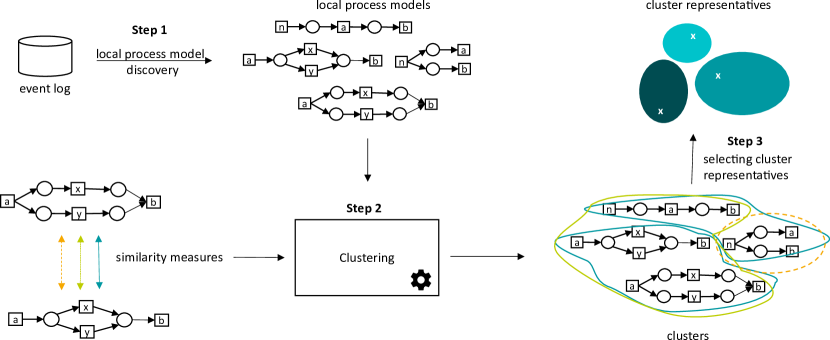
Figure 2: Illustration of the proposed three-step pipeline.

5.1 Local Process Model Discovery (Step 1)

In the first step, we focus on discovering a set of LPMs $\textit{LPM}_{L}$ given an event log $L$. Although multiple approaches are available, in this work, we use the approach presented in [16]. The produced models are ranked from highest to lowest using a rank function $\textit{rank}_{L}$ as previously defined.

5.2 Clustering (Step 2)

In the clustering step, we accept a set of LPMs and a similarity measure and return a set of clusters. We define the universe of LPM cluster sets in Definition 8, and a clustering algorithm in Definition 9.

Definition 8 (Universe of Local Process Model Cluster Sets)

We define $\mathbb{U}_{\sqcap}=\{X_{\textit{LPM}}\subseteq\mathcal{P}(\textit{LPM}_{L})|\textit{LPM}_{L}\subseteq\mathbb{U}_{\textit{LPM}}\land\emptyset\not\in X_{\textit{LPM}}\land\bigcup X_{\textit{LPM}}=\textit{LPM}_{L}\}$ to be the universe of LPM cluster sets.

Definition 9 (Clustering Algorithm)

We define $\textit{clust}\in\mathcal{P}(\mathbb{U}_{\textit{LPM}})\times\mathbb{U}_{sim}\not\to\mathbb{U}_{\sqcap}$ to be a clustering algorithm. To denote a clustering algorithm given some set of parameters $P$, we write $\textit{clust}_{P}$.

The goal of the clustering algorithm is to return the LPMs in homogeneous groups, such that the similarity is high within the individual groups and low between them. One clustering algorithm can produce different cluster sets for the same model set based on the parameters $P$. In our work, we focus on hierarchical clustering and consider distance threshold and linkage as possible parameters. In particular, we use linkage to determine how the distance between two clusters containing multiple models is calculated and the distance threshold to determine the maximum merging distance. For the traditional hierarchical clustering algorithm, we use the returned clusters in $\sqcap_{\textit{LPM}_{L}}=\textit{clust}_{P}(\textit{LPM}_{L},sim_{\textit{name}})$ for an LPM set $\textit{LPM}_{L}$ discovered on an event log $L$ and a similarity measure $sim_{\textit{name}}$ are pairwise disjoint, i.e., $\forall_{\textit{LPM}_{i},\textit{LPM}_{j}\in\sqcap_{\textit{LPM}_{L}}}\textit{LPM}_{i}\cap\textit{LPM}_{j}=\emptyset$. We overload the notation $\sqcap_{\textit{LPM}_{L}}(\textit{lpm})$ to denote the cluster in the cluster set $\sqcap_{\textit{LPM}_{L}}$ in which the LPM lpm belongs. That is, it holds $\textit{lpm}\in\sqcap_{\textit{LPM}_{L}}(\textit{lpm})\in\sqcap_{\textit{LPM}_{L}}$.

5.3 Choosing Cluster Representatives (Step 3)

In Step 3, we take a set of LPMs $\textit{LPM}_{L}\subseteq\mathbb{U}_{\textit{LPM}}$ discovered on an event log $L$ in Step 1, and a computed cluster set $\sqcap_{\textit{LPM}_{L}}=\textit{clust}(\textit{LPM}_{L},sim_{\textit{name}})$ from Step 2. We return an LPM set $\sqcap_{\textit{LPM}_{L}}^{\textit{repr}}$ in which we keep only one representative LPM per cluster. In this work, we choose representative models either by taking the highest-ranked LPM in each cluster considering some ranking function $\textit{rank}_{L}\in\mathbb{U}_{\textit{rank}}$ or the LPM with the minimal mean distance to all other LPMs in the cluster. In Definition 10, we formally define representative projection as a function that maps a set of LPMs to one model.

Definition 10 (Representative projection)

A representative projection $\textit{repr}\in\mathcal{P}(\mathbb{U}_{\textit{LPM}})\not\to\mathbb{U}_{\textit{LPM}}$ is a function that takes an LPM set $\textit{LPM}_{L}$ and returns one representative LPM. We use $\textit{repr}_{\textit{rank}}$ and $\textit{repr}_{\textit{dist}}$ to denote the representation projections based on the highest ranking and minimal mean distance respectively.

Now, for the set of LPMs $\textit{LPM}_{L}\subseteq\mathbb{U}_{\textit{LPM}}$, we create the set $\sqcap_{\textit{LPM}_{L}}^{\textit{repr}_{x}}=\{\textit{repr}_{x}(\textit{LPM}_{i})|\textit{LPM}_{i}=\sqcap_{\textit{LPM}_{L}}(\textit{lpm})\land\textit{lpm}\in\textit{LPM}_{L}\}$ and we call it the cluster representatives, where $x\in\{\textit{rank},\textit{dist}\}$. This way, we significantly reduce the number of LPMs from the original set $\textit{LPM}_{L}$, but still keep the essence of the entire set.

6 Evaluation Results

The evaluation is performed on six LPM sets, discovered on real event logs. In Table 1, we give a summary of the LPM sets and the corresponding event logs used in the experiments. For clustering, we use the agglomerative clustering algorithm of the scikit-learn package [15]. For all experiments, we use the complete linkage and iterate the distance thresholds between $0.1$ and $1.0$. For each combination of an LPM set, similarity measure, and clustering algorithm parameter, we rerun the clustering $100$ times, resulting in $30000$ experiments. Whenever single values are shown, the most compact clustering according to the silhouette score was taken unless otherwise specified. All used cluster representatives we calculated using $\textit{repr}_{\textit{dist}}$.

Table 1: Local process model sets used in the evaluation

Event Log	LPM set	Number of models
BPI Challenge 2012	$\textit{LPM}_{\textit{BPIC2012}}$	$1096$
BPI Challenge 2012 - resource 10939	$\textit{LPM}_{\textit{BPIC2012-res10939}}$	$4496$
BPI Challenge 2017	$\textit{LPM}_{\textit{BPIC2017}}$	$600$
Sepsis	$\textit{LPM}_{\textit{Sepsis}}$	$601$
Road Traffic Fine Management	$\textit{LPM}_{\textit{RTFM}}$	$1694$
Hospital Billing	$\textit{LPM}_{\textit{HB}}$	$2051$

Due to space limitations, in the remainder, we only show the results of some of the experiments. All analogous graphs (on other LPM sets, measures, representative choosing strategies, or parameters), together with all resources needed to replicate the experiments, can be found on https://github.com/VikiPeeva/CombiningLPMDandPMSM.

6.1 Case Study

We focus on the BPIC2012-res10939 event log in this part of the evaluation. In [19], Tax et al. showed how we can use LPMs to see different frequently appearing behavioral patterns that could not be seen on the start-to-end model because of too unstructured behavior. However, as shown in Figure 1, the highest-ranked models for both [19] and [16] focus on different behavioral variants of O_SELECTED, O_CREATED, and O_SENT. Such repetition appears for lower-ranked models as well. In Figure 3, we show the three highest-ranked representative LPMs after grouping the original set of LPMs. It is clear that the behavioral span of these three models is significantly larger than the behavior described by the three highest-ranked original models discovered by both Peeva et al. and Tax et al (see Figure 1). If we map back the ranks of the three representative models to the original set, one would have to consider $1$, $17$, and $20$ higher ranked, but at the same time, more repetitive models before reaching them.

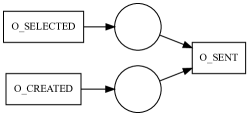
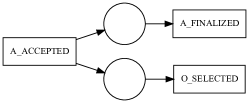
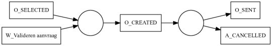
Figure 3: The three highest-ranked representative LPMs for BPIC2012-res10939.

6.2 Local Process Model Diversity Analysis

In Section 5, we introduced how to reduce a set of LPMs LPM to a subset of representative models $\sqcap_{\textit{LPM}}^{\textit{repr}}$ given a cluster set $\sqcap_{\textit{LPM}}$. In this part, we show how significant is the decrease from the original to the representative set for the most compact clusterings, and whether the set of $n$ highest-ranked LPMs in the representative set is more diverse than the set of $n$ highest-ranked LPMs in the original set.

We start by considering the $5$, $10$, $20$, $50$, $100$, and $500$ highest-ranked LPMs obtained on each of the event logs, that is, the sets $\textit{LPM}^{(5)}_{L}$, $\textit{LPM}^{(10)}_{L}$, $\textit{LPM}^{(20)}_{L}$, $\textit{LPM}^{(50)}_{L}$, $\textit{LPM}^{(100)}_{L}$, and $\textit{LPM}^{(500)}_{L}$, where $L$ represents the event logs in Table 1. In Figure 4, we illustrate the decrease in the number of LPMs discovered on the BPIC2012-res10939 and Sepsis event logs for the different similarity measures. The number $n$, denoting the $n$ highest-ranked models in the original set $\textit{LPM}^{(n)}_{L}$, is shown on the x-axis and the number of representative models in $\sqcap^{\textit{repr}_{\textit{dist}}}_{\textit{LPM}^{(n)}_{L}}$, is on the y-axis. It is clear that according to all similarity measures, the most compact clusterings of the LPMs for the Sepsis event log tend to have more clusters. Meaning, the original set already contains more diverse LPMs, and correspondingly the decrease in the number of models is lower. On the contrary, when considering the BPIC2012-res10939 event log, it is noticeable that there is a mismatch between what different similarity measures consider compact grouping. The node measure prefers a few clusters, while the full measure favors much more clusters. Nevertheless, in both cases, the most conservative reduction still reduces the number of models by at least half. Additionally, it is worth mentioning that although these computations are done for the most compact clusterings in our experiments, in general, the number of clusters is something that can be controlled.

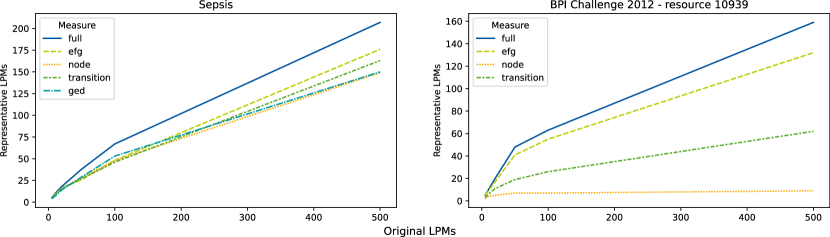
Figure 4: The number of models in the original set (x-axis) versus the number of representative models after clustering (y-axis).

In the second part, we compare the mean distance between all pairs of the $n$ highest-ranked models in the original sets $\textit{LPM}^{(n)}_{L}$, versus the mean distance between all pairs of the $n$ highest-ranked models in the representative sets ${(\sqcap^{\textit{repr}_{\textit{dist}}}_{\textit{LPM}_{L}})}^{(n)}$ for $n=\{5,10,50,100\}$. Figure 5 shows the differences between $\textit{LPM}^{(10)}_{L}$ and ${(\sqcap^{\textit{repr}_{\textit{dist}}}_{\textit{LPM}_{L}})}^{(10)}$ for each of the event logs and the efg measure. It is clear that in all cases the mean distance of the representative set is higher than the mean distance on the original set, meaning the set is more diverse. The highest increase can be noticed for the BPIC2017 event log and the smallest for the BPIC2012-res10939 event log. The distance increase happens for almost all $n$, measure and event log combinations, while for a few no significant change could be noticed.

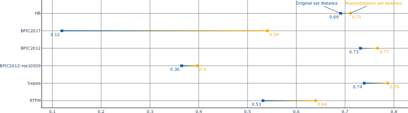
Figure 5: The mean distance between all pairs of LPMs in the original set $\textit{LPM}^{(10)}_{L}$ versus the cluster representative set ${(\sqcap^{\textit{repr}_{\textit{dist}}}_{\textit{LPM}_{L}})}^{(10)}$ and the efg measure.

7 Conclusion

In this paper, we used process model similarity measures to group similar LPMs together. We proposed a three-step approach consisting of LPM discovery, clustering, and choosing LPM cluster representatives. In the evaluation, we showed how grouping similar LPMs together improves process understandability on a real-life case study and we showcased LPM repetition decrease and diversity improvement on six real event logs.

There are numerous possibilites for future work. Currently, we experimented only on one LPM discovery approach, hence, we can expand this work by considering LPMs discovered with different algorithms. To further advance the method, one can also organize the LPMs in each cluster set in hierarchies for more structured navigation between the models. Additionally, the framework could be extended with new similarity measures and different clustering algorithms. Finally, a natural extension would be to test whether LPMs can be used to compare process model similarity measures in an unsupervised manner.

References

- [1] van der Aalst, W.M.P.: Process Mining - Data Science in Action, Second Edition
- [2] Abu-Aisheh, Z., Raveaux, R., Ramel, J., Martineau, P.: An exact graph edit distance algorithm for solving pattern recognition problems. In: ICPRAM 2015. vol. 1, pp. 271–278
- [3] Acheli, M., Grigori, D., Weidlich, M.: Efficient discovery of compact maximal behavioral patterns from event logs. In: CAiSE 2019
- [4] Becker, M., Laue, R.: A comparative survey of business process similarity measures. Comput. Ind. 63(2), 148–167
- [5] Brunings, M., Fahland, D., Verbeek, E.: Discover context-rich local process models (extended abstract). In: ICPM-D 2022
- [6] Deeva, G., Weerdt, J.D.: Understanding automated feedback in learning processes by mining local patterns. In: BPM 2018 International Workshops. vol. 342, pp. 56–68
- [7] Delcoucq, L., Lecron, F., Fortemps, P., van der Aalst, W.M.P.: Resource-centric process mining: clustering using local process models. In: SAC ’20: The 35th ACM/SIGAPP Symposium on Applied Computing, online event, [Brno, Czech Republic], March 30 - April 3, 2020. pp. 45–52
- [8] Dijkman, R.M., van Dongen, B.F., Dumas, M., García-Bañuelos, L., Kunze, M., Leopold, H., Mendling, J., Uba, R., Weidlich, M., Weske, M., Yan, Z.: A short survey on process model similarity. In: Seminal Contributions to Information Systems Engineering, 25 Years of CAiSE, pp. 421–427
- [9] Dumas, M., García-Bañuelos, L., Dijkman, R.M.: Similarity search of business process models. IEEE Data Eng. Bull. 32(3), 23–28
- [10] Kirchner, K., Markovic, P.: Unveiling hidden patterns in flexible medical treatment processes - A process mining case study. In: ICDSST 2018. vol. 313, pp. 169–180
- [11] Kuhn, H.W.: The hungarian method for the assignment problem. In: 50 Years of Integer Programming 1958-2008 - From the Early Years to the State-of-the-Art, pp. 29–47
- [12] Leemans, S.J.J., Tax, N., ter Hofstede, A.H.M.: Indulpet miner: Combining discovery algorithms. In: OTM 2018. vol. 11229, pp. 97–115
- [13] Mannhardt, F., de Leoni, M., Reijers, H.A., van der Aalst, W.M.P., Toussaint, P.J.: Guided process discovery - A pattern-based approach. Inf. Syst. 76, 1–18
- [14] Mannhardt, F., Tax, N.: Unsupervised event abstraction using pattern abstraction and local process models. In: RADAR+EMISA 2017. vol. 1859, pp. 55–63
- [15] Pedregosa, F., et al.: Scikit-learn: Machine learning in Python. Journal of Machine Learning Research 12, 2825–2830
- [16] Peeva, V., Mannel, L.L., van der Aalst, W.M.P.: From place nets to local process models. In: PETRI NETS 2022
- [17] Pijnenborg, P., Verhoeven, R., Firat, M., Laarhoven, H.v., Genga, L.: Towards evidence-based analysis of palliative treatments for stomach and esophageal cancer patients: a process mining approach. In: ICPM 2021. pp. 136–143
- [18] Schoknecht, A., Thaler, T., Fettke, P., Oberweis, A., Laue, R.: Similarity of business process models - A state-of-the-art analysis. ACM Comput. Surv. 50(4), 52:1–52:33
- [19] Tax, N., Sidorova, N., Haakma, R., van der Aalst, W.M.P.: Mining local process models. J. Innov. Digit. Ecosyst. 3(2), 183–196
- [20] Thaler, T., Schoknecht, A., Fettke, P., Oberweis, A., Laue, R.: A comparative analysis of business process model similarity measures. In: BPM 2016 International Workshops. vol. 281, pp. 310–322