A cosmic glitch in gravity
Abstract
We investigate a model that modifies general relativity on cosmological scales, specifically by having a ‘glitch’ in the gravitational constant between the cosmological (super-horizon) and Newtonian (sub-horizon) regimes, as motivated e.g. in the Hořava–Lifshitz proposal or in the Einstein-aether framework. This gives a single-parameter extension to the standard CDM model, which is equivalent to adding a dark energy component, but where the energy density of this component can have either sign. Fitting to data from the Planck satellite, we find that negative contributions are, in fact, preferred. Additionally, we find that roughly one percent weaker superhorizon gravity can somewhat ease the Hubble and clustering tensions in a range of cosmological observations, although at the expense of spoiling fits to the baryonic acoustic oscillation scale in galaxy surveys. Therefore, the extra parametric freedom offered by our model deserves further exploration, and we discuss how future observations may elucidate this potential cosmic glitch in gravity, through a four-fold reduction in statistical uncertainties.
1 Introduction
Albert Einstein’s proposal of the general theory of relativity (GR) that replaced the Newtonian gravitational force with a dynamical living, breathing spacetime geometry has become the cornerstone of modern physics over the past century, having passed all the empirical tests thrown at it — too many to count here — across diverse scales and regimes [1]. Furthermore, a range of mathematical theorems prove the uniqueness of general relativity, subject to conditions, namely covariance (or absence of a preferred frame of reference) and minimal number of degrees of freedom (or only two polarizations for gravitational waves) [2, 3, 4, 5, 6]. Nevertheless, several motivations, most notably the inconsistency of the postulates of quantum theory with those of general relativity, have pushed theorists to explore beyond this minimal set of assumptions. Furthermore, the existence of a preferred cosmological reference frame (where the cosmic microwave background has no dipole), which in the standard picture carries no physical meaning, suggests scrutinising alternatives in which there is a genuinely special cosmological frame. A consequence of such an idea would be that minimal deviations from general relativity would be expected only on cosmological scales [7, 8], or else would require new degrees of freedom (as in modifications that might occur in the strong gravity regime near black holes).
In lieu of introducing a new length scale, some such theories predict a ‘glitch’ between the gravitational constant that governs cosmology on super-horizon scales (through the Friedmann equation) and Newton’s constant of gravitation, that governs the inverse square law on sub-horizon scales. For example, in the Hořava–Lifshitz proposal for a Lorentz-violating theory of gravity [9], the low energy non-projectible theory predicts [10], where is the coefficient of the mean extrinsic curvature squared term in the theory (with in GR). Alternatively, within the Einstein-Aether framework, the parameter is replaced by which quantifies the coupling of geometry with the divergence of the aether flow [11]. Indeed, it has been shown that the low energy non-projectible Hořava–Lifshitz proposal and the Einstein-aether theory with only non-vanishing are physically identical to the quadratic cuscuton theory [7], an incompressible scalar field theory with a quadratic potential [10]. Consequently, it can be formally proven that none of these theories is distinguishable from general relativity in asymptotically flat spacetimes [12], and thus can only be tested on scales comparable to (or larger than) the cosmological horizon [13]. Using the Friedmann equation
| (1.1) |
it is possible to reinterpret this cosmic glitch in gravity as a dark energy component with a constant density relative to critical density:
| (1.2) |
Over the past couple of decades, experimental results have established cold dark matter with a cosmological constant as the standard model of cosmology (referred to as CDM). Although the CDM model has been extremely successful in explaining a wide range of cosmological observables with only a small number of free parameters, there are some observations that might point to deficiencies in the model. One recent example is an apparent discrepancy between the measurement of 4He abundances in ten extremely metal poor galaxies by the EMPRESS collaboration [14]. Here, standard Big Bang predictions can be reconciled if (1) during nucleosynthesis [15]. But is this the only consequence? The primary goal of this paper is to examine the case for a non-vanishing cosmic glitch for other cosmological observables.
Despite the tremendous success of CDM, the increasing precision of cosmological measurements has revealed several discrepancies between different cosmological probes [16], with the most prominent being the different estimates of the Hubble parameter . This Hubble tension refers to the difference between the estimates of based on the distance ladder and the determinations inferred from cosmic microwave background (CMB) anisotropies interpreted through a cosmological model. This discrepancy has now reached perhaps significance between the value derived from Planck satellite data [17, 18, 19] under the CDM model and the value from the SH0ES project using Cepheid-calibrated Type Ia supernovae [20, 21, 22].
In light of this tension, growing efforts have been made to explore the possibility of new physics beyond the CDM model. Many models of non-minimal dark energy beyond a cosmological constant have been proposed and developed, with the goal of solving the Hubble tension in addition to other phenomenological and theoretical motivations. A popular subclass of these models is the early dark energy (EDE) idea, where the modified dark energy component has the greatest impact during the early phase of the Universe, before cosmological recombination [23]. Several EDE models have been developed and tested over the years [24, 25, 26, 27, 28], with various degrees of success on addressing the Hubble tension, depending on the particular model and the data used [27, 28, 29, 30, 31].
An additional tension seen in cosmological observables is the inferred value of the parameter between galaxy weak lensing and CMB measurements [e.g. 32]. More generally, there is a tension between galaxy clustering measurements and CMB measurements in a 2-dimensional plane [e.g. 33]. EDE models that try to address the tension typically do not improve this clustering tension. We will investigate these two tensions for our CGG model.
The CGG parameterisation that we adopt here is similar to the particular EDE model proposed by Doran and Robbers [24], which has been constrained in Ref. [26] with Planck 2015 data and further extended with more parameters in Refs. [25, 34]. In these previous works, the density of the EDE component is always assumed to be positive, which leads to a particularly tight (though one-sided) constraint on [26]. In contrast, we shall relax the positive requirement on and allow it to take negative values in order to fully explore the parameter space and exploit the degeneracy between and . We constrain the model using the Planck 2018 data [18] and discuss the prospect of alleviating the and tensions.
The remainder of the paper is organised as follows. In section 2, we present our phenomenological implementation of the CGG model and its effects on the CMB power spectra. We then provide the constraints on using the cosmological data in section 3, including a discussion of the Hubble constant (section 3.1) and clustering (section 3.2) tensions, as well as consideration of Bayesian model comparisons between CDM and CGG models (section 3.3). In section 4 we discuss the impact of replacing the Planck18 likelihood, which comes from the Planck Public Release 3 (PR3), with the recent LoLLiPoP and HiLLiPoP likelihoods [19] from the Planck Public Release 4 (PR4). We provide forecasts on constraints with future cosmological measurements in section 5, discuss the possibility that the strength of the glitch might vary over time in section 6, and conclude in section 7. Except where explicitly stated otherwise, all parameter uncertainties are given as , which corresponds to the 68 confidence interval for a Gaussian distribution.
2 The phenomenological model
In our model, following eq. 1.2, the energy density of the effective dark energy component is given by
| (2.1) |
In addition to the constant dark energy density in the CDM model, we introduce an extra component that is proportional to the critical density of the Universe, with being the proportionality constant.111Here is a parameter that does not vary with time. Our model, therefore, modifies the amount of gravity for the background. Since also includes , we can isolate from eq. 2.1 to obtain
| (2.2) |
where , which represents the densities of matter, radiation and massless and massive neutrinos, respectively. We consider a flat cosmology with throughout this paper, and we set the effective number of relativistic species222Note that for compatibility with older computation runs we are using the value , here, even though the default value in Cobaya has been changed to . and we assume a single massive neutrino with a mass of . Note that our model described in eq. 2.1 is entirely consistent with the inclusion of massless and massive neutrinos.
Since dominates over in the late Universe, in eq. 2.2 the dynamics of this modified DE model is similar to CDM during late times, but with a slightly different dark energy density due to the denominator , while the dynamics of is substantially altered in the early Universe by tracking the behaviour of radiation and matter densities, respectively, during the radiation-dominated and matter-dominated eras.
Using eq. 2.2, the equation of state parameter for our model can then be written as
| (2.3) |
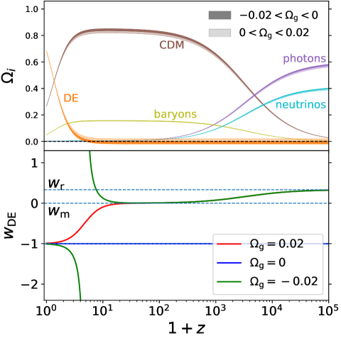
where , , and the equation of state for massive neutrinos can be computed numerically in the code CAMB [35]. As illustrated in the lower panel of figure 1, the CGG model tracks the component that dominates the density of the Universe, with transiting from to and then close to as the Universe evolves. The transition of is smooth for positive , and the dynamics of our is similar to the EDE parameterisation in Ref. [24]. However, for negative values, in eq. 2.2 is negative at early times and becomes positive at late times (the orange region in the upper panel of figure 1). The transition of from negative to positive values causes the diverging behaviour of (the green line) in the lower panel of figure 1. Negative values of typically lead to ghost instabilities in dynamical dark energy models [36, 37], but here we can consider the model with negative as an approximate phenomenological description of modified gravity models, as described above. Some other models with effective dark energy density switching from negative to positive have also been discussed in the literature [28, 38, 39].
There are motivations for adding a component that tracks the total density of the Universe, an example being the cuscuton model [40, 7, 10], which naturally arises when trying to minimally modify GR by introducing a scalar field that does not propagate any new degrees of freedom. When the scalar field has a quadratic potential , the potential minimum contributes towards the cosmological constant, while the quadratic term maintains a constant fraction of the total energy density of the Universe [7], which motivates the specific tracking behaviour introduced in eq. 2.1 for . For negative values we get at late times, which suggests that the model crosses the so-called “phantom divide”. While a single (minimally-coupled) scalar field is gravitationally unstable at such a crossing, a double-field description has been applied to an extension of the CAMB framework to solve the perturbation equations [41], and we shall adopt this approach for our analysis.333The similarity of predictions from this framework, and the incompressible cuscuton limit was verified in Ref. [13]. At the background level, a negative is equivalent to a smaller Newtonian gravitational constant in the Friedman equation, .
In order to obtain the CMB anisotropy and matter power spectra with non-zero , we modify the DarkEnergyFluid module of CAMB [35] where we numerically implemented eqs. 2.2 and 2.3. At the perturbation level, we consider the CGG component as a perfect fluid. Similarly to the approach taken in Refs. [42], we make use of the parameterised post-Friedmann framework proposed in Ref. [41, 43], which is implemented as the DarkEnergyPPF module in CAMB, to allow to be negative. The parameterised post-Friedmann framework approximates the perturbation of the dark energy fluid assuming that it is smooth compared to dark matter, has vanishing anisotropic stress, and a rest frame speed of sound approximately equal to the speed of light [43], allowing the study of a generic dark energy sector with arbitrary .
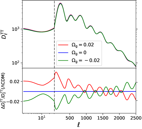
We plot the CMB temperature power spectrum with different values (while fixing all the other parameters to the Planck best-fit values for CDM) in figure 2. We see that a positive increases the integrated Sachs-Wolfe (ISW) effect at low multipoles , along with a slight suppression of the small-scale power in , which is consistent with the predicted behaviour of the quadratic cuscuton [7]. A negative reverses these trends.
3 Constraints on the model
Without a theoretically preferred , we can constrain its value using cosmological observations of the CMB and large-scale structure (LSS). We shall first constrain our CGG model from eq. 2.1, which is a one parameter-extension to the 6-parameter CDM model consisting of ,444We elect to use instead of as the third parameter, which is more appropriate when combining with other data sets such as SH0ES. using the 2018 Planck +low+lensing likelihoods (hereafter referred to as Planck18) [17, 18]. This can be compared to the 6-parameter CDM fits. Our results were computed using the nested sampler PolyChord [44, 45] interfaced with Cobaya [46] and and a modified version of CAMB [35] that implements our CGG model. The priors used in the the nested sampler are given in table 1. To check the robustness of our constraints, we also perform a Markov chain Monte Carlo (MCMC) analysis through Cobaya for each model with broader priors compared to bounds given in table 1, and the MCMC constraints agree with those obtained with nested sampling. We obtain parameter confidence intervals from the nested sampling results using GetDist [47]. The constraints of the main six parameters with and without are reported in table 2 and plotted in figure 3, and the constraints for the three derived parameters of interest together with the constraints for and are shown in figure 4.
| [0.019,0.025] | [0.095,0.145] | [50,90] | [0.01,0.8] | [2.5,3.7] | [0.9,1.1] | [0.06,0.06] |
| Parameter | Planck18 [CDM] | Planck18 [CGG] | Planck18 [CGG] |
| best fit | |||
| 0.0225 | |||
| 0.1162 | |||
| 68.84 | |||
| 0.0507 | |||
| 3.034 | |||
| 0.971 | |||
| 0.0098 | |||
| 0.294 | |||
| 0.834 | |||
| 0.826 |
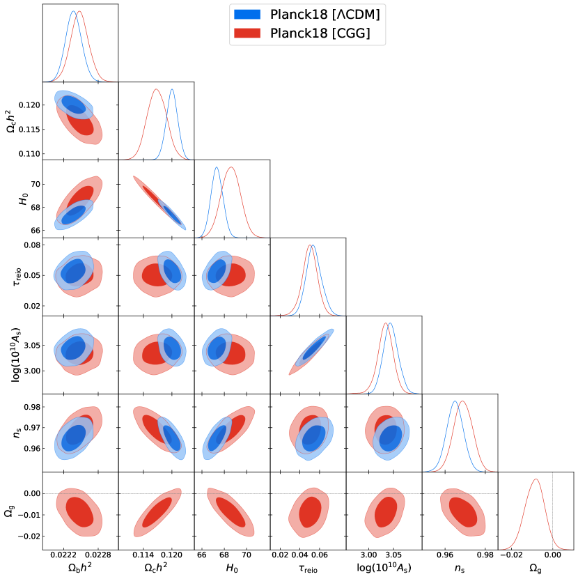
As seen in both table 2 and figure 3, the 2018 Planck data prefer in the negative region, with a value of order 1 %. The CDM model, which corresponds to the CGG model with fixed , is almost away from the mean value in CGG. The parameter is most degenerate with the matter density and the Hubble parameter , in such a way that a negative allows a lower matter density at the present time and a higher Hubble expansion rate, while the constraints for the other four main cosmological parameters remain essentially unchanged. The degeneracy between and can somewhat alleviate the Hubble tension, which we will discuss in section 3.1.
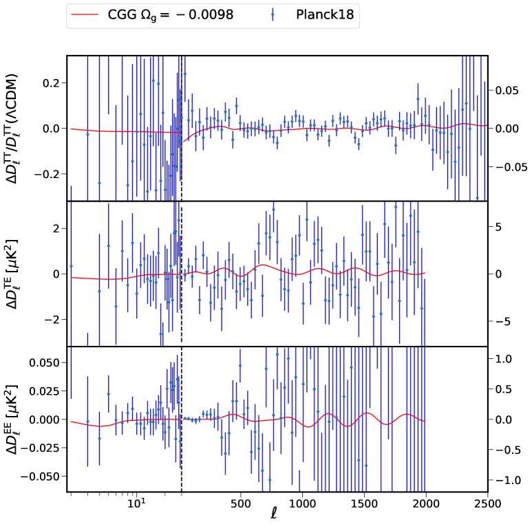
To see why Planck18 data prefer a negative value, we examine the best-fit parameters in both CDM and CGG, and compare the predicted power spectra of these best-fit results to the measured Planck power spectra. As seen in table 3 and figure 5, the CGG model with negative lowers the low- part of the and power spectra, which provides a slightly better fit to the “low- deficit” [48, 18] observed in the measured CMB power spectra. For the high- part of the and power spectra, the CGG model provides a slightly better fit to the apparent oscillations in the residuals between the measured Planck18 power spectra and the best-fit CDM model (the first two panels of figure 5), which account for most of the overall improvement (the third row of table 3).
| Data Set | CDM | CGG | |
|---|---|---|---|
| low- TT | 23.3 | 22.1 | |
| low- EE | 396.0 | 395.6 | |
| high- TTTEEE | 2344.9 | 2342.1 | |
| lensing | 8.9 | 9.7 | 0.8 |
| total | 2773.1 | 2769.5 |
If we restrict to the positive region, we find and for the and confidence intervals, which is consistent with the constraints on under similar EDE parametrizations [26, 34]. Thus, we discover for the first time that the extremely tight constraint on for the EDE models in the literature is because Planck CMB data—in fact—favour negative values.
3.1 Hubble tension
We now discuss the constraint on in our CGG model with Planck18 data in light of the Hubble tension. In recent years, the value of the Hubble constant inferred from probes of the early Universe from the CMB [18] has been in persistent disagreement with distance-ladder-derived estimates from the late Universe, a discrepancy that has now reached roughly the level [20, 21, 22]. For example, in [21], the Hubble constant is estimated to be (hereafter referred to as SH0ES) in contrast to the Planck18 value of .
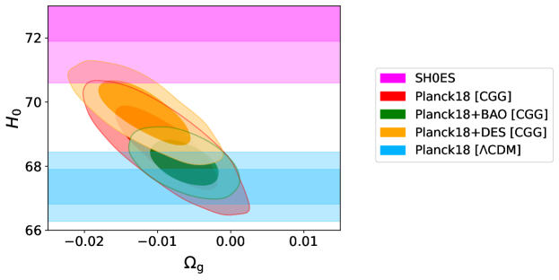
With our CGG model under Planck18, is determined to be , which is higher than the CDM value, thus somewhat alleviating the Hubble tension. The posterior average of is . The joint constraints for and are plotted in footnote 5, which shows the strong degeneracy between the two parameters. Combining the Planck18 data with baryonic acoustic oscillation (BAO) measurements [49, 50, 51], we obtain and for our CGG model, which is more consistent with the CDM results compared to the CGG fits using the Planck18 data only. Combining the Planck18 data with galaxy clustering and weak gravitational lensing measurements from the Dark Energy Survey (DES) [52], we obtain and , which is slightly higher than the measurements from our CGG model using Planck18 data only. These constraints are summarised in footnote 5. Adding the Pantheon Supernovae (SNe) likelihood [53] to the Planck18 data only very slightly shrinks the constraints on and , with and , leaving the corresponding contours from figure 3 essentially indistinguishable.
Our CGG model with only one additional parameter eases the Hubble tension (from 4.1 to 3.0) when we only consider the 2018 Planck measurements of the CMB. Allowing to be negative helps to reconcile the Hubble tension, since a lower corresponds to a higher value. Adding DES Y1 data further increases the preferred , to within of the local SH0ES measurement. However, adding BAO data to the Planck18 measurements tightens the constraint of , while lowering the mean value to away from the value in Ref. [22]. The summary is that although the CGG model somewhat alleviates the tension, the situation is complicated and depends on the choice of data set. Moreover, we need to consider the statistical effect of adding an additional parametric degree of freedom to the fits, which we will discuss in section 3.3.
3.2 Clustering tension
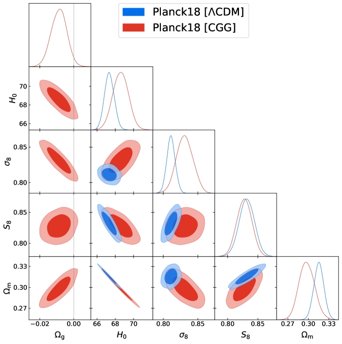
As illustrated in figure 4, is also correlated in the fits with and . However, the negative value increases the fitted value compared to the CDM results, which does not alleviate the tension. To obtain a lower value, we would need a positive , which is disfavoured by the Planck18 data. Adding massive neutrinos as a free parameter to our CGG model would be one way to help with the tension, since increasing the mass of neutrinos will lead to a lower constraint based on the Planck data. Turning to the tension, our model does not shift the constraint, since and receive opposite shifts that essentially cancel in the combination. Therefore, the CGG model neither alleviates nor worsens the tension, which is similar to other EDE models [54]. Note that is anti-correlated with , so a lower value corresponds to a higher value, as seen in figure 4.
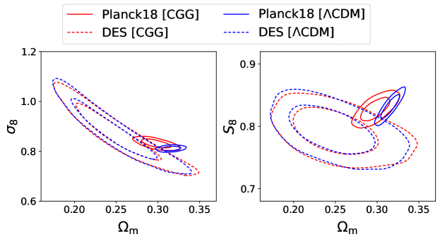
Considering the 2-dimensional (2D) representation of the clustering tension, we plot the constraints on and using Planck18 data and DES data in figure 7. DES data alone have little constraining power on , and the constraints of and for DES under the CGG model are similar to those under CDM. However, the CGG model noticeably lowers the best-fit for under the Planck18 data by allowing negative values (figure 4). As a result, the – confidence region of DES and that of Planck18 have a larger area of overlap under the CGG model compared to the CDM case, as seen in the right panel of figure 7. Therefore, the clustering tension is in fact slightly alleviated by the CGG model when we view the tension in the 2D plane formed by and instead of only considering the single parameter . The situation for the – 2D plane is similar (left panel in figure 7).
3.3 Model comparison
To properly account for the increased volume of the parameter space under the CGG model over CDM, we perform a Bayesian model comparison by calculating the difference of Bayesian evidence , which naturally incorporates the so-called Occam’s razor that penalises models for unnecessary complexity. For Bayesian model comparison, we follow the procedure outlined in Ref. [55] using the nested sampler PolyChord [44, 45] to explore the parameter space (the priors of the cosmological parameters are specified in table 1), and using anesthetic [56] for the computation of Bayesian evidence, Kullback–Leibler divergence, and further statistics.
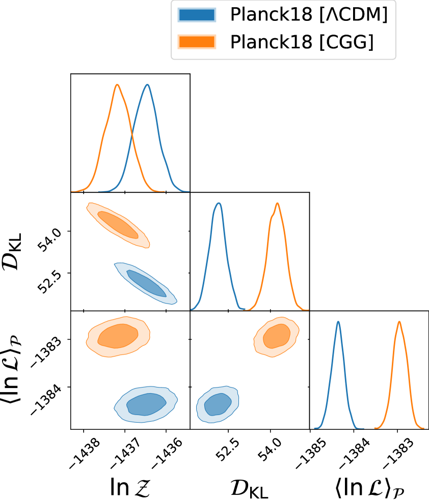
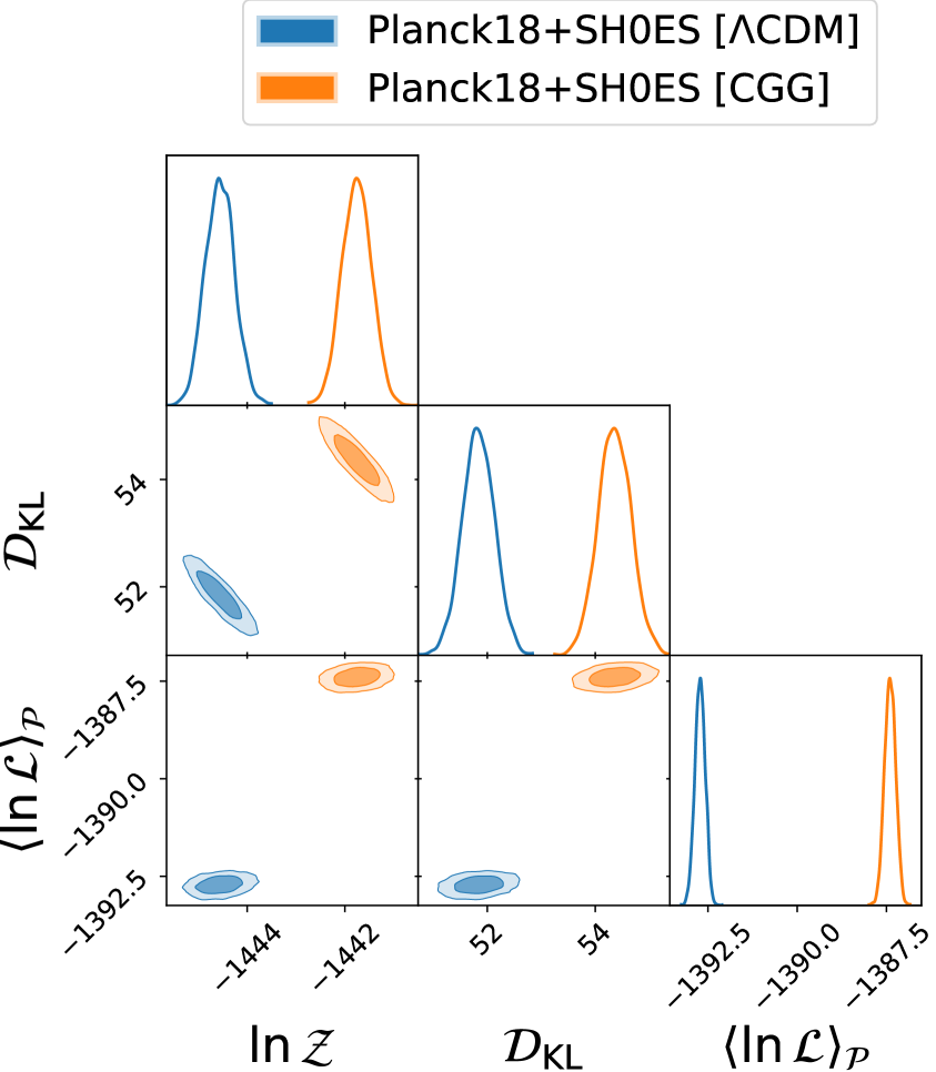
As seen in figure 8(a), although the CGG model provides a better fit to the Planck18 data, the improvement in the fit is not sufficient to compensate for the increase in complexity measured by the Kullback–Leibler divergence . The two models are on-par with each other under the Planck18 likelihood in terms of Bayesian evidence . However, if we perform the Bayesian model comparison under both the Planck18 and SH0ES likelihoods (figure 8(b)), we see that the log-evidence under the CGG model is higher than that under CDM, with a significantly better fit overcoming the penalty from the higher complexity of having an additional parameter. In this case, we have , suggesting that the CGG model is clearly favoured (although not conclusively), over the CDM model under the Planck18+SH0ES likelihood. This reflects how the extensions helps alleviate the Hubble tension between Planck18 and SH0ES.
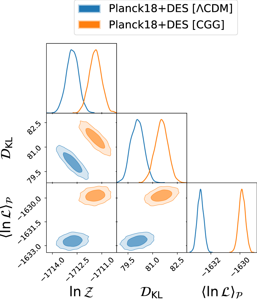
As for the model performance under the DES data only, the statistics considered here have consistent values, up to sampling uncertainties, for the CGG and the CDM models. Under both the Planck18 and DES likelihoods, we see in figure 8(c) that the CGG model is slightly preferred over CDM by (although the sampling uncertainty for the estimate here is about 0.5), which indicates the slight alleviation of the clustering tension based on model comparison. Using suspiciousness [33, 57], which can quantify the global tension between two dataset and over the entire parameter space, the tension between Planck18 and DES reduces from 2.2 (CDM) to 2 (CGG), which reflects the slight alleviation of the clustering tension by adding .
4 Impacts of Planck PR4 data
Since this work was completed, a new analysis of the Planck Public Release 4 (PR4) data set [58] has been published, using the LoLLiPoP (low-) and HiLLiPoP (high-) likelihoods [19]. This new likelihood analysis of Planck data yields tighter constraints, as well as slightly shifting results for some previous claims of parameter anomalies (e.g. the lensing consistency parameter ) [19]. For this reason, it is useful to check how much the constraints on the CGG model change if we use the PR4 data rather than the Planck18 data (also known as PR3).
We have derived cosmological constraints on the CGG model using the HiLLiPoP (high- TTTEEE), LoLLiPoP (low- EE), and CMB lensing likelihoods [59] based on Planck PR4. The only part of the PR4 analysis still relying on the Planck18 (PR3) data is the low- temperature likelihood. Under the PR4 analysis, all parameter constraints of the CGG model are slightly tighter compared to the PR3 analysis. In particular, we find that and . The CDM model, which corresponds to the CGG model with fixed , is now away from the mean value in CGG under the PR4 analysis, compared to the preference for negative values under the PR3 analysis. It is interesting to notice that the shift of (from to ) is significantly less than the shifts of and from the PR3 to PR4 analysis observed in Ref. [19]. The PR4 likelihood still prefers negative values, albeit to a slightly less extent compared to the PR3 results.
For the clustering parameters, Planck PR4 is known to relieve the clustering tension compared to PR3 [19] already for the CDM model. This is still the case for the CGG model, alhough to a smaller degree, since the tension is already considerably decreased by switching from CDM to CGG. For the clustering parameters under the CGG model, we find and .
5 Forecasts for future CMB and BAO measurements
| Parameter | Current CMB | Ideal CMB | Ideal CMB+Euclid BAO |
|---|---|---|---|
As discussed in sections 3 and 4, the current cosmological data favour a negative value. To distinguish whether is truly negative or consistent with 0, we will need better data. So we now consider the constraining power of future cosmological measurements on . To give a simplistic assessment of this idea, we combine the Fisher forecasts from an ideal cosmic variance limited (CVL) CMB experiment and the measurements of the BAO scale in a Euclid-like survey [61]. The details of the Fisher forecast method are described in Appendix A of Ref. [60]. For the CVL CMB forecast, we make use of the , and power spectra ( up to for and for ) along with the lensing reconstruction spectra for up to 1000. As shown in table 4, the CVL CMB alone can achieve a uncertainty of around , while adding Euclid-like BAO data can improve the constraint to below , which is approximately a four fold reduction of uncertainty compared to the current constraints. With such small uncertainties, we should be able to distinguish whether is truly negative or consistent with CDM in the upcoming stage IV CMB [62] and LSS surveys [61, 63]. Since our model mostly modifies the equation of state for dark energy at high redshift, we expect that future LSS surveys [64, 65] focusing on will be particularly promising for constraining the cosmic glitch parameter .
6 The possibility of non-constant
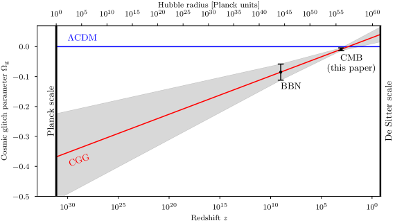
In addition to the and tensions, there may be differences in the early Universe. We noted in the introduction that an independent piece of evidence for a negative comes from measurements of helium abundance in extremely low metallicity galaxies, and its incompatibility with nucleosynthesis in the standard model [15]. However, the value of required to reconcile the measurements is significantly smaller than the constraints found here coming from fits to the Planck 2018 data.666Incidentally, we checked that having a different at the Big Bang nucleosynthesis epoch, which would change the primordial helium abundance , has a negligible effect on the parameter constraints presented in table 2. Given that these values affect comic dynamics in vastly different eras, one may speculate about a logarithmic running of the cosmic glitch with scale, similar to other fundamental dimensionless constants in renormalizable theories. Figure 9 shows the values of these measurements, along with the possible linear extrapolations expected from a renormalisation group flow. This suggests a possible scenario where the glitch vanishes on the scale of the observed cosmological constant (or de Sitter radius) today, where we recover near-exact de Sitter symmetry. In contrast, at the Big Bang (or Planck scale), the glitch parameter is , pointing to a significant violation of general covariance in a quantum theory of gravity. This may further hint at a genuine quantum gravity solution to the cosmological horizon problem, which is traditionally solved using an inflationary paradigm (e.g. [66]).
7 Conclusions
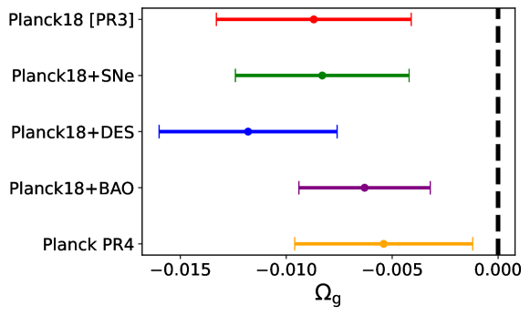
In this paper, we have examined the theoretical and observational cases for a cosmic glitch in gravity, i.e. a model in which gravity is different for super-horizon and sub-horizon scales, as a minimal modification of Einstein’s general relativity without introducing any new scale or degree of freedom. The best-fit CGG model prefers a higher and lower than CDM, but the value of has hardly changed. On the other hand, we find that the Planck 2018 data favour a negative cosmic glitch parameter , a parameter region that has not been explored before. The significance of the evidence for this glitch ranges from 1.9 to 2.8, depending on the additional large-scale structure data used in the analysis, while it decreases to 1.3 when using only CMB data and replacing the Planck 2018 (PR3) likelihoods with the newer likelihoods based on Planck PR4. We provide a summary of the constraints on in figure 10.
By analysing the parameter constraints and performing a Bayesian model comparison, we see that our CGG model somewhat alleviates both the Hubble parameter and the clustering tensions when using the Planck 2018 data, while the constraint using the Planck 2018 and DES Y1 data is compatible with the local SH0ES measurement. In contrast, including the observed BAO scale spoils this agreement on . However, it is possible that current BAO scale measurements may be biased or their uncertainties might be underestimated for this class of non-CDM cosmology [67, 68], something that requires further calibration in mock observations. Nevertheless, this effectively negative early dark energy component, realised through the CGG, deserves more study. Future CMB and large-scale structure data (such as DESI or Euclid) will inevitably tighten these bounds and shed light on whether a cosmic glitch in gravity is responsible for some of our current cosmic tensions.
Acknowledgments
This research was supported by the Natural Sciences and Engineering Research Council of Canada. NA is further supported by the Perimeter Institute for Theoretical Physics. Research at Perimeter Institute is supported in part by the Government of Canada through the Department of Innovation, Science and Economic Development Canada and by the Province of Ontario through the Ministry of Colleges and Universities. LTH was supported by a Killam Postdoctoral Fellowship and a CITA National Fellowship. Computing resources were provided by the Digitial Research Alliance of Canada/Calcul Canada (alliancecan.ca). Parts of this paper are based on observations obtained with Planck (www.esa.int/Planck), an ESA science mission with instruments and contributions directly funded by ESA Member States, NASA and Canada. This paper made use of the codes CAMB (camb.readthedocs.io/en/latest/) and Cobaya (cobaya.readthedocs.io/en/latest/).
References
- [1] C. M. Will and N. Yunes, Is Einstein Still Right?: Black Holes, Gravitational Waves, and the Quest to Verify Einstein’s Greatest Creation. Oxford University Press, USA, 2020.
- [2] D. Lovelock, The Four-Dimensionality of Space and the Einstein Tensor, Journal of Mathematical Physics 13 (1972) 874.
- [3] K. Kuchař, Geometrodynamics regained: A Lagrangian approach, Journal of Mathematical Physics 15 (1974) 708.
- [4] s. a. hojman, K. Kuchař and C. Teitelboim, Geometrodynamics regained, Annals of Physics 96 (1976) 88.
- [5] J. Khoury, G. E. Miller and A. J. Tolley, Spatially covariant theories of a transverse, traceless graviton: Formalism, Physical Review D 85 (2012) 084002.
- [6] K. Krasnov and E. Mitsou, Pure lorentz spin connection theories and uniqueness of general relativity, Classical and Quantum Gravity 38 (2021) 205009.
- [7] N. Afshordi, D. J. H. Chung, M. Doran and G. Geshnizjani, Cuscuton cosmology: Dark energy meets modified gravity, Phys. Rev. D 75 (2007) 123509 [astro-ph/0702002].
- [8] S. Mukohyama and K. Noui, Minimally modified gravity: a hamiltonian construction, Journal of Cosmology and Astroparticle Physics 2019 (2019) 049.
- [9] P. Hořava, Quantum gravity at a lifshitz point, Physical Review D 79 (2009) 084008.
- [10] N. Afshordi, Cuscuton and low-energy limit of Hořava-Lifshitz gravity, Phys. Rev. D 80 (2009) 081502 [0907.5201].
- [11] T. Jacobson, Extended hořava gravity and einstein-aether theory, Physical Review D 81 (2010) 101502.
- [12] R. Loll and L. Pires, Role of the extra coupling in the kinetic term in Hořava-Lifshitz gravity, Phys. Rev. D 90 (2014) 124050 [1407.1259].
- [13] G. Robbers, N. Afshordi and M. Doran, Does Planck mass run on the cosmological horizon scale?, Phys. Rev. Lett. 100 (2008) 111101 [0708.3235].
- [14] A. Matsumoto, M. Ouchi, K. Nakajima, M. Kawasaki, K. Murai, K. Motohara et al., Empress. viii. a new determination of primordial he abundance with extremely metal-poor galaxies: A suggestion of the lepton asymmetry and implications for the hubble tension, The Astrophysical Journal 941 (2022) 167.
- [15] K. Kohri and K.-i. Maeda, A possible solution to the helium anomaly of EMPRESS VIII by cuscuton gravity theory, Progress of Theoretical and Experimental Physics 2022 (2022) 091E01 [2206.11257].
- [16] E. Abdalla, G. F. Abellán and A. Aboubrahim et al., Cosmology intertwined: A review of the particle physics, astrophysics, and cosmology associated with the cosmological tensions and anomalies, Journal of High Energy Astrophysics 34 (2022) 49 [2203.06142].
- [17] Planck Collaboration V, Planck 2018 results. V. Power spectra and likelihoods, A&A 641 (2020) A5 [1907.12875].
- [18] Planck Collaboration VI, Planck 2018 results. VI. Cosmological parameters, A&A 641 (2020) A6 [1807.06209].
- [19] M. Tristram, A. J. Banday, M. Douspis, X. Garrido, K. M. Górski, S. Henrot-Versillé et al., Cosmological parameters derived from the final (PR4) Planck data release, arXiv e-prints (2023) arXiv:2309.10034 [2309.10034].
- [20] A. G. Riess, S. Casertano, W. Yuan, L. M. Macri and D. Scolnic, Large Magellanic Cloud Cepheid Standards Provide a 1% Foundation for the Determination of the Hubble Constant and Stronger Evidence for Physics beyond CDM, ApJ 876 (2019) 85 [1903.07603].
- [21] A. G. Riess, S. Casertano, W. Yuancob, J. B. Bowers, L. Macri, J. C. Zinn et al., Cosmic Distances Calibrated to 1% Precision with Gaia EDR3 Parallaxes and Hubble Space Telescope Photometry of 75 Milky Way Cepheids Confirm Tension with CDM, ApJ 908 (2021) L6 [2012.08534].
- [22] A. G. Riess, W. Yuan, L. M. Macri, D. Scolnic, D. Brout, S. Casertano et al., A Comprehensive Measurement of the Local Value of the Hubble Constant with 1 km s-1 Mpc-1 Uncertainty from the Hubble Space Telescope and the SH0ES Team, ApJ 934 (2022) L7 [2112.04510].
- [23] V. Poulin, T. L. Smith and T. Karwal, The Ups and Downs of Early Dark Energy solutions to the Hubble tension: a review of models, hints and constraints circa 2023, arXiv e-prints (2023) arXiv:2302.09032 [2302.09032].
- [24] M. Doran and G. Robbers, Early dark energy cosmologies, JCAP 2006 (2006) 026 [astro-ph/0601544].
- [25] V. Pettorino, L. Amendola and C. Wetterich, How early is early dark energy?, Phys. Rev. D 87 (2013) 083009 [1301.5279].
- [26] Planck Collaboration, Planck 2015 results. XIV. Dark energy and modified gravity, A&A 594 (2016) A14 [1502.01590].
- [27] V. Poulin, T. L. Smith, T. Karwal and M. Kamionkowski, Early Dark Energy can Resolve the Hubble Tension, Phys. Rev. Lett. 122 (2019) 221301 [1811.04083].
- [28] G. Ye and Y.-S. Piao, Is the Hubble tension a hint of AdS phase around recombination?, Phys. Rev. D 101 (2020) 083507 [2001.02451].
- [29] J. C. Hill, E. Calabrese, S. Aiola, N. Battaglia, B. Bolliet, S. K. Choi et al., Atacama Cosmology Telescope: Constraints on prerecombination early dark energy, Phys. Rev. D 105 (2022) 123536 [2109.04451].
- [30] J. C. Hill, E. McDonough, M. W. Toomey and S. Alexander, Early dark energy does not restore cosmological concordance, Phys. Rev. D 102 (2020) 043507 [2003.07355].
- [31] J.-Q. Jiang and Y.-S. Piao, Testing AdS early dark energy with Planck, SPTpol, and LSS data, Phys. Rev. D 104 (2021) 103524 [2107.07128].
- [32] E. Abdalla, G. F. Abellán, A. Aboubrahim, A. Agnello, Ö. Akarsu, Y. Akrami et al., Cosmology intertwined: A review of the particle physics, astrophysics, and cosmology associated with the cosmological tensions and anomalies, Journal of High Energy Astrophysics 34 (2022) 49 [2203.06142].
- [33] W. Handley and P. Lemos, Quantifying tensions in cosmological parameters: Interpreting the DES evidence ratio, Phys. Rev. D 100 (2019) 043504 [1902.04029].
- [34] A. Gómez-Valent, Z. Zheng, L. Amendola, V. Pettorino and C. Wetterich, Early dark energy in the pre- and postrecombination epochs, Phys. Rev. D 104 (2021) 083536 [2107.11065].
- [35] A. Lewis, A. Challinor and A. Lasenby, Efficient computation of CMB anisotropies in closed FRW models, ApJ 538 (2000) 473 [astro-ph/9911177].
- [36] E. Ebrahimi and A. Sheykhi, Instability of QCD Ghost Dark Energy Model, International Journal of Modern Physics D 20 (2011) 2369 [1106.3504].
- [37] F. Sbisà, Classical and quantum ghosts, European Journal of Physics 36 (2015) 015009 [1406.4550].
- [38] R. Calderón, R. Gannouji, B. L’Huillier and D. Polarski, Negative cosmological constant in the dark sector?, Phys. Rev. D 103 (2021) 023526 [2008.10237].
- [39] Ö. Akarsu, J. D. Barrow, L. A. Escamilla and J. A. Vazquez, Graduated dark energy: Observational hints of a spontaneous sign switch in the cosmological constant, Phys. Rev. D 101 (2020) 063528 [1912.08751].
- [40] N. Afshordi, D. J. H. Chung and G. Geshnizjani, Causal field theory with an infinite speed of sound, Phys. Rev. D 75 (2007) 083513 [hep-th/0609150].
- [41] W. Hu, Parametrized post-Friedmann signatures of acceleration in the CMB, Phys. Rev. D 77 (2008) 103524 [0801.2433].
- [42] A. Krolewski and S. Ferraro, The Integrated Sachs Wolfe effect: unWISE and Planck constraints on dynamical dark energy, JCAP 2022 (2022) 033 [2110.13959].
- [43] W. Fang, W. Hu and A. Lewis, Crossing the phantom divide with parametrized post-Friedmann dark energy, Phys. Rev. D 78 (2008) 087303 [0808.3125].
- [44] W. J. Handley, M. P. Hobson and A. N. Lasenby, POLYCHORD: next-generation nested sampling, MNRAS 453 (2015) 4384 [1506.00171].
- [45] W. J. Handley, M. P. Hobson and A. N. Lasenby, polychord: nested sampling for cosmology., MNRAS 450 (2015) L61 [1502.01856].
- [46] J. Torrado and A. Lewis, Cobaya: Code for Bayesian Analysis of hierarchical physical models, arXiv e-prints (2020) [2005.05290].
- [47] A. Lewis, GetDist: a Python package for analysing Monte Carlo samples, arXiv e-prints (2019) arXiv:1910.13970 [1910.13970].
- [48] Planck Collaboration Int. LI, Planck intermediate results. LI. Features in the cosmic microwave background temperature power spectrum and shifts in cosmological parameters, A&A 607 (2017) A95 [1608.02487].
- [49] F. Beutler, C. Blake, M. Colless, D. H. Jones, L. Staveley-Smith, L. Campbell et al., The 6dF Galaxy Survey: baryon acoustic oscillations and the local Hubble constant, MNRAS 416 (2011) 3017 [1106.3366].
- [50] A. J. Ross, L. Samushia, C. Howlett, W. J. Percival, A. Burden and M. Manera, The clustering of the SDSS DR7 main Galaxy sample - I. A 4 per cent distance measure at z = 0.15, MNRAS 449 (2015) 835 [1409.3242].
- [51] S. Alam, M. Ata, S. Bailey, F. Beutler, D. Bizyaev et al., The clustering of galaxies in the completed SDSS-III Baryon Oscillation Spectroscopic Survey: cosmological analysis of the DR12 galaxy sample, MNRAS 470 (2017) 2617 [1607.03155].
- [52] T. M. C. Abbott, F. B. Abdalla, A. Alarcon, J. Aleksić, S. Allam, S. Allen et al., Dark Energy Survey year 1 results: Cosmological constraints from galaxy clustering and weak lensing, Phys. Rev. D 98 (2018) 043526 [1708.01530].
- [53] D. M. Scolnic, D. O. Jones, A. Rest, Y. C. Pan, R. Chornock, R. J. Foley et al., The Complete Light-curve Sample of Spectroscopically Confirmed SNe Ia from Pan-STARRS1 and Cosmological Constraints from the Combined Pantheon Sample, ApJ 859 (2018) 101 [1710.00845].
- [54] R. Murgia, G. F. Abellán and V. Poulin, Early dark energy resolution to the Hubble tension in light of weak lensing surveys and lensing anomalies, Phys. Rev. D 103 (2021) 063502 [2009.10733].
- [55] L. T. Hergt, W. J. Handley, M. P. Hobson and A. N. Lasenby, Bayesian evidence for the tensor-to-scalar ratio r and neutrino masses mν : Effects of uniform versus logarithmic priors, Phys. Rev. D 103 (2021) 123511 [2102.11511].
- [56] W. Handley, anesthetic: nested sampling visualisation, The Journal of Open Source Software 4 (2019) 1414.
- [57] W. Handley and P. Lemos, Quantifying the global parameter tensions between ACT, SPT, and Planck, Phys. Rev. D 103 (2021) 063529 [2007.08496].
- [58] Planck Collaboration, Y. Akrami, K. J. Andersen, M. Ashdown, C. Baccigalupi, M. Ballardini et al., Planck intermediate results. LVII. Joint Planck LFI and HFI data processing, A&A 643 (2020) A42 [2007.04997].
- [59] J. Carron, M. Mirmelstein and A. Lewis, CMB lensing from Planck PR4 maps, JCAP 2022 (2022) 039 [2206.07773].
- [60] Y. Wen, D. Scott, R. Sullivan and J. P. Zibin, Role of T0 in CMB anisotropy measurements, Phys. Rev. D 104 (2021) 043516 [2011.09616].
- [61] R. Laureijs, J. Amiaux, S. Arduini, J. L. Auguères, J. Brinchmann et al., Euclid Definition Study Report, arXiv e-prints (2011) [1110.3193].
- [62] K. N. Abazajian, P. Adshead, Z. Ahmed, S. W. Allen, D. Alonso et al., CMB-S4 Science Book, First Edition, arXiv e-prints (2016) [1610.02743].
- [63] DESI Collaboration, The DESI Experiment Part I: Science,Targeting, and Survey Design, arXiv e-prints (2016) [1611.00036].
- [64] A. Slosar, Z. Ahmed, D. Alonso, M. A. Amin, E. J. Arena, K. Bandura et al., Packed Ultra-wideband Mapping Array (PUMA): A Radio Telescope for Cosmology and Transients, in Bulletin of the American Astronomical Society, vol. 51, p. 53, Sept., 2019, 1907.12559, DOI.
- [65] D. Schlegel, J. A. Kollmeier and S. Ferraro, The MegaMapper: a z>2 spectroscopic instrument for the study of Inflation and Dark Energy, in Bulletin of the American Astronomical Society, vol. 51, p. 229, Sept., 2019, 1907.11171, DOI.
- [66] N. Afshordi and J. Magueijo, Critical geometry of a thermal big bang, Phys. Rev. D 94 (2016) 101301 [1603.03312].
- [67] S. Anselmi, P.-S. Corasaniti, A. G. Sanchez, G. D. Starkman, R. K. Sheth and I. Zehavi, Cosmic distance inference from purely geometric BAO methods: Linear point standard ruler and correlation function model fitting, Phys. Rev. D 99 (2019) 123515 [1811.12312].
- [68] S. Anselmi, G. D. Starkman and A. Renzi, Linear Point Standard Ruler: cosmological forecasts for future galaxy surveys. Toward consistent BAO analyses far from a fiducial cosmology, arXiv e-prints (2022) arXiv:2205.09098 [2205.09098].