Breaking the Degrees-of-Freedom Limit of Holographic MIMO Communications: A 3-D Array Topology
Abstract
The efficacy of holographic multiple-input multiple-output (MIMO) communications, employing two-dimensional (2-D) planar antenna arrays, is typically compromised by finite degrees-of-freedom (DOF) stemming from limited array size. The DOF constraint becomes significant when the element spacing approaches approximately half a wavelength, thereby restricting the overall performance of MIMO systems. To break this inherent limitation, we propose a novel three-dimensional (3-D) array topology that strategically explores the untapped vertical dimension. We investigate the performance of MIMO systems utilizing 3-D arrays across different multi-path scenarios, encompassing Rayleigh channels with varying angular spreads and the 3rd generation partnership project (3GPP) channels. We subsequently showcase the advantages of these 3-D arrays over their 2-D counterparts with the same aperture sizes. As a proof of concept, a practical dipole-based 3-D array, facilitated by an electromagnetic band-gap (EBG) reflecting surface, is conceived, constructed, and evaluated. The experimental results align closely with full-wave simulations, and channel simulations substantiate that the DOF and capacity constraints of traditional holographic MIMO systems can be surpassed by adopting such a 3-D array configuration.
Keywords Holographic multiple-input-multiple-output (MIMO) communications Degrees of freedom Channel capacity Degree of freedom MIMO antenna array
1 Introduction
The multiple-input-multiple-output (MIMO) technology, pivotal in wireless communications, has demonstrated substantial capacity enhancement across diverse scenarios, marking considerable success over the years [1, 2, 3]. In the pursuit of augmenting MIMO communication performance, several technologies have been developed. Some representative technologies include massive MIMO communications [4, 5, 6, 7], decoupling and decorrelation of MIMO arrays [8, 9, 10, 11], reconfigurable intelligent surface (RIS) aided MIMO communications [12, 13], and holographic MIMO communications [14, 15, 16, 17, 18, 19]. Holographic MIMO communications, an advanced iteration of RIS, present promising avenues for research in the realm of highly adaptable antennas by skillfully harnessing electromagnetic (EM) waves [20]. Notably, a holographic MIMO array can comprise large amount of antennas within a compact aperture, and it has been substantiated to possess numerous advantages [21].
However, the primary challenge associated with holographic MIMO communications is the finite degrees-of-freedom (DOF) constrained by array size [22]. Given that a holographic MIMO array integrates a substantial number of antennas with sub-wavelength inter-element spacing within a confined area, a pronounced correlation emerges among the antennas, resulting in performance degradation [23]. To compensate such an impaired performance, an increase in array size is expected. Unfortunately, the array sizes at the base station or vehicles in practice are strictly confined. Hence, exceeding the DOF limit is imperative in further enhancing the aperture-constrained MIMO performance from an application standpoint.
In the pursuit of surpassing the DOF limit, it is necessary to make clear the fundamental limits of holographic MIMO communications. This analysis has been undertaken from dual perspectives—both information and electromagnetic (EM)—to provide a comprehensive understanding of the inherent limitations [24, 25, 26, 27, 28, 29, 30, 31]. In typical multi-path environment, the performance of a MIMO system depends on both the power gain and the DOF gain [2]. The power gain is known as the beamforming gain, which is constricted by the aperture size of array [32]. One famous argument is the Hannan’s limit [33], providing the closed-form expression of the radiation efficiency limit of antenna elements when more and more elements are placed into a constrained planar aperture. In addition of the power gain, the DOF gain usually attracts more attentions when dealing with MIMO communications.
The DOF of a MIMO system refers to the effective rank (the number of significant eigenvalues) of its correlation matrix [2], or the number of scattering channels [34], or the number of available spatial EM modes [35], which characterizes the spatial-multiplexing performance of the MIMO system. The DOF of a MIMO system has been discussed based on various models, including the general scattering method [34, 24, 36, 37, 38], the Green’s function method [25, 17, 39, 40, 41], the intuitive methods [35, 42], the plane-wave expansion model [20, 14], etc. These models are essentially equivalent but using different expansion bases of EM waves. As a brief summary, the DOF limit of an aperture-constrained MIMO system is considered to be only dependent on the surface area of the transmitting/receiving space [41, 24], or the average scattering cross-section[30, 29].
Therefore, one possible route to violate the DOF limit of holographic MIMO communications is to build a three-dimensional (3-D) array, which explores the additional volume available in the vertical dimension, and thus extra DOF. Some similar concepts can be found in using the scatterer array over a MIMO array for realizing the de-correlation, thus improving the DOF and capacity [11, 10, 43]. As far as our knowledge extends, neither the concept of breaking the DOF limit by using the 3-D array nor the corresponding performance analyses have been discussed before. In this work, a novel 3-D array topology is proposed for breaking the DOF limit of a conventional holographic MIMO communication system. The contributions of this paper can mainly be attributed to the following three aspects:
-
•
The theoretical analyses of the MIMO performances of 3-D arrays based on the 3-D Clarke and Kronecker models; for example, comparing the performances of the 3-D and two-dimensional (2-D) arrays with the same aperture size at different height differences, element spacings and angular spreads.
-
•
A practical 3-D antenna array enabled by an EM band-gap (EBG) reflecting surface is designed, fabricated and measured as a proof of concept.
-
•
Assessments of the MIMO performances of the practical 3-D array are conducted in both Rayleigh channels with varying angular spreads and 3rd generation partnership project (3GPP) channels.
A comprehensive exploration of the properties of the 3-D array topology in various scenarios is presented in detail. The findings reveal that the 3-D array holds significant promise as a candidate for augmenting MIMO performance in the landscape of future wireless communications.
The rest of this paper is organized as follows. In Section II, the methodology of 3-D array, and the tools for evaluating MIMO performance, i.e., the 3-D Clarke and Kronecker models, are introduced. Next, the theoretical analyses are carried out in Section III based on the two models. After that, the design, simulation and experimental validation of a practical 3-D array, together with the discussion of its MIMO performances in Rayleigh and 3GPP channels, are presented in Section IV. Finally, some remarks and conclusions are given in Section V.
2 Methodology
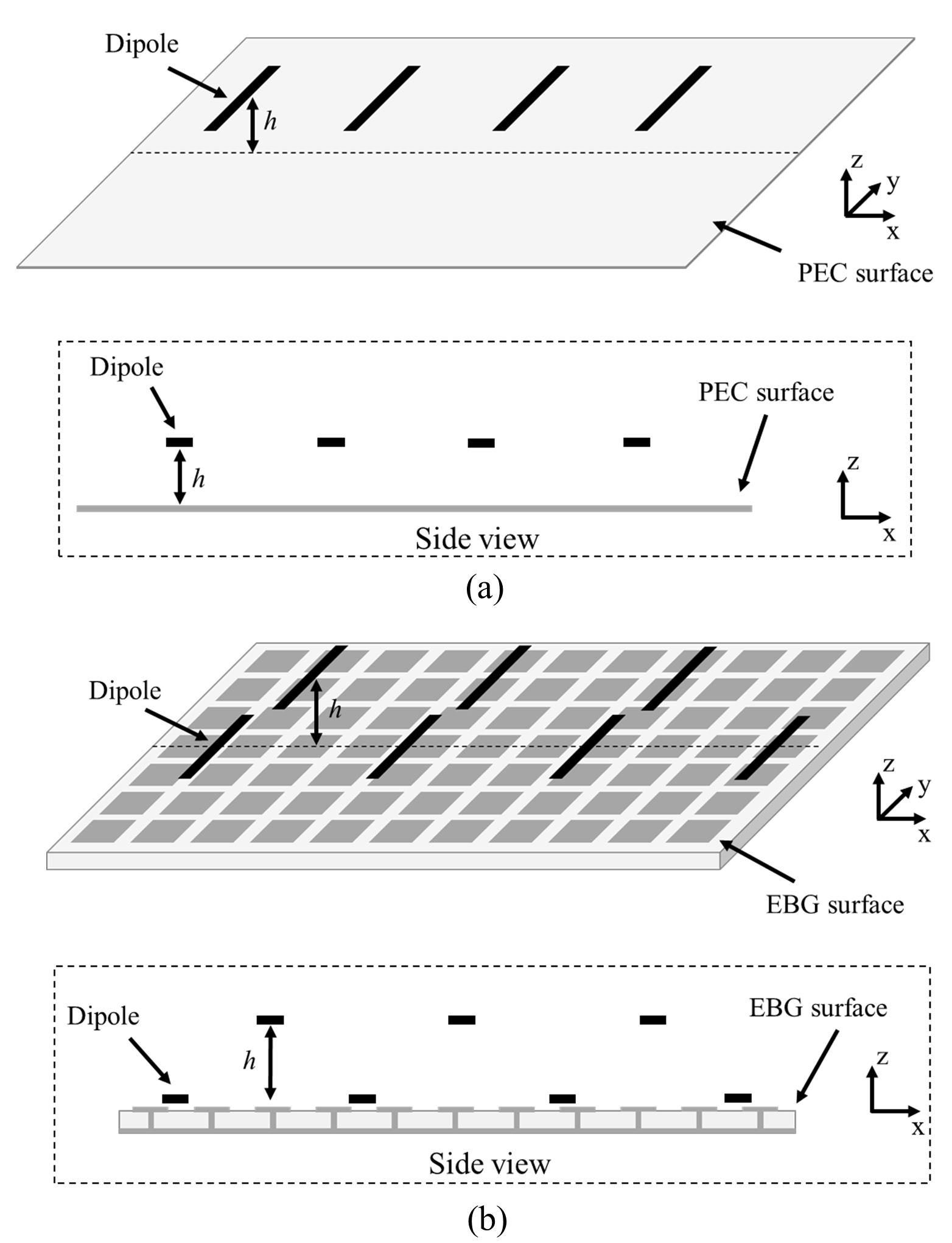
The diagrams of the traditional 2-D array topology and the proposed 3-D array topology are depicted in Fig. 1. Without loss of generality, a one-row array is set up along the -axis for reducing the complexities of analysis and design. Rather than using the traditional 2-D planar array with a perfect electric conductor (PEC) reflector in Fig. 1(a), a height difference is introduced between the nearby antennas for realizing the 3-D array in Fig. 1(b). The lower antennas are close to the EBG surface while the upper antennas maintain a suitable height difference, which can be enabled by a well-designed EBG surface. In 3-D array, the spatial differences between the array elements are not only along the transverse directions ( and directions), but also along the longitudinal direction ( direction).
Intuitively, the distance between the nearby antennas becomes larger because of the introduced height difference, and thus the spatial correlation between them will become lower (indicating a larger DOF) due to the fact that the spatial correlation between the antennas is usually negatively correlated to the distance between them.
From another perspective, the area of the oblique projection of 3-D array on the transverse plane is always larger than the area of the aperture of 2-D array. The above indicates that the additional volume along the vertical dimension can be utilized for realizing an equivalently larger 2-D array. Hence, the 3-D array shows the potential of breaking the DOF limit of a holographic MIMO system built with planar 2-D arrays. To further explore the properties of 3-D array, including the benefits and drawbacks, the 3-D Clarke and Kronecker models are first used for characterizing the MIMO performances, as discussed below.
2.1 3-D Clarke model
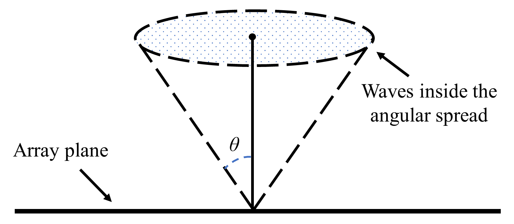
Based on the 3-D Clarke model [44, 45], the correlations between antennas in a Rayleigh fading environment can be analytically modeled for the theoretical analysis of MIMO performance. In the Clarke model, the antennas are simplified as point receivers, and the incident waves are modeled as uniformly distributed far-field plane waves. The angular spread of the incident waves can be modified for approximately characterizing different scattering environments, as the spatial correlation is dominated by the angular spread, but not the specific distribution of the incident waves [46]. An illustration of angular spread is depicted in Fig. 2, and the mean incident angle is taken along the broadside of the array. The total signal received by one antenna can be regarded as the integral of these received plane waves along solid angles (with sufficient number of plane waves). Therefore, one can easily formulate the correlation between the two antennas at the positions and by
| (1) |
where is the number of arriving plane waves, represent the solid angles of the plane waves within the angular spread, and denotes the wave vector along the direction. Then, the correlation matrix of the array can be obtained for evaluating the MIMO performance, i.e., the DOF and capacity.
To conveniently characterize the DOF performance (e.g., the limit and tendency) of a MIMO system, the diversity measure is used here [47, 48]. Diversity , which can approximately represent the equivalent number of isolated antennas of a MIMO array, can be calculated by [47]
| (2) |
where represents the trace operator and is the th eigenvalue of the correlation matrix . Furthermore, we evaluate the capacity of MIMO systems under the vertical-bell-labs-space-time (V-BLAST) architecture [2], where the transmitting side is ideal (the antennas are uncorrelated and their efficiencies are equal to 1). The channel matrix is unknown to the transmitters, and the transmitting power is equally allocated. This architecture allows us to focus on the characteristics of array at the receiving side. The ergodic capacity incorporating antenna effects can be written as [49]
| (3) |
where represents the mathematical expectation, H is the Hermitian operator, the covariance matrix equals to in the Clarke model (ideal antenna efficiencies), and is the identity matrix. Moreover, and are the number of transmitting and receiving antennas (), is the fixed total signal-to-noise ratio (SNR), and the entries of are independent and identically distributed (i.i.d.) complex Gaussian variables. The is normalized by making when the element spacing is larger than half wavelength, and making otherwise [17, 50], where is the number of antennas at element spacing.
2.2 Kronecker model
For practical antenna arrays, the deformation of radiation patterns and the decrease of radiation efficiencies caused by mutual coupling are required to be taken into consideration [51, 49, 52]. The covariance matrix is constructed by the entry-wise product between the correlation matrix and the embedded efficiency matrix , i.e.,
| (4) |
The correlation matrix incorporating mutual coupling is [53]
| (5) |
where
| (6) |
with
| (7) |
and are the and polarized embedded radiation patterns, is the angular power spectrum, and is the cross-polarization discrimination (XPD). The XPD is taken as 1 (polarization-balanced), and could be used for characterizing different angular spreads. The embedded efficiency matrix is
| (8) |
with
| (9) |
where the embedded radiation efficiency of the th antenna is calculated by the parameters assuming negligible ohmic loss [54]
| (10) |
3 Theoretical analysis
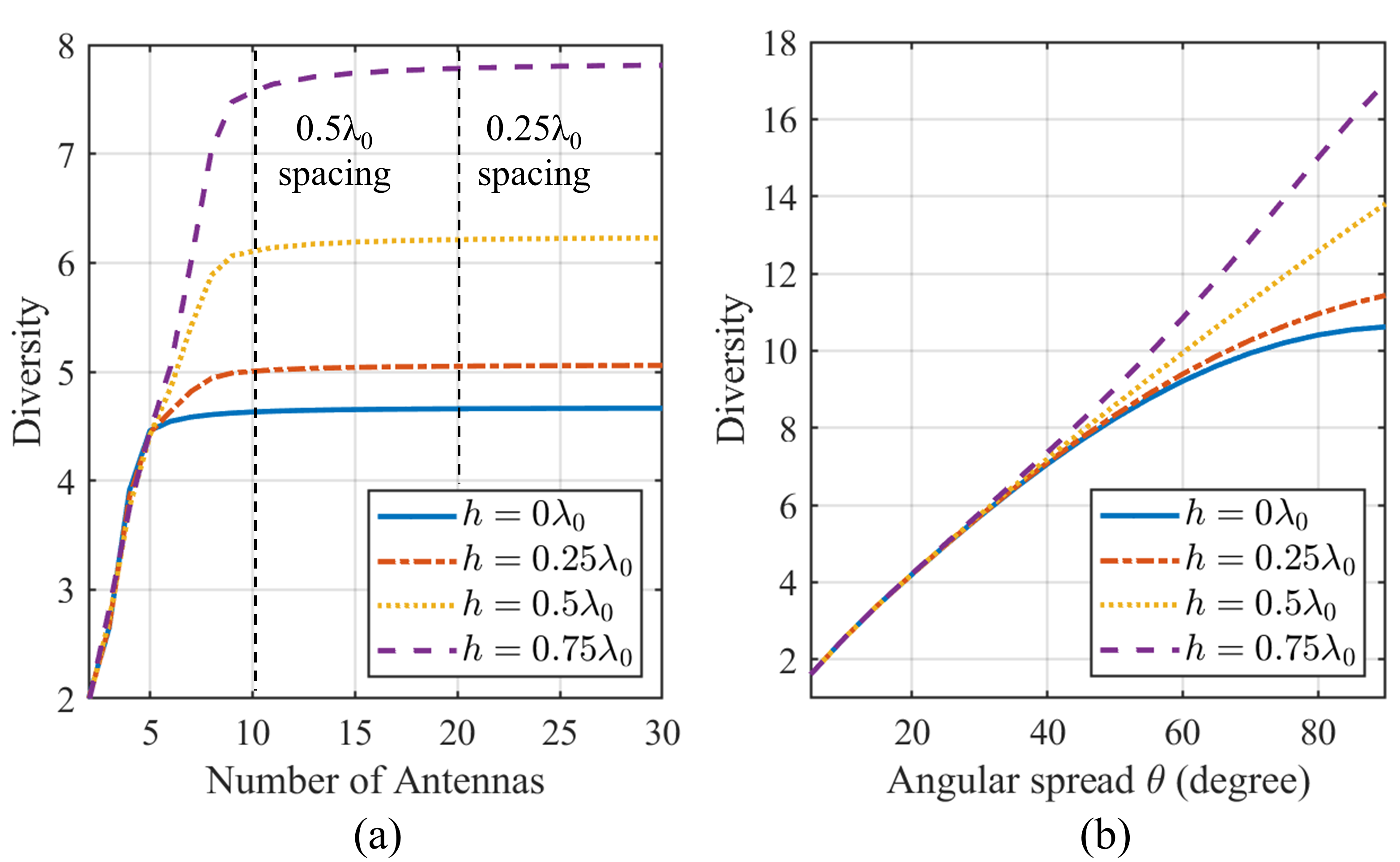
We commence with the foundational Clarke model, wherein antennas are approximated as isotropic point sources, and mutual couplings are disregarded. In this section, the lengths of all the arrays are fixed as 5, a height difference is introduced between the nearby antennas for realizing 3-D array (see Fig. 1), and the 3-D array will degenerate into 2-D array when . The diversities of 3-D arrays in different scenarios are investigated and presented in Fig. 3. In Fig. 3(a), it can be observed that the diversity in 2-D case () will not further increase when element spacing reaches nearly 0.5, which is the fundamental DOF limit of conventional holographic MIMO communications. However, the limit can be surpassed when a height difference between the nearby antennas is introduced, and the diversity keeps increasing until nearly 0.25 element spacing.
Moreover, the diversities under different angular spreads are presented in Fig. 3(b), where the increment of diversity brought by the 3-D configuration is positively related to the angular spread. It is reasonable that the benefit brought by the 3-D array will decrease at a small angular spread, since the projection of a 3-D array on the transverse plane will become close to that of a 2-D array at a small projection angle.
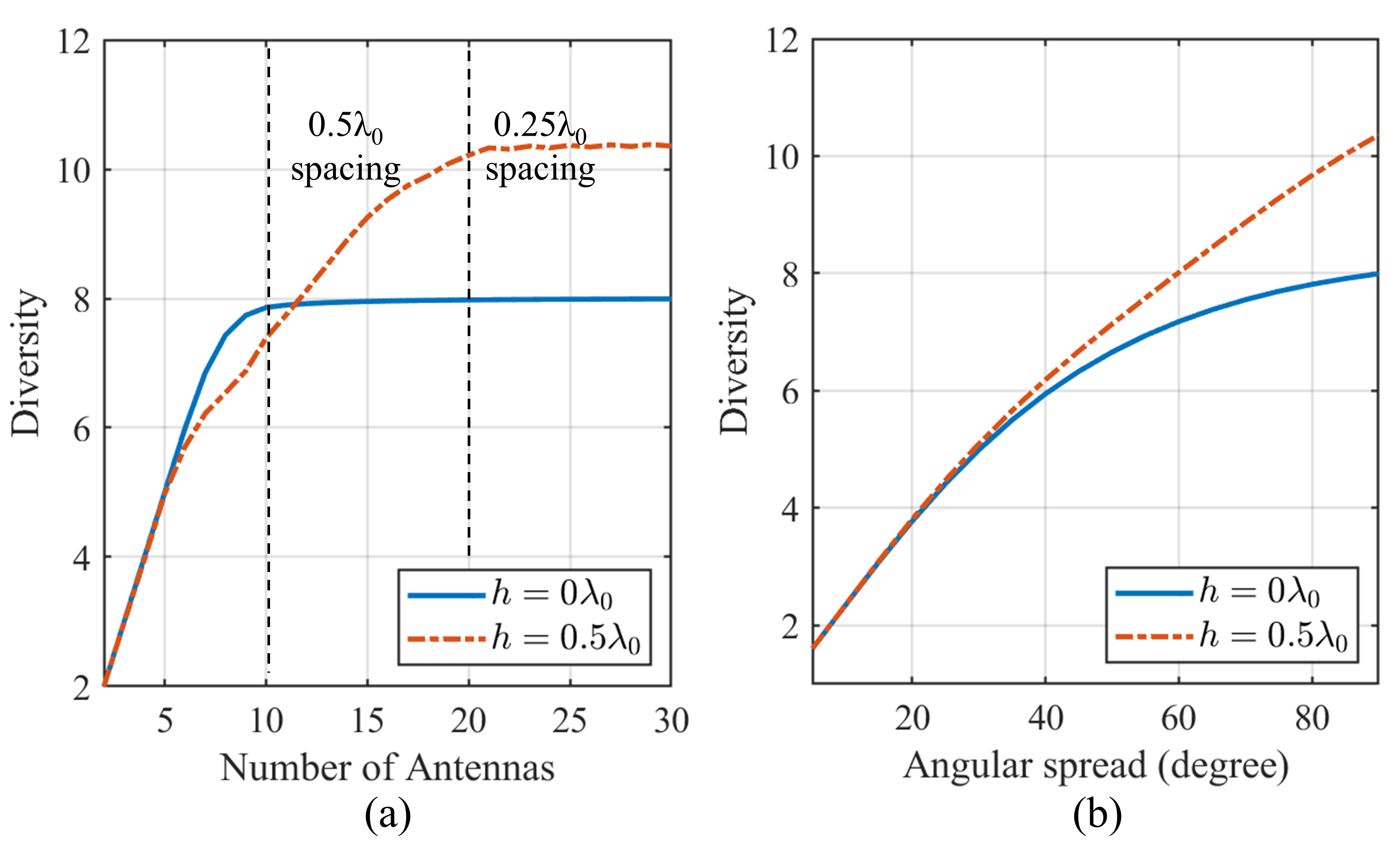
The Kronecker model can be used for taking into account the effects of antenna radiation patterns. Rather than using an isotropic radiation pattern for each antenna, the radiation patterns of the lower and upper antennas would be different, where the lower and upper antennas exhibit distinct radiation patterns from isolated antennas. In practical designs, side lobes are almost unavoidable when the height difference is large according to the antenna array theory [32], and a 0.5 height difference is taken here for balancing the antenna performance and benefits. The isolated radiation patterns of two practical antennas are exported for performing the theoretical analyses here, including the lower antenna close to the EBG surface and the upper antenna 0.5 higher than the EBG surface. The corresponding antenna designs and radiation patterns are demonstrated in Fig. 7(b-c) and Fig. 10(a-b).
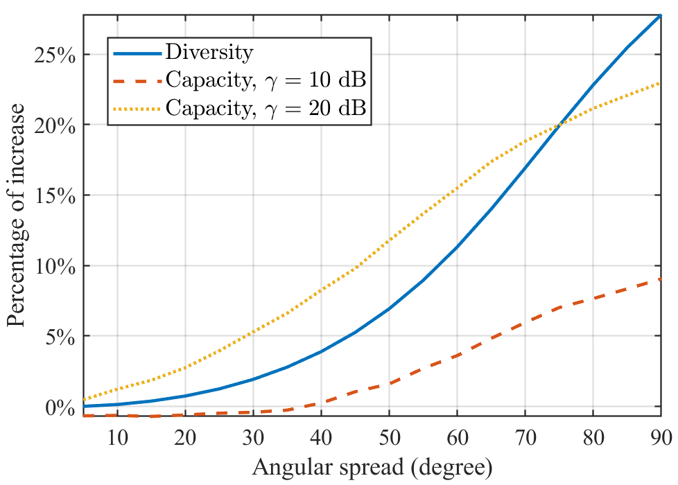
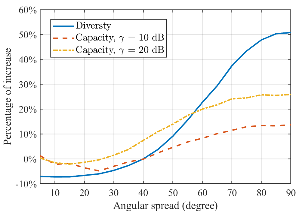
Based on the Kronecker model, the diversities of 3-D arrays are calculated and presented in Fig. 4, showing that the DOF limit can be broken by using the 3-D configuration, and the increment brought by the 3-D array is largely dependent on the angular spread. For a better illustration, we plot the percentage of increases of diversity and capacity brought by the 3-D array compared to the 2-D array with the same aperture size in Fig. 5. Theoretically, i.e., ideal decouplings are made, the diversity can be increased by , and the capacity can be increased by ( dB) and ( dB) in an isotropic multi-path environment (angular spread is . In practical applications, the angular spread may become smaller. When the angular spread is , the diversity can still be increased by , and the capacity can be increased by ( dB) and ( dB). Hence, the theoretical analyses put forth in this study strongly suggest that the proposed 3-D configuration successfully transcends the DOF limit, showcasing its potential application for enhancing capacity across a multitude of scenarios.
4 Numerical and experimental verifications
4.1 Design of the 3-D array
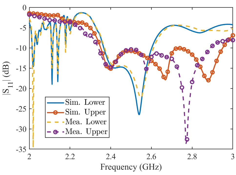
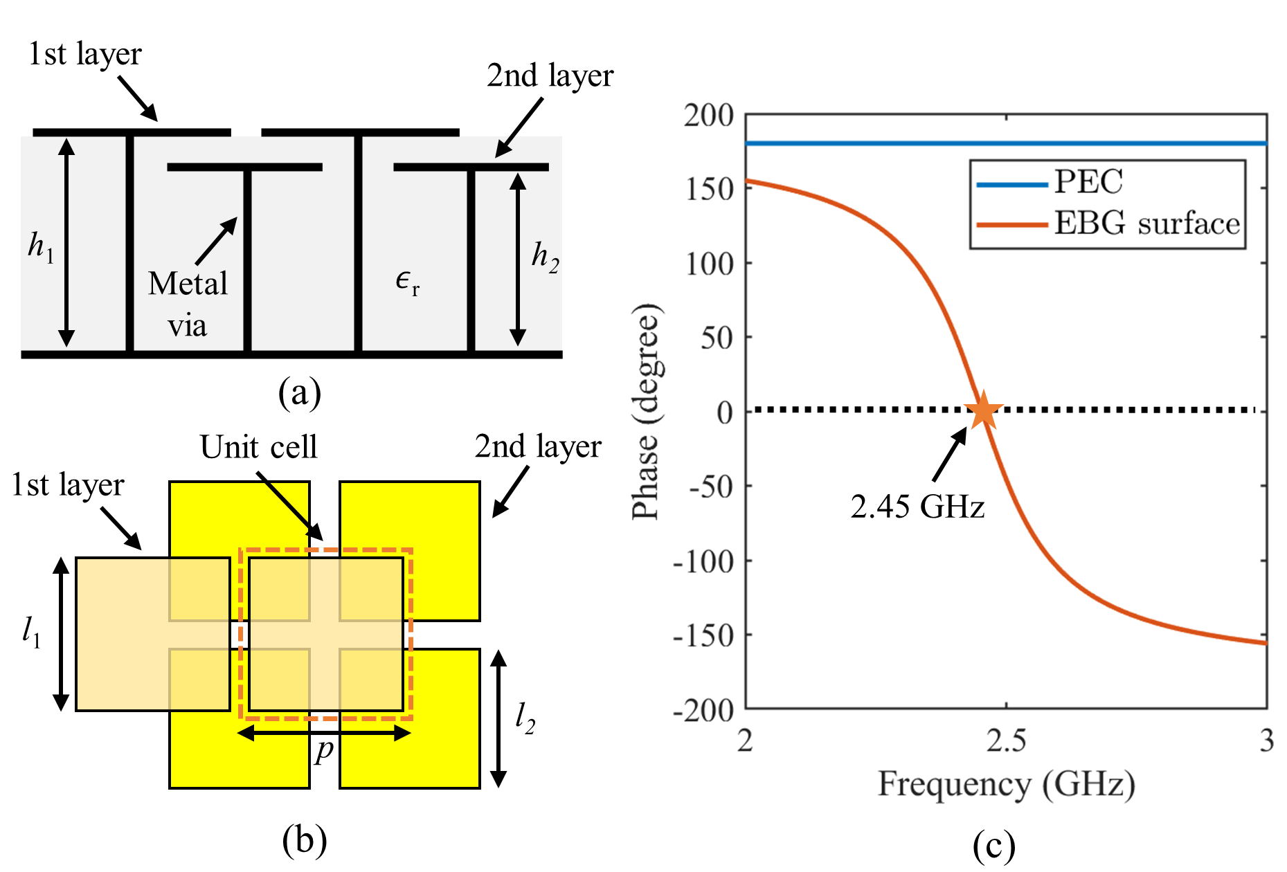
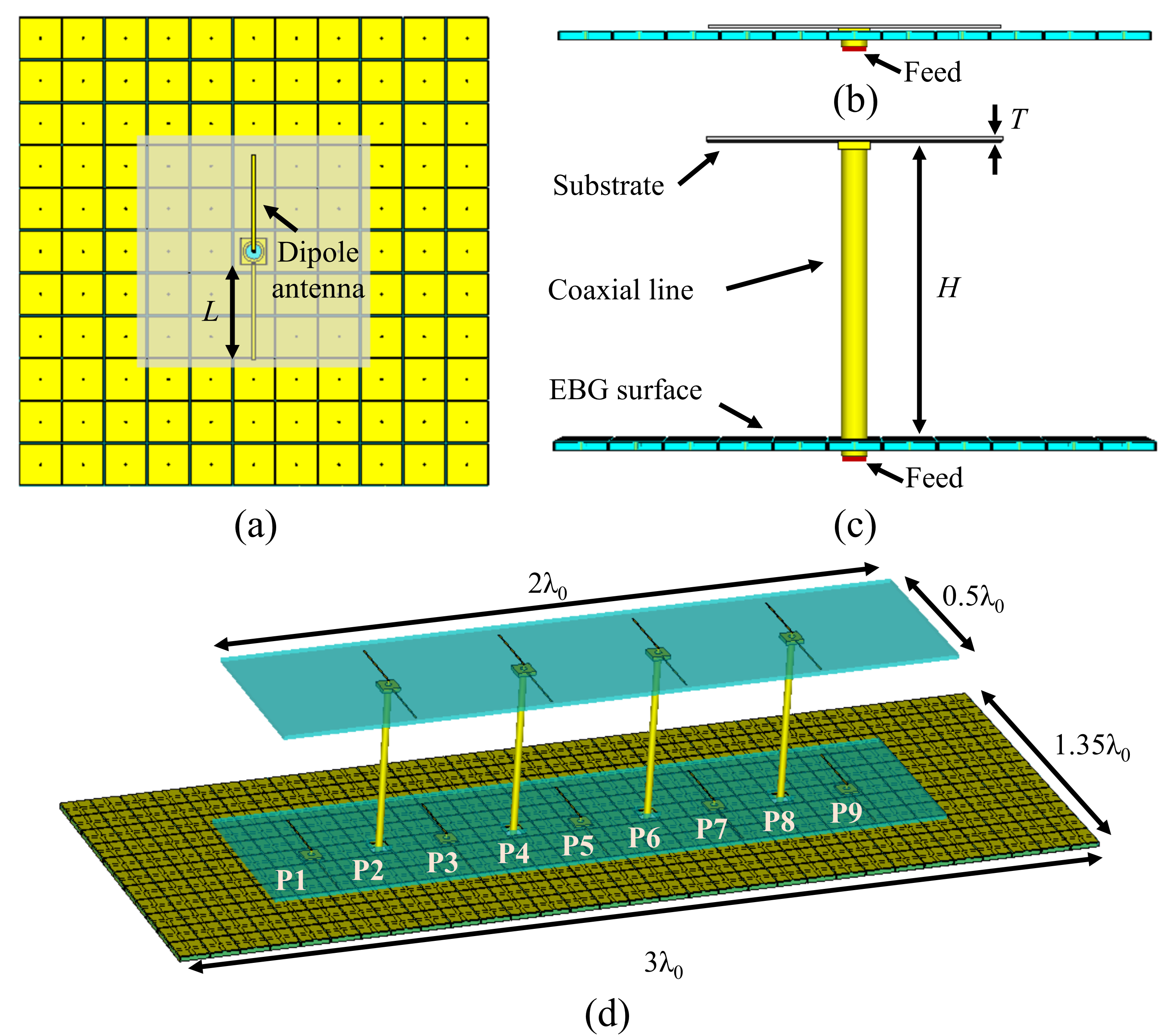
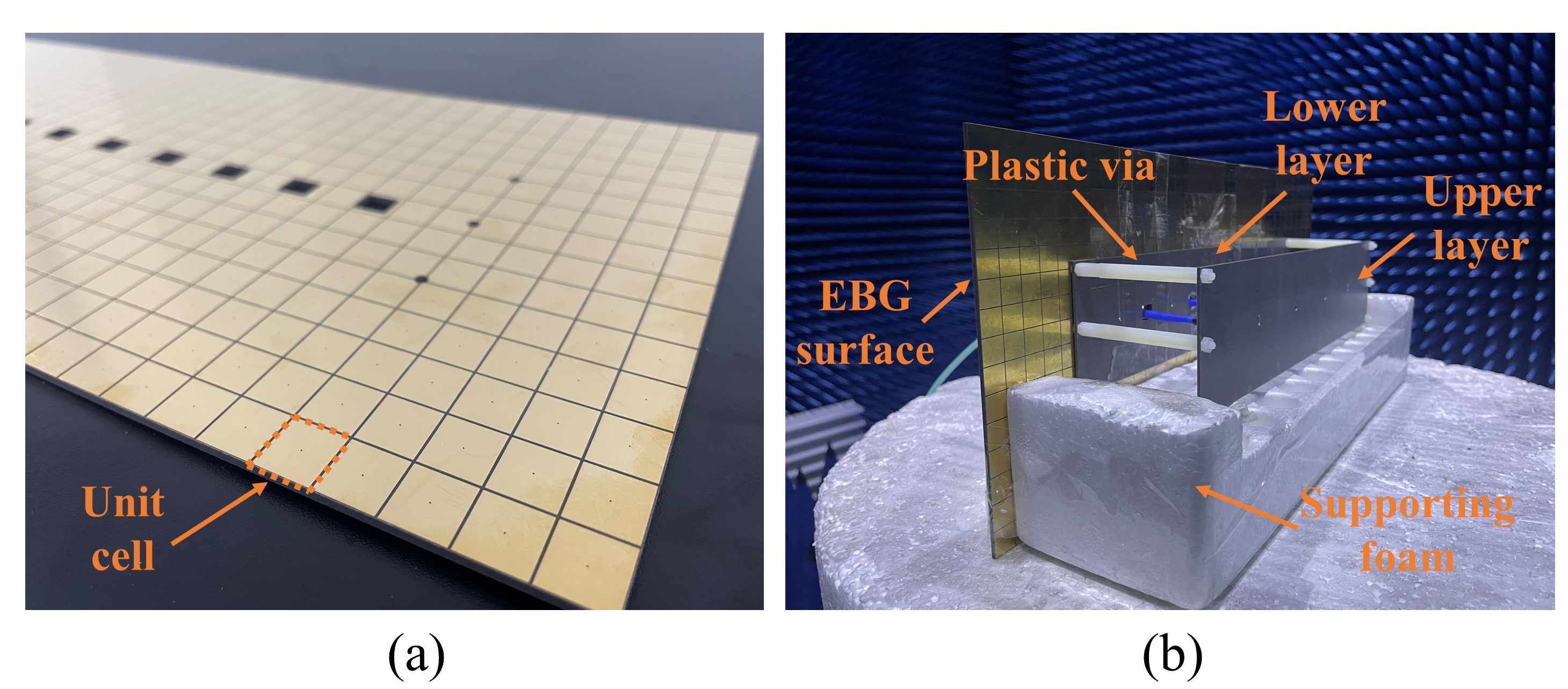
As a proof of concept, a practical 3-D array enabled by an EBG surface is designed for verifying the above theoretical analyses. To create the 0.5 height difference while maintain acceptable antenna performances, a reflecting phase should be introduced by using the EBG surface at the working frequency. The design of EBG surfaces has been well discussed in literatures [55], and a double-layer EBG surface is used here for realizing the desired functions [56]. The diagram of the utilized EBG structure is plotted in Fig. 6(a-b), and a reflecting phase can be realized at 2.45 GHz in Fig. 6(c). To reduce the complexities of design, simulation and fabrication, a microstrip dipole antenna is used here for facilitating the procedure of verification, as shown in Fig. 7(a). The full-wave models of the isolated upper and lower antennas are presented in Fig. 7(a-c), and a perspective view of the constructed 3-D array can be found in Fig. 7(d). Furthermore, the proposed 3-D array in Fig. 7(d) is fabricated and fully measured, the fabricated samples and experimental setup are demonstrated in Fig. 8.
4.2 Numerical and experimental results of the 3-D array
4.2.1 Isolated antenna
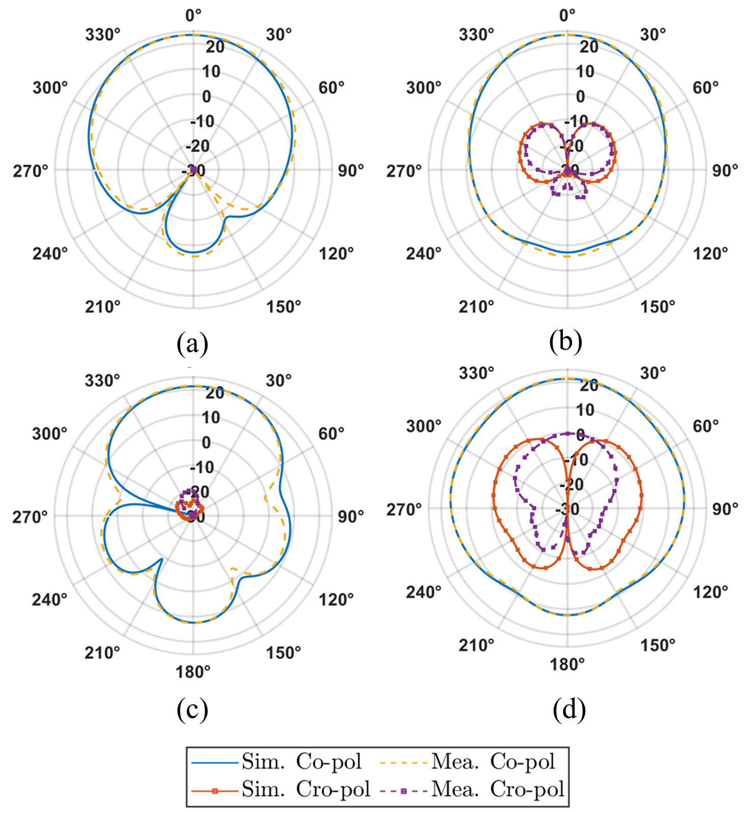
The reflection coefficients and far-field radiation patterns of the two isolated antennas, i.e., the lower and upper antennas presented in Fig. 7(b-c), are first investigated. Moreover, the electric-field patterns of the isolated antennas at far field (reference distance is taken as 1 m) are demonstrated in Fig. 10. It can be observed that the lower antenna maintains a regular radiation pattern [57], while the upper antenna has side lobes due to the introduced 0.5 height difference. The side lobes in the upper antenna are almost inevitable, since its radiation pattern can be regarded as the end-fire radiation of a two-element in-phase array with 1 distance. The performance of antennas in 3-D array can be further improved by antenna and decoupling designs.
4.2.2 Antennas in the 3-D array
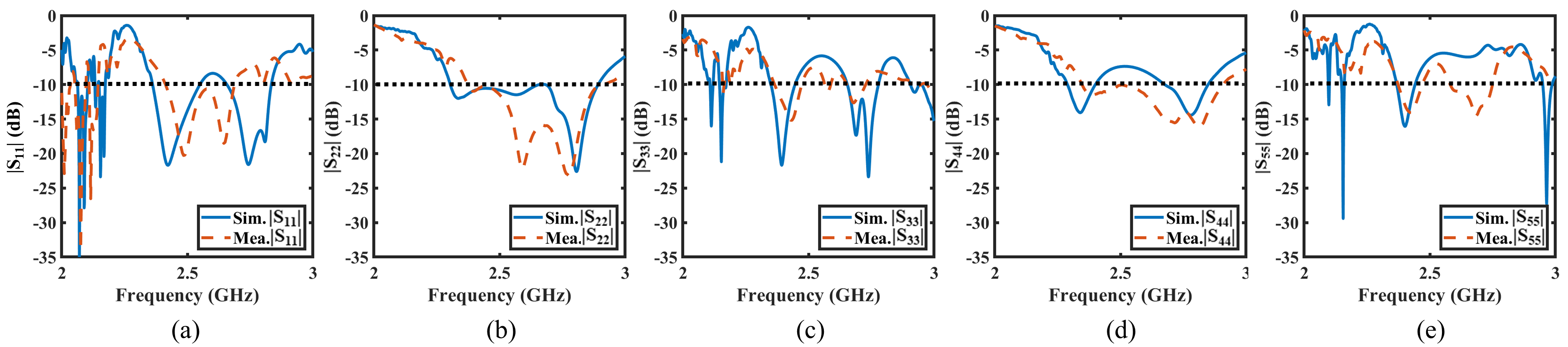
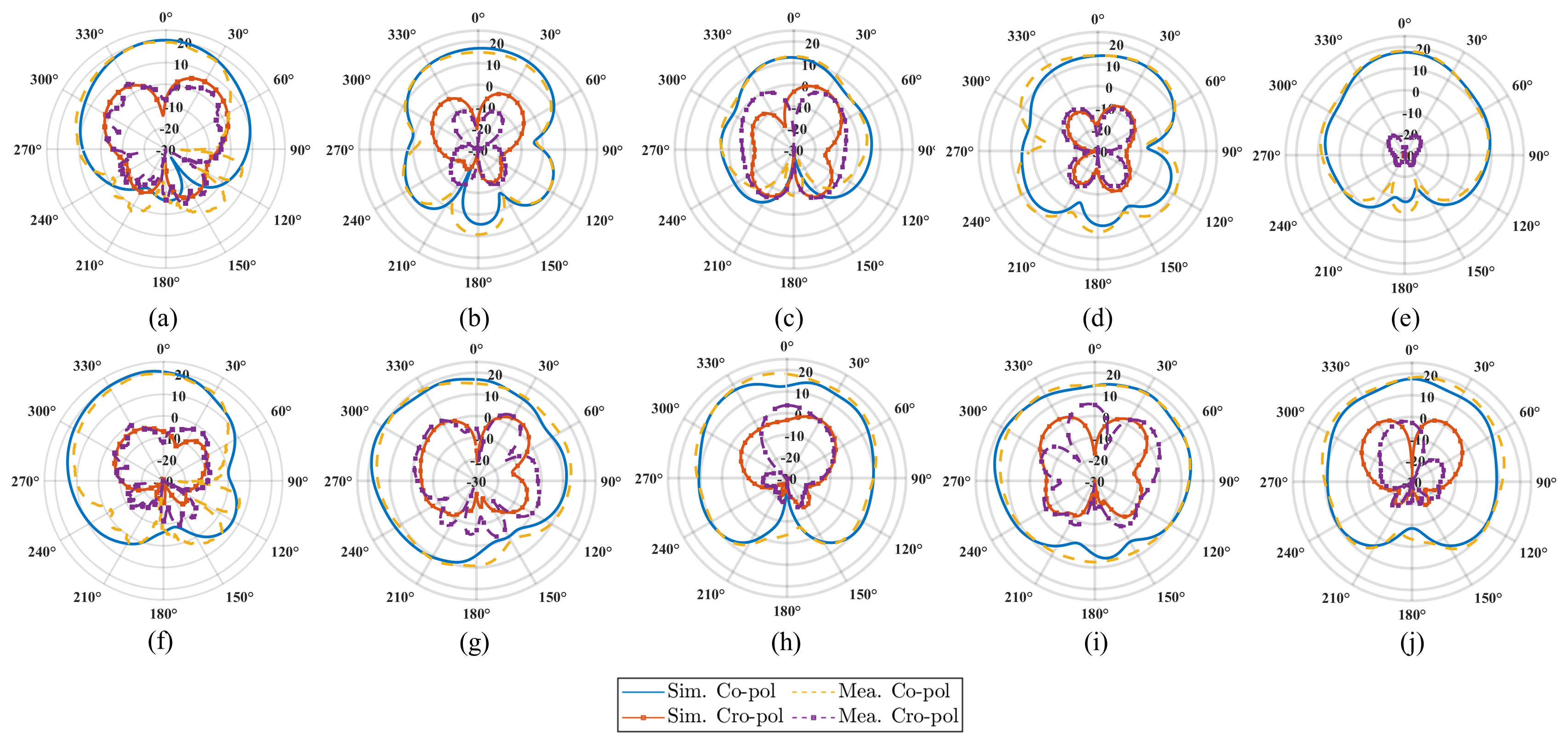
The parameters and embedded radiation patterns of the antennas in a practical 3-D array are simulated and measured. Specifically, the embedded radiation pattern of one antenna in the array is obtained by exciting this antenna while making all the other antennas well-matched. The results of the first five antennas, i.e., P1-P5 in Fig. 7(d), are given considering the symmetric structure of 3-D array. The simulated and measured reflection coefficients are plotted and compared in Fig. 11, some deviations can be attributed to the fabrication and measurement errors. In Fig. 12, the simulated and measured embedded radiation patterns of the antennas in 3-D array are given, where the shapes of radiation patterns are inevitably deformed due to the mutual coupling at small element spacing.
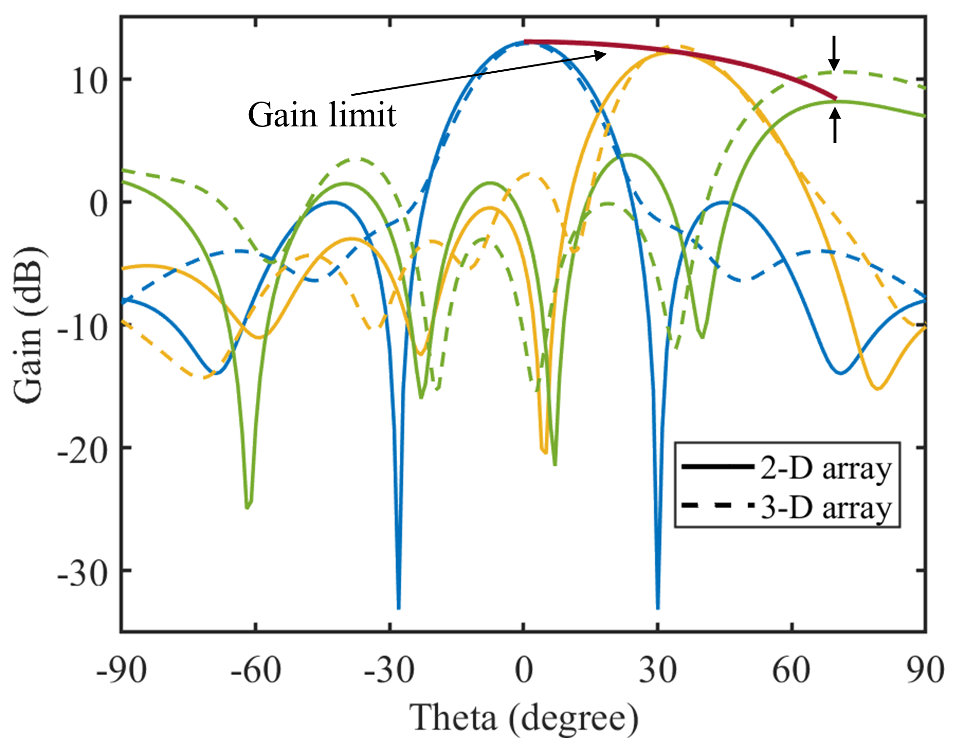
From the perspective of beamforming, the 3-D array will have better gain than the 2-D array especially at large scanning angles, because the corresponding projection area is larger. The gain limit of a 2-D array is given by [32]
| (11) |
where is the area of array, and represents the decrease of projection area due to the increase of . The 3-D array is expected to have larger projection area especially at large scanning angles benefiting from the increased height, thus breaks the gain limit of 2-D array at large angles, as shown in Fig. 13.
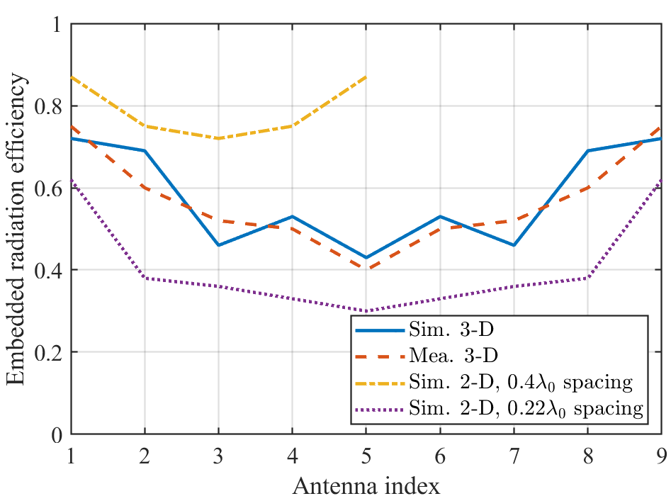
The embedded radiation efficiencies of the antennas are calculated from parameters according to (10), which are drawn and compared to the efficiencies in the 2-D arrays at different element spacings (i.e., different antenna numbers) in Fig. 14. It can be found that the efficiencies in the 3-D array are generally lower than that in the 2-D array at 0.4 spacing, but higher than that in the 2-D array at 0.22 spacing (with the same antenna number as the 3-D array). The latter indicates that the Hannan’s efficiency limit for a planar array [33] is in fact broken by introducing the height difference in the 3-D array.
4.3 MIMO performance
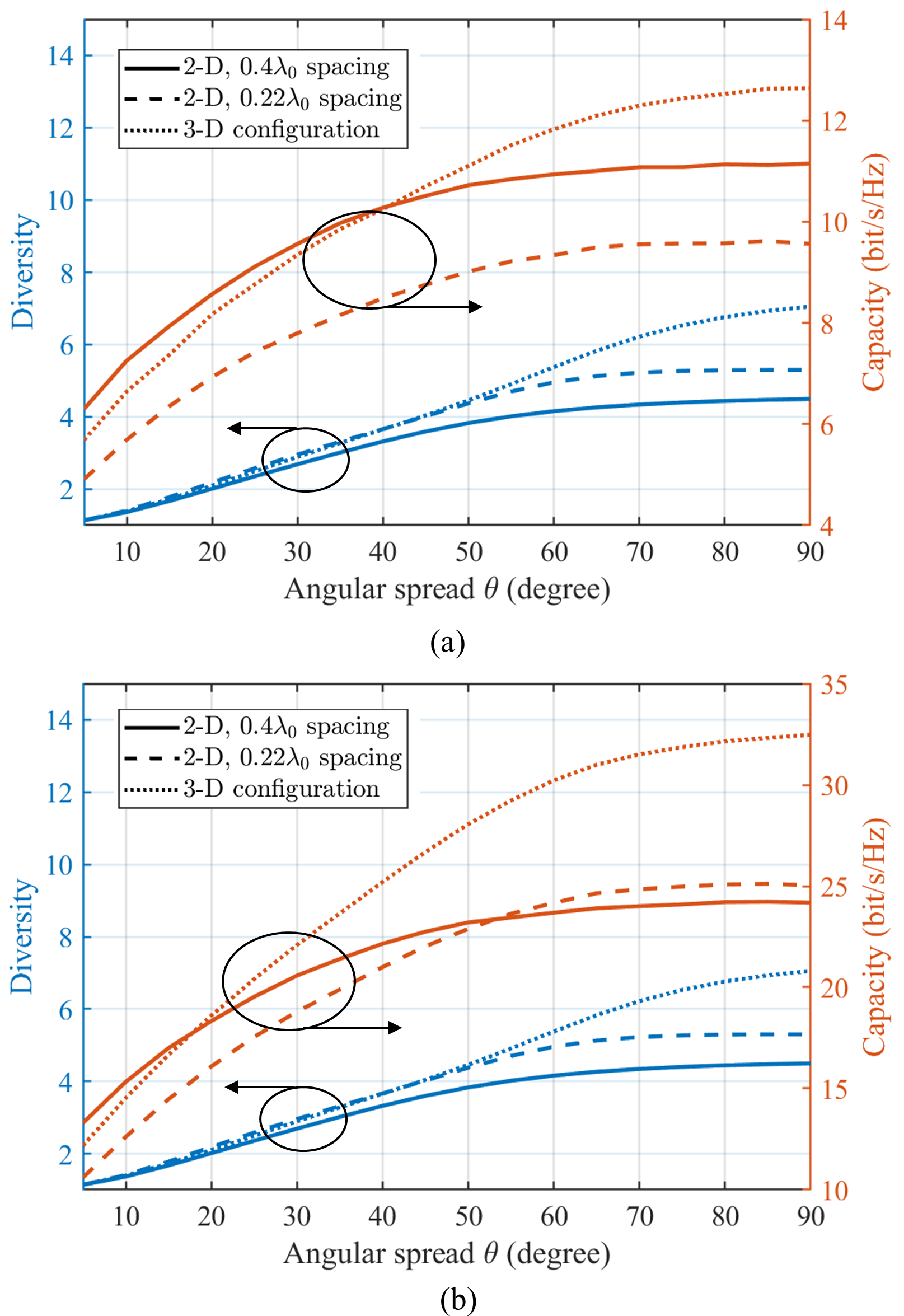
4.3.1 2 array in Rayleigh channel
With the above results, i.e., embedded radiation patterns and efficiencies, the diversity and capacity of 3-D array can be calculated and compared to the 2-D arrays with the same aperture size by using (3-10). Three types of arrays with 2 array length are first considered, including the proposed 3-D array, the 2-D array at 0.4 element spacing (i.e., only the lower layer of 3-D array), and the 2-D array at 0.22 element spacing (with the same antenna number as the 3-D array). The results at different SNR levels ( 10 and 20 dB) are depicted in Fig. 15(a) and Fig. 15(b), where the increments of diversities and capacities are close to the theoretical analyses in Section III. To be specific, compared to the 2-D array, the diversity is increased by , and the capacity is increased by ( 10 dB) and ( 20 dB) in isotropic multi-path environment. When the angular spread is , the diversity is increased by , and the capacity is increased by ( 10 dB) and ( 20 dB). Particularly, for a regular 2-D array, the diversity may only slightly increase due to the mutual coupling after reaching the DOF limit, but the efficiency will dramatically decrease following the Hannan’s limit [33]. Therefore, placing too many antennas into a constrained planar area will generally be harmful to capacity, as shown by the 0.22 and 0.4 spacing 2-D arrays in Fig. 15(a).
4.3.2 5 array in Rayleigh channel
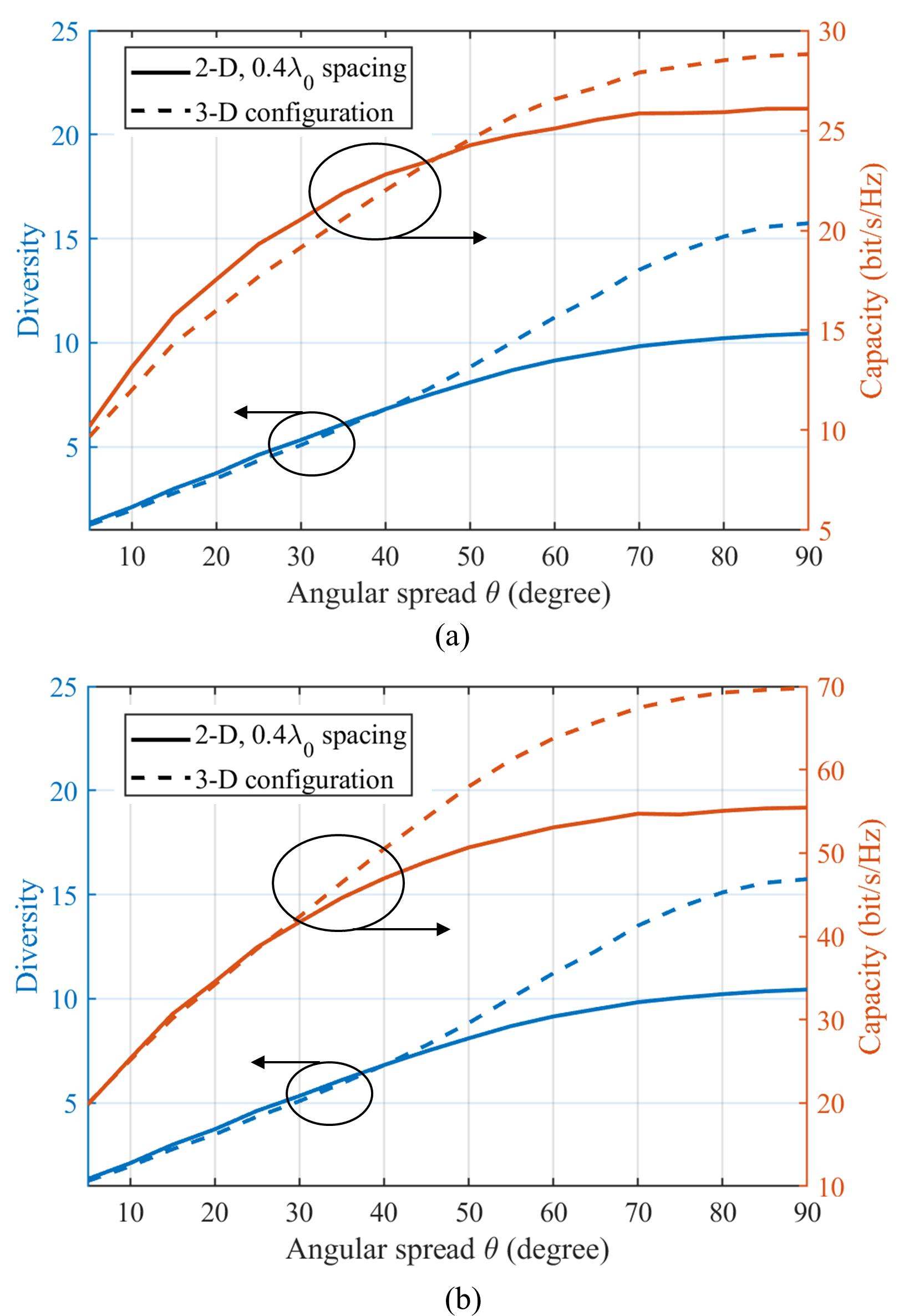
We also investigate the performance of a larger 3-D array in Fig. 16, with the length of 5 along the axis. In a large-scale array, the radiation patterns of the antennas in the middle region are similar [58], and the effect of edge antennas is usually small. Compared to the 2-D array at 0.4 spacing, the capacity is increased by ( 10 dB) and ( 20 dB) in isotropic multi-path environment, and increased by ( 10 dB) and ( 20 dB) when the angular spread is . In order to analyze the effects of mutual coupling, the percent of increase is drawn in Fig. 17 similar to the theoretical analysis in Fig. 5. It can be observed that the increments of capacities are slightly larger than the theoretical analyses in Section III at large angular spreads, because the large-angle radiations are stronger (indicating more DOF benefits are brought by the 3-D array configuration). However, the radiation efficiencies are considerably decreased by mutual coupling, which will degrade the performance of 3-D array at low SNR and small angular spreads (the capacity enhancement brought by the extra DOF is not significant). Therefore, the benefit of 3-D array is highly dependent on the SNR level, specific multi-path environments and antenna designs (radiation patterns), and the obtained results reveal the superiorities of 3-D array over the 2-D array with the same aperture size in many scenarios.
4.3.3 3GPP channel
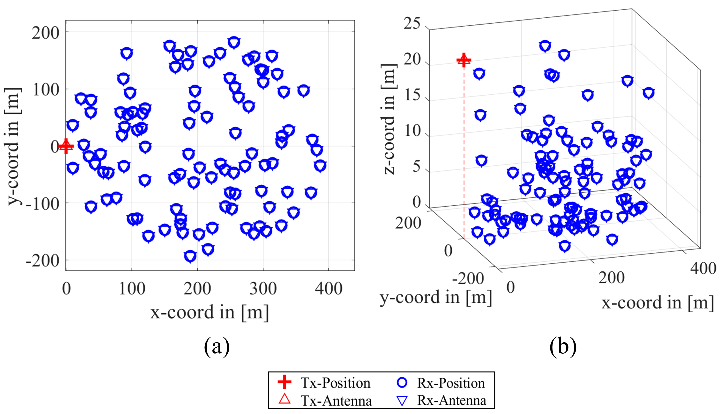
To further investigate the MIMO performances of the 3-D array in practical communication environments rather than in the ideal Rayleigh channel, the open-source software QuaDRiGa is used for comparing the performances of 2-D and 3-D arrays in 3GPP channels [59]. Particularly, two single-cell scenarios are considered, including the 2-D 3GPP urban macro (UMa) and 3-D 3GPP UMa scenarios [59]. The configurations of the 3GPP models are demonstrated in Fig. 18, where the users (marked by blue circles) are distributed in a circular area with the radius of 200 m, and the base station (marked by red cross) is placed at the left side of the circular area with the height of 25 m.
The users are arranged in accordance with the 3GPP assumptions[60], where 80 of them are situated indoors at different floor levels for the 3-D scenario and all set outdoors (1.5 m height) for the 2-D scenario. The embedded radiation patterns of the proposed 2 3-D array are imported as transmitting array, while the users are set as omnidirectional antennas. Then, the channels of the paths created by different clusters are generated and summed for obtaining the wanted channel matrix. Following (2-10), the diversity and capacity can be obtained for investigating the properties of 3-D array in geometry-based spatial correlation channels. The diversities and capacities ( = 20 dB) with different numbers of users are calculated 20 times and averaged (each time the users are at different random positions), as presented in Table I. Compared to using the 2-D array with the same aperture size, the capacity can be increased by nearly 10 with 3-D array. Obviously, the benefits brought by the 3-D array in 3GPP channel are smaller than that in Rayleigh channel because of the smaller angular spread at the base station in 3GPP channels. Specifically, the azimuth angle spread at the base station side is regulated to be smaller than 104∘ (angular spread 52∘) according to 3GPP TR 38.901 [60]. Therefore, when implementing 3-D array, the specific settings should be carefully taken into consideration, including the array design, multi-path environment, SNR level, user density, etc.
| Scenarios | 2-D array | 3-D array | Percent of increase | ||
|---|---|---|---|---|---|
|
1.83 | 2.18 | 16% | ||
|
18.50 | 21.08 | 13% | ||
|
2.56 | 3.01 | 17% | ||
|
21.13 | 23.80 | 13% | ||
|
1.65 | 1.79 | 8% | ||
|
16.84 | 18.17 | 8% | ||
|
1.80 | 1.99 | 11% | ||
|
17.76 | 19.02 | 7% |
5 Conclusion
In this study, we successfully overcome the fundamental DOF limit in holographic MIMO communications by introducing a 3-D array topology. We systematically elucidate the principles behind the DOF limit and demonstrate the step-by-step utilization of the 3-D array topology to surpass this constraint, progressing from the ideal Clarke model to practical scenarios. Particularly, the benefits of 3-D array are illustrated from the perspectives of electromagnetics and beamforming. The numerical and experimental results further substantiate that, after reaching the DOF limit, the diversities and capacities of MIMO systems can be further improved by applying the 3-D topology. Furthermore, the performances of 3-D array in 3GPP channels are investigated, regarding the possible small angular spreads in practical implementations. Consequently, the 3-D array stands out as a promising candidate for bolstering MIMO performance across various scenarios in the future landscape of wireless communications.
Future endeavors will delve into exploring corresponding channel modeling and precoding technologies. Additionally, we aim to enhance hardware designs, incorporating advanced antenna and decoupling structures to improve radiation patterns and matchings. These avenues of research will contribute to the ongoing advancement and optimization of holographic MIMO communication systems.
References
- [1] Emre Telatar. Capacity of multi-antenna Gaussian channels. Eur. Trans. Telecomm., 10(6):585–595, 1999.
- [2] David Tse and Pramod Viswanath. Fundamentals of wireless communication. 2005.
- [3] Arogyaswami J Paulraj, Dhananjay A Gore, Rohit U Nabar, and Helmut Bolcskei. An overview of MIMO communications-a key to gigabit wireless. Proc. IEEE, 92(2):198–218, 2004.
- [4] Erik G. Larsson, Ove Edfors, Fredrik Tufvesson, and Thomas L. Marzetta. Massive MIMO for next generation wireless systems. IEEE Commun. Mag., 52(2):186–195, 2014.
- [5] Emil Björnson, Luca Sanguinetti, Henk Wymeersch, Jakob Hoydis, and Thomas L Marzetta. Massive MIMO is a reality—what is next?: Five promising research directions for antenna arrays. Digit. Signal Prog., 94:3–20, 2019.
- [6] Jakob Hoydis, Stephan ten Brink, and Merouane Debbah. Massive MIMO in the UL/DL of cellular networks: How many antennas do we need? IEEE J. Sel. Areas Commun., 31(2):160–171, 2013.
- [7] Zhe Wang, Jiayi Zhang, Hongyang Du, Wei E. I. Sha, Bo Ai, Dusit Niyato, and Merouane Debbah. Extremely large-scale MIMO: Fundamentals, challenges, solutions, and future directions. IEEE Wirel. Commun., pages 1–9, 2023.
- [8] Ke-Li Wu, Changning Wei, Xide Mei, and Zhen-Yuan Zhang. Array-antenna decoupling surface. IEEE Trans. Antennas Propag., 65(12):6728–6738, 2017.
- [9] Shuai Zhang, Xiaoming Chen, and Gert Frølund Pedersen. Mutual coupling suppression with decoupling ground for massive MIMO antenna arrays. IEEE Trans. Veh. Technol., 68(8):7273–7282, 2019.
- [10] Xiaoming Chen, Mengran Zhao, Huilin Huang, Yipeng Wang, Shitao Zhu, Chao Zhang, Jianjia Yi, and Ahmed A Kishk. Simultaneous decoupling and decorrelation scheme of MIMO arrays. IEEE Trans. Veh. Technol., 71(2):2164–2169, 2021.
- [11] Yipeng Wang, Xiaoming Chen, Xiaobo Liu, Jianjia Yi, Juan Chen, Anxue Zhang, and Ahmed A Kishk. Improvement of diversity and capacity of MIMO system using scatterer array. IEEE Trans. Antennas Propag., 70(1):789–794, 2021.
- [12] Wankai Tang, Jun Yan Dai, Ming Zheng Chen, Kai-Kit Wong, Xiao Li, Xinsheng Zhao, Shi Jin, Qiang Cheng, and Tie Jun Cui. MIMO transmission through reconfigurable intelligent surface: System design, analysis, and implementation. IEEE J. Sel. Areas Commun., 38(11):2683–2699, 2020.
- [13] Chongwen Huang, Alessio Zappone, George C. Alexandropoulos, Mérouane Debbah, and Chau Yuen. Reconfigurable intelligent surfaces for energy efficiency in wireless communication. IEEE Trans. Wirel. Commun., 18(8):4157–4170, 2019.
- [14] Li Wei, Chongwen Huang, George C Alexandropoulos, Wei E. I. Sha, Zhaoyang Zhang, Mérouane Debbah, and Chau Yuen. Multi-user holographic MIMO surfaces: Channel modeling and spectral efficiency analysis. IEEE J. Sel. Top. Signal Process., 16(5):1112–1124, 2022.
- [15] Jiancheng An, Chao Xu, Derrick Wing Kwan Ng, George C. Alexandropoulos, Chongwen Huang, Chau Yuen, and Lajos Hanzo. Stacked intelligent metasurfaces for efficient holographic MIMO communications in 6g. IEEE J. Sel. Areas Commun., 41(8):2380–2396, 2023.
- [16] Li Wei, Chongwen Huang, George C. Alexandropoulos, Zhaohui Yang, Jun Yang, Wei E. I. Sha, Zhaoyang Zhang, Mérouane Debbah, and Chau Yuen. Tri-polarized holographic MIMO surfaces for near-field communications: Channel modeling and precoding design. IEEE Trans. Wirel. Commun., pages 1–1, 2023.
- [17] Shuai S. A. Yuan, Xiaoming Chen, Chongwen Huang, and Wei E. I. Sha. Effects of mutual coupling on degree of freedom and antenna efficiency in holographic MIMO communications. IEEE Open J. Antennas Propag., 4:237–244, 2023.
- [18] Yuan Zhang, Jianhua Zhang, Yuxiang Zhang, Yuan Yao, and Guangyi Liu. Capacity analysis of holographic MIMO channels with practical constraints. IEEE Wireless Commun. Lett., 12(6):1101–1105, 2023.
- [19] Ozlem Tugfe Demir, Emil Bjornson, and Luca Sanguinetti. Channel modeling and channel estimation for holographic massive MIMO with planar arrays. IEEE Wireless Commun. Lett., 11(5):997–1001, 2022.
- [20] Andrea Pizzo, Thomas L. Marzetta, and Luca Sanguinetti. Spatially-stationary model for holographic MIMO small-scale fading. IEEE J. Sel. Areas Commun., 38(9):1964–1979, 2020.
- [21] Chongwen Huang, Sha Hu, George C. Alexandropoulos, Alessio Zappone, Chau Yuen, Rui Zhang, Marco Di Renzo, and Merouane Debbah. Holographic mimo surfaces for 6g wireless networks: Opportunities, challenges, and trends. IEEE Wirel. Commun., 27(5):118–125, 2020.
- [22] Andrea Pizzo, Thomas L. Marzetta, and Luca Sanguinetti. Degrees of freedom of holographic MIMO channels. In 2020 IEEE 21st International Workshop on Signal Processing Advances in Wireless Communications (SPAWC), pages 1–5, 2020.
- [23] George C. Alexandropoulos, P. Takis Mathiopoulos, and Nikos C. Sagias. Switch-and-examine diversity over arbitrarily correlated nakagami- fading channels. IEEE Trans. Veh. Technol., 59(4):2080–2087, 2010.
- [24] Marco Donald Migliore. Horse (electromagnetics) is more important than horseman (information) for wireless transmission. IEEE Trans. Antennas Propag., 67(4):2046–2055, 2019.
- [25] Shuai S. A. Yuan, Zi He, Xiaoming Chen, Chongwen Huang, and Wei E. I. Sha. Electromagnetic effective degree of freedom of an MIMO system in free space. IEEE Antennas Wirel. Propag. Lett., 21(3):446–450, 2022.
- [26] Zhongzhichao Wan, Jieao Zhu, Zijian Zhang, Linglong Dai, and Chan-Byoung Chae. Mutual information for electromagnetic information theory based on random fields. IEEE Trans Commun., 71(4):1982–1996, 2023.
- [27] Zixiang Han, Shanpu Shen, Yujie Zhang, Shiwen Tang, Chi-Yuk Chiu, and Ross Murch. Using loaded n-port structures to achieve the continuous-space electromagnetic channel capacity bound. IEEE Trans. Wirel. Commun., pages 1–1, 2023.
- [28] Wonseok Jeon and Sae-Young Chung. Capacity of continuous-space electromagnetic channels with lossy transceivers. IEEE Trans. Inf. Theory, 64(3):1977–1991, 2018.
- [29] Massimo Franceschetti. Wave Theory of Information. Cambridge University Press, 2017.
- [30] Mats Gustafsson and Johan Lundgren. Degrees of freedom and characteristic modes. 2023.
- [31] Davide Dardari and Nicolò Decarli. Holographic communication using intelligent surfaces. IEEE Commun. Mag., 59(6):35–41, 2021.
- [32] Constantine A Balanis. Antenna theory: analysis and design. 2015.
- [33] P. Hannan. The element-gain paradox for a phased-array antenna. IEEE Trans. Antennas Propag., 12(4):423–433, 1964.
- [34] O.M. Bucci and G. Franceschetti. On the degrees of freedom of scattered fields. IEEE Trans. Antennas Propag., 37(7):918–926, 1989.
- [35] Shuai S. A. Yuan, Jie Wu, Menglin L. N. Chen, Zhihao Lan, Liang Zhang, Sheng Sun, Zhixiang Huang, Xiaoming Chen, Shilie Zheng, Li Jun Jiang, Xianmin Zhang, and Wei E. I. Sha. Approaching the fundamental limit of orbital-angular-momentum multiplexing through a hologram metasurface. Phys. Rev. Applied, 16:064042, 2021.
- [36] Casimir Ehrenborg, Mats Gustafsson, and Miloslav Capek. Capacity bounds and degrees of freedom for MIMO antennas constrained by Q-factor. IEEE Trans. Antennas Propag., 69(9):5388–5400, 2021.
- [37] Michael A. Jensen and Jon W. Wallace. Capacity of the continuous-space electromagnetic channel. IEEE Trans. Antennas Propag., 56(2):524–531, 2008.
- [38] A.S.Y. Poon, R.W. Brodersen, and D.N.C. Tse. Degrees of freedom in multiple-antenna channels: a signal space approach. IEEE Trans. Inf. Theory, 51(2):523–536, 2005.
- [39] Shuai S. A. Yuan, Zi He, Sheng Sun, Xiaoming Chen, Chongwen Huang, and Wei E. I. Sha. Electromagnetic effective-degree-of-freedom limit of a MIMO system in 2-D inhomogeneous environment. Electronics, 11(19):3232, 2022.
- [40] Yinsong Shen, Zi He, Wei E. I. Sha, Shuai S. A. Yuan, and Xiaoming Chen. Electromagnetic effective-degree-of-freedom prediction with parabolic equation method. IEEE Trans. Antennas Propag., 71(4):3752–3757, 2023.
- [41] Rafael Piestun and David AB Miller. Electromagnetic degrees of freedom of an optical system. J. Opt. Soc. Am. A-Opt. Image Sci. Vis., 17(5):892–902, 2000.
- [42] David AB Miller. Communicating with waves between volumes: evaluating orthogonal spatial channels and limits on coupling strengths. Appl. Optics, 39(11):1681–1699, 2000.
- [43] Yipeng Wang, Xiaoming Chen, Huiling Pei, Wei EI Sha, Yi Huang, and Ahmed A Kishk. MIMO performance enhancement of MIMO arrays using PCS-based near-field optimization technique. Sci. China Inf. Sci., 66(6):1–16, 2023.
- [44] Richard Hedley Clarke. A statistical theory of mobile-radio reception. Bell Syst. Tech. J., 47(6):957–1000, 1968.
- [45] R. H. Clarke and Wee Lin Khoo. 3-D mobile radio channel statistics. IEEE Trans. Veh. Technol., 46(3):798–799, 1997.
- [46] J.B. Andersen and K.I. Pedersen. Angle-of-arrival statistics for low resolution antennas. IEEE Trans. Antennas Propag., 50(3):391–395, 2002.
- [47] M.T. Ivrlac and J.A. Nossek. Diversity and correlation in Rayleigh fading MIMO channels. In 2005 IEEE 61st Vehicular Technology Conference, volume 1, pages 151–155 Vol. 1, 2005.
- [48] S. Verdu. Spectral efficiency in the wideband regime. IEEE Trans. Inf. Theory, 48(6):1319–1343, 2002.
- [49] Xiaoming Chen, Per-Simon Kildal, Jan Carlsson, and Jian Yang. MRC diversity and MIMO capacity evaluations of multi-port antennas using reverberation chamber and anechoic chamber. IEEE Trans. Antennas Propag., 61(2):917–926, 2013.
- [50] Sergey Loyka and Georgy Levin. On physically-based normalization of MIMO channel matrices. IEEE Trans. Wirel. Commun., 8(3):1107–1112, 2009.
- [51] P.-S. Kildal and K. Rosengren. Correlation and capacity of mimo systems and mutual coupling, radiation efficiency, and diversity gain of their antennas: simulations and measurements in a reverberation chamber. IEEE Commun. Mag., 42(12):104–112, 2004.
- [52] Sudip Biswas, Christos Masouros, and Tharmalingam Ratnarajah. Performance analysis of large multiuser MIMO systems with space-constrained 2-d antenna arrays. IEEE Trans. Wirel. Commun., 15(5):3492–3505, 2016.
- [53] Xiaoming Chen and Shuai Zhang. Multiplexing efficiency for MIMO antenna-channel impairment characterisation in realistic multipath environments. IET Microw. Antennas Propag., 11:524–528(4), 2017.
- [54] Per-Simon Kildal, Abbas Vosoogh, and Stefano Maci. Fundamental directivity limitations of dense array antennas: A numerical study using Hannan’s embedded element efficiency. IEEE Antennas Wirel. Propag. Lett., 15:766–769, 2016.
- [55] Fan Yang and Yahya Rahmat-Samii. Electromagnetic band gap structures in antenna engineering. Cambridge university press Cambridge, UK, 2009.
- [56] M Faisal Abedin and Mohammod Ali. Effects of EBG reflection phase profiles on the input impedance and bandwidth of ultrathin directional dipoles. IEEE Trans. Antennas Propag., 53(11):3664–3672, 2005.
- [57] Fan Yang and Yahya Rahmat-Samii. Reflection phase characterizations of the EBG ground plane for low profile wire antenna applications. IEEE Trans. Antennas Propag., 51(10):2691–2703, 2003.
- [58] Per-Simon Kildal. Foundations of antenna engineering: a unified approach for line-of-sight and multipath. Gothenburg, Sweden, 2015.
- [59] Stephan Jaeckel, Leszek Raschkowski, Kai Börner, and Lars Thiele. QuaDRiGa: A 3-D multi-cell channel model with time evolution for enabling virtual field trials. IEEE Trans. Antennas Propag., 62(6):3242–3256, 2014.
- [60] Study on channel model for frequencies from 0.5 to 100 GHz, version 16.1.0,” 3GPP, Sophia Antipolis, France, 3GPP Rep. (TR) 38.901, 2020. [online]. available: http://www.3gpp.org/dynareport/38901.htm.