Novelties from Flavour Physics

Abstract

Our present understanding of elementary particle interactions is the synergic result of developments of theoretical ideas and of experimental advances that lead to the theory known as the Standard Model of particle physics. Despite the uncountable experimental confirmations, we believe that it is not yet the ultimate theory, for a number of reasons that I will briefly recall in this lecture. My main focus will be on the role that Flavour Physics has played in development of the theory in its present formulation, as well as on the opportunities that this sector offers to discover physics beyond the Standard Model.

1 Introduction

The Standard Model (SM) is a gauge theory based on the group $SU(3)_{c}\otimes SU(2)_{L}\otimes U(1)_{Y}$ spontaneously broken to $SU(3)_{c}\otimes U(1)_{Q}$. $SU(3)_{c}$ is the group of strong interactions; $SU(2)_{L}$, $U(1)_{Y}$ the groups of weak isospin and hypercharge, respectively, describing electroweak interactions. The group of electromagnetism is $U(1)_{Q}$, that remains unbroken. The theory comprises matter fields that are spin 1/2 fermions, and a single scalar, the Higgs boson. Fermions are collected in three generations, each containing quarks and leptons. The consequences of the existence of three generations are the subject of flavour physics. Left-handed fermions transform as doublets under $SU(2)_{L}$, their right-handed counterparts as singlets. Neutrinos appear only in the left-handed doublets, since they are assumed to be massless. In the SM the three generations appear to be identical to each other as far as their interactions with the force carriers are concerned, since they share the same quantum numbers under the gauge groups. This universality of weak interactions has important consequences. It is at the basis of the cancellation of gauge anomalies in the SM. Moreover, it leads to stringent predictions such as lepton flavour universality (LFU) recently challenged by the experiment, as will be reviewed in the following.

Before introducing the Higgs field in the theory and its interaction with the fermions, such an universality leads to a global flavour symmetry of the SM. At this stage, both fermions and gauge bosons are massless: a mass term would be incompatible with the SM gauge symmetry. In order to preseve it, generation of the masses in the SM occurs through the Higgs mechanism. The interaction of the Higgs with the fermions is realized in the Yukawa term of the SM lagrangian density. The Yukawa matrices that appear in this term need to be diagonalized in order to identify the quark mass eigenstates. However, they cannot be all simultaneously diagonalized. A common choice is to introduce a mixing matrix for down-type quarks, the Cabibbo Kobayashi Maskawa (CKM) matrix that transforms weak eigenstates into mass eigenstates. Mixing of down-type quarks leads to flavour violation, occurring only in charged current interactions. Many of the observed features of weak interactions in the flavour sector are related to the properties of the CKM matrix. This is a complex unitary matrix. Exploiting the global symmetries of the SM one finds that it has four independent parameters, one of which is a complex phase responsible for CP violation in weak decays of quarks in the SM. Unitarity of the CKM matrix together with the universality of $Z$ couplings to the three generations explains the absence of flavour changing neutral currents (FCNC) at tree-level. The observed hierarchy among several quark level transitions can be understood noticing an intriguing hierarchy among the CKM elements. One of the subsequent sections will be devoted to this matrix and its elements.

The history of the SM is full of success and experimental confirmations but it leaves behind a number of unanswered questions. Some of these are related to cosmological observations, like the observed dominance of matter over antimatter. A mechanism responsible for it, presumably acting soon after the big bang, implies an amount of CP violation that cannot be accounted for in the SM. Another one is the existence of dark matter, motivated on astrophysical grounds, for which the SM has no viable candidate. The observed hierarchy among the fermion masses has no explanation in the SM: for example more than five orders of magnitude divide the electron and the top quark masses. The SM does not motivate the observed number of fermion generations. The large difference between the electroweak scale, set by the Higgs vacuum expectation value, and the Planck scale, where gravity must be taken into account, does not seem natural. The fact that gravity is not included in the SM makes its description of the fundamental interactions incomplete.

The increase in the experimental precision has put more stringent constraints on the theory and a number of tensions between the SM predictions and the related experimental results have emerged. In the flavour sector such tensions are usually referred to as flavour anomalies and might be a signal that flavour physics could be the right path to find evidences of physics beyond the SM (BSM).

The attempt to solve the problems of the SM and to explain flavour anomalies, is an active research field. A new theory extending the SM is sought for, while experiments look for signals of the existence of new particles and/or new interactions. Flavour physics offers unique opportunities in this respect.

Indeed, the search for BSM could be performed directly at colliders increasing their energy, trying to produce new particles. Since we do not know if such new particles exist and in which range their masses lie, the question is up to which value the collider energy should be pushed. However, this is not the only way to reveal the existence of new particles. Many particles have been discovered before their actual observation. This happens because they can contribute as virtual states, in particular in loop processes suppressed at tree-level. New virtual particles in the loop can modify SM predictions in a detectable way. Moreover, this could allow to be sensitive to mass scales larger than directly accessibile at colliders, provided that the beam intensity is large enough. The possibility to exploit this mechanism renders flavour physics a promising path to the discovery of new physics (NP).

In order to explain the observed anomalies a suitable BSM interpretation is required. The complexity of the task is increased since most of the processes that are scrutinized involve quark decays. Quarks are bound inside hadrons, so that nonperturbative QCD effects and the related uncertainties must be taken into account.

As a concluding remark, it is worth recalling that flavour physics has already paved the way to the building of the SM. A remarkable example is the prediction of the existence of the charm quark suggested by the observed suppression of FCNC in rare kaon decays. The Glashow-Iliopoulos-Maiani (GIM) mechanism provided an elegant way to explain such a suppression introducing of a fourth quark at a time when only three quarks were known. Moreover, including the virtual charm contribution to neutral kaon oscillation amplitude, Gaillard and Lee were able to predict the mass of the charm quark. The prediction was verified with the $J/\psi$ discovery in 1974. This example is instructive, since it shows that the existence of a particle could be inferred from its virtual contributions.

2 Flavour Physics in the Standard Model

In the previous section we have briefly recalled the features of flavour physics in the SM, and we have stated that this sector offers the opportunity to get insights into the existence of NP and on its possible features. Now we would like to explain how this is possible. In particular, questions that need to be answered are:

• Why three generations?

• Can we explain the observed hierarchy of masses and mixing parameters? This is the flavour puzzle: the SM does not provide such an explanation.

• How can we check the correctness of the CKM description of quark mixing?

• What can we still learn from FCNC processes? Since the suppression of these modes is a consequence of CKM unitarity together with the universality of weak interactions, this question is strictly related to the previous one and implies looking at rare FCNC processes.

• Can we explain the recently observed flavour anomalies?

There are two ways to try to answer the previous questions. One is a bottom-up approach, mainly driven by experiment. It consists in considering the SM as an effective theory valid at the electroweak scale and investigate the features of the more general theory from which it discends, without any reference to a specific NP model. This kind of approach is realized in the Standard Model Effective Field Theory (SMEFT) [1]. SMEFT assumes that NP exists at a scale $\Lambda\gg M_{W}$ and that its gauge group contains the SM one. If the SM is regarded as an effective theory at the low scale $M_{W}$, it is possible to write an effective lagrangian consisting in the SM one plus new terms written in terms of the SM fields, invariant under the transformations of the SM gauge group and suppressed by increasing powers of $1/\Lambda$:

$${\cal L}_{SMEFT}={\cal L}_{SM}^{(4)}+\frac{1}{\Lambda}C_{\nu\nu}^{(5)}Q_{\nu\nu}^{(5)}+\frac{1}{\Lambda^{2}}\sum_{k}C_{k}^{(6)}Q_{k}^{(6)}+{\cal O}\left(\frac{1}{\Lambda^{3}}\right)\,\,\,.$$ (1)

${\cal L}_{SM}^{(4)}$ is the SM lagrangian density consisting of the kinetic terms, of the terms describing the interactions among the fermions and the gauge bosons, of the Higgs lagrangian and of the Yukawa term. Among these it is remarkable that, except for the latter term, in all the other terms accidental symmetries are fulfilled. Such symmetries are those that are valid only because we impose renormalizability and can be violated by the addition of non renormalizable terms. In the SM the baryon and lepton number conservation, as well as lepton family number conservation, belong to this category. Moreover, approximate symmetries exist: in general, these are governed by a small parameter so that when it is set to zero, such symmetries become exact. The possibility of violating accidental and approximate SM symmetries through the new terms in Eq. (1) is exploited to find NP.

$Q_{\nu\nu}^{(5)}$ has dimension 5, it is known as the Weinberg operator responsible for neutrino mass. The last sum in (1) contains dimension 6 operators: they are relevant to describe NP in the bottom-up approach and can violate the accidental symmetries.

The second approach is top-down in which one works out predictions in a specific BSM framework. Results for flavour observables and correlations among them represent a signature of the chosen model, so that comparison with experiment might discriminate among different scenarios. Examples will be given in the following.

3 The CKM matrix

The elements of the CKM matrix $V_{CKM}$ are fundamental parameters of the SM, just like the fermion masses, the gauge couplings and the parameters of the Higgs potential. Besides being interesting per se, the precise determination of such elements has more profound motivations. Indeed the SM description of CP violation in weak decays is related to the complex phase of this matrix, further motivating the determination of its elements. In the SM $V_{CKM}$ is unitary: checking the unitarity constraints is a way to look for possible deviations from SM. This is an ongoing effort since several decades, from the theory and the experimental side with precision increasing with time. This issue is so important to deserve a deeper insight.

$V_{CKM}$ can be parametrized in different ways. In the standard parametrization[2] the independent parameters are three angles $\theta_{ij}$ ($i,j=1,2,3$) with sines and cosines $s_{ij},\,c_{ij}$ chosen to be positive and the angle $\delta$ entering through the phase $e^{i\,\delta}$, with $\delta\in[0,2\pi]$ (kaon phenomenology constrains $\delta\in[0,\pi]$). This parametrization satisfies unitarity exactly but it is often difficult to handle. Hence, it is convenient to consider the Wolfenstein parametrization[3], obtained expanding each element as a series in powers of the small parameter $\lambda=|V_{us}|$ that approximately coincides with the sine of the Cabibbo angle $\sin\theta_{C}\simeq 0.22$. In this parametrization $V_{CKM}$ reads:

$$V_{CKM}=\left(\begin{array}[]{ccc}V_{ud}&V_{us}&V_{ub}\\ V_{cd}&V_{cs}&V_{cb}\\ V_{td}&V_{ts}&V_{tb}\end{array}\right)=\left(\begin{array}[]{ccc}1-{\lambda^{2}\over 2}&\lambda&A\lambda^{3}(\rho-i\eta)\\ -\lambda&1-{\lambda^{2}\over 2}&A\lambda^{2}\\ A\lambda^{3}(1-\rho-i\eta)&-A\lambda^{2}&1\end{array}\right)+{\cal O}(\lambda^{4})\,.$$ (2)

The independent parameters are $\lambda,\,A,\,\rho,\,\eta$. The hierarchy among the elements is apparent: $V_{ud},\,V_{cs},\,V_{tb}$ are ${\cal O}(1)$, $V_{us}$, $V_{cd}$ are ${\cal O}(\lambda)$, $V_{cb}$, $V_{ts}$ are ${\cal O}(\lambda^{2})$ while $V_{ub}$, $V_{td}$ are ${\cal O}(\lambda^{3})$. In this parametrization $V_{CKM}$ is unitary up to ${\cal O}(\lambda^{4})$. When more accuracy is required, it might be necessary to include more terms in the expansion. One possibility to do this is to define: $s_{12}=\lambda$, $s_{23}=A\lambda^{2}$, $s_{13}e^{-i\,\delta}=A\lambda^{3}(\rho-i\eta)$, so this is just a change of variables between the two parametrizations.[4, 5] All the elements of $V_{CKM}$ are then expressed in terms of $\lambda,\,A,\,\rho,\,\eta$. Next one expands all the entries in powers of $\lambda$ and defines ${\bar{\rho}}=\rho\left(1-\frac{\lambda^{2}}{2}\right)$ and ${\bar{\eta}}=\eta\left(1-\frac{\lambda^{2}}{2}\right)$. In this way the following relations hold up to order ${\cal O}(\lambda^{7})$ or higher: $V_{us}=\lambda;\,V_{ub}=A\lambda^{3}(\rho-i\eta),\,V_{cb}=A\lambda^{2},\,V_{td}=A\lambda^{3}(1-{\bar{\rho}}-i{\bar{\eta}})$, therefore it is convenient to use.

Let us consider the relations stemming from unitarity, in particular the ortogonality conditions among rows/columns. In the Wolfenstein representation, these can be represented as triangles in the complex $(\bar{\rho},\bar{\eta})$ plane. All the triangles have the same area $A=J/2$, with $J=Im(V_{us}V_{cb}V_{ub}^{*}V_{cs}^{*})$ called Jarlskog parameter.[6] The angles of the triangles are the relative phases of two adjacent sides, i.e. of a product of CKM elements. The task is to determine sides and angles in different ways and check the consistency of the results. In particular, verifying that the sum of the angles of the triangles is $\pi$ is a test of the unitarity of $V_{CKM}$ and consequently of the correctness of the SM. However, not all the triangles are suitable for this purpose. The one corresponding to the ortogonality constraint

$$V_{ub}V_{ud}^{*}+V_{cb}V_{cd}^{*}+V_{tb}V_{td}^{*}=0$$ (3)

has received more attention than all the others for several reasons. Adopting the Wolfenstein parametrization the three terms in (3) are all ${\cal O}(\lambda^{3})$. Except for another one, all the other ortogonality conditions involve terms of different order in $\lambda$, and in the corresponding triangles one of the angles and one of the sides are so small that it is very difficult to measure them. Moreover, the elements involved in (3) are those that enter in beauty hadron decays, where large CP violating effects are expected. Considering the unitarity relation (3) and dividing it by $|V_{cb}V_{cd}^{*}|$ we obtain: $\displaystyle{{V_{ub}V_{ud}^{*}\over|V_{cb}V_{cd}^{*}|}+{V_{tb}V_{td}^{*}\over|V_{cb}V_{cd}^{*}|}+1=0}$, so that the basis of this triangle has unitary length. Such a triangle is referred to as the unitarity triangle (UT), with angles often denoted $\alpha,\,\beta,\,\gamma$. The other two sides have lengths $R_{u}=\frac{|V_{ub}V_{ud}^{*}|}{|V_{cb}V_{cd}^{*}|}$ and $R_{t}=\frac{|V_{tb}V_{td}^{*}|}{|V_{cb}V_{cd}^{*}|}$. To very good approximation one has $V_{ub}=|V_{ub}|e^{-i\gamma}$ and $V_{td}=|V_{td}|e^{-i\beta}$, while $\alpha$ is the angle opposite to the side of length 1. The fact that the sides of the UT have roughly the same size means that the phases of the elements entering in their expression are the largest ones, implying large effects of CP violation. Checks of the CKM unitarity through the determination of the sides and the angles of the UT show an optimal consistency of the various constraints. Present world averages[7] provide $A=0.8132\pm^{0.0119}_{0.0060}$, $\lambda=0.22500\pm^{0.00024}_{0.00022}$, ${\bar{\rho}}=0.1566\pm^{0.0085}_{0.0048}$, ${\bar{\eta}}=0.3475\pm^{0.0118}_{0.0054}$.

Despite the very good agreement between SM predictions and experiment regarding the UT, some tensions exist. A long standing problem is related to the inclusive and exclusive determinations of $|V_{ub}|$ and $|V_{cb}|$, inclusive being in both cases larger than exclusive. A more recent problem is the Cabibbo anomaly related to the unitarity of the first row. We discuss them in the following subsections.

3.1 Cabibbo anomaly

Unitarity of the first CKM row implies $\Delta_{CKM}=|V_{ud}|^{2}+|V_{us}|^{2}+|V_{ub}|^{2}-1=0$. In order to check this relation one can neglect $|V_{ub}|^{2}\simeq{\cal O}(10^{-5})$. $|V_{ud}|$ is determined from superallowed nuclear beta decays: $|V_{ud}|=0.97367(11)_{\rm exp}(13)_{\Delta_{V}^{R}}(27)_{\rm NS}$ [8]; $\Delta_{V}^{R}$ and ${\rm NS}$ denote uncertainties due to radiative corrections.[9] $|V_{us}|$ is determined from $K_{\ell 3}$ decays, from inclusive hadronic $\tau$ decays and from hyperon decays, with values that disagree at 3$\sigma$ level. Combining the various results for both $|V_{ud}|$ and $|V_{us}|$, a global fit[10] provides $|V_{ud}|=0.97379\pm 0.00025$ and $|V_{us}|=0.22405\pm 0.00035$, corresponding to $\Delta_{\rm CKM}=-0.00151(53)$ with a deviation from unitarity at 2.8$\sigma$ level. The discrepancy among the values of $|V_{us}|$ together with the deviation of $\Delta_{\rm CKM}$ from zero is referred to as the Cabibbo anomaly.

3.2 $|V_{ub}|$ and $|V_{cb}|$: inclusive vs exclusive determinations

3.2.1 Preliminary: Heavy Quark symmetries

Heavy quarks (HQ) are defined as those with mass larger than the QCD scale parameter $\Lambda_{QCD}\simeq 200\,\,{\rm MeV}$, roughly the inverse of the proton radius $R\simeq 1\,\,{\rm fm}$. Properties and decays of systems with a single HQ (heavy-light systems) can be sistematically treated in the limit $m_{Q}\to\infty$, where $Q=c,b$ (the top is not considered since it decays before hadronizing). In this limit the chromomagnetic interaction between the HQ spin ${\vec{s}}_{Q}$ and the total angular momentum ${\vec{s}}_{\ell}$ of the light degrees of freedom (light quark(s) and gluons) vanishes, being inversely proportional to $m_{Q}$. Therefore these quantities decouple, giving rise to the HQ spin symmetry. Moreover, since in the QCD lagrangian only the mass term depends on the flavour, in the large mass limit also the HQ flavour becomes irrelevant. HQ spin-flavour symmetry is realized in an effective theory called Heavy Quark Effective Theory (HQET)[11]. The lagrangian density of HQET is derived writing the HQ field in QCD as $Q(x)=e^{-i\,m_{Q}v\cdot x}[h_{v}(x)+H_{v}(x)]$ where $v$ is the HQ four velocity and $h_{v}=\displaystyle\frac{1+\not\!v\,}{2}Q$, $H_{v}=\displaystyle\frac{1-\not\!v\,}{2}Q$. Substituting this in the QCD lagrangian for the HQ: ${\bar{Q}}(i{\not\!D\,}-m_{Q})Q$ ($D$ is the covariant derivative in the fundamental representation) and using the equations of motion to eliminate $H_{v}$, one can perform an expansion in the inverse HQ mass (HQE). The leading order term defines the HQET lagrangian: ${\cal L}_{HQET}={\bar{h}}_{v}i\,v\cdot Dh_{v}$. Other terms can be included; at ${\cal O}(1/m_{Q})$ one has

$${\cal L}={\bar{h}}_{v}i\,v\cdot Dh_{v}+\frac{1}{2m_{Q}}{\bar{h}}_{v}(i\,{\not\!D\,}_{\perp})^{2}h_{v}+\frac{1}{2m_{Q}}{\bar{h}}_{v}\frac{g_{s}\sigma_{\alpha\beta}G^{\alpha\beta}}{2}h_{v}+{\cal O}\left(\frac{1}{m_{Q}^{2}}\right)\,\,.$$ (4)

$D_{\perp}^{\mu}=D^{\mu}-(v\cdot D)v^{\mu}$, $g_{s}$ is the strong coupling constant and $G^{\alpha\beta}$ the gluon field tensor. The first correction in (4) represents the HQ kinetic energy operator, the second one is the chromomagnetic coupling of the HQ spin to the gluon field. Important applications of HQET concern the spectroscopy of heavy-light hadrons as well as in their weak decays. Incorporating corrections to the asymptotic limit through the HQE allows to improve the precision of the predictions. In the following we describe applications to exclusive and inclusive decays of heavy-light systems.

3.2.2 Generalized effective Hamiltonian for $b\to{u(c)}\ell\nu$ decays

According to the SMEFT prescription in the bottom-up approach one can write a generalized low-energy effective Hamiltonian to describe the semileptonic transition $b\to U\ell\nu$ ($U=u,c$), extending the SM one with D=6 four-fermion operators

$$H_{\rm eff}^{b\to U\ell\nu} = {G_{F}\over\sqrt{2}}V_{Ub}\Big{[}(1+\epsilon_{V}^{\ell})\left({\bar{U}}\gamma_{\mu}(1-\gamma_{5})b\right)\left({\bar{\ell}}\gamma^{\mu}(1-\gamma_{5}){\nu}_{\ell}\right)$$

$$+ \epsilon_{R}^{\ell}\left({\bar{U}}\gamma_{\mu}(1+\gamma_{5})b\right)\left({\bar{\ell}}\gamma^{\mu}(1-\gamma_{5}){\nu}_{\ell}\right)+\epsilon_{S}^{\ell}\,({\bar{U}}b)\left({\bar{\ell}}(1-\gamma_{5}){\nu}_{\ell}\right)$$

$$+ \epsilon_{P}^{\ell}\,\left({\bar{U}}\gamma_{5}b\right)\left({\bar{\ell}}(1-\gamma_{5}){\nu}_{\ell}\right)+\epsilon_{T}^{\ell}\,\left({\bar{U}}\sigma_{\mu\nu}(1-\gamma_{5})b\right)\,\left({\bar{\ell}}\sigma^{\mu\nu}(1-\gamma_{5}){\nu}_{\ell}\right)\Big{]}+h.c.$$

$\epsilon^{\ell}_{V,R,S,P,T}$ are complex lepton-flavour dependent couplings. Only left-handed neutrinos are included. $G_{F}$ is the Fermi constant and $V_{Ub}$ is the relevant CKM element.

3.2.3 $V_{xb}$: Exclusive determination

Processes induced by the quark decays $b\to U$, with $U=u,c$ allow to determine the CKM element $V_{Ub}$. In the exclusive modes the final state is fully reconstructed. For example, $B\to\pi\ell{\bar{\nu}}_{\ell}$ and $B\to\rho\ell{\bar{\nu}}_{\ell}$ are useful to determine $|V_{ub}|$, while $B\to D^{(*)}\ell{\bar{\nu}}_{\ell}$ can be exploited to determine $|V_{cb}|$. In the SM, the description of exclusive modes requires a set of form factors (FF) that define the hadronic part of the transition amplitude: $\langle H_{U}|{\bar{U}}\gamma_{\mu}(1-\gamma_{5})b|B\rangle$. In BSM scenarios new operators $O_{i}$ can be present as in (3.2.2), requiring also the FF defining $\langle H_{U}|O_{i}|B\rangle$. Being nonperturbative quantities, FF can be determined with methods such as lattice QCD or QCD sum rules. In some cases, there exist symmetries that provide relations among them or to fix their normalization. Let us consider the case of $V_{cb}$ to give an example.

$B\to D^{(*)}$ are transitions between heavy-light mesons, hence one can exploit the HQ symmetries. These relate, at leading order in the HQE, the FF that parametrize the matrix elements $\langle H_{U}|{\bar{U}}\Gamma b|B\rangle$ to a single function $\xi$ independently on the Dirac structure $\Gamma$. $\xi$ is the Isgur Wise (IW) function. In the SM $B\to D^{(*)}$ decays require 6 FF, all replaced by $\xi$, which shows the simplification achieved in the HQ limit. HQET does not allow to compute $\xi$, but fixes its normalization at the zero recoil point: $\xi(q^{2}_{max})=1$. $1/m_{Q}^{n}$ and $\alpha_{s}(m_{Q})$ corrections can be systematically added. Remarkably, the normalization of the IW function is not affected at ${\cal O}(m_{Q}^{-1})$, but remains exact up to ${\cal O}(m_{Q}^{-2})$, a result known as the Luke’s theorem.[12] Hence, the predictions for the spectra in the dilepton invariant mass $q^{2}$ close to $q^{2}_{max}$ are affected by a small uncertainty, so that comparison with data in such a kinematical region allows a reliable determination of $|V_{cb}|$. The latest average of the results obtained with this method reads: $|V_{cb}|=(38.46\pm 0.40_{\rm exp}\pm 0.55_{\rm th})\times 10^{-3}$.[7]

3.2.4 $V_{xb}$: Inclusive determination

In the inclusive modes the final state is not fully specified, requiring experimental efforts. Reliable tools for the theory description of these modes are available, exploiting the optical theorem and the HQE: we briefly explain them.

The Hamiltonian (3.2.2) can be written as

$$H_{\rm eff}^{b\to U\ell\nu}=\frac{G_{F}}{\sqrt{2}}V_{Ub}\sum_{i=1}^{5}C_{i}^{\ell}\,J^{(i)}_{M}\,L^{(i)M}+h.c.\,\,\,,$$ (6)

with $C_{1}^{\ell}=(1+\epsilon_{V}^{\ell})$ and $C_{2,3,4,5}^{\ell}=\epsilon_{S,P,T,R}^{\ell}$. $J_{M}^{(i)}$ ($L^{(i)M}$) is the hadronic (leptonic) current in each operator, $M$ are Lorentz indices contracted between $J$ and $L$. The inclusive semileptonic differential decay width of a beauty hadron $H_{b}$ is written as

$$d\Gamma=d\Sigma\,\frac{G_{F}^{2}|V_{Ub}|^{2}}{4m_{H}}\sum_{i,j}C_{i}^{*}C_{j}(W^{ij})_{MN}(L^{ij})^{MN}.$$ (7)

$q=p_{\ell}+p_{\nu}$ is the lepton pair momentum, and $d\Sigma=(2\pi)d^{4}q\,\delta^{4}(q-p_{\ell}-p_{\nu})[dp_{\ell}]\,[dp_{\nu}]$, with $[dp]=\displaystyle\frac{d^{3}p}{(2\pi)^{3}2p^{0}}$. The leptonic tensor is $(L^{ij})^{MN}=L^{(i)\dagger M}L^{(j)N}$. The hadronic tensor is obtained using the optical theorem: $(W^{ij})_{MN}=\frac{1}{\pi}{\rm Im}(T^{ij})_{MN}$ with

$$(T^{ij})_{MN} = i\,\int d^{4}x\,e^{-i\,q\cdot x}\langle H_{b}(p,s)|T[J^{(i)\dagger}_{M}(x)\,J^{(j)}_{N}(0)]|H_{b}(p,s)\rangle\,\,.$$ (8)

The hadron momentum $p=m_{b}v+k$ comprises a residual component $k\simeq{\cal O}(\Lambda_{QCD})$. Redefining $b(x)=e^{-i\,m_{b}v\cdot x}b_{v}(x)$ and writing $p_{X}=m_{b}v+k-q$, one has:

$$(T^{ij})_{MN}=\langle H_{b}(v,s)|{\bar{b}}_{v}(0)\Gamma_{M}^{(i)\dagger}S_{U}(p_{X})\Gamma_{N}^{(j)}b_{v}(0)|H_{b}(v,s)\rangle\,\,,$$ (9)

with $S_{U}(p_{X})$ the $U$ quark propagator. The HQE in powers of $m_{b}^{-1}$ is carried out [13, 14] replacing $k\to iD$ ($D$ is the QCD covariant derivative) and expanding $S_{U}(p_{X})=S_{U}^{(0)}-S_{U}^{(0)}(i{\not\!D\,})S_{U}^{(0)}+S_{U}^{(0)}(i{\not\!D\,})S_{U}^{(0)}(i{\not\!D\,})S_{U}^{(0)}+\dots\,\,$ where $S_{U}^{(0)}=\displaystyle\frac{1}{m_{b}{\not\!v\,}-{\not\!q\,}-m_{U}}$. Writing $p_{U}=m_{b}v-q$, ${\cal P}=({\not\!p\,}_{U}+m_{U})$ and $\Delta_{0}=p_{U}^{2}-m_{U}^{2}$, the expansion reads:

$$\frac{1}{\pi}{\rm Im}(T^{ij})_{MN} =\frac{1}{\pi}{\rm Im}\frac{1}{\Delta_{0}}\langle H_{b}(v,s)|{\bar{b}}_{v}[\Gamma_{M}^{(i)\dagger}{\cal P}\Gamma_{N}^{(j)}]b_{v}|H_{b}(v,s)\rangle+$$

$$-\frac{1}{\pi}{\rm Im}\frac{1}{\Delta_{0}^{2}}\langle H_{b}(v,s)|{\bar{b}}_{v}[\Gamma_{M}^{(i)\dagger}{\cal P}\gamma^{\mu_{1}}{\cal P}\Gamma_{N}^{(j)}](iD_{\mu_{1}})b_{v}|H_{b}(v,s)\rangle+\dots$$

and involves the matrix elements

$${\cal M}_{\mu_{1}\dots\mu_{n}}=\langle H_{b}(v,s)|({\bar{b}}_{v})_{a}(iD_{\mu_{1}})\dots(iD_{\mu_{n}})(b_{v})_{b}|H_{b}(v,s)\rangle,$$ (11)

with $a,b$ Dirac indices. These depend on nonperturbative parameters: the matrix elements of the operators of increasing dimension in the HQET lagrangian. For example, ${\hat{\mu}}_{\pi}^{2}$ and ${\hat{\mu}}_{G}^{2}$ denote the matrix elements of the kinetic energy and of the chromomagnetic operator, respectively. The method proposed[15] to compute ${\cal M}_{\mu_{1}\dots\mu_{n}}$ when $H_{b}$ is a meson has been generalized in the case of baryons for which the dependence on the spin $s_{\mu}$ in (11) must be kept.[16] From the expressions of ${\cal M}_{\mu_{1}\dots\mu_{n}}$ the hadronic tensor can be computed giving, integrating (7), double and single decay distributions and the full decay width that can be written as:

$$\Gamma(H_{b}\to X\ell^{-}{\bar{\nu}}_{\ell})=\frac{G_{F}^{2}m_{b}^{5}V_{Ub}^{2}}{192\pi^{3}}\sum_{i}\left\{C_{0}^{(i)}+\frac{\hat{\mu}^{2}_{\pi}}{m_{b}^{2}}C_{\mu_{\pi}^{2}}^{(i)}+\frac{\hat{\mu}^{2}_{G}}{m_{b}^{2}}C_{\mu_{G}^{2}}^{(i)}+\dots\right\}.$$ (12)

The index $i$ runs over the contribution of the various operators and of their interferences. The coefficients $C^{(i)}$ depend on the NP couplings in (13). Using (12) to fit experimental data allows the inclusive determination of $|V_{Ub}|$. HFAG Collaboration[7] provides as the average result using the inclusive procedure: $|V_{cb}|=(42.19\pm 0.78)\times 10^{-3}$ with the $b$ quark mass in the kinetic scheme.

3.2.5 Possible solutions to the $V_{xb}$ puzzles

Also for $V_{ub}$ inclusive and exclusive determinations are only marginally compatible: the HFAG averages read $|V_{ub}|_{\rm excl}=(3.67\pm 0.09_{\rm exp}\pm 0.12_{\rm th})\times 10^{-3}$ and $|V_{ub}|_{\rm incl}=(4.19\pm 0.12\pm^{0.11}_{-0.12})\times 10^{-3}$. The tension between the two values of $|V_{ub}|$ and $|V_{cb}|$ is an old problem for which several explanations have been proposed. One is the violation of the quark-hadron duality assumption underlying the inclusive determination. A consolidated idea was that NP could not be responsible of the tension. However, after the emergence of the anomalies in semileptonic $b\to c$ decays reviewed below, it appeared sensible to relate these anomalies to the one affecting $V_{cb}$.[17]

Also the correctness of procedure to extract $|V_{cb}|$ from $B\to D^{*}\ell\bar{\nu}_{\ell}$ has been discussed. In this case, the experimental determinations were based on the Caprini-Lellouch-Neubert (CLN) parametrization of the $B\to D^{*}$ form factors [18] relying on the HQ symmetry relations, improved by the inclusion of radiative and $1/m_{Q}$ corrections. However, using the deconvoluted fully differential decay distribution for $B\to D^{*}\ell\bar{\nu}_{\ell}$ provided by Belle Collaboration[19] and adopting the Boyd-Grinstein-Lebed (BGL) parametrization of the FF[20, 21], a value of $|V_{cb}|$ compatible with the inclusive determination was found. [22, 23] This solution was not confirmed by BaBar Collaboration that repeated the same kind of analysis adopting both sets of form factors and finding that the tension between the two determinations persists.[24]

A recent study [25] reconsidered the role of the FF. Adopting recent lattice results for these and new Belle data[26] for semileptonic $B$ decays, they find $R(D^{*})$ compatible with data at 1.2 $\sigma$ level and $|V_{cb}|$ in the range of the inclusive determination.

4 Flavour Anomalies

The tension between inclusive/exclusive determinations of $|V_{ub}|$ and $|V_{cb}|$ and the Cabibbo anomaly are examples of flavour anomalies, i.e. tensions between measurements and SM predictions. Other deviations have been observed with different levels of significancy, even though none of them can be recognized as an unambiguous signal of NP. However, the number of observed deviations, together with persistency of some of them might be hints to BSM physics. We consider below those that have received more attention in recent years.

4.1 FCNC decays induced by $b\to s$ transition

These processes are both loop and CKM suppressed in the SM, hence they are very sensitive to NP contributions. Several measurements of observables related to these transitions have constrained a number of NP scenarios. However, a few anomalies have emerged that need to be scrutinized, in particular in the $b\to s\ell^{+}\ell^{-}$ modes. In the SM these are described by the effective Hamiltonian[27]:

$$H^{eff}=-\,4\,\frac{G_{F}}{\sqrt{2}}V_{tb}V_{ts}^{*}\Big{\{}C_{1}O_{1}+C_{2}O_{2}+\sum_{i=3,..,6}C_{i}O_{i}+\sum_{i=7,..,10}C_{i}O_{i}]\Big{\}}\,.$$ (13)

Terms proportional to $V_{ub}V_{us}^{*}$ are neglected. $O_{1,2}$ are current-current operators while $O_{i=3,\dots 6}$ correspond to QCD penguin operators:

$$O_{1} = ({\bar{c}}_{\alpha}\gamma_{\mu}P_{L}\,b_{\beta})({\bar{s}}_{\beta}\gamma^{\mu}P_{L}\,c_{\alpha})\,,\hskip 8.5359ptO_{2}=({\bar{c}}\gamma_{\mu}P_{L}\,b)({\bar{s}}\gamma^{\mu}P_{L}\,c),$$ (14)

$$O_{3} = ({\bar{s}}\gamma^{\mu}P_{L}\,b)\sum_{q}({\bar{q}}\gamma^{\mu}P_{L}\,q)\,,\hskip 14.22636ptO_{4}=({\bar{s}}_{\alpha}\gamma^{\mu}P_{L}\,b_{\beta})\sum_{q}({\bar{q}}_{\beta}\gamma^{\mu}P_{L}\,q_{\alpha}),\,\,$$ (15)

$$O_{5} = ({\bar{s}}\gamma^{\mu}P_{L}\,b)\sum_{q}({\bar{q}}\gamma^{\mu}P_{R}\,q)\,,\hskip 14.22636ptO_{6}=({\bar{s}}_{\alpha}\gamma^{\mu}P_{L}\,b_{\beta})\sum_{q}({\bar{q}}_{\beta}\gamma^{\mu}P_{R}\,q_{\alpha}),\,\,$$ (16)

with $P_{R,L}=\displaystyle\frac{1\pm\gamma_{5}}{2}$, $\alpha,\beta$ colour indices, $q=u,d,s,c,b$ in the sum in (15)-(16). $O_{7},\,O_{8}$ are magnetic penguins; $O_{9}$, $O_{10}$ semileptonic electroweak penguin operators

$$O_{7} = \frac{e}{16\pi^{2}}[{\bar{s}}\sigma^{\mu\nu}(m_{s}P_{L}+m_{b}P_{R})\,b]F_{\mu\nu}\,,$$ (17)

$$O_{8} = \frac{g_{s}}{16\pi^{2}}\Big{[}{\bar{s}}_{\alpha}\sigma^{\mu\nu}\Big{(}{\lambda^{a}\over 2}\Big{)}_{\alpha\beta}(m_{s}P_{L}+m_{b}P_{R})b_{\beta}\Big{]}G^{a}_{\mu\nu}\,,$$ (18)

$$O_{9} = {e^{2}\over 16\pi^{2}}({\bar{s}}\gamma^{\mu}P_{L}\,b)\;{\bar{\ell}}\gamma_{\mu}\ell\,,\hskip 28.45274ptO_{10}={e^{2}\over 16\pi^{2}}({\bar{s}}\gamma^{\mu}P_{L}\,b)\;{\bar{\ell}}\gamma_{\mu}\gamma_{5}\ell\,.$$ (19)

$\lambda^{a}$ are the Gell-Mann matrices, $F_{\mu\nu}$ and $G^{a}_{\mu\nu}$ the electromagnetic and gluonic field strengths, $e$ and $g_{s}$ the electromagnetic and strong coupling constants, $m_{b,s}$ the $b$ and $s$ quark mass. Other operators can appear in BSM models analogous to the previous ones but with opposite chirality or scalar, pseudoscalar or tensor operators. In (13) a separation of scales is achieved: long distance physics is encoded in the matrix elements of the operators, short distances in the coefficients that contain the information about the heavy degrees of freedom being integrated out. These could be SM particles or possible new particles: this is why NP can modify the value of the coefficients. These processes are rare, with branching ratios predicted ${\cal O}(10^{-6})$ in the SM. Anomalies have been found in the measurements of several observables. The branching fractions ${\cal B}(B\to K\mu^{+}\mu^{-})$ and ${\cal B}(B_{s}\to\phi\mu^{+}\mu^{-})$ display a deficit with respect to the SM prediction. In $B\to K^{*}\mu^{+}\mu^{-}$ one can define the quantity $P_{5}^{\prime}=J_{5}/(2\sqrt{-J_{2c}J_{2s}})$ where the $J_{i}$ are angular coefficients parametrizating the fully differential decay rate for this mode. $P_{5}^{\prime}$ is a function of $q^{2}$, the lepton pair invariant mass. Data are sistematically higher than the SM prediction in the low $q^{2}$ bins. The significance of the deviation is at the level of $\simeq 3\sigma$.[29]

In the case of the mode $B_{s}\to\mu^{+}\mu^{-}$ the measurement[30] ${\cal B}(B_{s}\to\mu^{+}\mu^{-})=(3.9\pm^{0.46}_{0.43}\pm^{0.15}_{0-11})\times 10^{-9}$ agrees with the SM result[31] ${\cal B}(B_{s}\to\mu^{+}\mu^{-})=(3.66\pm 0.14)\times 10^{-9}$. We clarify below the importance of this decay. Finally, a recent Belle II result[32] indicates an excess, at $2.8\sigma$ compared to the SM, in the branching ratio of the decay $B^{+}\to K^{+}\nu\bar{\nu}$ that is also induced by $b\to s$ quark level transition, but is governed by a different effective Hamiltonian.

The methodology of the bottom-up approach can be explained in the case of these transitions. Starting from the effective Hamiltonian with all possible NP operators a global fit is performed to find the values of the coefficients that reproduce the data. The various processes and observables have a different sensitivity to the operators in the effective Hamiltonian. For example, $B_{s}\to\mu^{+}\mu^{-}$ is important since it is sensitive only to the scalar and the axial vector operators and hence to NP models introducing new scalar particles, such as those with more Higgs doublets.

The methods to perform the global fits can differ in the number of coefficients included in the fit as well as in the statistical analysis. For example one can allow only one coefficient to deviate from the SM value to understand the role of a single operator before performing a fit with more parameters. Moreover, once a set of coefficients is found suitable to reproduce data, models predicting coefficients in ranges different from those identified through the global fit could be discarded.

Many studies of $b\to s\ell^{+}\ell^{-}$ modes in the top-down approach have been performed in view of their high sensitivity to NP. This has allowed to rule out some models and to constrain the parameter space of others. One example are models that add a new $U(1)$ component to the SM gauge group, introducing a new neutral massive gauge boson $Z^{\prime}$. This may occur also as the result of the breaking of a larger group: an example will be given in section 5. An interesting case is when $Z^{\prime}$ can mediate FCNC at tree-level. Its contribution to a process like those considered in this section would be suppressed as $1/M_{Z^{\prime}}^{2}$ but could be competititve to the (loop-suppressed) SM one for suitable values of the couplings of $Z^{\prime}$ to fermions. Such couplings enter in the NP contribution to the Wilson coefficients and therefore are constrained by data: for example, data on $B_{s}\to\mu^{+}\mu^{-}$ place bounds on $C_{10}^{NP}$.

4.2 Charged current processes induced by $b\to c\ell\bar{\nu}_{\ell}$ transition

In 2012 BaBar Collaboration measured the ratios of branching fractions ${\cal R}(D^{(*)})=\displaystyle\frac{{\cal B}(B\to D^{(*)}\tau\bar{\nu}_{\tau})}{{\cal B}(B\to D^{(*)}\ell\bar{\nu}_{\ell})}$ with $\ell=e,\,\mu$, in excess with respect to the SM prediction, with a deviation at $3.4\sigma$ level[33]. Since then Belle and LHCb Collaborations measurements, as well as new BaBar analyses, confirmed the presence of the anomaly. The present average of all results[7]: ${\cal R}(D)=0.298\pm 0.004$ and ${\cal R}(D^{*})=0.265\pm 0.013$ deviates at $3.2\sigma$ from the SM prediction. A deviation is found[34] also in the ratio ${\cal R}(J/\psi)=\displaystyle\frac{{\cal B}(B_{c}^{+}\to J/\psi\tau^{+}\nu_{\tau})}{{\cal B}(B_{c}^{+}\to J/\psi\ell^{+}\nu_{\ell})}=0.71\pm 0.17(\rm stat.)\pm 0.18(\rm syst.)$ which is $2\sigma$ above the SM prediction. However, in this case the uncertainty related to the hadronic form factors is much larger than for ${\cal R}(D^{(*)})$. In the SM these are tree-level processes mediated by the $W$ which couples with the same strenght to the three families of leptons. Consequently, these anomalies seem to indicate violation of the LFU in the third generation. LFU is one of the accidental symmetries of the SM.

Many explanations for these anomalies have been proposed, both in a bottom-up approach, both in NP scenarios. Among the latter ones, the first considered candidate was the two Higgs doublet model. In this framework a new scalar is introduced that, as the SM Higgs, couples to fermions proportionally to their mass, hence providing a possible explanation for the enhancement of the semileptonic decay to $\tau$ leptons with respect to light leptons. However, in the simplest version of this model, only one new parameter is introduced, i.e. the ratio of the vacuum expectation values of the two Higgs doublets, and it could not be fixed in order to reproduce simultaneously the data for ${\cal R}(D)$ and ${\cal R}(D^{*})$[33].

The observed anomalies in $b\to c$ semileptonic exclusive decays of beauty mesons suggest new analyses of related processes involving other beauty hadrons, to enlarge the set of observables useful to test the SM predictions.

The bottom-up approach offers a suitable framework for this purpose. The starting point is the generalized effective Hamiltonian Eq. (3.2.2). One can check if for some values of the couplings it is possible to reproduce data and, in correspondence to such values, predict other observables induced by the same underlying transition. Similarly to the case of the $b\to s$ modes, one can allow only one coupling to vary or more than one simultaneously. We give a few examples of the two situations.

In the case of $b\to c$ semileptonic decays and, specifically, the mode ${\bar{B}}^{0}\to D^{*+}\tau^{-}\bar{\nu}_{\tau}$, it can be shown that the inclusion of a new tensor operator in $H_{\rm eff}$ has an impact on the forward-backward asymmetry ${\cal A}_{FB}(q^{2})$ that counts the difference between $\tau$ leptons emitted forward with respect to those emitted backward considering the $D^{*}$ direction of motion in the lepton pair rest-frame. This quantity is a function of the lepton pair invariant mass $q^{2}$. The value $q_{0}^{2}$ such that ${\cal A}_{FB}(q_{0}^{2})=0$ is different in the SM and in the case where the new tensor operator is introduced.[35, 36]

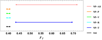
Figure 1: Fraction of transversely polarized $B_{d}^{*}$. The lines correspond to the SM, to the NP operators in Eq. (13) separately considered, and to the full set of NP operators.

The role of one operator can emerge also if other ones are taken into account. This situation is examplified in Fig. 1 that refers to the mode $B_{c}^{+}\to B_{d}^{*}\ell^{+}\nu_{\ell}$, $\ell=e,\,\mu$. [37] One can consider the fraction of $B_{d}^{*}$ that are produced with longitudinal ($F_{L}$) or transverse polarization ($F_{T}$). In the SM $F_{T}<0.5$, indicating that $B_{d}^{*}$ is produced dominantly with a longitudinal polarization. The tensor operator can reverse the hierarchy.

Contribution of the operators in (3.2.2) to various decays induced by $b\to u\ell\bar{\nu}_{\ell}$ transition.    Mode    $\epsilon_{V}$    $\epsilon_{S}$    $\epsilon_{P}$    $\epsilon_{T}$ $B^{-}\to\ell^{-}\bar{\nu}_{\ell}$ ✓ ✓ $B\to\pi\,\ell^{-}\bar{\nu}_{\ell}$ ✓ ✓ ✓ $B\to\rho\,\ell^{-}\bar{\nu}_{\ell}$ ✓ ✓ ✓ $B\to a_{1}\,\ell^{-}\bar{\nu}_{\ell}$ ✓ ✓ ✓

The role of the various operators can be inferred also considering that they contribute to a given process depending on the quantum numbers of the hadron in the final state. This is shown in Table 4.2 that refers to $b\to u\ell\nu_{\ell}$ transitions.[38] Noticeably, the couplings $\epsilon_{S}$ and $\epsilon_{P}$ are complementary to each other.

(a)

(b)

Figure 2: (a) $\Lambda_{b}\to X_{c}\tau\bar{\nu}_{\tau}$: correlation between $R_{\Lambda_{b}}(X_{c})$ and $R_{S}^{c}$. The dot corresponds to SM, the blue region to NP. (b) $\displaystyle\frac{1}{\Gamma_{b}}\frac{d\Gamma}{d\cos\theta_{P}}$ distribution in SM and in NP with different effective couplings.

In the bottom up approach a possibility to find new observables that can probe LFU is offered by semileptonic decays of beauty baryons such as $\Lambda_{b}$. In the inclusive decay $\Lambda_{b}\to X_{U}\ell\bar{\nu}_{\ell}$, defining $\theta_{P}$ as the angle between the momentum $\vec{p}_{\ell}$ of the charged lepton and the direction $\vec{s}$ of the $\Lambda_{b}$ spin, one has that $\frac{d\Gamma(\Lambda_{b}\to X_{U}\ell\bar{\nu}_{\ell})}{d{\rm cos}\theta_{P}}=A_{\ell}^{U}+B_{\ell}^{U}\,{\rm cos}\theta_{P}$. The ratio of the intercepts for $\ell=\mu$ and $\ell=\tau$ ${\cal R}_{\Lambda_{b}}(X_{U})=A_{\tau}^{U}/A_{\mu}^{U}$, analogous to ${\cal R}(D^{(*)})$, and the ratio of the slopes ${\cal R}_{S}^{U}=B_{\tau}^{U}/B_{\mu}^{U}$ represent two quantities that can probe LFU.[16] Fig. 2(a) shows that a tensor operator sizably modifies these observables with respect to the SM, while other operators have a reduced impact, as it can be inferred from the distribution in Fig. 2(b).

5 Working in the top-down approach: 331 models

Many NP models extend the SM gauge group. Among these, the 331 models[39, 40] are based on $SU(3)_{c}\otimes SU(3)_{L}\otimes U(1)_{X}$. This is first spontaneously broken to the SM group $SU(3)_{c}\otimes SU(2)_{L}\otimes U(1)_{Y}$ and then to $SU(3)_{c}\otimes U(1)_{Q}$. In such models the requirement of anomaly cancelation together with that of asymptotic freedom of QCD constrains the number of generations to be equal to the number of colours, hence answering the question of why three generations. The same request imposes that under $SU(3)_{L}$ two quark generations transform as triplets, one as an antitriplet. This is often chosen to be the third generation, and the difference possibly at the origin of the large top mass.

The electric charge operator $Q$ is related to $T_{3}$ and $T_{8}$, two of the $SU(3)$ generators, and to $X$, the generator of $U(1)_{X}$, through the relation $Q=T_{3}+\beta T_{8}+X$. $\beta$ is a parameter that defines a variant of the model.

The extension of the gauge group leads to introduce 5 new gauge bosons. Four of them are denoted by $Y^{Q_{Y}^{\pm}}$ and $V^{Q_{V}^{\pm}}$: their charges depend on the considered model variant. In all variants, a new neutral gauge boson $Z^{\prime}$ exists that mediates tree-level FCNC in the quark sector. Its couplings to leptons are instead diagonal and universal. The Higgs sector consists of three $SU(3)_{L}$ triplets and one sextet. In the fermion triplets, new heavy fermions appear together with the SM ones.

As in SM, two unitary rotation matrices $U_{L}$ (for up-type quarks) and $V_{L}$ (for down-type ones) transform flavour eigenstates into quark mass eigenstates and one has $V_{CKM}=U_{L}^{\dagger}V_{L}$. However, in SM $V_{CKM}$ appears only in charged current interactions and $U_{L},\,V_{L}$ do not appear individually. Instead, in 331 models only one matrix between $U_{L}$ and $V_{L}$ can be expressed in terms of $V_{CKM}$ and the other one. The remaining rotation matrix is usually chosen to be $V_{L}$. It enters in the $Z^{\prime}$ couplings to quarks, and it is parametrized in terms of three angles $\tilde{\theta}_{ij}$ ($i,j=1,2,3$) with sines and cosines denoted ${\tilde{c}}_{ij},\,{\tilde{s}}_{ij}$, and three phases $\delta_{i}$ ($i=1,2,3$). The Feynmann rules for $Z^{\prime}$ couplings to quarks[41], show that the $b\to d$ transition, relevant for the $B_{d}$ system, involves only the parameters ${\tilde{s}}_{13}$ and $\delta_{1}$, while the $B_{s}$ system depends on ${\tilde{s}}_{23}$ and $\delta_{2}$.[41] A peculiar feature is that also the $s\to d$ transition, relevant for the kaon sector, and the $c\to u$ one, relevant for charm processes, depend on ${\tilde{s}}_{13}$, ${\tilde{s}}_{23}$ and $\delta_{2}$, $\delta_{1}$. [42, 43] Hence, stringent correlations among flavour observables are predicted, they can discriminate this model from others. In order to derive such correlations in a given 331 variant one preliminarly finds allowed regions, oases, for the four parameters ${\tilde{s}}_{13}$, ${\tilde{s}}_{23}$, $\delta_{2}$, $\delta_{1}$ in which experimental data on selected flavour observables are reproduced within their uncertainty. These are usually chosen to be the mass differences $B_{d}-{\bar{B}}_{d}$, $B_{s}-{\bar{B}}_{s}$, $K^{0}-{\bar{K}}^{0}$; the CP asymmetries $S_{J/\psi\,K_{S}}$ in the mode $B^{0}\to J/\psi K_{S}$ and $S_{J/\psi\,\phi}$ in $B_{s}\to J/\psi\phi$; the parameter $\epsilon_{K}$ related to CP violation in the kaon system. In the SM these observables are related to the neutral meson oscillations described through box diagrams. In 331 models a new contribution is given by the tree-level diagram mediated by $Z^{\prime}$.

The SM prediction for a given flavour observable depends on the CKM parameters. Choosing $|V_{cb}|$ and $|V_{ub}|$ as two of the independent parameters of $V_{CKM}$ one can study correlations among flavour observables in selected ranges of these CKM elements. Fig. 3 shows the correlation between ${\cal B}(K^{+}\to\pi^{+}\nu\bar{\nu})$ and ${\bar{\cal B}}(B_{s}\to\mu^{+}\mu^{-})$ in one 331 variant.[44] The inclusive values of $|V_{cb}|$ correspond to points that can be compatible with the experimental result for ${\bar{\cal B}}(B_{s}\to\mu^{+}\mu^{-})$ performing slightly better than the SM corresponding to ${\cal B}(K^{+}\to\pi^{+}\nu\bar{\nu})\leq 10^{10}$. Exclusive values of $|V_{cb}|$ produce values of ${\bar{\cal B}}(B_{s}\to\mu^{+}\mu^{-})$ and ${\cal B}(K^{+}\to\pi^{+}\nu\bar{\nu})$ simultaneously smaller than the experimental range, a prediction that can be used to test this variant.

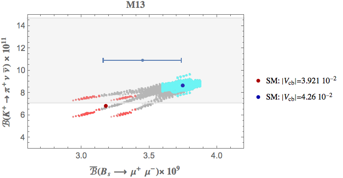
Figure 3: Correlation between ${\cal B}(K^{+}\to\pi^{+}\nu\bar{\nu})$ and ${\bar{\cal B}}(B_{s}\to\mu^{+}\mu^{-})$. The gray points span all the allowed parameter space. The red ones correspond to $|V_{cb}|\in[0.0386,\,0.0398]$, the cyan to $|V_{cb}|\in[0.0422,\,0.043]$. The SM results are shown for two values of $|V_{cb}|$ in the legenda. The light gray region and the blue range are the experimental ranges of ${\cal B}(K^{+}\to\pi^{+}\nu\bar{\nu})$ and ${\bar{\cal B}}(B_{s}\to\mu^{+}\mu^{-})$.

6 Conclusions and perspectives

Many novelties enrich the panorama of flavour physics. Among these, the flavour anomalies prompting efforts to reveal NP. Besides those discussed in this lecture, other important ones are the anomalous magnetic moment of the muon and the related problem of the hadronic $e^{+}e^{-}$ cross section; the CP violating parameter $\epsilon^{\prime}/\epsilon$ in kaon decays. Other investigations should be pursued looking for processes forbidden in the SM as lepton decays $\mu^{-}\to e^{-}\gamma$, $\mu^{-}\to e^{-}e^{+}e^{-}$. Remarkably flavour observables can access NP scales higher than direct searches foreseen in the near future [45] confirming this sector as very promising to discover BSM physics.

References

- [1] B. Grzadkowski, M. Iskrzynski, M. Misiak and J. Rosiek, Dimension-Six Terms in the Standard Model Lagrangian, JHEP 10, p. 085 (2010).
- [2] R. L. Workman et al., Review of Particle Physics, PTEP 2022, p. 083C01 (2022).
- [3] L. Wolfenstein, Parametrization of the Kobayashi-Maskawa Matrix, Phys. Rev. Lett. 51, p. 1945 (1983).
- [4] A. J. Buras, M. E. Lautenbacher and G. Ostermaier, Waiting for the top quark mass, , mixing and CP asymmetries in B decays, Phys. Rev. D 50, 3433 (1994).
- [5] M. Schmidtler and K. R. Schubert, Experimental constraints on the phase in the Cabibbo-Kobayashi-Maskawa matrix, Z. Phys. C 53, 347 (1992).
- [6] C. Jarlskog, Commutator of the quark mass matrices in the standard electroweak model and a measure of maximal nonconservation, Phys. Rev. Lett. 55, 1039 (1985).
- [7] Y. S. Amhis et al., Averages of b-hadron, c-hadron, and -lepton properties as of 2021, Phys. Rev. D 107, p. 052008 (2023).
- [8] D. Bryman, V. Cirigliano, A. Crivellin and G. Inguglia, Testing Lepton Flavor Universality with Pion, Kaon, , and Decays, Ann. Rev. Nucl. Part. Sci. 72, 69 (2022).
- [9] J. Hardy and I. Towner, Superallowed nuclear decays: 2020 critical survey, with implications for and ckm unitarity, Phys. Rev. C 102, p. 045501 (2020).
- [10] A. Crivellin, M. Kirk, T. Kitahara and F. Mescia, Global fit of modified quark couplings to EW gauge bosons and vector-like quarks in light of the Cabibbo angle anomaly, JHEP 03, p. 234 (2023).
- [11] M. Neubert, Heavy quark symmetry, Phys. Rept. 245, 259 (1994).
- [12] M. E. Luke, Effects of subleading operators in the heavy quark effective theory, Phys. Lett. B 252, 447 (1990).
- [13] J. Chay, H. Georgi and B. Grinstein, Lepton energy distributions in heavy meson decays from QCD, Phys. Lett. B 247, 399 (1990).
- [14] I. I. Bigi, M. A. Shifman, N. Uraltsev and A. I. Vainshtein, QCD predictions for lepton spectra in inclusive heavy flavor decays, Phys. Rev. Lett. 71, 496 (1993).
- [15] B. M. Dassinger, T. Mannel and S. Turczyk, Inclusive semi-leptonic B decays to order 1 / m(b)**4, JHEP 03, p. 087 (2007).
- [16] P. Colangelo, F. De Fazio and F. Loparco, Inclusive semileptonic decays in the Standard Model and beyond, JHEP 11, 032 (2020), [Erratum: JHEP 12, 098 (2022)].
- [17] P. Colangelo and F. De Fazio, Tension in the inclusive versus exclusive determinations of : a possible role of new physics, Phys. Rev. D 95, p. 011701 (2017).
- [18] I. Caprini, L. Lellouch and M. Neubert, Dispersive bounds on the shape of lepton anti-neutrino form-factors, Nucl. Phys. B530, 153 (1998).
- [19] A. Abdesselam et al., Measurement of the branching ratio of relative to decays with a semileptonic tagging method, in 51st Rencontres de Moriond on EW Interactions and Unified Theories, 3 2016.
- [20] C. G. Boyd, B. Grinstein and R. F. Lebed, Model independent extraction of using dispersion relations, Phys. Lett. B353, 306 (1995).
- [21] C. G. Boyd, B. Grinstein and R. F. Lebed, Model independent determinations of , form-factors, Nucl. Phys. B461, 493 (1996).
- [22] D. Bigi, P. Gambino and S. Schacht, A fresh look at the determination of from , Phys. Lett. B769, 441 (2017).
- [23] B. Grinstein and A. Kobach, Model-Independent Extraction of from , Phys. Lett. B771, 359 (2017).
- [24] J. P. Lees et al., Extraction of form Factors from a Four-Dimensional Angular Analysis of , Phys. Rev. Lett. 123, p. 091801 (2019).
- [25] G. Martinelli, S. Simula and L. Vittorio, Updates on the determination of , and (10 2023).
- [26] M. T. Prim et al., Measurement of differential distributions of B→D*¯ and implications on —Vcb—, Phys. Rev. D 108, p. 012002 (2023).
- [27] A. Buras, Gauge Theory of Weak Decays (Cambridge University Press, 6 2020).
- [28] A. Mathad, Recent highlights from the LHCb experiment, in 25th DAE-BRNS High Energy Physics Symposium, 8 2023.
- [29] R. Aaij et al., Measurement of -Averaged Observables in the Decay, Phys. Rev. Lett. 125, p. 011802 (2020).
- [30] R. Aaij et al., Analysis of Neutral B-Meson Decays into Two Muons, Phys. Rev. Lett. 128, p. 041801 (2022).
- [31] C. Bobeth, M. Gorbahn, T. Hermann, M. Misiak, E. Stamou and M. Steinhauser, in the Standard Model with Reduced Theoretical Uncertainty, Phys. Rev. Lett. 112, p. 101801 (2014).
- [32] S. Glazov, Belle II physics highlights, in EPS-HEP2023 Conference, Hamburg , 20-25 August 2023, https://indico.desy.de/event/34916/,
- [33] J. P. Lees et al., Evidence for an excess of decays, Phys. Rev. Lett. 109, p. 101802 (2012).
- [34] R. Aaij et al., Measurement of the ratio of branching fractions /, Phys. Rev. Lett. 120, p. 121801 (2018).
- [35] P. Biancofiore, P. Colangelo and F. De Fazio, On the anomalous enhancement observed in decays, Phys. Rev. D 87, p. 074010 (2013).
- [36] P. Colangelo and F. De Fazio, Scrutinizing and in search of new physics footprints, JHEP 06, p. 082 (2018).
- [37] P. Colangelo, F. De Fazio and F. Loparco, Role of in the Standard Model and in the search for BSM signals, Phys. Rev. D 103, p. 075019 (2021).
- [38] P. Colangelo, F. De Fazio and F. Loparco, Probing New Physics with and , Phys. Rev. D 100, p. 075037 (2019).
- [39] F. Pisano and V. Pleitez, An SU(3) x U(1) model for electroweak interactions, Phys. Rev. D 46, p. 410 (1992).
- [40] P. H. Frampton, Chiral dilepton model and the flavor question, Phys. Rev. Lett. 69, 2889 (1992).
- [41] A. J. Buras, F. De Fazio, J. Girrbach and M. Carlucci, The Anatomy of Quark Flavour Observables in 331 Models in the Flavour Precision Era, JHEP 02, p. 023 (2013).
- [42] P. Colangelo, F. De Fazio and F. Loparco, c→u¯ transitions of Bc mesons: 331 model facing Standard Model null tests, Phys. Rev. D 104, p. 115024 (2021).
- [43] A. J. Buras, P. Colangelo, F. De Fazio and F. Loparco, The charm of 331, JHEP 10, p. 021 (2021).
- [44] A. J. Buras and F. De Fazio, 331 model predictions for rare B and K decays, and F = 2 processes: an update, JHEP 03, p. 219 (2023).
- [45] R. K. Ellis et al., Physics Briefing Book: Input for the European Strategy for Particle Physics Update 2020.