Black hole models II: Kerr–Vaidya solutions

Abstract

In the second part of a three-fold series, we examine semi-classical models of black holes and white holes, generalizing to the axisymmetric case by modelling their near-horizon geometry via the radiative Kerr-Vaidya metrics. We examine the form of the energy-momentum tensor (EMT) near the apparent horizon and the experiences of various observers. Two out of the four possible classes of Kerr–Vaidya solutions are counterparts of their spherically-symmetric self-consistent solutions: evaporating black holes and expanding white holes. We demonstrate a consistent description of an accreting black hole based on the ingoing Kerr-Vaidya metric with increasing mass, and further show that the model can be extended to the case where the angular momentum to mass ratio varies. However, pathologies are identified in the expanding white hole geometry which reinforce controversies arising from the classical and quantum instabilities of their static counterparts. We also show that the apparent horizon of a Kerr-Vaidya black hole admits a description in terms of a Rindler horizon.

I Introduction

Astrophysical black holes (ABHs) are dark, massive objects compact enough to possess a light ring, and are believed to number in the hundreds of millions in the Milky Way alone. Models that attempt to describe ABHs typically fall into one of two distinct groups: those with and those without horizons. The latter category includes a variety of proposals, including gravitational condensates (gravastars), fuzzballs, and 2-2 holes, while the former is based on the stationary Schwarzschild and Kerr solutions of classical general relativity [1, 2]. Their defining features are the event horizon, a null surface that causally disconnects the black hole interior from the outside world, and the singularity, where curvature scalars diverge and the validity of general relativity breaks down. Solutions with an event horizon and singularity are referred as mathematical black holes (MBHs). They have long been used as de facto proxies for studying black holes in both astrophysical and purely theoretical settings [3, 4, 6, 7, 5, 8, 9]. Despite this, the notion that ABHs can identified with MBHs remains a speculation rather than an observationally established fact [2].

For ordinary classical matter, MBHs describe the asymptotic result of gravitational collapse [3, 6]. In practice they provide an excellent description of all current ABH observations [1] despite only representing asymptotic states, since the blackening of a collapsar happens exponentially fast from the point of view of a distant observer Bob. Likewise, the crossing of the event horizon of a MBH happens in finite time according to an infalling observer Alice. These two results motivate (usually implicitly) the treatment of certain MBH features — such as the horizon — as being real entities that need to be accounted for in a physical description of ABHs.

However, the identification of MBHs with ABHs is both technically and conceptually problematic. While MBHs exteriors are regular, their interiors contain Cauchy horizons and singularities. At the same time, the event horizon represents a teleological entity whose global nature renders it inaccessible to local observers. Its existence generates a host of technical difficulties as well as the celebrated information loss problem [6, 10, 11, 12]. To make matters more complicated, quantum effects such as Hawking radiation violate all classical energy conditions [3, 13] thereby invalidating traditional arguments against the finite formation time observed by Bob. These issues have motivated the development of horizonless models of ABHs, which come with their own share of conceptual difficulties [1, 14].

Our goal is to investigate the consequences of horizon formation as perceived by distant observers. Hence, we do not commit to the formation of a fully-fledged MBH, instead focussing on the most important feature of a black hole — the trapping of light. The apparent horizon is the boundary of the trapped region, and the trapped region itself is identified as the physical black hole (PBH). The occurrence of other features such as a singularity is not assumed. Our essential requirements are then the following: crossing into the trapped region (or signalling from its boundary) occurs in finite time according to a distant observer Bob, and the boundary of the trapped region is singularity-free in the weakest possible sense. The latter is accomplished by requiring that polynomial invariants built from components of the Riemann curvature tensor are finite [14].

Note that the preceding discussion, and a large fraction of the conceptual discussions surrounding black holes, are formulated in semiclassical language. A complete resolution of issues formulated in the semiclassical framework is provided (up to the scale where full quantum gravitational effects are expected [10]) by simultaneously solving the semiclassical Einstein equations and the propagation of quantum fields on the resulting background. Unfortunately, no fully tractable method for solving the semiclassical Einstein equations in a general setting is known. Instead, we take as a starting point some of the expected features of the solutions and incorporate them into a self-consistent semiclassical framework, which can be used both to exclude existing models on the basis of observationally motivated criteria, and to construct new models consistent with our expected operational experiences [14].

In spherical symmetry the requirements of finite time of horizon formation (as seen by a distant observer Bob) and weak regularity lead to a complete characterization of the near-horizon geometry of a PBH, along with a distinguished class of PBH formation scenarios. One of the consequences of finite formation time is a generic violation of the null energy condition (NEC) [3, 6, 7] near the outer apparent horizon (anti-trapping horizon), and a constraint on the dynamical evolution of the associated solutions: physical black holes must evaporate and their white hole counterparts must grow [15, 16, 14].

However, ABHs are not expected to be spherically symmetric. While their angular momentum is significantly more difficult to measure relative to their mass (which is determined by their far-field influence), most ABH populations are now known to dominated by spinning objects. X-ray reflection measurements indicate that the majority of supermassive black holes and X-ray binaries are rapidly spinning ($a=J/M>0.9$) [17, 18], while more tentative gravitational wave measurements of binary mergers reveal populations of slowly rotating stellar-mass black holes [19]. At the technical level however, moving to axial symmetry introduces a number of challenges due to the reduced symmetry and non-static nature of the implied metric [3, 4], but also to a host of important effects not present in the spherical case. As a result, generalizing black hole models to the axisymmetric case is of primary interest.

The first paper in this series [20] examined the modelling of ABHs in a spherically symmetric setting. In this second paper, we analyze the simplest dynamical axially symmetric case. We focus on the ‘radiative’ Kerr–Vaidya metric and identify four distinct Kerr–Vaidya solutions, two representing black holes and two representing white holes, with all four solutions violating the null energy condition (NEC). This property makes the Kerr–Vaidya metrics suitable for modelling the near-horizon geometry of physical black holes, where NEC violation is required for the apparent horizon to be visible by distant observers [3, 6] and for Hawking evaporation to occur.

As a preamble, we describe properties of the spherically-symmetric white hole solutions. We also analyse Vaidya metrics in advanced coordinates with decreasing mass, which correspond to contracting white holes and are ruled out by our basic assumptions. While known that it is possible to reach scalar curvature singularities by ingoing radial null geodesics [21], we show how families of timelike geodesics starting from outside the event horizon can reach this singularity at the moment of final evaporation. This timelike geodesic incompleteness is also present in the Kerr–Vaidya counterparts of these metrics, providing additional arguments against the physical relevance of white hole solutions.

We also consider scenarios where the angular momentum to mass ratio varies as a function of time. While the Kerr–Vaidya metric with variable $a=J/M$ presents some difficulties (such as having no Kerr-Schild form ) it is nonetheless necessary in view of both Hawking radiation, through which particle emission can shed angular momentum faster than mass [22, 23, 24], and in astrophysical settings, where interaction with the accretion disk can remove angular momentum with enormous efficiency through variants of the Penrose process [25]. We examine the asymptotic behaviour of the Kerr–Vaidya metric with variable $a$, and show that contrary to some earlier indications, asymptotic flatness can be maintained.

Finally we discuss the equivalence (in the near-horizon approximation) of the Rindler and Schwarzschild horizons in the axially symmetric case. In both the constant and variable angular momentum to mass ratios we demonstrate that two different notions of horizon— of the Rindler horizon and the separatrix— are equivalent in the near-horizon approximation.

The rest of this paper is organized as follows. In Sec. II we review the relevant properties of the spherically symmetric solutions. In Sec. III we discuss their axially symmetric counterparts, focusing on the violation of the energy conditions, the location of the apparent horizons, and the presence of a firewall. In Sec. IV, we present some features of Kerr–Vaidya spacetimes whose angular momentum per unit mass are functions of ingoing/outgoing coordinates. We conclude in Sec VI with a summary of our results, their implications, and directions for future work. Throughout, we work in units where $\hbar=c=G=1$ and use the $(-+++)$ signature.

II Spherically symmetric solutions

We provide a brief summary of the self-consistent approach and some key features of physical black holes in Sec. II.1. Additional details can be found in Refs. [14, 20]. Sec. II.2 presents the key properties of the white hole solutions.

II.1 The self-consistent approach and its black hole solutions

Semiclassical gravity describes the effects of quantized matter fields on classical spacetime geometry, which itself is described by a metric $\textsl{g}_{\mu\nu}$. The classical notions of test particles’ trajectories, horizons, etc. are assumed to be well-defined. The metric itself is a solution of the Einstein equations, which may include higher-order curvature terms and a cosmological constant,

$$R_{\mu\nu}-{\tfrac{1}{2}}\textsl{g}_{\mu\nu}R=8\pi T_{\mu\nu}\ ,$$ (1)

where $R_{\mu\nu}$ and $R$ are the Ricci tensor and scalar, respectively. Their source is the expectation value of the renormalized energy-momentum tensor $T_{\mu\nu}\vcentcolon={\langle}\hat{T}_{\mu\nu}{\rangle}_{\omega}$, and it includes some or all of the contributions described above.

A full semiclassical scheme is in principle completed by an evolution equation for the state $\omega$ on the background $\textsl{g}_{\mu\nu}$ [10]. Our self-consistent approach [14] is based solely on existence of such a state, the formation of the relevant horizon in a finite time according to a distant observer, and minimal regularity requirements.

A general spherically symmetric metric in Schwarzschild coordinates [4, 9] is given by

$$ds^{2}=-e^{2h(t,r)}f(t,r)dt^{2}+f(t,r)^{-1}dr^{2}+r^{2}d\Omega_{2}\ .$$ (2)

In terms of the advanced null coordinate $v$ the metric is

$$ds^{2}=-e^{2h_{+}(v,r)}f_{+}(v,r)dv^{2}+2e^{h_{+}(v,r)}dvdr+r^{2}d\Omega_{2}\ ,$$ (3)

and using the retarded null coordinate $u$ it is written as

$$ds^{2}=-e^{2h_{-}(u,r)}f_{-}(u,r)dv^{2}-2e^{h_{-}(u,r)}dudr+r^{2}d\Omega_{2}\ .$$ (4)

The function $f$ is coordinate-independent, i.e. $f(t,r)\equiv f_{+}\big{(}v(t,r),r\big{)}$ and in what follows we omit the subscript. It is conveniently represented via the Misner–Sharp–Hernandez (MSH) mass $M\equiv C/2$ as

$${\partial}_{\mu}r{\partial}^{\mu}r\equiv f=\vcentcolon 1-\frac{C(t,r)}{r}=1-\frac{C_{+}(v,r)}{r}\ ,$$ (5)

where the coordinate $r$ is the areal radius [9]. The functions $h$ and $h_{\pm}$ play the role of integrating factors in coordinate transformations, such as Eq. (19) below.

Analysis of the Einstein equations and the evaluation of curvature invariants are conveniently performed using the effective EMT components $\tau_{a}$, (where $a={}_{t},{}^{r},{}_{t}{}^{r}$) [14]

$$\tau{{}_{t}}\vcentcolon=e^{-2h}{T}_{tt}\ ,\qquad{\tau}{{}^{r}}\vcentcolon=T^{rr}\ ,\qquad\tau{{}_{t}^{r}}\vcentcolon=e^{-h}{T}{{}_{t}^{r}}\ .$$ (6)

The Einstein equations for the components $G_{tt}$, ${G_{t}}^{r}$, and ${G}^{rr}$ are then, respectively

$$\partial_{r}C =8\pi r^{2}{\tau}{{}_{t}}/f\ ,$$ (7)

$$\partial_{t}C =8\pi r^{2}e^{h}{\tau_{t}}^{r}\ ,$$ (8)

$$\partial_{r}h =4\pi r\left({\tau}{{}_{t}}+{\tau}{{}^{r}}\right)/f^{2}\ .$$ (9)

A PBH is a trapped region — a domain where both ingoing and outgoing future-directed null geodesics emanating from a spacelike two-dimensional surface with spherical topology have negative expansion [3, 9]. The apparent horizon is the boundary of this trapped region that corresponds to the domain $f<0$ in Eq. (3). In an asymptotically flat spacetime the Schwarzschild radius $r_{\textsl{g}}$ is the largest root of $f(t,r)=0$ (see Ref. [14] and the references therein for the detailed summary of the definitions and their consequences). Invariance of the MSH mass implies that

$$r_{\textsl{g}}(t)=C(t,r_{\textsl{g}})=r_{+}\big{(}v(t,r_{\textsl{g}}(t))\big{)}\ ,$$ (10)

where $r_{+}(v)$ is the largest root of $f_{+}(v,r)=0$. It represents the location of the outer component of the apparent horizon of a black hole or the anti-trapping horizon of a white hole. Unlike the globally defined event horizon, the notion of the apparent horizon is foliation-dependent. However, it is invariantly defined in all foliations that respect spherical symmetry [26].

Our regularity requirement is the weakest form of the cosmic censorship conjecture [6, 9]: all polynomial invariants that are based on the contractions of the Riemann tensor [3, 7] are finite up to and on the apparent horizon. Constructing finite invariants from the divergent quantities that describe a real-valued solution allows one to describe properties of the near-horizon geometry. It is sufficient to ensure that only two of them, $R$ and $R_{\mu\nu}R^{\mu\nu}$, are finite [27]. Moreover, we focus on the quantities,

$$\mathrm{T}\vcentcolon=({\tau}{{}^{r}}-{\tau}{{}_{t}})/f,$$ (11)

$$\mathfrak{T}\vcentcolon=\big{(}({\tau}{{}^{r}})^{2}+({\tau}{{}_{t}})^{2}-2({\tau}{{}_{t}^{r}})^{2}\big{)}/f^{2}\ ,$$ (12)

which are only parts of the full expressions for the curvature scalars

$$T^{\mu}_{~{}\nu}=\mathrm{T}+2T^{\theta}_{~{}\theta},\qquad T^{\mu\nu}T_{\mu\nu}=\mathfrak{T}+2\big{(}T^{\theta}_{~{}\theta}\big{)}^{2}.$$ (13)

The contributions from $T^{\theta}_{~{}\theta}\equiv T^{\phi}_{~{}\phi}$ can initially be disregarded, as one can verify that they do not introduce further divergences [14, 27]. Because the metric in Schwarzschild coordinates is singular at the apparent horizon, working instead with $(u,r)$ and $(v,r)$ coordinates allows one to identify the resulting solutions. Note that in $1+1$ dimensions the condition of regularity at the horizon is known to be equivalent to its formation in finite time, however it is not known whether this is the case in $3+1$ dimensions [28].

The assumptions of finite formation time and regularity restrict the scaling of the effective EMT components near the Schwarzschild radius, such that $\tau_{a}\propto f^{k}$, with $k=0,1$. Solutions with $k=0$ describe a PBH after formation (and before a possible disappearance of the trapped region). Vaidya metrics, and dynamical regular black hole solutions belong to this class [29], while the Reissner-Nordström solution or static RBH solutions correspond to $k=1$. In the following we work with $k=0$ solutions.

The EMT components of the $k=0$ solutions satisfy

$$\lim_{r\to r_{\textsl{g}}}\tau_{t}=\lim_{r\to r_{\textsl{g}}}\tau^{r}=-\Upsilon^{2}(t)\ ,\quad\lim_{r\to r_{\textsl{g}}}\tau^{r}_{t}=\pm\Upsilon^{2}(t)\ ,$$ (14)

for some function $\Upsilon(t)>0$. The leading terms of the metric functions in a near-horizon expansion are given in terms of $x\vcentcolon=r-r_{\textsl{g}}(t)$ as

$$C =r_{\textsl{g}}-4\sqrt{\pi}r_{\textsl{g}}^{3/2}\Upsilon\sqrt{x}+\mathcal{O}(x)\ ,$$ (15)

$$h =-\frac{1}{2}\ln{\frac{x}{\xi}}+\mathcal{O}(\sqrt{x})\ .$$ (16)

The function $\Upsilon(t)$ determines the energy density, pressure and flux at the apparent horizon, and $\xi(t)$ is determined by choice of the time variable.

The Einstein equation (8) serves as a consistency condition and establishes the relation between the rate of change of the MSH mass and the leading terms of the metric functions,

$$r^{\prime}_{\textsl{g}}/\sqrt{\xi}=\pm 4\sqrt{\pi r_{\textsl{g}}}\,\Upsilon\ .$$ (17)

The EMT near the Schwarzschild sphere is

$$\ T^{a}_{~{}b}=\begin{pmatrix}\Upsilon^{2}/f&\pm e^{-h}\Upsilon^{2}/f^{2}\vspace{1mm}&0&0\\ \mp e^{h}\Upsilon^{2}&-\Upsilon^{2}/f&0&0\\ 0&0&p_{\|}&0\\ 0&0&0&p_{\|}\end{pmatrix}\ ,$$ (18)

where the upper sign corresponds to the (evaporating) PBH and the tangential pressure $p_{\|}$ is finite at $r=r_{\textsl{g}}$. Both signs lead to the violation of the NEC. In particular this means that out of the four possible types of Vaidya metrics, $h_{\pm}=0$, $f=1-r_{+}(v)/r$, or $f=1-r_{-}(u)/r$, only the solutions with $r_{+}^{\prime}<0$ and $r_{-}^{\prime}>0$ are allowed [14]. The retreating apparent horizon and the advancing anti-trapping horizon are timelike surfaces [30].

Consider the energy density $\varrho=T_{\mu\nu}u^{\mu}u^{\nu}$, the pressure $p=T_{\mu\nu}n^{\mu}n^{\nu}=T^{r}_{~{}r}$, and the flux $\varphi=T_{\mu\nu}u^{\mu}n^{\nu}$ that are perceived by various observers with four-velocities $u^{\mu}$ and outward-pointing radial spacelike vector $n^{\mu}$. For an observer at constant $r$ all of these quantities, $\varrho=-T^{t}_{~{}t}$, $p=T^{r}_{~{}r}$, diverge in the limit $r\to r_{\textsl{g}}$. The experience of an infalling observer Alice is different for a PBH compared to a white hole.

A radially infalling (geodesic) observer Alice moves along a trajectory given by $x^{\mu}_{\mathrm{A}}(\tau)$. Horizon crossing happens not only at some finite proper time $\tau_{0}$, where $r_{\textsl{g}}\big{(}t(\tau_{0})\big{)}=r(\tau_{0})$, but due to the form of the metric also at a finite time $t(\tau_{0})$ according to a distant observer Bob. Moreover, the energy density, pressure and flux in Alice’s frame are finite [27, 14].

II.2 White hole solutions

A white hole is an anti-trapped region — a domain where both ingoing and outgoing future-directed null geodesics emanating from a spacelike two-dimensional surface with spherical topology have positive expansion. The anti-trapping horizon is the boundary of this trapped region.

II.2.1 Physical white holes

White hole solutions in the self-consistent approach correspond to $r_{\textsl{g}}^{\prime}>0$ and are conveniently described using $(u,r)$ coordinates [30, 15]. The retarded null coordinate $u$,

$$dt=e^{-h}(e^{h_{-}}du+f^{-1}dr)\ ,$$ (19)

is regular across the expanding anti-trapping horizon. In analogy with PBHs, we refer to white holes that form in finite time according to Bob as physical white holes (PWHs). The name, however, does not imply that these objects are necessarily found in nature.

Using the Einstein equations and the relationships between components of the EMT in two coordinates systems one can show that

$$C_{-}(u,r)=r_{-}(u)+w_{1}(u)y+\ldots\ ,$$ (20)

$$h_{-}(u,r)=\chi_{1}(u)y+\ldots\ ,$$ (21)

where $r_{-}(u)$ is the radial coordinate of the apparent horizon, we define $y\vcentcolon=r-r_{-}(u)$, and $C_{-}(u,r_{-})\equiv r_{-}$. The Vaidya geometry with $C^{\prime}_{-}(u)=2M^{\prime}(u)>0$ and $h_{-}\equiv 0$ is the simplest example of such a white hole. Some relationships with the quantities in $(t,r)$ coordinates are summarized in Appendix A.1, and more details are given in Ref. [14].

(a)

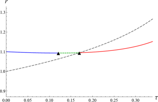
(b)

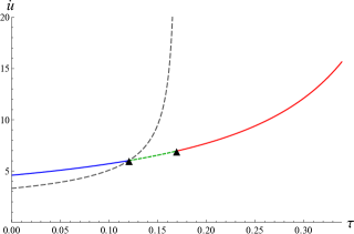
Figure 1: Entry of a massive test particle into the Vaidya white hole. Both figures are based on the linear accretion law $r_{-}(u)=r_{-}(0)-\alpha u$ with $r_{-}(0)=1$ and $\alpha=0.1$ The initial conditions are $u(0)=0$, $r(0)=1.1$ and $\dot{r}(0)=-0.1$. (a) Trajectory from the initial moment until the reversal and the capture. The areal radius $r(\tau)$ and the (outer) apparent horizon $r_{+}\big{(}v(\tau)\big{)}$ (gray dashed line) are shown as functions of the proper time $\tau$. (b) Segments of the trajectory showing the “reversal” (the geodesic switches from being outgoing to ingoing) and capture. The time derivative $\dot{u}$ is shown as a solid line, and the limiting value $\sqrt{f\big{(}u(\tau),r(\tau)\big{)}}$ as a dashed gray line.

The anti-trapped region of a classical (“eternal”) white hole is inaccessible to external observers. However, as the anti-trapping horizon of a PWH at $r_{\textsl{g}}\equiv r_{-}$ is timelike [30], test particles can cross it. To focus on the essential features we describe the near-horizon geometry by a Vaidya metric in retarded coordinates. Null geodesics on the Vaidya background can be reduced to a system of first-order equations, and for the linear case $C_{-}(u)=r_{0}+\alpha u$ an adaptation of the methods in [49] leads to an analytic solution (see Appendix A.2 for details).

The motion of timelike test particles is more intricate. Outside of the anti-trapped region, both ingoing and outgoing radial trajectories with four-velocity $u_{\mathrm{A}}=(\dot{u},\dot{r},0,0)$ satisfy the relation

$$\dot{u}=\frac{-\dot{r}+\sqrt{\dot{r}^{2}+f}}{f}\ ,$$ (22)

where $f=1-r_{-}\big{(}u(\tau)\big{)}/r(\tau)$. This follows from the timelike condition $u_{\mathrm{A}}^{\mu}u_{\mathrm{A}\,\mu}=-1$ and the future-directedness of the coordinate $u$, namely $\dot{u}>0$. The geodesic equations for radial timelike geodesics are

$$\ddot{r}=-\frac{r_{-}}{2r^{2}}+\frac{r^{\prime}_{-}}{2r}\dot{u}^{2}\ ,$$ (23)

$$\ddot{u}=\frac{r_{-}}{2r^{2}}\dot{u}^{2}\ ,$$ (24)

where the first term on the right-hand side of Eq. (23) is absent for null geodesics.

Inside the region $f<0$ the areal radius can only grow and thus the radial velocity component is positive ($\dot{r}>0$) which is consistent with having $\ddot{r}>0$ near $r_{-}$. As a result, there are two a priori possible entry scenarios: either $\dot{r}(\tau)$ becomes zero upon entry at $r(\tau)=r_{-}\big{(}u(\tau)\big{)}$, or at some $r=r_{*}>r_{-}$ the infall stops, the particle becomes outgoing, and is then overtaken by the expanding horizon. We will now show that only the latter option is possible. Assume, to the contrary, that the radial velocity goes to zero at the horizon crossing. Then

$$\lim_{r(\tau)\to r_{-}(u(\tau))}\frac{\dot{r}^{2}}{f}=A\ ,$$ (25)

where $A$ depends on the initial conditions and a priori can be either finite or infinite. In both cases $\dot{u}$ and $\ddot{u}$ diverge. However, the divergences obtained from $\ddot{u}$ as determined by the geodesic equation (24), and as calculated directly from the proper time derivative of $\dot{u}$, are not consistent with each other. For example, if $A=0$, then according to Eq. (24) $\ddot{u}$ should diverge as $f^{-1}$, while Eq. (22) implies an $f^{-2}$ divergence. Hence the radial velocity cannot go to zero at the horizon, and the only valid entry scenario involves the particle turning around and being overtaken by the expanding horizon.

We illustrate this using a simple model of a linearly expanding Vaidya PWH. Fig. 1 shows the trajectory of a massive, initially ingoing test particle. Eq. (22) implies that for ingoing particles $\dot{u}\geqslant 1/\sqrt{f}$. This value is reached when $\dot{r}=0$, at which point the particle reverses direction and starts moving radially outward, where it may be overtaken by the expanding apparent horizon. The associated energy density, flux and pressure in the proper frame of the test particle when it enters the white hole are finite (see Appendix A.1),

$$\varrho_{\mathrm{A}}=-\varphi_{\mathrm{A}}=p_{\mathrm{A}}=-\frac{r^{\prime}_{-}(u)}{8\pi r^{2}\dot{r}^{2}}\ .$$ (26)

White hole and black hole solutions can be conveniently described as time reverses of each other. For Vaidya metrics this is accomplished by taking $v\to-u$. The complicated entry scenario described above has a counterpart in the exit of test particles from an evaporating Vaidya black hole. There, outgoing geodesics are reversed and become ingoing, and subsequently may be overtaken by the contracting apparent horizon [31].

However, some of the usual interpretations of the role of the Vaidya metric in modelling evaporating black holes with $r^{\prime}(v)<0$ and do not directly translate to the white holes with $r^{\prime}(u)>0$ . In both cases the event horizon is hidden by the apparent/anti-trapping horizon, but in the black hole case the ingoing Vaidya metric with $r^{\prime}(v)<0$ is consistent with the requirement that one has a future horizon and a decreasing mass due to Hawking evaporation. Such an approximation is usually taken to be valid near the horizon ($r\lesssim r_{\textsl{g}}$) where the NEC violation is interpreted as a flux of negative energy (as defined by a timelike Killing vector in the asymptotic region) across the horizon, which serves to reduce the black hole mass [11, 6].

The corresponding white hole geometry contains a near-horizon region described by an outgoing Vaidya metric with $r_{-}^{\prime}(u)>0$, as the evaporating case does not correspond to the finite formation time according to distant Bob. However, the physical interpretation of the NEC violating null fluid in the black hole case does not readily carry over to the white hole geometry. Since $r^{\prime}(u)>0$, the outgoing flux must be of negative energy modes in order for the mass to increase. However, contrary to the black hole case where such modes tunnel from a classically forbidden region (outside the horizon) to one where their momenta are timelike (inside the horizon) [6, 11, 12], the modes here would be of negative energy outside the horizon.

As a result, the interpretation of Hawking radiation as a tunnelling process across the horizon is incompatible with the consistency conditions we impose, when applied to the semiclassical white hole geometry. This is not entirely surprising given the numerous pathologies that arise when describing the Hawking process in a white hole background. In the (eternal) black hole background, the late-time thermal density matrix constituting Hawking radiation is insensitive to ambiguities in defining a notion of positive frequency for horizon states. For the white hole geometry the state of the field observed at future null infinity $\mathcal{I}^{+}$ is quite arbitrary, depending strongly on the choice of state in the asymptotic past $\mathcal{I}^{-}$ and on the past horizon $\mathcal{H}_{-}$. A simple time-reversal of the Unruh state defined in the evaporating black hole case produces a state with an unnaturally high degree of correlation between $\mathcal{I}^{-}$ and $\mathcal{H}_{-}$ and no flux at $\mathcal{I}^{+}$, while more natural choices produce divergent outgoing fluxes which invalidate the semiclassical approximation [32].

II.2.2 Evaporating Vaidya white holes

The anti-trapping horizon of an evaporating spherically symmetric white hole is inaccessible to distant observers, as the NEC is satisfied [3]. As Vaidya metrics capture the essential features of the near horizon geometry of these solutions, we focus on the metric

$$ds^{2}=-\left(1-\frac{r_{-}(u)}{r}\right)du^{2}-2dudr+r^{2}d\Omega_{2}\ ,$$ (27)

with $r_{-}^{\prime}<0$. Fig. 2 depicts several scenarios where $r_{-}(u)=2M(u)$ goes to zero at $u=0$. The details of the joining with the Minkowskian domain depend not only on the value of

$$\alpha_{0}=-r^{\prime}_{-}(0)=-\lim_{u\to 0}r_{-}/u\ ,$$ (28)

but also on the intermediate history [21], while the early history at $u\to-\infty$ determines the structure of the diagrams near past timelike and null infinity.

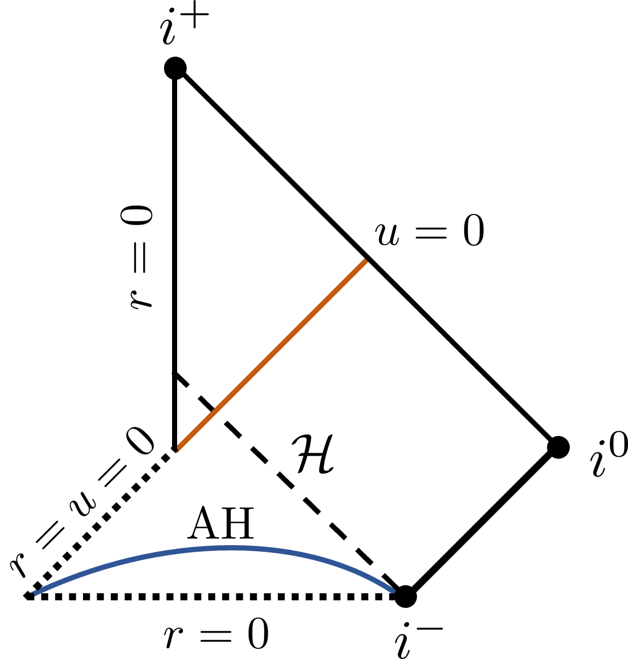
(a)

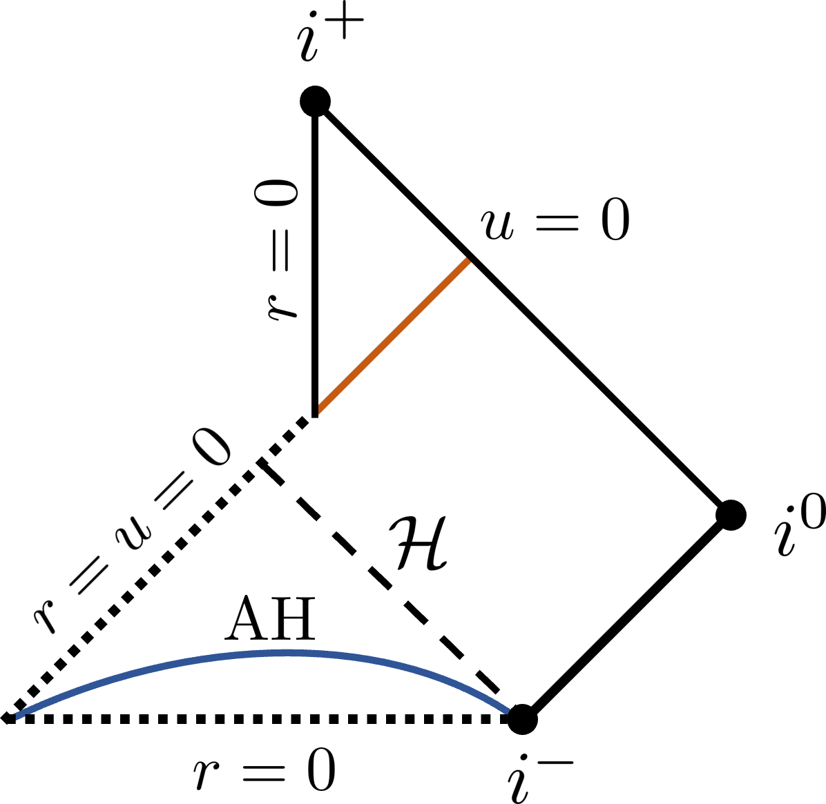
(b)

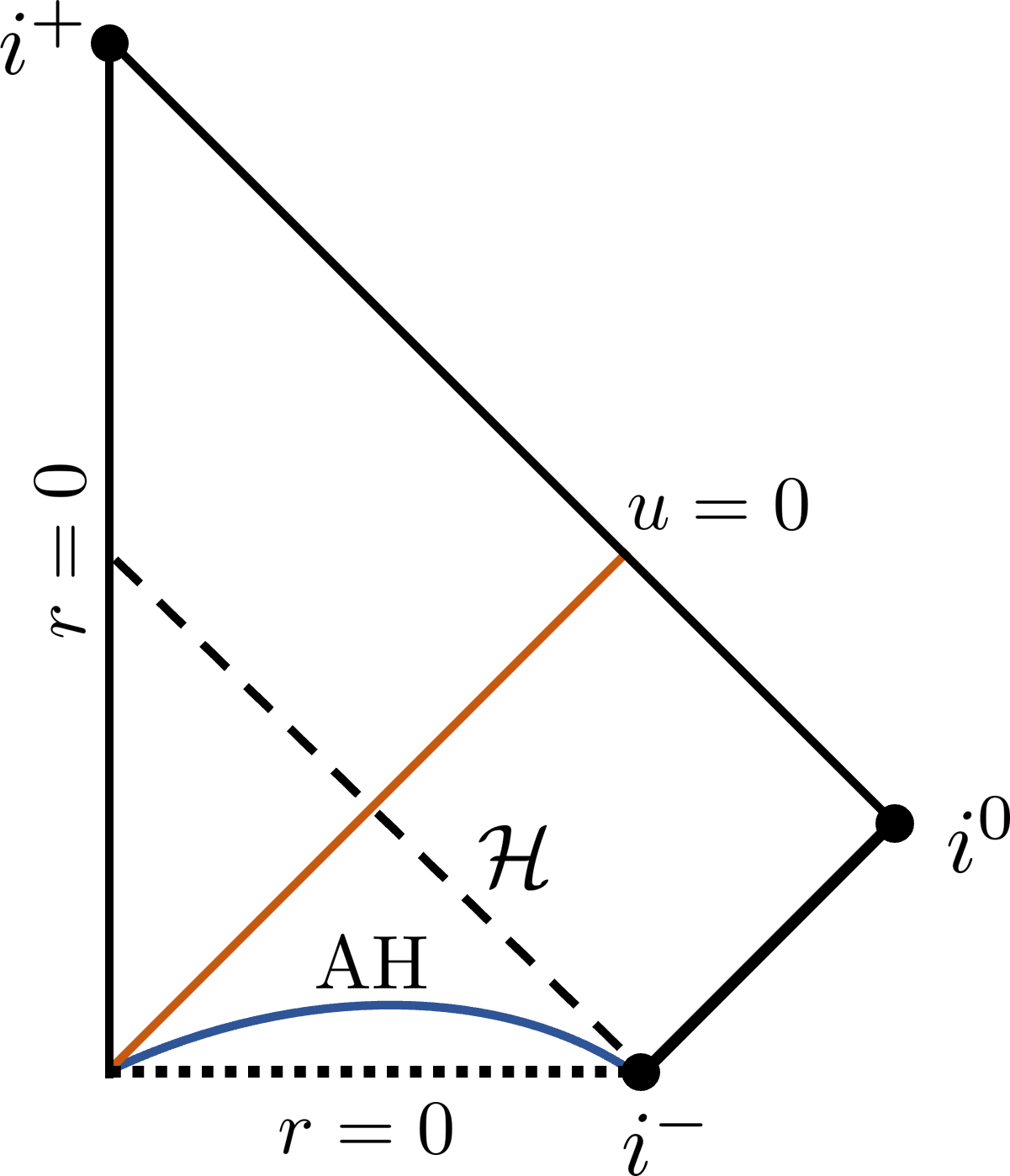
(c)

Figure 2: Some possible Carter–Penrose diagrams of evaporating white holes, with complete evaporation occurring at $u=0$. Curvature singularities are shown as a dotted lines. The null singularity at $r=u=0$ may (a) or may not (b) lie inside the past horizon $\mathcal{H}$ (dashed line). Blue solid AH represents the anti-trapping horizon. The Vaidya metric describes the geometry to the causal past of $u=0$, while the geometry is Minkowski afterwards. Linear evaporation $r=-\alpha u$ at the last stages of the evolution correspond to the diagrams (b) $0<\alpha<1/8$, and (c) $\alpha>1/8$.

Analysis of the causal structure, including the extensions of Vaidya spacetimes, is naturally performed using null geodesics. However, studies of timelike geodesics are also important and may reveal crucial features of the spacetime [3, 7].

For timelike trajectories in the vicinity of the horizon it is convenient to monitor the gap function [33]

$$z(\tau)\vcentcolon=r(\tau)-r_{-}\big{(}u(\tau)\big{)}\ .$$ (29)

For ingoing observers its proper rate of change is

$$\dot{z}=\dot{r}-r^{\prime}\dot{u}=-|\dot{r}|\left(1-\frac{2}{z}|r_{-}^{\prime}|r_{-}\right)+\mathcal{O}\big{(}z^{0}\big{)}\ ,$$ (30)

where in the vicinity of the horizon we used Eq. (112). A useful fictitious surface — the gap separatrix — is introduced as the radial coordinate $r_{*}(\tau)$ such that for the given values of $u(\tau)$ and $\dot{r}(\tau)$ the value of $\dot{u}$ (that is determined via Eq. (22) as a function of $u$, $r$ and $\dot{r}$), is such that $\dot{z}\equiv 0$. Eq. (23) guarantees that $\ddot{r}<0$ through the entire history. Close to the anti-trapping horizon the gap decreases for ingoing observers with $r_{-}\gg z\gtrsim z_{*}$,

$$z_{*}\approx 2|r_{-}^{\prime}|r_{-}\ ,$$ (31)

and this quantity goes to zero only when the evaporation stops.

Unlike the null case, the system of Eqs. (23) and (24) cannot be solved analytically even for a linear law $r_{-}^{\prime}=-\alpha=\mathrm{const.}$, but it is possible to get an analytic bound that explains its qualitative behaviour. Note that for the ingoing particle

$$|\ddot{r}|>\frac{|r^{\prime}_{-}|\dot{u}^{2}}{2r}>\frac{2|r^{\prime}_{-}|\dot{r}^{2}}{rf^{2}}>\frac{2|r^{\prime}_{-}|\dot{r}^{2}}{r}\ ,$$ (32)

where the first inequality follows from Eq. (23), the second from Eq. (22) and $0<f<1$ implies the third. For a range of evaporation laws and initial conditions (see Appendix A.2 for details), there are families of timelike geodesics such that $\dot{r}(\tau)\to\infty$ when $\tau\to\tau_{*}$, that is the evaporation ime according to the ingoing observer. Thus Eq. (116) implies that the energy density, pressure and flux in Alice’s frame diverge. However, this divergence occurs at the point of complete evaporation where the Vaidya solution is not expected to be valid regardless, and is thus not unexpected.

III Kerr–Vaidya spacetimes

Only evaporating dynamical PBHs are possible in spherical symmetry. More precisely, once the outer marginally trapped surface emerges at $r_{\textsl{g}}(t_{\mathrm{f}})$ at some finite time $t_{\mathrm{f}}$ according to Bob, the inequality $r_{\textsl{g}}(t)<r_{\textsl{g}}(t^{\prime})$ for $t>t^{\prime}>t_{\mathrm{f}}$ holds. This is peculiar if a PBH is to provide a model for observed astrophysical black holes, which are observed to accrete. Likewise, only expanding PWHs are possible. The absence of an exit scenario adds to the classical arguments against their stability. However, astrophysical black holes are expected to be rotating and thus described by axially symmetric geometries like the Kerr metric.

The dynamical case is considerably more complicated, as a general time-dependent axisymmetric metric contains seven functions of three variables (say, $t$, $r$ and $\theta$) that enter the Einstein equations via six independent combinations [4]. Here we consider a much simpler model. Kerr–Vaidya metrics are the simplest non-stationary generalisations of the Kerr metric. The easiest formal way to obtain the Kerr metric is to follow the complex-valued Newman–Janis transformation [4, 7] starting with the Schwarzschild metric written in either retarded or advanced Eddington–Finkelstein coordinates. Kerr–Vaidya metrics result from the Kerr metric if the mass is instead allowed to be function of the advanced or retarded null coordinate, [34, 35].

Hence a practical starting point is the Kerr metric written using the ingoing or outgoing principal null congruences [4, 5] and making the mass dependant on the relevant null coordinate. The advanced/ingoing Kerr–Vaidya metric is given by

$$ds^{2}= -\bigg{(}1-\frac{2Mr}{\rho^{2}}\bigg{)}dv^{2}+2dvdr-\frac{4aMr\sin^{2}\theta}{\rho^{2}}dvd\psi$$

$$-2a\sin^{2}\theta drd\psi\!+\rho^{2}d\theta^{2}+\frac{\Sigma^{2}}{\rho^{2}}\sin^{2}\theta d\psi^{2}\ ,$$ (33)

where $M=M(v)$, while the retarded/outgoing Kerr–Vaidya metric is given by

$$ds^{2}= -\bigg{(}1-\frac{2Mr}{\rho^{2}}\bigg{)}du^{2}-2dudr-\frac{4aMr\sin^{2}\theta}{\rho^{2}}dud\psi$$

$$+2a\sin^{2}\theta d\psi dr\!+\rho^{2}d\theta^{2}+\frac{\Sigma^{2}}{\rho^{2}}\sin^{2}\theta d\psi^{2}\ ,$$ (34)

where $M=M(u)$. In the above,

$$\rho^{2}\vcentcolon=r^{2}+a^{2}\cos^{2}\theta\ ,$$ (35)

$$\Delta\vcentcolon=r^{2}-2Mr+a^{2}\ ,$$ (36)

$$\Sigma^{2}\vcentcolon=(r^{2}+a^{2})^{2}\!-\!a^{2}\Delta\sin^{2}\theta\ ,$$ (37)

and $a=J/M$ is the angular momentum per unit mass. For the stationary Kerr metric the null coordinates are given by

$$u_{+}\equiv v=t+r_{*},\qquad u_{-}\equiv u=t-r_{*}\ ,$$ (38)

where

$$dr_{*}=\frac{r^{2}+a^{2}}{\Delta}dr\ ,$$ (39)

and

$$\psi_{\pm}=\phi\pm r^{\sharp},\qquad dr^{\sharp}=\frac{a}{\Delta}dr\ ,$$ (40)

where $\phi$ is the usual (Boyer–Lindquist) azimuthal angle. In the following, we omit the subscript on the variable $\psi$ as it does not lead to confusion. For the Kerr–Vaidya metrics the integrating factors have to be introduced.

III.1 Classification of solutions

The event horizon of a Kerr black hole is located at

$$r_{0}\vcentcolon=M+\sqrt{M^{2}-a^{2}}\ ,$$ (41)

which is the largest root of the equation $\Delta=0$. Compact surfaces of constant $u$ and $r$ (or $v$ and $r$) are of spherical topology. The introduction of two families of null geodesics $l^{\mu}_{\pm}$ normal to these spheres allows one to identify the domain $\Delta<0$ as a black hole in $(v,r)$ coordinates (i.e. both expansions of the null congruences are negative, $\vartheta_{\pm}<0$), and the same domain in $(u,r)$ coordinates as a white hole (i.e. both expansions satisfy $\vartheta_{\pm}>0$). The same conclusion — that black holes are described by $(v,r)$ coordinates and white holes by $(u,r)$ coordinates — remains true for the Kerr–Vaidya metric.

Unlike the Vaidya metrics, both growing and contracting Kerr–Vaidya black and white hole solutions violate the NEC. While occasionally treated as a telltale sign that the solutions are non-physical, NEC violation actually implies that these metrics describe objects which may form in finite time of distant observers. For reference we summarise here some properties of their EMTs.

Using the null vector $k^{\mu}=(0,1,0,0)$ the EMT of both the advanced and retarded Kerr–Vaidya metrics can be written concisely [36, 35] as

$$T_{\mu\nu}=T_{oo}k_{\mu}k_{\nu}+q_{\mu}k_{\nu}+q_{\nu}k_{\mu}\ ,$$ (42)

where $T_{oo}$ stands for either $T_{uu}$ or $T_{vv}$ and the components of $T_{\mu\nu}$ and of the auxiliary vector $q_{\mu}$ (which satisfies $q_{\mu}k^{\mu}=0$) are given in Appendix B.2.

The EMTs are characterized by the Lorentz-invariant eigenvalues of the matrix $T^{{\hat{a}}}_{~{}~{}\hat{b}}$, i.e., the roots of the equation

$$\det(T^{{\hat{a}}\hat{b}}-\lambda\eta^{{\hat{a}}\hat{b}})=0\ ,\qquad\eta^{{\hat{a}}\hat{b}}=\mathrm{diag}(-1,1,1,1)\ .$$ (43)

Using a tetrad in which the null eigenvector $k^{\mu}=k^{{\hat{a}}}e^{\mu}_{\hat{a}}$ has the components $k^{\hat{a}}=(1,1,0,0)$, the third vector $e_{\hat{2}}\propto{\partial}_{\theta}$ and the remaining vector $e_{\hat{3}}$ is found by completing the basis. The EMT then takes the form

 −q2^q2^00−q3^q3^00).superscript𝑇^𝑎^𝑏fragments fragments fragments q^2fragmentsq^200fragmentsq^3fragmentsq^300T^{{\hat{a}}\hat{b}}=\left(\begin{tabular}[]{cc|cc}$\nu$&$-\nu$&$-q^{\hat{2}}$&$-q^{\hat{3}}$\\ $-\nu$&$\nu$&$q^{\hat{2}}$&$q^{\hat{3}}$\\ \hline\cr $-q^{\hat{2}}$&$q^{\hat{2}}$&0&0\\ $-q^{\hat{3}}$&$q^{\hat{3}}$&0&0\end{tabular}\right)\ .

ν-ν-q^2-q^3-ννq^2q^3ν-ν-q^2-q^3-ννq^2q^3 (44)

Explicit expressions for the tetrad vectors and the EMT matrix elements are given in Appendix B.2.

The EMT of Eq. (44) has a four-fold degenerate Lorentz-invariant eigenvalue $\lambda=0$. The two non-zero eigenvectors corresponding to this eigenvalue are

$$(1,1,0,0),\quad\big{(}0,0,1,-q^{\hat{2}}/q^{\hat{3}}\big{)}\ ,$$ (45)

which are null and spacelike, respectively. Thus for $a\neq 0$ the EMT is of type III in the Hawking–Ellis classification [3] (or type $[(1,3)]$ in a more refined Segre classification [7]), indicating that the NEC is violated as the eigenvectors are triple null. Note that the amount of allowed NEC violation is bounded in quantum field theory (on a curved background) by various quantum energy inequalities [13], though these bounds will not play an important role in the scenarios described here.

III.2 Horizons

The apparent horizon of the Kerr black hole coincides with its event horizon, which is a null surface. For both the ingoing and outgoing Vaidya metrics the apparent/anti-trapping horizon is located at $r_{\textsl{g}}=2M$, and is timelike for both admissible types of solutions ($r_{+}^{\prime}(v)<0$ and $r_{-}^{\prime}(u)>0$). The situation is more involved for the Kerr–Vaidya metrics.

For the metric (34) the relation $r_{-}=r_{0}$ also holds [37]. If this hypersurfaces is represented as $\Phi(u,r)=r-r_{0}(u)$, then the normal vector satisfies

$$\Phi_{\mu}\Phi^{\mu}|_{r=r_{0}}=-\frac{4r_{0}^{2}M^{\prime}\left(r_{0}^{4}-a^{4}+r_{0}^{2}a^{2}\sin^{2}\theta M^{\prime}\right)}{(r_{0}^{2}+a^{2}\cos^{2}\theta)\,(r_{0}^{2}-a^{2})^{2}}\ .$$ (46)

As a result, the anti-trapping horizon of a shrinking white hole is spacelike, and for expanding white holes it is timelike, so long as it is not to close to being extreme ($a\approx M$) and the growth is not too fast.

This is not so for the black hole metrics of Eq. (33) [38], where the expansion of the outgoing null congruence at $r=r_{0}$ is $\vartheta_{+}|_{r_{0}}=M^{\prime}r_{0}a^{2}\sin^{2}\theta/\big{(}4(r_{0}^{2}+a^{2})^{2}\big{)}$. To leading order in $M^{\prime}$ the location of the apparent horizon can be expressed as

$$r_{+}=r_{0}(v)+M^{\prime}(v)\varsigma(r_{0},\theta)\ ,$$ (47)

$\xi\leqslant 0$, and can be obtained numerically [35].

Following the same steps for $\Phi(v,r,\theta)=r-r_{+}(v,\theta)$ we find that the normal vector satisfies

$$\Phi_{\mu}\Phi^{\mu}|_{r=r_{0}}=-\frac{2M^{\prime}\big{(}2Mr_{0}^{2}-(r_{0}-M)^{2}\xi\big{)}}{(r_{0}^{2}+a^{2}\cos^{2}\theta)(r_{0}-M)}+\mathcal{O}(M^{\prime 2},M^{\prime\prime})\ .$$ (48)

Hence for a slowly evaporating/accreting black hole the apparent horizon is timelike/spacelike. The same is true for the hypersurface $\Delta(r,v)=0$.

III.3 Admissible solutions

We now discuss the compatibility of the Kerr–Vaidya solutions with the requirements of regularity and finite formation time. We investigate separately the black hole and the white hole Kerr–Vaidya solutions. Observers falling into spherically-symmetric PBHs and PWHs observe only finite negative energy density and pressure when falling through the horizon. Mild firewalls (hypersurfaces where these quantities are divergent) are possible only for non-geodesic observers with monotonically increasing four-acceleration. In spherical symmetry, a radially infalling Alice is a zero angular momentum observer (ZAMO) [6]. In axially symmetric spacetimes, the requirement of zero angular momentum along the axis of rotation ($L_{z}=0$) results in a non-trivial angular velocity $\Psi_{Z}$ of Alice via the condition $L_{z}\vcentcolon=\xi_{\psi}\cdot u_{\mathrm{A}}=0$, where the Killing vector is $\xi_{\psi}={\partial}_{\psi}$. In what follows we consider infalling ZAMO observers. While the NEC is violated for all four classes of the Kerr–Vaidya solutions, an ingoing Alice measures a positive energy density near the horizon of a growing black hole and evaporating white hole. As in the (unphysical) case of the Vaidya white hole, the spacetime of evaporating Kerr–Vaidya white hole exhibits timelike geodesic incompleteness.

III.3.1 Black hole solutions

For the black hole solutions (Kerr–Vaidya metrics in $(v,r)$ coordinates) Alice’s four-velocity is

$$u_{\mathrm{A}}=(\dot{v},\dot{r},\dot{\theta},\dot{\psi}_{Z})\ ,$$ (49)

where the ZAMO condition implies that $\dot{\psi}_{Z}=-(\textsl{g}_{v\psi}\dot{v}+\textsl{g}_{r\psi}\dot{r})/\textsl{g}_{\psi\psi}$. The normalization of the four-velocity results in

$$\dot{v}=\frac{1}{\Delta}\left((r^{2}+a^{2})\dot{r}\pm\Sigma\sqrt{\Delta\big{(}\rho^{-2}\delta+\dot{\theta}^{2}\big{)}+\dot{r}^{2}}\right)\ ,$$ (50)

where $\delta=0,1$ for null and timelike test particles, respectively. The choice of physically relevant solution is determined not by whether Alice is inside or outside the trapped region, but rather by her position relative to the domain $\Delta(v,r)<0$. If $\Delta>0$, then both ingoing and outgoing trajectories correspond to the upper sign in (50). This can be seen by comparison with the Kerr metric, using the explicit transformation $v=v(t,r)$, as well as by taking the limit $a\to 0$ and comparing with the Vaidya metric.

It is possible to have $\dot{v}<0$ if

$$\dot{r}<0,\qquad\dot{r}^{2}>\dot{r}_{\mathrm{zero}}^{2}\vcentcolon=\frac{\Sigma^{2}(\rho^{-2}\delta+\dot{\theta}^{2})}{a^{2}\sin^{2}\theta}\ .$$ (51)

For comparison, the tangents to the ingoing and the outgoing principal null congruence are

$$k_{-}^{\mu}=(0,-1,0,0),\qquad k_{+}^{\mu}=(r^{2}+a^{2},{\tfrac{1}{2}}\Delta,0,a)/\rho^{2}\ ,$$ (52)

respectively, with $k_{+}^{\mu}k_{-\mu}=-1$.

For $\Delta<0$ it is necessary to have $\dot{r}^{2}\geqslant-\Delta(\rho^{-2}\delta+\dot{\theta}^{2})$. For the Kerr metric the time orientation for $r<r_{0}$ (in the so-called region II) is established [5] by using the future-directed null vector field $k^{\mu}_{-}$. As a consequence, only causal trajectories with $\dot{r}<0$ are admissible and this extends to the Kerr–Vaidya metric as $M$ is assumed to be a sufficiently smooth function of $v$. The same conclusion is reached if consistency with the Vaidya metric solutions in the limit $a\to 0$ are required. The upper sign in Eq. (50) corresponds to the outgoing and the lower sign to the ingoing geodesic.

Close to $\Delta=0$ for ingoing Alice

$$\dot{v}=\frac{(r^{2}+a^{2})(1+\rho^{2}\dot{\theta}^{2})}{2|\dot{r}|\rho^{2}}-\frac{|\dot{r}|a^{2}\sin^{2}\theta}{2(r^{2}+a^{2})}+\mathcal{O}(\Delta)\ ,$$ (53)

if $\dot{r}^{2}\gg\Delta/\rho^{2}$, and thus $\dot{v}\sim\dot{r}a^{2}/r_{0}^{2}$ when $\dot{r}\to-\infty$. If instead $\dot{r}^{2}\lesssim\Delta/\rho^{2}$, then

$$\dot{v}=\frac{r^{2}+a^{2}}{\rho\sqrt{\Delta}}\left(\sqrt{1+\mathfrak{r}^{2}+\rho^{2}\dot{\theta}^{2}}-\mathfrak{r}\right)+\mathcal{O}(\sqrt{\Delta})\ ,$$ (54)

where $0\leqslant\mathfrak{r}^{2}\vcentcolon=\lim\dot{r}^{2}\rho^{2}/\Delta$ as $r\to r_{0}$.

The most efficient way to study the trajectories of test particles on the Kerr background is by using the Hamilton–Jacobi equation [4, 6], as it allows for a complete separation of variables. However, in Kerr–Vaidya spacetimes energy is not conserved, and we instead deal directly with the geodesic equations. We represent the second derivatives as

$$\ddot{r}+\mathcal{D}_{r}=-\frac{2rM^{\prime}}{\Sigma^{2}}\big{[}(r^{2}+a^{2})\dot{v}^{2}-a^{2}\sin^{2}\!\theta\,\dot{v}\dot{r}\big{]}$$

$$\qquad\quad\quad-(a^{2}+r^{2}){\partial}_{v}L/\rho^{2}\ ,$$ (55)

$$\ddot{v}+\mathcal{D}_{v}=-a^{2}\sin^{2}{\partial}_{v}L/\rho^{2}$$ (56)

$$\ddot{\theta}+\mathcal{D}_{\theta}=0\ ,$$ (57)

where $\mathcal{D}_{r}$, $\mathcal{D}_{v}$, and $\mathcal{D}_{\theta}$ contain all of the terms that appear in the $M=\mathrm{const.}$ case and

$${\partial}_{v}L=-\frac{r\rho^{2}M^{\prime}}{\Sigma^{4}}\big{[}(r^{2}+a^{2})\dot{v}-a^{2}\sin^{2}\!\theta\dot{r}\big{]}^{2}.$$ (58)

More details are given Appendix B.3. We see that the additional terms are regular at $r=r_{0}(v)$. Note that for $a=0$ the right hand side of Eq. (55) reduces to its Vaidya counterpart $-M^{\prime}(v)\dot{v}^{2}/r$.

For slow particles Eqs. (53) and (55) the radial acceleration diverges as

$$\ddot{r}=-\frac{2M^{\prime}r}{\Delta}\big{(}r^{2}+a^{2}\big{)}\big{(}\rho^{-2}+\dot{\theta}^{2})\ .$$ (59)

For an evaporating black hole, i.e. $M^{\prime}(v)<0$, the apparent horizon lies outside of the hypersurface $r=r_{0}(v)$. As in the spherically-symmetric case [14], a sufficiently slow ingoing test particle stops at some $r_{*}>r_{0}$ and then moves (at least temporarily) on an outgoing trajectory. Otherwise it crosses the hypersurface $r=r_{0}(v)$ with all components of the four-velocity being finite. In the latter case the proper energy density $\varrho_{A}$ is negative and finite, and its explicit expression for the motion in the equatorial plane ($\theta=\pi/2$, $\dot{\theta}=0$) is

$$\varrho=\frac{T_{vv}}{4\dot{r}^{2}}+\mathcal{O}(a^{2})\ .$$ (60)

For a growing black hole, $M^{\prime}(v)>0$, and the apparent horizon is located inside the hypersurface $r=r_{0}(v)$. Additional terms act to decelerate the ingoing particle but remain finite.

Similar to PBHs, slow particles initially falling into an evaporating Kerr–Vaidya black hole can stop and reverse direction, which occurs at some $r_{*}>r_{0}$. For a growing black hole the infall of slow particles can only accelerate relative to the Kerr–Vaidya metric, while the effect is insignificant for fast particles. Hence, the energy density in Alice’s frame remains finite throughout the entire infall.

On the other hand, it is possible to attempt to force the test particle to cross the surface $\Delta=0$ of an accreting black hole on a non-geodesic trajectory with nearly zero (or even positive) value of $\dot{r}$. In the latter case

$$\dot{v}\approx\frac{2(r^{2}+a^{2})\dot{r}}{\Delta}\ ,$$ (61)

near $\Delta=0$, and the energy density diverges as $\Delta^{-2}$,

$$\rho_{\mathrm{A}} \approx\bigg{(}T_{vv}+2T_{v\psi}\frac{a}{r^{2}+a^{2}}+T_{\psi\psi}\frac{a^{2}}{(r^{2}+a^{2})^{2}}\bigg{)}\dot{v}^{2}$$

$$\approx\frac{4(2rM_{v}-a^{2}\sin^{2}\theta M_{vv})r}{8\pi\Delta^{2}}\dot{r}^{2}\ .$$ (62)

This divergence indicates that $\Delta=0$ is a weakly singular surface.

We note the following asymmetry between the accreting and evaporating stages of the evolution of Kerr–Vaidya black holes. During accretion, as indicated by Eq. (47) the apparent horizon lies inside the hypersurface $r=r_{0}(u)$, and the expansion of at least some families of outgoing null geodesics is positive. Nevertheless, no signalling to distant observers is possible until the growth stops and the evaporation begins.

III.3.2 White hole solutions

For white hole solutions the ZAMO Alice has four-velocity

$$u^{\mu}_{\mathrm{A}}=\big{(}\dot{u},\dot{u},\dot{\theta},\dot{\psi}_{Z}\big{)}\ ,$$ (63)

where $\dot{\psi}_{Z}=-(\textsl{g}_{u\psi}\dot{u}+\textsl{g}_{r\psi}\dot{r})/\textsl{g}_{\psi\psi}$. The normalization of the four-velocity together with the ZAMO condition results in

$$\dot{u}=\frac{1}{\Delta}\left(-(r^{2}+a^{2})\dot{r}\pm\Sigma\sqrt{\Delta\big{(}\rho^{-2}\delta+\dot{\theta}^{2}\big{)}+\dot{r}^{2}}\right)\ .$$ (64)

The choice of physically relevant solution is again determined by the position of Alice relative to the domain $\Delta<0$. If $\Delta(r)>0$, then both the ingoing and outgoing trajectories correspond to the upper sign, and this includes a transition from an outgoing to an ingoing trajectory.

Close to $\Delta=0$ for an ingoing Alice

$$\dot{u}=\frac{2|\dot{r}|}{\Delta}(r^{2}+a^{2})+\mathcal{O}\big{(}\Delta^{0}\big{)}\ ,$$ (65)

when $\dot{r}^{2}\gg\Delta/\rho^{2}$, and

$$\dot{u}=\frac{r^{2}+a^{2}}{\rho\sqrt{\Delta}}\left(\sqrt{1+\mathfrak{r}^{2}+\rho^{2}\dot{\theta}^{2}}+\mathfrak{r}\right)+\mathcal{O}(\sqrt{\Delta})\ .$$ (66)

when $\dot{r}^{2}\sim\Delta/\rho^{2}$, where $0\leqslant\mathfrak{r}^{2}\vcentcolon=\lim\dot{r}^{2}\rho^{2}/\Delta$ as $r\to r_{0}$. Finally, for $\dot{r}>0$ the rate of change of the retarded coordinate is finite,

$$\dot{u}=\frac{(r^{2}+a^{2})(1+\rho^{2}\dot{\theta}^{2})}{2|\dot{r}|\rho^{2}}-\frac{\dot{r}a^{2}\sin^{2}\Theta}{2(r^{2}+a^{2})}+\mathcal{O}(\Delta)\ .$$ (67)

The null outgoing congruence with the tangent $l_{\mathrm{out}}^{\mu}=(0,1,0,0)$ that defines the $(u,r)$ coordinates in for the Kerr metric remains geodesic for $M^{\prime}(u)\neq 0$, as can be easily seen from the geodesic equations, with $r$ being the affine parameter.

The geodesic equation implies that

$$\ddot{r}+\mathcal{D}_{r}=\frac{2rM^{\prime}}{\Sigma^{2}}\big{[}(r^{2}+a^{2})\dot{u}^{2}+a^{2}\sin^{2}\!\theta\,\dot{u}\dot{r}\big{]}$$

$$\qquad\quad\quad+(a^{2}+r^{2}){\partial}_{u}L/\rho^{2}\ ,$$ (68)

$$\ddot{u}+\mathcal{D}_{u}=a^{2}\sin^{2}{\partial}_{u}L/\rho^{2}$$ (69)

$$\ddot{\theta}+\mathcal{D}_{\theta}=0\ ,$$ (70)

where $\mathcal{D}_{r}$, $\mathcal{D}_{u}$, and $\mathcal{D}_{\theta}$ contain all of the terms that appear in the $M=\mathrm{const.}$ case and

$${\partial}_{u}L=-\frac{r\rho^{2}M^{\prime}}{\Sigma^{4}}\big{[}(r^{2}+a^{2})\dot{u}+a^{2}\sin^{2}\!\theta\dot{r}\big{]}^{2}\ .$$ (71)

The details are given Appendix B.3. For $a=0$ the right hand side of Eq. (68) reduces to its Vaidya counterpart of Eq. (23).

For an ingoing particle with $\dot{r}^{2}\gg\Delta/\rho^{2}$ and $\Delta\ll r_{0}^{2}$ we have

$$\ddot{r}=\frac{rM^{\prime}\dot{u}^{2}}{r^{2}+a^{2}}+\mathcal{O}\big{(}\Delta^{-1}\big{)}=\frac{rM^{\prime}(r^{2}+a^{2})\dot{r}^{2}}{(r-M)^{2}z^{2}}+\mathcal{O}\big{(}z^{-1}\big{)}\ ,$$ (72)

where we introduced the gap function $z(\tau)\vcentcolon=r(\tau)-r_{0}\big{(}u(\tau)\big{)}$.

As in the case of PWHs, Eq. (72) indicates that particles initially falling into a growing Kerr–Vaidya white hole are stopped and reversed at some radius $r_{*}>r_{0}$. If the particle is later overtaken by an expanding anti-trapping horizon the proper energy density $\varrho_{\mathrm{A}}=T_{\mu\nu}u_{\mathrm{A}}^{\mu}u_{\mathrm{A}}^{\nu}$ is finite.

On the other hand, in the spacetime of a sufficiently slowly contracting Kerr–Vaidya white hole the local energy density as measured by infalling Alice can reach arbitrarily high values. First we note that as $\dot{z}=\dot{r}-r_{0}^{\prime}\dot{u}$, for a given $\dot{r}(\tau)$ and $\dot{u}(\tau)$ during the evaporation (i.e., while $M>a$) the gap decreases only if the gap separatrix at

$$z_{*}\approx|r^{\prime}_{0}|\frac{r^{2}+a^{2}}{\sqrt{M^{2}-a^{2}}}\ ,$$ (73)

is not crossed. As a result for $z\approx z_{*}$

$$\ddot{r}=-\frac{(r-M)^{2}\dot{r}^{2}}{r(r^{2}+a^{2})|M^{\prime}|}+\mathcal{O}(z^{-1})\ .$$ (74)

The acceleration $\ddot{r}$ can be bounded analogously to Appendix A.2. The local energy density for an infalling Alice $\varrho_{\mathrm{A}}\approx T_{uu}\dot{u}^{2}$ during the scales as (Appendix B.3 provides more computational details),

$$\varrho_{\mathrm{A}}\sim\frac{\dot{r}^{2}|M^{\prime}|}{z^{2}_{*}}\propto\frac{1}{|M^{\prime}|}.$$ (75)

Hence in the contracting Kerr–Vaidya white hole solution the timelike geodesics may reach the intermediate singularity (also known as a matter singularity) outside the event horizon. We present additional details for the contracting spherical white hole in Appendix A.2. Fig 3 illustrates this for a trajectory in the equatorial plane.

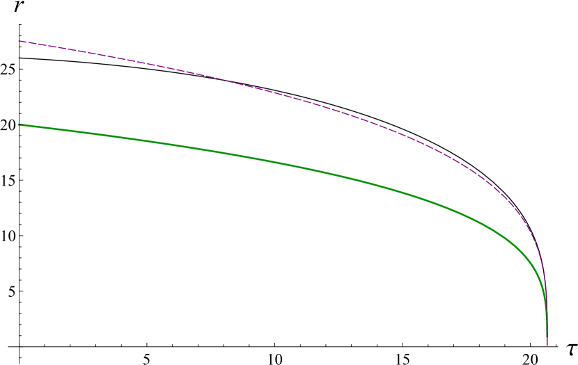
Figure 3: Timelike ZAMO geodesics on the equatorial plane ($\theta=\frac{\pi}{2}$) of retarded Kerr-Vaidya spacetime. The thin black line is a timelike geodesic. The solid green line and thin dashed purple line are the apparent horizon and the gap seperatrix, respectively. The mass evolves as $m(u)=10-0.05\,u$ and the angular momentum per mass is $a=0.1$. The initial conditions are $r(\tau=0)=26$, $u(\tau=0)=0$, $\phi(\tau=0)=0$, $\dot{r}(\tau=0)=-0.12.$

IV Kerr–Vaidya solutions with variable $a$

The assumption that $a=J/M=\mathrm{const.}$ is incompatible with the continuous eventual evaporation of a physical black hole, as for $M<a$ the equation $\Delta=0$ has no real roots and the Hawking temperature

$$T=\frac{1}{2\pi}\left(\frac{r_{0}-M}{r_{0}^{2}+a^{2}}\right)\ ,$$ (76)

which is proportional to the surface gravity, goes to zero as $M\to a$. Moreover, the semiclassical analysis [6] shows that during evaporation via Hawking radiation, $a/M$ decreases faster than $M$ [22, 23, 24].

Geometries with variable $M$ and $a$ are considerably more intricate. The Newman–Penrose formalism [4, 7] is based using a null tetrad, which consists of two real null vectors (such as $k_{\pm}^{\mu}=(e_{\hat{0}}^{\mu}\pm e_{\hat{1}}^{\mu})/\sqrt{2}$ that are constructed from the vectors given in Appendix B.2), and two complex conjugate null vectors that are constructed from a pair of real orthonormal spacelike vectors that are also orthogonal to the vectors $k^{\mu}_{\pm}$. The ten independent components of the Weyl tensor can be represented by five complex scalars, denoted as $\Psi_{0},\ldots,\Psi_{4}$. Subjecting the null tetrad to some Lorentz transformation is possible to have

$$\Psi_{0}\to\tilde{\Psi}_{0}=\Psi_{0}+4b\Psi_{1}+6b^{2}\Psi_{2}+4b^{3}\Psi 3+b^{4}\Psi_{4}\ ,$$ (77)

where $b$ is a complex scalar. The roots of the equation $\tilde{\Psi}_{0}=0$ play a crucial role in the algebraic classification of spacetimes. If the equation admits four distinct roots, the spacetime is classified as algebraically general; otherwise, it is algebraically special. Kerr–Vaidya metrics with $a=\mathrm{const.}$ is of type II, as Kerr metrics are. This is why these metrics posses principal null geodesic congruences and can be written in Kerr–Schild form. However, the metric with variable $a$ are of Petrov type I (algebraically general) and thus can not be cast into a Kerr-Schild form [39].

On the other hand, such metrics are still compatible with asymptotic flatness. Calculating components of the Riemann tensor in the Newman–Penrose formalism we find that in the limit $r\to\infty$ all components approach zero. For example, the Ricci scalar behaves as

$$R=\frac{ar(r^{2}(3\cos 2\theta+1)-a^{2}\cos^{2}\theta(\cos 2\theta-5))}{\rho^{6}}a^{\prime}(v)\\ +{\cal O}\left(a^{\prime 2}\right)\ .$$ (78)

The EMT $T^{{\hat{a}}}_{~{}~{}\hat{b}}$, written in an orthonormal basis, has four distinct Lorentz-invariant eigenvalues. Two eigenvalues are complex, and two are real, corresponding to spacelike eigenvectors. This observation implies that the EMT is type IV (see Appendix B.2.2 for details).

Variable $a$ introduces additional terms to the geodesic equations. In the advanced metrics the additional terms are finite. In the retarded metrics potentially the most divergent term contributing to the right hand side of Eq. (68) is

$$\delta\ddot{r}=\kappa aa^{\prime}\dot{u}^{2}+\mathcal{O}(\dot{u})\ ,$$ (79)

where

$$\kappa=\frac{2r(a^{2}+r^{2})M\left((a^{2}+r^{2})\rho^{2}\cos^{2}\theta+2r^{3}M\sin^{2}\theta\right)}{\rho^{6}\Sigma^{2}}>0\ .$$ (80)

If the evaporation does not stop until $M=a=0$, the divergence of Eq. (75) does not occur. However, as the signs of $a^{\prime}$ and $M^{\prime}$ coincide, the dynamics will be qualitatively similar to the Vaidya case.

V Rindler Horizons for Kerr–Vaidya black holes

The near-horizon geometry of a Schwarzschild black hole can be conformally mapped to a Rindler spacetime [6, 11, 40]

$$ds^{2}=-\epsilon^{2}dt^{2}+d\epsilon^{2}+dY^{2}+dZ^{2}\ ,$$ (81)

which has a horizon at $\epsilon=0$ (called the Rindler horizon) that separates the left and right Rindler wedge of Minkowski space. In the Rindler decomposition of Minkowski space, observers with constant proper acceleration $\mathfrak{a}$ follow orbits of the Lorentz boost operator $K$, and thus observe the Minkowski vacuum as a thermal density matrix at temperature $T_{U}=\mathfrak{a}/2\pi$ due to the presence of a Rindler horizon. In the Schwarzschild geometry, a local observer hovering at fixed areal radius near the event horizon requires a proper acceleration $\kappa\sim 1/4M$ with respect to the asymptotic frame in order to maintain their position. The corresponding Unruh temperature is then just $T_{U}=1/8\pi M$, which is precisely the Hawking temperature.

It is worth noting that despite this formal analogy, the Hawking and Unruh effects remain physically distinct. Spatial homogeneity of the Unruh temperature cannot be maintained for macroscopic objects [42], and the radiation is observed as an isotropic heat bath [43], while Hawking radiation is not. Even in the infinite mass limit (where one expects the Rindler approximation to the near-horizon region to become exact) the topological difference between the Schwarzschild and Rindler geometries enters as a difference in sub-leading factors for the entanglement entropy across the respective horizons [41].

Nonetheless, such a near-horizon Rindler approximation has considerable utility and has been used for computing black hole entropy [44], generalizing the laws of black hole mechanics [45], and in the study of asymptotic symmetries [46]. A similar relationship is expected to hold in a more general dynamical setting [40, 14], and has been shown to hold also for PBHs.

For the Vaidya black hole (a PBH with $w_{1}\approx 0$ in the notation of Sec. II.2) it has been shown that there a precise conformal transformation between the near-horizon geometry the Rindler space [47], allowing one to compute the associated Hawking temperature in the dynamical background. The general feature of black hole geometries admitting a Rindler/conformal Rindler description near their horizons allows one to associate yet another horizon to a black hole—the Rindler horizon. In the examples we discuss here, the Rindler horizon of a black hole coincides with the separatrix (the outgoing radial (ZAMO) null curve for which $d^{2}r/d\tau^{2}=0$). For black holes evolving adiabatically the separatrix very closely approximates the event horizon, making it a useful notion of horizon in the discussion of dynamical black hole evaporation [11, 14].

V.1 Case 1: constant $a$

The Schwarzschild-Rindler analogy described above can readily be extended to the axially symmetric case. To determine the location of the separatrix for the Kerr–Vaidya metric with constant $a$ we consider an outgoing null curve, which to leading order is given by

$$\dot{r}=\frac{\Delta}{2(r^{2}+a^{2})}\ ,$$ (82)

where we have chosen a parametrization such that $\tau=v$. Differentiation with respect to $\tau$ gives

$$\frac{d^{2}r}{d\tau^{2}}=\frac{(r\dot{r}-\dot{M}r-M\dot{r})(r^{2}+a^{2})-\Delta r\dot{r}}{(r^{2}+a^{2})^{2}}\ .$$ (83)

Using (82) and imposing the condition that $\frac{d^{2}R}{d\tau^{2}}=0$ then gives

$$\frac{d^{2}r}{d\tau^{2}}=\frac{(r\Delta-2M^{\prime}r(r^{2}+a^{2})-M\Delta)(r^{2}+a^{2})-\Delta^{2}r}{2(r^{2}+a^{2})^{3}}=0\ .$$ (84)

Keeping only the leading order terms in the near horizon expansion implies that

$$\Delta\approx\frac{2M^{\prime}r_{0}(r_{0}^{2}+a^{2})}{r_{0}-M}\ .$$ (85)

On the other hand, the Kerr–Vaidya metric can be written in the form

$$ds^{2}=-\frac{\Delta\rho^{2}\ d\tilde{v}^{2}}{(r^{2}+a^{2})^{2}}+\frac{2\rho^{2}\ d\tilde{v}dr}{r^{2}+a^{2}}+\rho^{2}(d\theta^{2}+\sin^{2}\theta d\tilde{\phi}^{2})\ ,$$ (86)

where

$$d\tilde{v} =\frac{(r^{2}+a^{2})}{\rho^{2}}\left(dv-a\sin^{2}\theta d\psi\right)\ ,$$ (87)

$$d\tilde{\phi} =\frac{(r^{2}+a^{2})}{\rho^{2}}\left(d\psi-\frac{a}{a^{2}+r^{2}}dv\right)\ .$$

$d\tilde{v}$ and $d\tilde{\phi}$ are the respective analogs of $dt$ and $d\psi$ of the Schwarzschild metric. This correspondence is almost exact with one exception: $d\tilde{v}$ and $d\tilde{\phi}$ together with $d\theta$ and $dr$ form an anholonomic basis of one-forms. This means that there are no globally defined coordinates $X$ and $\tilde{X}$ such that $d\tilde{v}$ = $dX$ and $d\tilde{\phi}=d\tilde{X}$. Near the hypersurface $r_{0}=M+\sqrt{M^{2}-a^{2}}$, we then make the following approximations:

$$\Delta=\frac{\gamma^{2}\tilde{\epsilon}^{2}}{4}+\gamma h(v) M^{\prime}\ ,\quad r-r_{0}=\frac{\gamma\tilde{\epsilon}^{2}}{4}+h(v)M^{\prime}\ ,$$

$$\gamma =2\sqrt{M^{2}-a^{2}}\ ,$$ (88)

where $h(v)$ is a function determining the location of Rindler horizon. Then the Kerr–Vaidya metric (33) reduces to

$$ds^{2} =-\frac{\rho_{0}^{2}}{r_{0}^{2}+a^{2}}\left[\left(\frac{\gamma h}{r_{0}^{2}+a^{2}}-2\left(1+\frac{2M}{\gamma}\right)\right)M^{\prime}\right.$$

$$\quad\left.+\frac{\gamma^{2}\tilde{\epsilon}^{2}}{4(r_{0}^{2}+a^{2})}\right]d\tilde{v}^{2}+\frac{\rho_{0}^{2}\gamma\tilde{\epsilon}}{r^{2}+a^{2}}d\tilde{v}d\tilde{\epsilon}$$ (89)

$$\quad+\rho_{0}^{2}\left(d\theta^{2}+\sin^{2}\theta d\tilde{\phi}^{2}\right)\ ,$$

where only terms up to order $\tilde{\epsilon}^{2}$ and $M^{\prime}$ have been retained. The function $h(v)$ is now chosen to be

$$h=\frac{4r_{0}(r_{0}^{2}+a^{2})}{\gamma^{2}}\ ,$$ (90)

which reduces the above metric to the form

$$ds^{2}=-\frac{\rho_{0}^{2}\gamma^{2}\tilde{\epsilon}^{2}\ d\tilde{v}^{2}}{4(r_{0}^{2}+a^{2})^{2}}+\frac{\rho_{0}^{2}\gamma\tilde{\epsilon}\ d\tilde{v}d\tilde{\epsilon}}{r_{0}^{2}+a^{2}}+\rho_{0}^{2}\left(d\theta^{2}+\sin^{2}\theta d\tilde{\phi}^{2}\right)\ ,$$ (91)

Finally, we make a further substitution

$$\rho d\tilde{\epsilon}=d\epsilon\ ,$$ (92)

which also implies that

$$d(\rho\tilde{\epsilon})\approx d\epsilon\ .$$ (93)

Substituting these relations into (91), we obtain

$$ds^{2}=-\frac{\gamma^{2}\epsilon^{2}\ d\tilde{v}^{2}}{4(r_{0}^{2}+a^{2})^{2}}+\frac{\gamma\epsilon\ d\tilde{v}d\epsilon}{r_{0}^{2}+a^{2}}+\rho_{0}^{2}(d\theta^{2}+\sin^{2}\theta d\tilde{\phi}^{2})\ .$$ (94)

This shows that the separatrix of a Kerr–Vaidya black hole, determined by (85), coincides with the Rindler horizon of the Kerr–Vaidya metric. In Ref. [47] it was shown that the location of the Rindler horizon plays a crucial role in determining the temperature of Hawking radiation in particular classes of dynamical spacetimes. This surface is also the null surface whose parameter rate of area change is constant. To see this, consider the second derivative $d^{2}A/d\tau^{2}$, where $A=4\pi(r^{2}+a^{2})$ is the surface area along a set of outgoing null rays, using the parametrization $\tau=v$ for null geodesics. The radial null vector for which $d^{2}A/dv^{2}=0$ coincides with that of Eq. (85) up to order ${\cal O}(M^{\prime})$. It remains to be seen whether this notion of horizon can play a useful role in generalizing the laws of black hole mechanics to a dynamical setting, where the degeneracy of different horizons is usually absent.

V.2 Case 2: variable $a$

We now determine the location of the separatrix for the ingoing Kerr–Vaidya metric with variable $a$. For this metric also, Eq. (82) holds. Now, we follow the exact same procedure outlined in the previous section to determine the location of the separatrix

$$\Delta=2\frac{M^{\prime}r_{0}-a^{\prime}a}{r_{0}-M}(r_{0}^{2}+a^{2})\ .$$ (95)

Now, to determine the location of the Rindler horizon, we perform the anholonomic coordinate transformations given in Eq. (87) to obtain the exact same metric of Eq. (86) (but with variable $a$). We then make the following approximations:

$$r-r_{0}=\frac{\gamma\tilde{\epsilon}^{2}}{4}+h(v)M^{\prime}+g(v)a^{\prime}\ ,$$ (96)

near the hypersurface $r_{0}=M+\sqrt{M^{2}-a^{2}}$, where $\gamma$ and $h(v)$ are defined in Eq. (88). Here $g(v)$ is an additional function depending on the location of the Rindler horizon. Then the Kerr–Vaidya metric with variable $a$ reduces to

$$ds^{2} =-\frac{\rho_{0}^{2}}{r_{0}^{2}+a^{2}}\left[\left(\frac{\gamma h}{r_{0}^{2}+a^{2}}-2\left(1+\frac{2M}{\gamma}\right)\right)M^{\prime}\right.$$

$$\quad\left.\left(\frac{\gamma g}{r_{0}^{2}+a^{2}}+\frac{4a}{\gamma}\right)a^{\prime}+\frac{\gamma^{2}\tilde{\epsilon}^{2}}{4(r_{0}^{2}+a^{2})}\right]d\tilde{v}^{2}$$ (97)

$$+\frac{\rho_{0}^{2}\gamma\tilde{\epsilon}}{r^{2}+a^{2}}d\tilde{v}d\tilde{\epsilon}\quad+\rho_{0}^{2}\left(d\theta^{2}+\sin^{2}\theta d\tilde{\phi}^{2}\right)\ ,$$

where only terms up to order $\tilde{\epsilon}^{2}$, $M^{\prime}$ and $a^{\prime}$ have been retained. The functions $h(v)$ and $g(v)$ are now chosen to be

$$h=\frac{4r_{0}(r_{0}^{2}+a^{2})}{\gamma^{2}},\quad g=-\frac{4a(r_{0}^{2}+a^{2})}{\gamma^{2}}\ ,$$ (98)

which reduces the above metric to the form

$$ds^{2}=-\frac{\rho_{0}^{2}\gamma^{2}\tilde{\epsilon}^{2}\ d\tilde{v}^{2}}{4(r_{0}^{2}+a^{2})^{2}}+\frac{\rho_{0}^{2}\gamma\tilde{\epsilon}\ d\tilde{v}d\tilde{\epsilon}}{r_{0}^{2}+a^{2}}+\rho_{0}^{2}\left(d\theta^{2}+\sin^{2}\theta d\tilde{\phi}^{2}\right)\ ,$$ (99)

Finally, we make a further substitution

$$\rho d\tilde{\epsilon}=d\epsilon\ \implies d(\rho\tilde{\epsilon})\approx d\epsilon\ ,$$ (100)

to obtain

$$ds^{2}=-\frac{\gamma^{2}\epsilon^{2}\ d\tilde{v}^{2}}{4(r_{0}^{2}+a^{2})^{2}}+\frac{\gamma\epsilon\ d\tilde{v}d\epsilon}{r_{0}^{2}+a^{2}}+\rho_{0}^{2}(d\theta^{2}+\sin^{2}\theta d\tilde{\phi}^{2})\ .$$ (101)

Hence, the location of the separatrix of a Kerr–Vaidya black hole with variable $a$ also coincides with the Rindler horizon.

VI Discussion

In our prior work [47, 20] we explored the use of the Vaidya metric as a consistent model of the near-horizon geometry of an evaporating black hole, in a semiclassical framework where back-reaction phenomena are implicitly accounted for. The issue of consistently incorporating back-reaction in fully dynamical settings, where solutions to the semiclassical Einstein equations are unavailable, remains open. However, we were able to show that some of the expected features of dynamical black holes can nonetheless be consistently modelled, and the physical criteria explicit in their construction dramatically constrains their properties.

In this work we considered the class of Kerr–Vaidya spacetimes as a minimal axially symmetric model for the near-horizon region, based on the fact that (non-rotating) Vaidya metrics provide a self-consistent near-horizon description of physical black holes in the spherical symmetric case. We find that explicit violation of the null energy condition inherent in the Kerr–Vaidya metric is compatible with the expected properties of Hawking emission when back-reaction on the geometry is present. The Kerr–Vaidya solutions which represent evaporating black holes possess timelike apparent horizons. Infalling observers on geodesic trajectories experience no drama during their approach and crossing of the horizon, and may reverse direction if their proper velocity is sufficiently small. Finite NEC violation occurs for infalling test particles which cross the horizon, and in the case of growing black hole energy density as measured by Alice will typically be positive. For evaporating black holes it is possible to communicate with the outside world from the apparent horizon and also parts of the trapped region outside the hypersurface $\Delta=0$. This is not so for accreting black holes. In fact, so long as the growth is continuous, the apparent horizon is hidden from outside observers.

On the contrary, we identify previously unappreciated issues with evaporating white hole geometries. We show that in both the outgoing Vaidya and outgoing Kerr–Vaidya metrics with decreasing mass function may have timelike geodesics reach the singularity while starting outside of any horizons present. In spherical symmetry this property is not a challenge to the cosmic censorship conjecture, since the relevant solutions may be dismissed as unphysical (due to impossibility of their realisation in finite time according to a distant observer).

For Kerr–Vaidya black holes both with constant and variable angular momentum to mass ratio $a$, we also showed that two distinct notions of horizon become equivalent in the near-horizon description. The separatrix of the Kerr–Vaidya geometry (which approximates the event horizon when $M^{\prime}\ll M^{\prime 2}$) was shown to coincide precisely with the location of the Rindler horizon. This horizon plays a crucial role in the Hawking evaporation of a Kerr–Vaidya black hole, in accordance with previous work which used the Rindler form of the Kerr–Vaidya metric to determine the associated Hawking temperature. This suggests that the Kerr–Vaidya metric serves as a consistent model capturing back-reaction due to the Hawking process.

Like with the spherically symmetric Vaidya metric, the Kerr–Vaidya metric is expected only to provide an accurate description near the horizon, where the flux due to Hawking evaporation is ingoing and of negative energy density. In the far region, evaporation produces a positive outgoing flux, and a more complete characterization of the geometry necessitates the use of multiple Kerr–Vaidya metrics. We leave the problem of generalizing such multi-Vaidya models to axially symmetric and cosmological spaces to future investigations.

Appendix A Spherically-symmetric solutions in $(u,r)$ coordinates

A.1 Basic properties

A useful relationship between the EMT components $T_{\mu\nu}$ in $(t,r)$ coordinates and $\Theta_{\mu\nu}$ in $(u,r)$ coordinates is given by

$${\theta}{{}_{u}}\vcentcolon=e^{-2h_{-}}{\Theta}_{uu}={\tau}{{}_{t}},$$ (102)

$${\theta}_{ur}\vcentcolon=e^{-h_{-}}{\Theta}_{ur}=\left({\tau}{{}_{t}^{r}}+{\tau}{{}_{t}}\right)/f,$$ (103)

$${\theta}{{}_{r}}\vcentcolon={\Theta}_{rr}=\left({\tau}{{}^{r}}+{\tau}{{}_{t}}+2{\tau}{{}_{t}^{r}}\right)/f^{2},$$ (104)

where similarly to the Schwarzschild coordinate setting we introduced the effective EMT components $\theta_{a}$, $a=u,r,ur$. The Einstein equations can then be written as

$${\partial}_{u}C_{-}=8\pi r^{2}\Theta^{r}_{\;u}=-8\pi r^{2}e^{h_{-}}({\theta}{{}_{u}}-f{\theta}_{ur}),$$ (105)

$${\partial}_{r}C_{-}=8\pi r^{2}\Theta^{u}_{\;u}=-8\pi r^{2}{\theta}_{ur},$$ (106)

$${\partial}_{r}h_{-}=-4\pi re^{h_{-}}\Theta^{u}_{\;r}=4\pi r{\theta}{{}_{r}}.$$ (107)

Tangent vectors to the congruences of outgoing and ingoing radial null geodesics are given in $(u,r)$ coordinates by

$$l_{+}^{\mu}=(0,e^{-h_{-}},0,0),\qquad l_{-}^{\mu}=(1,-{\tfrac{1}{2}}e^{h_{-}}f,0,0),$$ (108)

respectively. The vectors are normalized to satisfy $l_{+}\cdot l_{-}=-1$. Their expansions are

$$\vartheta_{+}=\frac{2e^{-h_{-}}}{r},\qquad\vartheta_{-}=-\frac{e^{h_{-}}f}{r},$$ (109)

respectively. Hence the (outer) anti-trapping horizon is located at the Schwarzschild radius $r_{\textsl{g}}$, justifying the definition of the white hole mass as $2M(u)=r_{-}(u)$.

We focus now on Vaidya solutions as they capture all the near-horizon features of solutions of the same type. The four-velocity of a radially moving observer Alice is

$$u^{\mu}_{\mathrm{A}}=\big{(}\dot{u},\dot{r},0,0\big{)},$$ (110)

and the spatial outward-pointing unit vector normal to it is

$$n^{\alpha}=(-\dot{u},f\dot{u}+\dot{r},0,0,).$$ (111)

If $\dot{r}^{2}\gg f$, then expanded in terms of $z=r-r_{-}$ gives

$$\dot{u}=-2\dot{r}\frac{r_{-}}{z}+\mathcal{O}\big{(}z^{0}\big{)},$$ (112)

for ingoing observers if $z\ll r_{-}$, and

$$\dot{u}\approx-\frac{2\dot{r}}{1-\chi_{+}\alpha}=-\frac{\dot{r}}{\alpha}+\mathcal{O}(\alpha)$$ (113)

for the linear evaporation law with $\alpha<1/8$ (See Appendix A.2). On the other hand,

$$\dot{u}=\frac{1}{2\dot{r}^{2}}+\mathcal{O}(z),$$ (114)

for outgoing observers.

The only nonzero EMT component is $T_{uu}=-r^{\prime}_{-}/(8\pi r^{2})$, and thus Alice’s locally measured energy density, pressure and flux are

$$\varrho_{\mathrm{A}}=-\varphi_{\mathrm{A}}=p_{\mathrm{A}}=-\frac{r^{\prime}_{-}(u)\dot{u}^{2}}{8\pi r^{2}}\ .$$ (115)

Then using Eq. (114) we obtain Eq. (25), while for the ingoing observer with $\dot{r}^{2}\gg f$ Eq. (112) gives

$$\varrho_{\mathrm{A}}=-\varphi_{\mathrm{A}}=p_{\mathrm{A}}=-\frac{r^{\prime}_{-}(u)\dot{r}^{2}}{2\pi z^{2}}+\mathcal{O}\big{(}z^{-1}\big{)}.$$ (116)

A.2 Timelike geodesics in retarded Viadya spacetimes with decreasing mass

By adapting the analysis of [49] to $(u,r)$ coordinates with $r^{\prime}_{-}<0$ the diagrams of Fig. 2 can be explicitly calculated, as the metric of Eq. (27) with $r_{-}^{\prime}=-\alpha$ possesses a conformal Killing vector

$$\xi^{\mu}=-\alpha(u,r,0,0)\ ,$$ (117)

satisfying

$$\mathcal{L}_{\xi}g_{\mu\nu}=2g_{\mu\nu}\ .$$ (118)

We assume that the evaporation is completed at $u=0$, and we have

$$r_{-}=-\alpha u\ ,\quad 0>u>u_{0}\ ,$$ (119)

during the evaporation. At the first stage we introduce new retarded and radial coordinates,

$$\eta=-\ln(-u)\ ,\quad\chi=-\frac{u}{r}\ ,$$ (120)

transforming the metric to

$$ds^{2}=e^{-2\eta}\left[-\left(1-\alpha\chi-\frac{2}{\chi}\right)d\eta^{2}+\frac{2}{\chi^{2}}d\eta d\chi+\frac{1}{\chi^{2}}d\Omega_{2}\right]\ .$$ (121)

The advanced null coordinate is defined as

$$\zeta=\eta+2\chi_{*}\ ,$$ (122)

where the relation

$$\chi_{*}=\frac{1}{\chi\left(2\mu\chi^{2}-\chi+2\right)}d\chi\ ,$$ (123)

is chosen to eliminate the diagonal term $d\eta^{2}$. In the double null coordinates

$$ds^{2}=-e^{-2\eta}\left(1-\alpha\chi-\frac{2}{\chi}\right)d\eta d\zeta+\frac{e^{-2\eta}}{\chi^{2}}d\Omega_{2}\ ,$$ (124)

where $\chi$ is an implicit function of $\eta$ and $\zeta$. The component $\textsl{g}_{\zeta\eta}$ has zeroes that define the conformal Killing horizons — null surfaces of co-dimension one where the norm of $\xi$ vanishes and to which $\xi$ is orthogonal. They are located at ($z_{\pm}$ in the notation of [49])

$$\chi_{\pm}=\frac{1\pm\sqrt{1-8\alpha}}{2\alpha},\quad\text{ for $0<\alpha\leq\frac{1}{8}$}\ .$$ (125)

Extension of the null geodesics along the lines of constant $\eta$ leads to the three blocks on Fig. 2(b), while the case $\alpha>1/8$ results in Fig. 2(b). Matching the horizon $\eta_{+}$ for $u<u_{0}$ with an eternal white hole, however, requires either some domain of a continuous transition or emission of a (infinitesimally) thin shell of finite mass.

Horizon crossing is avoided (at least temporarily, as it happens for expanding PWHs), if $\dot{z}>0$. At later stages of the infall into an evaporating Vaidya white hole $|\dot{r}|\gg|\dot{z}|\sim 0$, while its initial behaviour depends on the initial data and parameters of the solution. Using that $z\approx z_{*}$ at the last stages before the divergence of $\dot{r}$, we can improve the bound of Eq. (32),

$$|\ddot{r}|>\frac{2|r^{\prime}_{-}|\dot{r}^{2}}{rf^{2}}>\frac{2|r^{\prime}_{-}|\dot{r}^{2}}{r},$$ (126)

in the case of constant $r_{-}^{\prime}=-\alpha$. Using Eq. (112) we have

$$|\ddot{r}|>\frac{\dot{r}^{2}}{2\alpha(1+\epsilon)^{2}r}\ ,$$ (127)

where $\epsilon\lesssim 1$ for sufficiently small $z\gg r_{-}$. For a linear evaporation law we reach the same conclusion using Eq. (113), even if $r\approx r_{+}\sim r_{-}$.

The equation

$$\ddot{r}=-\frac{\beta\dot{r}^{2}}{r}\ ,$$ (128)

where $0<\beta=\mathrm{const}$ has an exact solution. Taking $\beta=1/(2\alpha)$ and the initial conditions $r(0)=r_{\mathrm{in}}>0$ and $\dot{r}(0)=\dot{r}_{\mathrm{in}}<0$ results in

$$r=r_{\mathrm{in}}\left(\frac{2\alpha r_{\mathrm{in}}}{|\dot{r}_{\mathrm{in}}|}-(1+2\alpha)\tau\right)^{\frac{2\alpha}{1+2\alpha}}\left(\frac{|\dot{r}_{\mathrm{in}}|}{2\alpha r_{\mathrm{in}}}\right)^{\frac{2\alpha}{1+2\alpha}},$$ (129)

where the radial velocity diverges when

$$\tau_{*}=\frac{2\alpha r_{\mathrm{in}}}{|\dot{r}_{\mathrm{in}}|(1+2\alpha)}\ .$$ (130)

The approximation above gives a good estimate of when the system of the geodesic equations breaks down. If the usual semiclassical evaporation law applies, the evaporation rate $|r_{-}^{\prime}|$ is an increasing function of time and Eq. (32) indicates that the runaway solutions are possible.

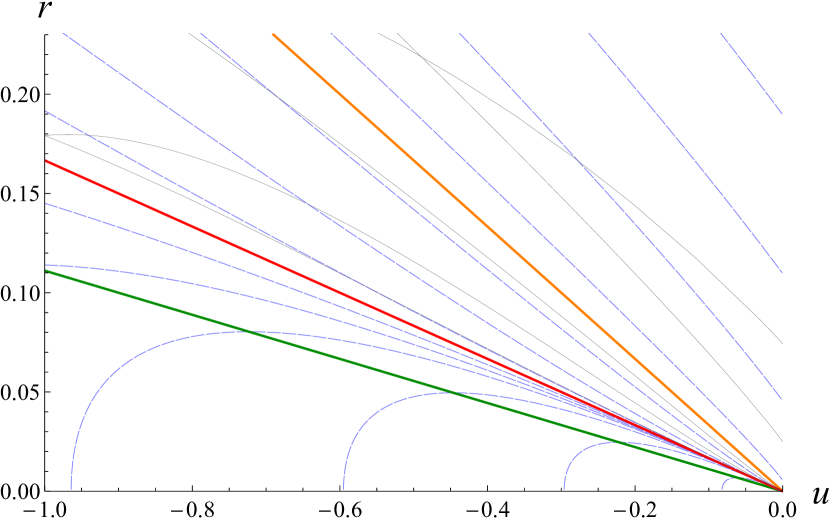
Figure 4: Geodesics of the retarded Vaidya spacetime with linear evaporation law $r_{-}=-\alpha u$ and $\alpha=\frac{1}{9}<\frac{1}{8}$. The conformal Killing Horizons $\chi_{\pm}$ are shown as the straight lines $r_{\pm}=-u/\chi_{\pm}$ in red and orange, respectively. The green line is the anti-trapping horizon. Several typical ingoing null (blue lines) and ingoing and outgoing timelike geodesics (black lines) are shown. The outgoing null geodesics $u=\mathrm{const.}$ are not shown as not to clutter the figure.

Numerical simulations show that for a wide range of initial conditions, after a finite interval of Alice’s proper time she experiences a flash of energy, as

$$\varrho_{\mathrm{A}}=T_{\mu\nu}u^{\mu}_{\mathrm{A}}u^{\nu}_{\mathrm{A}}=\frac{\alpha}{r}\dot{u}^{2}\to\infty\ .$$ (131)

For the linear evaporation law the suitable initial locations are at $r_{+}(u_{\mathrm{in}})<r_{\mathrm{in}}<r_{-}(u_{\mathrm{in}})$. Moreover, some initially outgoing trajectories suffer the same fate (Fig. 4). This occurs for general evaporation laws, including the standard $r^{\prime}_{-}\propto r_{-}^{-2}$, as shown on Fig. 5. However, note that these divergences occur at the endpoint of evaporation, where the Vaidya approximation to the evaporating white hole geometry is no longer expected to be valid anyway.

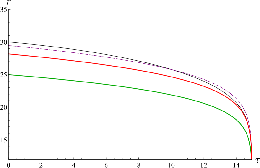
Figure 5: Timelike geodesics of the retarded Vaidya spacetime: Thin black line is a timelike geodesic. Solid red line, solid green line and thin dashed purple line are the inner conformal Killing horizon, the anti-trapping horizon and the gap seperatrix respectively. The apparent horizon follows a linear evaporation law, $r_{-}=r_{-}^{0}-\alpha u$ where $r_{-}^{0}=25$ and $\alpha=2\mu=0.05<\frac{1}{8}$. The initial conditions are $r(\tau=0)=30$, $u(\tau=0)=0$, $\dot{r}(\tau=0)=-0.22.$

Appendix B Kerr–Vaidya metrics

B.1 Expansions of the outgoing and ingoing Vaidya metric

Here we focus on the black hole solutions using the $(v,r)$ coordinates. Expansions of the outgoing and the ingoing geodesics that are tangent to the normals to the hypersurface $\Delta=0$

$$l^{+}_{\mu}= \frac{\rho^{2}}{2\Sigma^{2}}\big{(}-\Delta,r^{2}+a^{2}+\Sigma,0,0\big{)},$$ (132)

$$l^{-}_{\mu}= \big{(}-1,(r^{2}+a^{2}-\Sigma)/\Delta,0,0\big{)},$$ (133)

have the expansions

$$\vartheta_{+}= \frac{1}{2\Sigma^{3}}\bigg{(}\Delta(2r\rho^{2}+a^{2}\sin^{2}\theta(M+r))$$

$$+M^{\prime}ra^{2}\sin^{2}\theta(r^{2}+a^{2}+\Sigma)\bigg{)}\ ,$$ (134)

$$\vartheta_{-}= -\frac{1}{\Sigma\rho^{2}}\bigg{(}2r\rho^{2}+a^{2}\sin^{2}\theta(M+r)$$

$$+\frac{r^{2}+a^{2}-\Sigma}{\Delta}M^{\prime}ra^{2}\sin^{2}\theta\bigg{)}\ ,$$ (135)

respectively [38]. This identifies the Kerr–Vaidya solutions as black holes and indicate that the trapped region extends beyond $\Delta=0$ in the evaporating case. Its boundary as described in Eq. (47) can be determined using the expansions of the pair of outward- and inward- pointing future-directed null vector orthogonal to the $u=\text{constant}$ hypersurface and the two-surface $r_{0}+M^{\prime}\varsigma(v,\theta)$ that (before the rescaling) are given by [35]

$$\ell^{\pm}_{\mu}\propto(-1,\ell_{\pm},-\ell_{\pm}M^{\prime}{\partial}_{\theta}\varsigma,0)\ .$$ (136)

The null condition $l^{\pm}\cdot l^{\pm}=0$ gives

$$l^{\pm}=\frac{1}{\Delta+(M^{\prime}{\partial}_{\theta}\varsigma)^{2}}\Big{(}r^{2}+a^{2}\pm\sqrt{\Sigma^{2}-(aM^{\prime}{\partial}_{\theta}\varsigma)^{2}\sin^{2}\theta}\,\Big{)}\ .$$ (137)

B.2 Energy-momentum tensor

B.2.1 Kerr–Vaidya metrics

The non-zero components of the EMT for the Kerr–Vaidya metric (33) in advanced coordinates are

$$T_{vv}=\frac{r^{2}(a^{2}+r^{2})-a^{4}\cos^{2}\theta\sin^{2}\theta}{4\pi\rho^{6}}M_{v}-\frac{a^{2}r\sin^{2}\theta}{8\pi\rho^{4}}M_{vv}\ ,$$ (138)

$$T_{v\theta}=-\frac{a^{2}r\sin\theta\cos\theta}{4\pi\rho^{4}}M_{v},$$ (139)

$$T_{v\psi}=-a\sin^{2}\theta T_{vv}-a\sin^{2}\theta\frac{r^{2}-a^{2}\cos^{2}\theta}{8\pi\rho^{4}}M_{v}\ ,$$ (140)

$$T_{\theta\psi}=\frac{a^{3}r\sin^{3}\theta\cos\theta}{4\pi\rho^{4}}M_{v}\ ,$$ (141)

$$T_{\psi\psi}=a^{2}\sin^{4}\theta T_{vv}+a^{2}\sin^{4}\theta\frac{r^{2}-a^{2}\cos^{2}\theta}{4\pi\rho^{4}}M_{v}\ .$$ (142)

Likewise, the non-zero components of the EMT for the Kerr–Vaidya metric (34) in retarded coordinates are

$$T_{uu}=-\frac{r^{2}(a^{2}+r^{2})-a^{4}\cos^{2}\sin^{2}\theta}{4\pi\rho^{6}}M_{u}-\frac{a^{2}r\sin^{2}\theta}{8\pi\rho^{4}}M_{uu}\ ,$$ (143)

$$T_{u\theta}=-\frac{2a^{2}r\sin\theta\cos\theta}{8\pi\rho^{4}}M_{u},$$ (144)

$$T_{u\psi}=-a\sin^{2}\theta T_{uu}+a\sin^{2}\theta\frac{r^{2}-a^{2}\cos^{2}\theta}{8\pi\rho^{4}}M_{u}\ ,$$ (145)

$$T_{\theta\psi}=\frac{2a^{3}r\sin^{3}\theta\cos\theta}{8\pi\rho^{4}}M_{u}\ ,$$ (146)

$$T_{\psi\psi}=a^{2}\sin^{4}\theta T_{uu}-a^{2}\sin^{4}\theta\frac{(r^{2}-a^{2}\cos^{2}\theta)}{4\pi\rho^{4}}M_{u}\ .$$ (147)

In advanced coordinates the decomposition (42) of the EMT is obtained using the vectors

$$k_{\mu}=(1,\;0,\;0,\;-a\sin^{2}\theta),\$$ (148)

and

$$q_{\mu}=\bigg{(}0,\;0,\;T_{v\theta},\;-a\sin^{2}\theta\frac{r^{2}-a^{2}\cos^{2}\theta}{8\pi\rho^{4}}M_{v}\bigg{)}.$$ (149)

The orthonormal tetrad for which $k^{\mu}=e_{\hat{1}}^{\mu}+e_{\hat{0}}^{\mu}$ is given by

$$e_{\hat{0}}^{\mu}=(-1,rM/\rho^{2},0,0)\ ,$$ (150)

$$e_{\hat{1}}^{\mu}=(1,1-rM/\rho^{2},0,0)\ ,$$ (151)

$$e_{\hat{2}}^{\mu}=(0,0,1/\rho,0)\ ,$$ (152)

$$e_{\hat{3}}^{\mu}=\frac{1}{\rho}\big{(}a\sin\theta,a\sin\theta,0,\csc\theta\big{)}\ .$$ (153)

Hence the EMT is given by Eq. (44) with

$$\nu=T_{vv}\ ,\qquad q^{\mu}=q^{\hat{2}}e_{\hat{2}}^{\mu}+q^{\hat{3}}e_{\hat{3}}^{\mu}\ ,$$ (154)

where

$$q^{\hat{2}}= -\frac{a^{2}rM_{v}}{8\pi\rho^{5}}\sin 2\theta\ ,$$ (155)

$$q^{\hat{3}}= {-\frac{a(r^{2}-a^{2}\cos^{2}\theta)M_{v}}{8\pi\rho^{5}}\sin\theta\ .}$$ (156)

B.2.2 Variable $a$

If we regard the angular momentum per unit mass as a function of time variable, the resulting Kerr–Vaidya metric would not be asymptotically flat. Although the general form of the EMT is not informative, we can take the limit as $r\to\infty$ to study the asymptotic behaviour of the EMT of such a spacetime. For the ingoing Kerr–Vaidya metric the non-zero components are

$$T_{v\phi} =-\frac{1}{2}\sin^{2}\theta a^{\prime\prime}(v)\ ,$$ (157)

$$T_{\theta\theta} =\frac{1}{16}\left(16a\sin^{2}\theta a^{\prime\prime}(v)+12\sin^{2}\theta a^{\prime}(v)^{2}\right)\ ,$$ (158)

$$T_{\phi\phi} =\frac{1}{8}\left(8a\sin^{4}\theta a^{\prime\prime}(v)+2\sin^{4}\theta a^{\prime}(v)^{2}\right)\ .$$ (159)

Let $T^{{\hat{a}}\hat{b}}$ be the EMT in an orthonormal frame defined by Eqs. (150)-(153) with $a=a(v)$. The Lorentz-invariant eigenvalues are then the roots of the equation

$$\det(T^{{\hat{a}}\hat{b}}-\lambda\eta^{{\hat{a}}\hat{b}})=0,\qquad\eta^{{\hat{a}}\hat{b}}=\mathrm{diag}(-1,1,1,1)\ .$$ (160)

For the above EMT we have four distinct eigenvalues, two of which are real and two of which are complex. As the general forms of the eigenvalues are lengthy, we show explicit expressions for two of the real eigenvalues around the equatorial plane. They are given by

$$\lambda^{(1)}= \frac{\mathfrak{l}^{1/3}}{3^{2/3}r^{8}}-\frac{r^{3}a^{\prime}(v)\left((4M+r)a^{\prime}(v)+2aM^{\prime}(v)\right)}{(3\chi)^{1/3}}\ ,$$ (161)

$$\lambda^{(2)}= -\frac{aa^{\prime}(v)}{r^{3}},$$ (162)

where subleading terms of order ${\cal O}(M^{\prime 2},a^{\prime 2})$ have been discarded and we have defined

$$\mathfrak{l} =9r^{21}a^{\prime}(v)^{2}M^{\prime}(v)+9r^{19}aa^{\prime}(v)^{2}\left(2Ma^{\prime}(v)+aM^{\prime}(v)\right)$$

$$\quad+\bigg{[}3r^{38}a^{\prime}(v)^{3}\bigg{(}27a^{\prime}(v)\left(2aMa^{\prime}(v)+\left(a^{2}+r^{2}\right)M^{\prime}(v)\right)^{2}$$

$$\quad+r\left(a^{\prime}(v)(4M+r)+2aM^{\prime}(v)\right)^{3}\bigg{)}\bigg{]}^{1/2}\ .$$ (163)

In the most general scenario, there exist four distinct eigenvalues, with two of them being complex. The remaining two eigenvalues are real and correspond to spacelike eigenvectors. As a result, we have no real timelike or null eigenvectors. This implies that the EMT is of type IV. The real spacelike eigenvector is $e_{\hat{2}}^{\mu}$ corresponding to the eigenvalue $\lambda^{(2)}$. Similarly, the spacelike eigenvector corresponding to the eigenvalue $\lambda^{(1)}$ is

$$\bigg{(}1,1-\dfrac{\lambda^{(1)}r^{4}a^{\prime}(v)}{\zeta},0,\dfrac{-\lambda^{(1)2}r^{6}}{\zeta}\bigg{)}\ ,$$ (164)

where

$$\zeta =a^{\prime}(v)\left(\lambda^{(1)}r^{3}(2M+r)-2\left(a^{2}+r^{2}\right)M^{\prime}(v)\right)$$

$$\quad-4aMa^{\prime}(v)^{2}+\lambda^{(1)}r^{3}aM^{\prime}(v)\ .$$ (165)

On the other hand, the Kerr–Vaidya metric with $a=\mathrm{const.}$ is of type III because it has one null and one spacelike eigenvector with quadruple degenerate eigenvalue $\lambda^{4}=0$.

B.3 Geodesics of Kerr–Vaidya spacetimes

Here we summarise some useful facts about timelike geodesics in the ingoing Kerr–Vaidya metrics. The Lagrangian of a massive test particle is

$$ds^{2}= \frac{1}{2}\left[\bigg{(}1-\frac{2Mr}{\rho^{2}}\bigg{)}\dot{v}^{2}-2\dot{v}\dot{r}-\frac{4aMr\sin^{2}\theta}{\rho^{2}}dvd\psi\right.$$

$$\left.-2a\sin^{2}\theta drd\psi\!+\rho^{2}d\theta^{2}+\frac{\Sigma^{2}}{\rho^{2}}\sin^{2}\theta d\psi^{2}\right]\ .$$ (166)

The Lagrange equations of motion is

$$\frac{d}{d\tau}\left(\frac{\partial L}{\partial\dot{x}^{\mu}}\right)-\frac{\partial L}{\partial x^{\mu}}=0\ ,$$ (167)

which for $r$ component becomes

$$-\frac{1}{2}\frac{d}{d\tau}(\dot{v}-a\sin^{2}\theta\dot{\psi})-\frac{\partial L}{\partial r}=0\ .$$ (168)

Substituting the ZAMO condition (49) and simplifying further gives

$$-\frac{1}{2}\frac{d}{d\tau}\left(\frac{\rho^{2}}{\Sigma^{2}}\big{(}(r^{2}+a^{2})\dot{v}-a^{2}\sin^{2}\theta\dot{r}\big{)}\right)-\frac{\partial L}{\partial r}=0\ .$$ (169)

Similarly, $v$ component of the Lagrangian equations of motion becomes

$$-\frac{1}{2}\frac{d}{d\tau}\left(\dot{r}-\left(1-\frac{2Mr}{\rho^{2}}\right)\dot{v}-\frac{2aMr\sin^{2}\theta}{\rho^{2}}\dot{\psi}\right)-\frac{\partial L}{\partial v}=0\ .$$ (170)

Again substituting ZAMO condition (63) and simplifying further gives

$$\frac{1}{2}\frac{d}{d\tau}\left(\frac{\rho^{2}}{\Sigma^{2}}\big{(}\Delta\dot{v}-(r^{2}+a^{2})\dot{r}\big{)}\right)-\frac{\partial L}{\partial v}=0\ .$$ (171)

Multiplying Eq. (169) by $\Delta$ and Eq. (171) by $r^{2}+a^{2}$ and adding the equations eliminates the $\ddot{v}$ terms, allowing one to obtain the expression for $\ddot{r}$ in terms of first derivatives only

$$\left(\dot{v}\Delta\frac{d}{d\tau}(r^{2}+a^{2})-(r^{2}+a^{2})\dot{v}\frac{d\Delta}{d\tau}-\Delta\dot{r}\frac{d}{d\tau}(a^{2}\sin^{2}\theta)+(r^{2}+a^{2})\dot{r}\frac{d}{d\tau}(r^{2}+a^{2})+\Sigma^{2}\ddot{r}\right)\frac{\rho^{2}}{\Sigma^{4}}\\ +\dot{r}\frac{d}{d\tau}\left(\frac{\rho^{2}}{\Sigma^{2}}\right)-\Delta\frac{\partial L}{\partial r}-(r^{2}+a^{2})\frac{\partial L}{\partial v}=0\ .$$ (172)

Analysis of the leading order terms near the horizon shows that the acceleration is negative and decreasing as the particle goes outward from the expanding black hole:

$$\ddot{r}\approx-\frac{4r\left(a^{2}+r^{2}\right)M^{\prime}(v)}{\Delta^{2}}\dot{r}^{2}+{\cal O}(1/\Delta)\ .$$ (173)

Following the same procedure for the evaporating white hole shows that the acceleration is negative and increasing as the particle approaches the evaporating white hole:

$$\ddot{r}\approx\frac{4r\left(a^{2}+r^{2}\right)M^{\prime}(u)}{\Delta^{2}}\dot{r}^{2}+{\cal O}(1/\Delta)\ .$$ (174)

References

- [1] V. Cardoso and P. Pani, Living Rev. Relativ. 22, 4 (2019).
- [2] L. Barack, V. Cardoso, S. Nissanke, and T. P. Sotiriou, Class. Quant. Grav. 36, 143001 (2019).
- [3] S. W. Hawking and G. F. R. Ellis, The Large Scale Structure of Space-Time (Cambridge University Press, Cambridge, England, 1973).
- [4] S. Chandrasekhar, The Mathematical Theory of Black Holes (Oxford University Press, Oxford, England, 1992).
- [5] B. O’Neil, The Geometry of Kerr Black Holes, (Peters, Wellesley, MA, 1995).
- [6] V. P. Frolov and I. D. Novikov, Black Holes: Basic Concepts and New Developments (Kluwer, Dordrecht, 1998).
- [7] H. Stephani, D. Kramer. M. MacCallum, C. Hoenselaers, and E. Herlt, Exact Solutions to Einstein’s Field Equations (Cambridge University Press, Cambridge, England, 2003).
- [8] E. Poisson, A Relativist’s Toolkit (Cambridge University Press, Cambridge, England, 2004).
- [9] V. Faraoni, Cosmological and Black Hole Apparent Horizons, (Springer, Heidelberg, 2015).
- [10] K. Kiefer, Quantum Gravity, Third Edition (Oxford University Press, Oxford, 2012).
- [11] R. Brout, S. Massar, R. Parentani, and P. Spindel, Phys. Rep. 260, 329 (1995).
- [12] R. B. Mann, Black Holes: Thermodynamics, Information, and Firewalls (Springer, New York, 2015).
- [13] E.-A. Kontou and K. Sanders, Class. Quant. Grav. 37, 193001 (2020).
- [14] R. B. Mann, S. Murk, and D. R. Terno, Int. J. Mod. Phys. D 31, 2230015 (2022).
- [15] R. B. Mann, S. Murk, and D. R. Terno, Phys. Rev. D 105, 124032 (2022).
- [16] P. K. Dahal, S. Murk and D. R. Terno, AVS Quantum Sci. 4, 015606 (2022).
- [17] R. V. Vasudevan et al. Mon. Not. R. Astron. Soc. 458, 2012 (2016).
- [18] J. Jiang, et al., Mon. Not. R. Astron. Soc. 477, 3711 (2018).
- [19] J. Roulet, M. Zaldarriaga, Mon. Not. R. Astron. Soc. 484, 4216 (2019).
- [20] P. K. Dahal, F. Simovic, I. Soranidis, I., and D. R. Terno, [arXiv:2303.15793 [gr-qc]].
- [21] F. Fayos and R. Torres, Class. Quant. Grav. 25, 175009 (2008).
- [22] D. N. Page, Phys. Rev. D 13, 198 (1976).
- [23] R. Dong, W. H. Kinney and D. Stojkovic, J. Cosmol. Astropart. Phys. 10 034 (2016).
- [24] A. Arbey, J. Auffinger, and J. Silk, Mon. Not. R. Astron. Soc. 494, 1257 (2020).
- [25] N. Dadhich, A. Tursunov, B. Ahmedov and Z. Stuchlík, Mon. Not. R. Astron. Soc. Lett. 478, L89 (2018).
- [26] V. Faraoni, G. F. R. Ellis, J. T. Firouzjaee, A. Helou, and I. Musco, Phys. Rev. D 95, 024008 (2017).
- [27] D. R. Terno, Phys. Rev. D 100, 124025 (2019).
- [28] C. Barcelo, S. Liberati, S. Sonego and M. Visser, Phys. Rev. D 77, 044032 (2008).
- [29] S. Murk and I. Soranidis, Phys. Rev. D 108, 044002 (2023).
- [30] V. Baccetti, R. B. Mann, S. Murk, and D. R. Terno, Phys. Rev. D 99, 124014 (2019).
- [31] P. K. Dahal, I. Soranidis, and D. R. Terno, Phys. Rev. D 106, 124048 (2022).
- [32] R. M. Wald and S. Ramaswamy, Phys. Rev. D 21, 2736–2741 (1980).
- [33] V. Baccetti, R. B. Mann, and D. R. Terno, Class. Quant. Grav. 35, 185005 (2018).
- [34] C. González, L. Herrera, and J. Jiménez, J. Math. Phys. 20, 837 (1979).
- [35] P. K. Dahal and D. R. Terno, Phys. Rev. D 102, 124032 (2020).
- [36] M. Murenbeeld and J. R. Trollope, Phys. Rev. D 1, 3220 (1970).
- [37] D.-Y. Xu, Class. Quant. Grav. 16, 343 (1999).
- [38] J. M. M. Senovilla and R. Torres, Class. Quant. Grav. 32, 189501 (2015).
- [39] T. Christoulakis, T. Grammenos and C. Kolassis, Phys. Lett. 149A, 354 (1990).
- [40] T. Padmanabhan, Gravity and the Spacetime: An Emergent Perspective, in A. Ashtekhar and V. Petkov, Springer Handbook of Spacetime (Springer Berlin, Heidelberg, 2014).
- [41] S. N. Solodukhin, Living Rev. Relativ. 14, 8 (2011).
- [42] D. Buchholz and R. Verch, Class. Quant. Grav. 32, 245004 (2015).
- [43] U. H. Gerlach, Phys. Rev. D 27, 2310 (1983).
- [44] G. Cognola, L. Vanzo and S. Zerbini, Class. Quantum Grav. 12, 1927 (1995).
- [45] E. Bianchi and A. Satz, Phys. Rev. D 87, 124031 (2013).
- [46] H. Chung, Phys. Rev. D 82, 044019 (2010).
- [47] P. K. Dahal and F. Simovic, [arXiv:2304.11833 [gr-qc]]
- [48] K. Jusufi, Gen. Relativ. Grav. 50 84 (2018).
- [49] W. A. Hiscock, L. G. Williams, and D. M. Eardley, Phys. Rev. D 26, 751 (1982).