Modeling blazar broadband emission with convolutional neural networks - I. Synchrotron self-Compton model

Abstract

Modeling the multiwavelength spectral energy distributions (SEDs) of blazars provides key insights into the underlying physical processes responsible for the emission. While SED modeling with self-consistent models is computationally demanding, it is essential for a comprehensive understanding of these astrophysical objects. We introduce a novel, efficient method for modeling the SEDs of blazars by the mean of a convolutional neural network (CNN). In this paper, we trained the CNN on a leptonic model that incorporates synchrotron and inverse Compton emissions, as well as self-consistent electron cooling and pair creation-annihilation processes. The CNN is capable of reproducing the radiative signatures of blazars with high accuracy. This approach significantly reduces computational time, thereby enabling real-time fitting to multi-wavelength datasets. As a demonstration, we used the trained CNN with MultiNest to fit the broadband SEDs of Mrk 421 and 1ES 1959+650, successfully obtaining their parameter posterior distributions. This novel framework for fitting the SEDs of blazars will be further extended to incorporate more sophisticated models based on external Compton and hadronic scenarios, allowing for multi-messenger constraints in the analysis. The models will be made publicly available via a web interface, the Markarian Multiwavelength Datacenter, to facilitate self-consistent modeling of multi-messenger data from blazar observations.

1 Introduction

Blazars are a subclass of active galactic nuclei which have their jet oriented at a small angle relative to the observer’s line of sight (Blandford & Rees, 1978; Urry & Padovani, 1995). Due to this orientation and the relativistic nature of their jets, blazars exhibit exceptional observational features, such as a high luminosity, strong polarization, and rapid, high-amplitude variability. The bolometric luminosity of blazars can reach up to $10^{48}\>{\rm erg.s^{-1}}$ (e.g., Beckmann & Shrader, 2012), making them the most powerful non-explosive objects in the Universe. Their extreme luminosity enables the detection of blazars even at high redshifts (e.g., Rau et al., 2012; Ackermann et al., 2017; Sahakyan et al., 2020, 2023b).

Blazars are commonly classified into two major types based on their optical emission lines. The blazars having bright and broad emission lines with equivalent widths of ${\rm|EM|>}$ 5 Å are classified as Flat Spectrum Radio Quasars (FSRQs). In contrast, when the emission lines are weak or absent, they are identified as BL Lacertae objects (BL Lacs). While these two subclasses share many observational similarities, the difference in line emission suggests that different physical mechanisms are responsible for generating their broadband emissions.

The broadband emission of blazars spans from radio frequencies to the high-energy $>100$ MeV, and even to the very high-energy $>100$ GeV) $\gamma$-ray bands, exhibiting a typical dual-bump shape (e.g., Padovani et al., 2017). The low-energy component, observed from the radio through the optical/X-ray bands, is commonly attributed to synchrotron radiation produced by electrons accelerated in the jet which is supported by the observed high degree of polarization (e.g., Beckmann & Shrader, 2012). However, the origin of the second component, which extends above the X-ray band, continues to be a subject of discussion. In a leptonic scenario, this HE component is attributed to inverse Compton scattering of low-energy photons by the same energetic electrons responsible for the synchrotron radiation. These low-energy photons could either be synchrotron photons produced within the jet itself (synchrotron self-Compton (SSC) model, see e.g., Ghisellini et al., 1985; Maraschi et al., 1992; Bloom & Marscher, 1996; Tavecchio et al., 1998), or they could have an external origin (external Compton (EC) model, see e.g., Dermer et al., 1992; Dermer & Schlickeiser, 1994; Sikora et al., 1994; Błażejowski et al., 2000; Dermer et al., 2009; Ghisellini & Tavecchio, 2009; Sikora et al., 2009). These two alternative radiation mechanisms are also further used to explain the differences between FSRQs and BL Lac, respectively associated to EC and to SSC models.

Hadronic models provide another explanation of the second component: it can either be from the direct synchrotron emission from protons that are co-accelerated with electrons (Mücke & Protheroe, 2001), or it can arise from secondary particles generated through photo-pion and photo-pair interactions (see e.g. Mannheim, 1993; Mannheim & Biermann, 1989; Mücke & Protheroe, 2001; Mücke et al., 2003; Böttcher et al., 2013; Petropoulou & Mastichiadis, 2015; Gasparyan et al., 2022). In this case, neutrino emission is also expected, making blazars attractive targets for multi-messenger astrophysical studies. The attention to the hadronic models has grown, particularly following the observation of IceCube-170922A, a neutrino event which was detected from the direction of the blazar TXS 0506+056 (IceCube Collaboration et al., 2018a, b; Padovani et al., 2018). Various models have then been applied to explain both the broadband spectral and the neutrino emission from individual blazars ( e.g., Ansoldi et al., 2018; Keivani et al., 2018a; Murase et al., 2018; Sahakyan, 2018; Righi et al., 2019; Cerruti et al., 2019; Sahakyan, 2019; Gao et al., 2019; Gasparyan et al., 2022; Sahakyan et al., 2023a).

Blazars are monitored across various wavelengths, leading to the accumulation of a substantial volume of multi-wavelength data over different time periods and many numerical codes have been developed to model this wealth of data. Some of these codes focus exclusively on leptonic interactions. This is the case of, e.g., naima (Zabalza, 2015), JetSeT (Tramacere et al., 2009, 2011; Tramacere, 2020), agnpy (Nigro et al., 2022). Both leptonic and hadronic interactions are included in e.g., AM3 (Gao et al., 2017), ATHE$\nu$A (Mastichiadis & Kirk, 1995), Böttcher13 (Böttcher et al., 2013) LeHa-Paris (Cerruti et al., 2015), LeHaMoC Stathopoulos et al. (2023) and SOPRANO (Simulator of Processes in Relativistic AstroNomical Objects, Gasparyan et al., 2022). These codes make different assumptions, employ different methodologies, include various physical processes, and while some operate under the steady state assumption, others are time-dependent.

For this paper, we used the kinetic code SOPRANO. SOPRANO is a fully conservative and implicit kinetic code designed to compute the radiative signatures of accelerated leptons and hadrons, taking into account a broad range of physical processes as well as time-dependent cooling mechanisms for both primary and secondary particles. In SOPRANO, the energy discretization is based on the discontinuous Galerking method, and the time-stepping can either be first order or exponential first order, in case of steep problems. Written in C for speed and highly optimized, SOPRANO is used via a python wrapper. This allowed us to perform the 200k simulations required for this project. SOPRANO has been successfully applied to model the multi-messenger spectral energy distributions (SEDs) of TXS 0506 + 056 (Gasparyan et al., 2022), PKS 0735+178 (possibly in association with several neutrino events, Sahakyan et al., 2023a), and Mrk 501 (Abe et al., 2023) during the historically low X-ray and $\gamma$-ray state.

Over the years, the complexity of models has dramatically increased with the inclusion of more physical mechanisms to explain numerous observed features and details. For instance, including radiative contributions from protons to account for VHE neutrinos, along with the consideration of particle decay and cooling as they radiate, has led to computationally intensive models, which prevent parameter explorations and the interpretation of the data through model fitting. As a result, fitting blazar SEDs is possible only with ’simple’ models. For example, in Sahakyan (2021); Sahakyan & Giommi (2022); Sahakyan et al. (2022), blazar SEDs observed during different periods are modeled with JetSeT (Tramacere, 2020). Their analysis assumed an ad hoc electron distribution function, and although this approach allows for estimating the evolution of parameters over time, it does not include electron cooling. So it remains unclear whether such an ad hoc electron distribution can be formed. Alternatively when computationally intensive models are built, they are typically superimposed onto data from a specific celestial object. In such cases, obtaining statistical information about model parameters becomes infeasible due to the prohibitive computational cost of model evaluation.

Recent attempts to compare multi-messenger sets of data, including particle cooling and interactions have also been made. However, among other challenges, these approaches necessitate tremendous computational resources, questioning their use on large sample and time-resolved SED modeling. For instance, Finke et al. (2008) uses a recursive strategy to attempt to converge towards the best fit parameters. A similar method, although modified, was also used in Petropoulou et al. (2015). Instead Ahnen et al. (2017) used a grid-scan strategy to model the SED of Mrk 501. Rodrigues et al. (2023) also relied on a strategy of grid scanning to find the best parameters, working in a hierarchical way from the simplest leptonic model to the most complicated hadronic models by adding components and freezing the parameters of the previous sub-models. With this approach, no model comparison can be performed and the reliability of the parameter distributions is impacted by the lack of cross-correlation between the parameters at different levels, even if in the last stage a global likelihood minimization is performed. Their study extracts parameters from 324 blazars but requires a computational cost of approximately 17 thousand node-hours, which, to our understanding, cannot be reused for blazars outside of the original sample.

Another recent example is the work of Stathopoulos et al. (2023), who introduced LeHaMoC, a versatile lepto-hadronic code capable of computing spectra in just a few seconds. This speed enabled the authors to fit the SED of the blazar HSP J095507.9+355101. However, as acknowledged by Stathopoulos et al. (2023), the computational time required still prohibits the use of Markov Chain Monte Carlo (MCMC) fitting for blazar SEDs. The computational time for LeHaMoC is somewhat comparable to that of SOPRANO (Gasparyan et al., 2022), leading us to the same conclusion: current computational resources do not permit a systematic comparison between model and data, nor do they allow for thorough constraints on model parameters and their study.

We are therefore at a crossroad where we either continue to rely on simple models or we find a solution that allows the use of computationally intensive complex models for the analysis and fitting of blazar SEDs. The objective of this paper is to introduce a new methodology that addresses this challenge by integrating complex and resource-intensive numerical models in detailed comparisons with data. Our method uses convolutional neural network (hereafter CNN), a specific type of feed-forward neural network that efficiently calculates the resulting spectrum from a given set of model parameters with high accuracy, requiring approximately a millisecond. This makes it well-suited for complex fitting procedures. Although the creation of the set of spectra required to train the CNN demands considerable computational resources, once trained for a specific model, the CNN can be cost-effectively deployed for the interpretation of any blazar SED.

In this paper, we train our CNN on a sample of spectra numerically obtained from an SSC model of blazars, using SOPRANO (Gasparyan et al., 2022). We subsequently employ the trained CNNs to fit the broadband SEDs of Mrk 421 and 1ES 1959+650 in order to demonstrate its performance. The paper is organized as follows: In section 2, we review the SSC model and outline the numerical methods implemented in SOPRANO for computing the resulting spectra. Section 3 presents our numerical table model, detailing the range of model parameters and validating the computed spectra. Section 4 describes the CNN, providing insights into the training procedure and the measures taken to prevent spurious oscillations in the spectra generated by the CNN. Section 5 applies the CNN to the analysis of the SEDs of blazars Mrk 421 and 1ES 1959+650 performed in the Bayesian framework. Our conclusions are summarized in section 6.

2 The model: synchrotron self-Compton

Parameter	Units	Symbol	Minimum	Maximum	Type of distribution
Doppler boost	-	$\delta$	3	50	Linear
Blob radius	cm	R	$10^{15}$	$10^{18}$	Logarithmic
Minimum electron injection Lorentz factor	-	$\gamma_{\rm min}$	$10^{1.5}$	$10^{5}$	Logarithmic
Maximum electron injection Lorentz factor	-	$\gamma_{\rm max}$	$10^{2}$	$10^{8}$	Logarithmic
Injection index	-	$p$	$1.8$	5	Linear
Electron luminosity	erg.s-1	$L_{e}$	$10^{42}$	$10^{48}$	Logarithmic
Magnetic field	G	$B$	$10^{-3}$	$10^{2}$	Logarithmic

Table 1: Characteristics of the dataset. For each parameter, we recall its unit (if any) and symbol, and we provide its range and the distribution of the discreet parameter values. The total number of spectra is set to $2\times 10^{5}$.

In this paper, we focus on modeling the emission from BL Lacs within the framework of the SSC model, for which the low-energy bump is attributed to the synchrotron emission of relativistic electrons, while the second peak arises from the inverse Compton scattering of the synchrotron photons on the same electron population. This model successfully reproduces the observed multiwavelength spectrum as well as the observational features in different bands, and is widely adopted for modeling the observed data from optical to the VHE $\gamma$-ray bands.

In the one-zone SSC model, it is assumed that the emission originates from a spherical region of the jet (referred to as a ’blob’) with a comoving radius $R$, which moves with Lorentz factor $\Gamma$. We assume that the observers sees the jet at angle $1/\Gamma$, such that the Doppler boost factor $\delta\equiv\Gamma$. The magnetic field $B$ inside this region is assumed to be homogeneous and constant. Electrons, once injected into this region, lose their energy under the effect of the magnetic field as well as by interacting with the local photon fields, ultimately generating the observed broadband spectrum.

Despite the likely presence of protons in the jet, for the SSC model, we assume that only electrons are accelerated and radiate once injected in the radiation zone. The injection function $Q_{e}$ is assumed to be a cutoff power-law with index $p$ for electrons with a Lorentz factor $\gamma$ larger than a minimum Lorentz factor $\gamma_{\rm min}$, such that

$$Q_{e}=\left\{\begin{aligned} &Q_{e,0}\gamma^{-p}\exp\left(-\frac{\gamma}{\gamma_{\max}}\right)&&\gamma\geq\gamma_{\rm min},\\ &0&&{\rm otherwise.}\end{aligned}\right.$$ (1)

where $\gamma_{\rm max}$ is the cutoff electron Lorentz factor. The normalization $Q_{e,0}$ is set so that the electron luminosity $L_{e}$ is determined by

$$L_{e}=\pi R^{2}\delta^{2}m_{e}c^{3}\int_{1}^{\infty}\gamma Q_{e}d\gamma,$$ (2)

where $m_{e}$ is the electron rest mass and $c$ is the speed of light. The temporal evolution of the electron distribution is obtained by solving the Fokker-Planck diffusion equation, while the evolution of photons is described by an integro-differential equation. We label the distribution function of photons by $N_{\gamma}$, and that of electrons by $N_{e}$. With the photon energy denoted as $x$, the kinetic equations are

$$\left\{\begin{aligned} \frac{\partial N_{e}}{\partial t}(\gamma)&=\frac{N_{e}}{t_{\rm esc}}+\frac{\partial}{\partial\gamma}\left[(C_{\rm IC}N_{\gamma}+C_{\rm sync})N_{e}\times\right]+Q_{\gamma\gamma\rightarrow e^{+}e^{-}},\\ \frac{\partial N_{\gamma}}{\partial t}(x)&=\frac{N_{\gamma}}{t_{\rm esc}}+Q_{\rm sync}+R_{\rm IC}N_{\gamma}-S_{\gamma\gamma\rightarrow e^{+}e^{-}},\end{aligned}\right.$$ (3)

where $t_{\rm esc}=t_{\rm dyn}=R/c$ is the escape time, such that the first term on the right hand side of each equation represent the escape of particles from the radiation zone, $C_{\rm IC}$ and $C_{\rm sync}$ represent inverse Compton and synchrotron cooling, $Q_{\gamma\gamma\rightarrow e^{+}e^{-}}$ and $S_{\gamma\gamma\rightarrow e^{+}e^{-}}$ are the source and sink terms associated to pair creation respectively, and $R_{\rm IC}$ is the redistribution kernel of Compton scattering. We note here that we do not include synchrotron self-absorption in our analysis as it is not yet included into SOPRANO. More details on the kinetic equations and their numerical solutions are given in Gasparyan et al. (2022), which also provides the expressions for all the rates that appear in these equations.

In this paper, we employ SOPRANO (Gasparyan et al., 2022) to solve the set of coupled kinetic equations as defined in Equation 3. We obtain the equilibrium solution to the kinetic equations (3) by evolving the system in time until $t=4t_{\rm dyn}=4R/(\delta c)$. Our experiences show that further time evolution does not significantly alter the distribution functions; hence, we designate these as equilibrium distributions. These distributions serve as the final output from SOPRANO and are subsequently used to train the CNN.

3 Numerical model: computation and validation

In this section, we provide details of the methodologies employed in our study to simulate spectra, which will be used as inputs to the CNN. Namely, we give details on the parameter space used for generating the SEDs via SOPRANO. With regards to the large number of spectra, we also provide our methodology to assess the validity of the generated spectra.

3.1 Parameter ranges and sampling

For the SSC model considered in this paper, there are seven free parameters: the comoving blob radius $R$, the Doppler factor of the emission region $\delta$, the comoving magnetic field strength $B$ within the emission zone, the electron luminosity $L_{e}$, the minimum Lorentz factor $\gamma_{\text{min}}$, the cutoff Lorentz factor $\gamma_{\text{max}}$, and the power-law index $p$. These parameters are inputs to SOPRANO which computes the resulting spectrum in a time frame ranging from several tens of seconds to a few minutes. This computational demand makes direct fits impossible due to the necessity to evaluate the model tens of thousands of times for a single fit. To overcome this challenge, we developed a CNN, which we trained on a set of $2\times 10^{5}$ spectra computed by SOPRANO. The input parameters cover the whole range of parameters relevant for an SSC model for any blazars. The calculation of so many spectra was facilitated by coupling SOPRANO as the spectrum generator with ronswanson—a python-based code designed for High-Performance Computing systems—as the distribution software (Burgess, 2023). The code ronswanson provides a flexible and comprehensive interface for constructing table models from computationally intensive simulations.

The ranges and sampling distributions for the model parameters are detailed in Table 1. The Doppler boost factor varies linearly between 3 and 50, and the power-law index $p$ is sampled linearly within the range of 1.8 to 5. We note that steep values of $p>3$ are not expected from theory of shock acceleration or magnetic reconnection (see e.g. Kirk et al., 2000; Sironi & Spitkovsky, 2011; Uzdensky, 2022). They are included so the range of $p$ is sufficiently large to not have to deal with boundaries. Alternatively, our method allows to set $p$ or to specify an informative prior, which can only be achieved if the model is trained on larger than expected range of the index. In contrast, the other model parameters, i.e the emission radius $R$, the minimum and maximum Lorentz factors $\gamma_{\rm min}$ and $\gamma_{\rm max}$, the electron luminosity $L_{e}$, and the strength of the comoving magnetic field $B$, are sampled logarithmically within their respective ranges, such that $15<\log(R)<18$, $1.5<\log(\gamma_{\rm min})<5$, $2<\log(\gamma_{\rm max})<8$, $42<\log(L_{e})<48$ and $-3<\log(B)<2$. This large range of the parameters guaranties that the CNN we developed will be usable for the modeling of any blazar SED.

We use Latin hypercube sampling to select the parameters of the spectra to be computed with SOPRANO (see e.g. McKay et al., 2000; Viana, 2016). This sampling method is a widely popular technique in the creation of surrogate models as it presents several advantages. First, it allows to specify the number of simulations to be computed. As a byproduct, this method does not require to specify parameter spacing. Second, it ensures uniform sampling across all parameters. Lastly, it avoids the regular sampling of parameters, which is typical in grid scan techniques. This variability in the sampling enhances the performance of the CNN, see e.g. Kamath (2022).

3.2 Properties and validation of the computed spectra

In this section, we discuss the computational performance of SOPRANO, assessing the reliability of the computed spectra. Given that it is impossible to individually verify each of the $2\times 10^{5}$ computed spectra, we rely on the meta-data taken for each simulations to assess the overall reliability of our numerical model. We anticipate that future implementations involving more complex models of blazar SEDs, such as external Compton or hadronic models, will necessitate even larger datasets. The validation methodology developed here will be applied in these future cases. In particular, we study (i) the time to solution ensuring it aligns with our expectations and prior experience with SOPRANO, (ii) the maximum error of the Newton-Raphson scheme over a simulation, and (iii) the number of times this maximum was larger than the targeted uncertainty in the computation, here set to $10^{-15}$.

First, we begin by analyzing the computational time required by SOPRANO for each run. The left panel of Figure 1 shows the the histogram of the run times for all simulations. The average simulation time is 43.7s per spectra, with a long tail extending beyond 700 seconds. These extended durations correspond to spectra characterized by a high compactness with small radius $R$, large electron luminosity $L_{e}$ and small injection Lorentz factor $\gamma_{\rm min}$. We further note that these computation times are obtained when each independent simulations is executed on 8 cores on a AMD EPYC 7713 64-Core Processor CPU. An average computation time of $\sim 40$s for evolving the spectra until 4$t_{\rm dyn}$ aligns with our initial expectations and previous experience with SOPRANO. Overall the computation of the table model with $2\times 10^{5}$ spectra required $\sim 20$ thousands core hours, which is feasible by any dedicated server in a couple of weeks. Although it remains a moderately expensive computation, our approach present the advantage that it needs to only be performed once, if the full parameter space relevant for blazar modeling in the SSC scenario is covered.

The computation of the spectra by SOPRANO can fail, specifically in regions of large compactness, for which the numerical integrator currently used is not adapted. These failures originate from the implicit nature of the integration scheme, which necessitates to find the root of a non-linear systems of equations. This solution is obtained with the Newton-Raphson root finding algorithm, which can, in some instances, not converge towards the solution with the required accuracy. For the current numerical model, the accuracy of the root solver is set at $10^{-15}$, close to machine accuracy. Yet, even if the required accuracy is not reached, the photons and electrons spectra are returned and the computation continued. Therefore, we computed the number of failures for each spectral computation as well as the maximum relative error on the solution.

The total number of spectra with at least one failed time iteration is 3693, constituting less than 2% of all calculated spectra. The distribution of the number of failed time bins per simulation is depicted in the right panel of Figure 1. The distribution of the maximum error across a full simulation is shown in the middle panel of Figure 1. It is evident that only a small fraction of the spectra are unreliable, with most spectra having a maximal error below $10^{-10}$. We verified that the unreliable spectra are in the range of parameters space which are irrelevant for the interpretation of blazar SED.

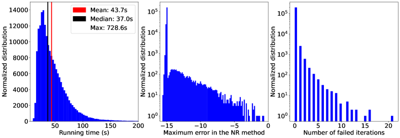
Figure 1: Left panel: distribution of the computation time for all simulations in the table model. The average compute time is $43.7$s while the median time is $37$s. Middle panel: Distribution of the maximum error in the Newton-Raphson method over the course of one simulation. We note that the ordinate is in logarithmic scale. Most of the spectra achieve the targeted relative error of $10^{-15}$. On the other hand, the computation of a small fraction of spectra (1.8%) is seen to fail with a larger error. Right panel: number of failed time iteration by simulations, which is 0 for most of our simulations, while less than 1.8 % of our simulations have a number of failures larger than 0.

4 Convolutional Neural Network

We initially attempted to directly use a table model by performing multi-dimensional linear interpolation between the intput parameters to evaluate the model for any given parameter set. However, we encountered limitations in the interpolation procedure in a critical region of the spectrum, specifically at the transition between the synchrotron and SSC components. Even increasing the number of points in the table model to several millions did not resolve this issue. This transition frequently occurs in the X-ray band and must be accurately represented for detailed analysis. Furthermore, the accurate modeling of this transition is also crucial in scenarios where neutrinos could be produced, as it constrains the maximum proton luminosity (e.g., see Gasparyan et al., 2022; Sahakyan et al., 2023a; Keivani et al., 2018b; Stathopoulos et al., 2022).

To address the challenge of fitting blazar SEDs, we have developed a surrogate model utilizing a CNN. In essence, the CNN is modeling the relationship between input parameters and their corresponding spectra. Our CNN is designed to reproduce the spectra from SOPRANO in 150 energy bins. Before performing the training, the input parameters are detrended and their mean removed. We follow the same receipt for the spectra. However, instead of considering the 150 output independent, the mean and variance are computed for all outputs across all generated spectra. This is an essential step because these outputs are not truly independent: they collectively form a consistent spectrum. Based on our experience and trials, treating the averages and means as independent variables leads to less accurate reconstructions. Furthermore, if each output is considered independently of the other, unwanted oscillations appear in the produced spectra. This is because if each values are independent, each one can overestimate or underestimate the spectrum independently of each other. To remove these oscillations, we introduce three linear combinations that link together the 150 spectral outputs within the model, by constraining linear combinations of local neighbors. These combinations are chosen to represent the finite difference derivative at order 2 and 8, as well as the finite difference of the second order derivative at order 4. In other words, our output vector is of length 586 where

• the first 150 outputs represent the targeted spectral output,

• the next 142 outputs represent the $8^{\rm th}$ order finite difference of the first derivative, multiplied by a numerical coefficient $d_{8}^{1}$ namely

  $$\frac{df_{i}}{d\epsilon} =d_{8}^{1}\left[\frac{f_{i-4}}{280}-\frac{4f_{i-3}}{105}+\frac{f_{i-2}}{5}-\frac{4f_{i-1}}{5}\right.$$ (4)

  $$\left.~{}~{}~{}~{}~{}~{}~{}~{}~{}~{}+\frac{4f_{i+1}}{5}-\frac{f_{i+2}}{5}+\frac{4f_{i+3}}{105}-\frac{f_{i+4}}{280}\right]$$

• the next 148 outputs represent the 2nd order finite difference approximation of the first derivative, multiplied by the coefficient $d_{2}^{1}$, namely

  $$\frac{df_{i}}{d\epsilon}=d_{1}^{1}\left[-f_{i-1}+f_{i-1}\right]$$ (5)

• the last 146 outputs represent the 4th order finite difference approximation of the second derivative, multiplied by the coefficient $d_{4}^{2}$ namely

  $$\frac{df_{i}}{d\epsilon}=d_{4}^{2}\left[-\frac{f_{i-2}}{12}+\frac{4f_{i-1}}{3}-\frac{5f_{i}}{2}+\frac{4f_{i+1}}{3}-\frac{f_{i+2}}{12}\right]$$ (6)

The CNN computes the 150 initial spectral outputs, and the remaining linear combinations are added in a last linear step. We find that setting the normalisation coefficients to $d_{4}^{1}=10$, $d_{2}^{1}=2$, and $d_{4}^{2}=4$ provides an adequate balance between (i) learning rate, (ii) accuracy of the CNN and (iii) the smoothness of the solution, specifically characterized by the absence of oscillatory behavior in the output spectra. We actually found that this method also increases the learning rate and the accuracy of the CNN.

By recursively building the CNN, we have determined that a deep network is not necessary to produce an accurate representation of our numerical model, which is computed using SOPRANO. Indeed, our CNN contains only 8 layers in this order: a first dense layer transform the 7 inputs to a high dimensional vector, 5 1D convolutional layer with different kernel size and stride, one maxpooling layer followed by a 1D convolutional layer and a final dense layer, mapping to the 150 outputs. This final layer of length 150 is then multiplied by the (non-square) matrix converting the 150 outputs to all outputs including the derivatives expressions. In this layer, all coefficients are known.

All these layers are followed by a ReLU activation function, apart from the maxpooling layer which is not followed by any, and the last dense linear layer, which is coupled to an activation function of type hyperbolic tangent.

In total our CNN comprises 687,815 free model parameters and is implemented using PyTorch. Our sample of spectra is split into a 80% training set, a 10% validation set and a 10% test set. We also experimented with different splits, but the results remain the same. The optimization is carried out via the NAdam algorithm, employing an epoch-dependent learning rate: $10^{-3}$ for the first 50 epochs, $10^{-4}$ for the subsequent 50 epochs, and $10^{-5}$ for the remaining 250 epochs. We use the L1 norm as our loss function with a sum reduction type. We find that our CNN model is straightforward to train and produces accurate results. Our CNN performances are attested by several metric scores applied on the validation set. With the inclusion of derivative expressions, the average $R^{2}$ score is $0.84$ where the average is taken across all resulting spectral point plus derivatives, the mean squared error (MSE) is $0.0004$, the mean absolute error (MAE) is $0.0027$ and the root mean squared error (RMSE) is $0.004$. In contrast, omitting the derivatives from the final score yields an average $R^{2}$ score of $0.9960$, an MSE of $9.4374\times 10^{-6}$, a MAE of $0.0013$, and an RMSE of $9.4374\times 10^{-6}$, all of which attest to the excellent performance of our CNN.

In Fig. 2, the two leftmost columns display representative examples of $\nu F_{\nu}$ spectra from the training set. They are superposed with their corresponding spectra as computed by the CNN. In contrast, the two rightmost columns of Fig. 2 feature spectra from the validation set, that is to say that were not used to train the CNN. These are also compared with their respective spectra generated by our CNN for comparative analysis. Despite a wide spread in normalization, the agreement between the original SOPRANO spectra and their corresponding CNN-generated spectra is remarkably high, spanning multiple orders of magnitude in both power and frequency. Notably, key features such as the synchrotron peak and the inverse Compton peak are accurately reproduced, once more attesting to the accuracy of the CNN model in reproducing the complex spectra produced from SOPRANO.

We note that the accuracy for some spectra is lower than for others. For instance, the second and third spectra on the second line is slightly off around frequency $10^{20}$Hz. We find that this happens at the boundary of the parameter space, as there is less information for the model to be train. On the other hand, these parameters are not expected to be relevant for the analysis of blazar SED, but have to be included to form regular continuous and independent parameter distributions.

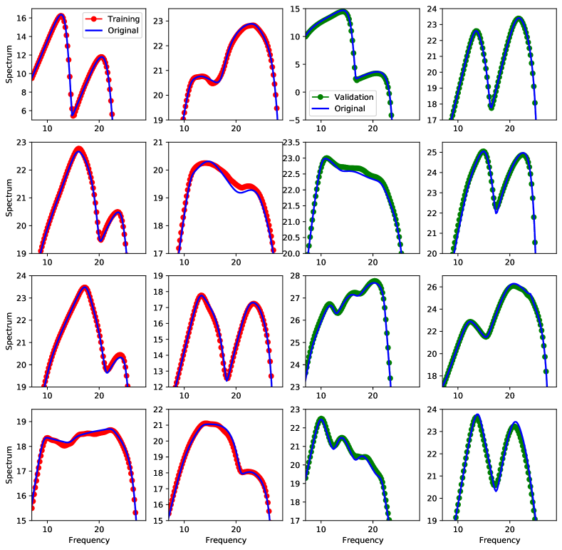
Figure 2: Comparison between the $\nu F_{\nu}$ spectra computed by the CNN (dotted line) and by SOPRANO (solid line) before unit conversion and expression in the observer frame. The x axis is the comoving frequency in unit of Hz. Left Panel: Spectra from the training set. Right Panel: Analogous spectra from the validation set. This figure shows the large diversity of spectra the CNN must be (and is) able to reproduce, the accuracy at which it reproduces them and the wide spam of the typical emitted power across the leptonic SSC model.

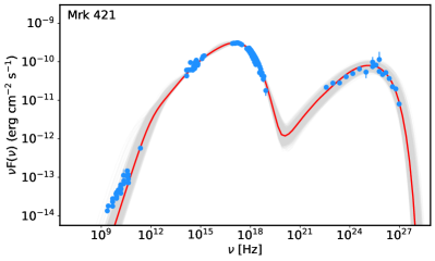
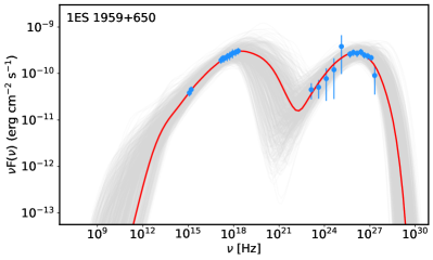
Figure 3: The broadband SEDs of Mrk 421 during the 4.5-month-long multi-wavelength campaign in 2009 (left) and of 1ES 1959+650 on the 14^th of June 2016 (right). The data and its errors are in blue, the red line is the model corresponding to the best parameters, i.e., maximizing the likelihood, and the grey spectra represent one in 10 randomly selected samples from the MCM sampling, representing the model uncertainty. The data are corrected for EBL absorption.

Table 2: Parameters describing the SEDs in Fig. 3 and 4. The two middle columns correspond to models with all 7 parameters free, while in the rightmost column, $R$ and $\delta$ are linked through the variability time.

Parameters	Mrk 421	1ES 1959+650	1ES 1959+650
$p$	$2.16\pm 0.08$	$2.26\pm 0.16$	$2.12\pm 0.14$
$\log_{10}(\gamma_{\rm max})$	$4.87\pm 0.16$	$6.41\pm 0.45$	$5.85\pm 0.48$
$\log_{10}(\gamma_{\rm min})$	$2.49\pm 0.22$	$3.20\pm 0.69$	$1.56\pm 0.68$
$\delta$	$31.01\pm 8.08$	$22.49\pm 9.54$	$40.03\pm 5.69$
$\log_{10}(B/[\rm G])$	$-1.17\pm 0.28$	$-1.62\pm 0.38$	$-0.72\pm 0.23$
$\log_{10}(R/[\rm cm])$	$16.43\pm 0.44$	$16.82\pm 0.38$	$15.44$
$\log_{10}(L_{\rm e}/[\rm erg\>s^{-1}])$	$43.32\pm 0.18$	$43.71\pm 0.32$	$43.41\pm 0.19$
$\log_{10}(L_{\rm B}/[\rm erg\>s^{-1}])$	$43.08$	$42.68$	$42.13$
	All parameters free	All parameters free	Variability time constraint

5 Modeling the broadband SEDs of Mrk 421 and 1ES 1959+650

To demonstrate the efficieny of our approach based on CNN in fitting and interpreting the SEDs of blazars, we model in this section the observed broadband dataset of two well-studied sources namely, Markarian 421 (Mrk 421) and 1ES 1959+650. Our analysis assumes uniform priors for the electron index $p$ and the Doppler boost $\delta$, and log-uniform priors for all remaining parameters, namely $R$, $B$, $L_{e}$, $\gamma_{\rm min}$, $\gamma_{\rm max}$. We assume a Gaussian likelihood and sample the posterior distributions with MultiNest (Feroz et al., 2009), a nested sampling algorithm designed for efficient Bayesian inference. We assume 1000 active points and a tolerance of $0.5$ to ensure efficient sampling and convergence. MultiNest offers a number of advantages, including computational efficiency and the ability to robustly handle multi-modal posterior distributions, which is a distinct possibility given the high dimensionality and complexity of the parameter space.

5.1 Markarian 421

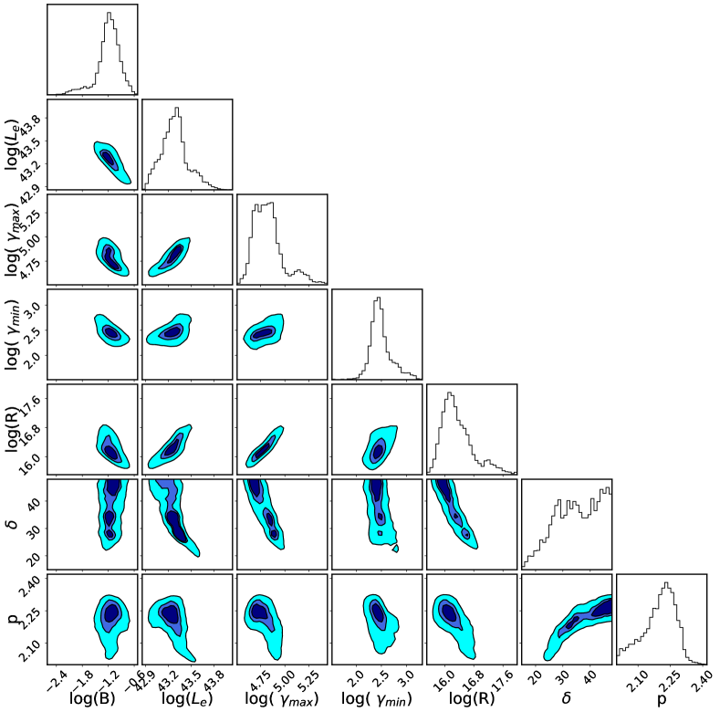
Figure 5: Parameter posterior distributions for Mrk 421 during the multi-wavelength campaign of 2009. The contours gives from outward to inward the 20%, 40%, and 75% confidence regions. Apart from the radius $R$, all parameters are well constrained.

Located at a redshift of $z=0.031$, Mrk 421 is one of the most extensively monitored blazars as it is the brightest blazar in the extragalactic X-ray sky. Owing to its proximity and brightness, the broadband emission features of Mrk 421 have been thoroughly investigated at all wavelengths from radio to VHE $\gamma$-rays. In 2009, a 4.5-month-long multi-wavelength campaign was conducted, yielding an unprecedented volume of simultaneous data (Abdo et al., 2011). The observed SED is presented in the left panel of Figure 3, where the set of data set is obtained from Abdo et al. (2011). We performed a fit to the SED, excluding data below $10^{11}$ Hz, as emission in the radio band can be self-absorbed, implying that it is dominated by the outer regions of the jet. The best-fit parameters are listed in the left column of Table 2. The left panel of Figure 3 displays the model uncertainty in grey and the best model, based on the best-fit parameters, in red. The posterior distribution functions are provided in Figure 5 in the appendix.

The model displayed in the left panel of Figure 3 accurately reproduces the observed data above 225 GHz. Given the current parameter set, self-absorption dominates below $1.3\times 10^{13}\,\text{Hz}$, making it impossible to model lower frequency data. The parameters we obtained are somewhat in agreement with the values determined by Abdo et al. (2011), who used a three-component power-law function to fit the broadband SED. In their model, the electron distribution between $\gamma_{\rm min}=8.0\times 10^{2}$ and $\gamma_{\rm brk,1}=5.0\times 10^{4}$ has an index of $2.2$, which is consistent with our estimated value of $p=2.16$ (for the errors see Table 2). In our approach the main difference is that we achieve an acceptable fit by assuming a single electron index for the injection, which is consistently evolved under the influence of radiation cooling. In our case, the synchrotron cooling would affect the spectrum at a frequency of $\approx 5.6\times 10^{17}$ Hz. This is above the maximum frequency defined by $\gamma_{\rm max}=7.37\times 10^{4}$ ($8.5\times 10^{16}$ Hz). Consequently, an electron spectrum with a power-law index of $p=2.16$?, above $\gamma_{\rm min}=2.10\times 10^{2}$ is sufficient to reproduce the observed spectrum. Our fit indicates that the magnetic field is around $B=6.70\times 10^{-2}$ G, which is in agreement with the value from Abdo et al. (2011) within the uncertainties. The dissipation radius we obtained, $R=2.96\times 10^{16}$ cm, is somewhat close to the value estimated in their model which was derived based on the variability time. We further find that the total luminosity of the electrons, $(L_{\rm e}=2.09\times 10^{43}\,{\rm erg\,s^{-1}}$, is of the same order of magnitude as the magnetic field luminosity $L_{\rm B}=1.19\times 10^{43}\,{\rm erg\,s^{-1}}$, calculated as $L_{B}=\pi cR^{2}\delta^{2}B^{2}/8\>\pi$. This suggests that the system is close to equipartition.

5.2 1ES 1959+650

Blazar 1ES 1959+650, at $z=0.048$, is another bright blazar known for frequent flaring across the optical, X-ray, and TeV bands. The X-ray and $\gamma$-ray (TeV) flares often occur simultaneously, although orphan $\gamma$-ray flares have also been observed. This suggest that the same population of electrons is responsible for emissions in both bands. The source was in an active state from April to November 2016, during which the MAGIC telescopes observed major VHE $\gamma$-ray flares on June 13 and 14, as well as July 1, 2016 (MAGIC Collaboration et al., 2020). The multi-wavelength campaigns conducted during these flaring periods also enabled the accumulation of data across lower-frequency bands, providing a comprehensive view of the flaring activities. In this study, we focus on modeling the flare observed on the 13^th of June 2016. We retrieved the data of the flare from MAGIC Collaboration et al. (2020). We note that the data are corrected for extragalactic background light (EBL) absorption. If it was not the case, our numerical model includes the possibility to incorporate EBL absorption, via the model of Domínguez et al. (2011).

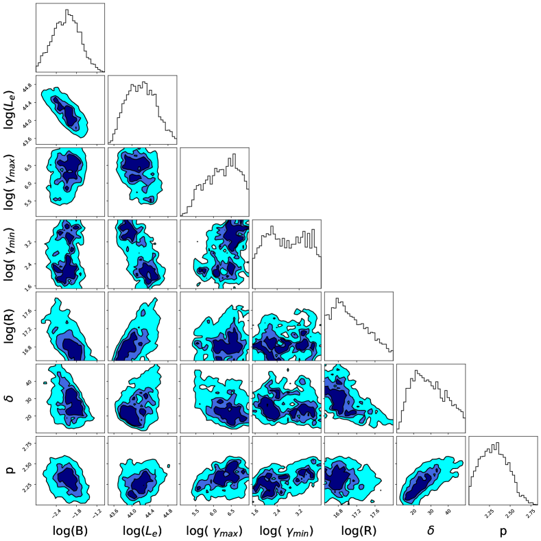
Figure 6: Parameter posterior distributions for 1ES 1959+650 without imposing a variability constraint. The magnetic field, the electron luminosity and the electron index are well constrained. In contrast, the other parameters remain somewhat unconstrained due to the high uncertainty in the position of peak energy of the synchrotron bump.

The fit to the data obtained during the flaring activity of 1ES 1959+650 is depicted in the right panel of Figure 3, and the corresponding parameter posterior distributions are provided in Figure 6. The best-fit parameters are summarized in Table 2. The data suggest that the synchrotron peak should occur at frequencies $\gtrsim 10^{20}$ Hz, enabling the X-ray data to constrain the power-law index of the electron injection function at $p=2.26$. In contrast to the case of Mrk 421 where the X-ray data define the high-energy tail of the synchrotron component, the value of the parameter $\gamma_{\rm cut}=2.57\times 10^{6}$ is not well-constrained in this case. It is determined solely by the last data of the MAGIC spectrum, which have a large uncertainty. The interpretation of the parameter is also difficult because of the EBL effect at these high frequencies. The fit to our model constrains the magnetic field to be $2.4\times 10^{-2}$G and the Doppler boost $\delta$ to be $22.49$. The parameters $p$, $\gamma_{\rm cut}$, and $\delta$ are similar to those proposed by MAGIC Collaboration et al. (2020), but the magnetic field and the radius $R$ differ significantly.

The dissipation radius $R=6.69\times 10^{16}$cm is rather large and the value of the Doppler factor is average, $\delta=22.49$, which leads to an estimated variability time of $t_{\rm var}\sim 10^{5}$s, which is much longer than the reported variability time of approximately 36 min (MAGIC Collaboration et al., 2020). Although our fitting procedure generally treats the radius $R$ and $\delta$ as independent variables, we can easily couple these parameters by specifying the variability timescale and removing one of them from the model parameter. To illustrate this approach, we set the radius to be $R=c\delta t_{\rm var}$ and retain $\delta$ as a free parameter. In order to not jump outside of the parameter range, the bounds on $\delta$ are changed to $\delta_{\rm min}={\rm max}(3,R_{\rm min}/(ct_{\rm var}))$ and $\delta_{\rm max}={\rm min}(50,R_{\rm max}/(ct_{\rm var}))$.

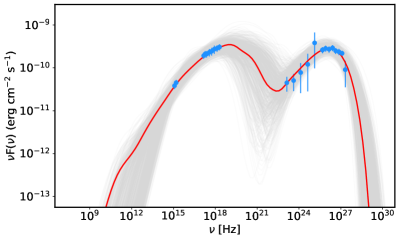
Figure 4: The same SED of 1ES 1959+650 as presented in Fig. 3, but fitted with a model where $R$ is constrained by a variability of 35 minutes.

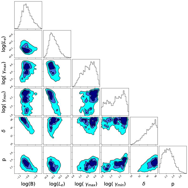
Figure 7: Parameter posterior distributions for 1ES 1959+650 assuming a variability time of 35 minutes to link the radius and the Doppler boost. Additionally, there exists a large uncertainty on the minimum electron Lorentz factor $\gamma_{\rm min}$

The fit results are illustrated in Figure 4, while the parameter posterior distributions are presented in Figure 7. The best-fit parameters are listed in the rightmost column of Table 2. A significant difference is observed in the value of the Doppler boost parameter, $\delta$, which has shifted to larger values, compared to $\delta\approx 22.49$ in the previous scenario. This indicates that the compact emission region is moving at a higher velocity. Additionally, the magnetic field density in this case is larger — $B\sim 0.24$G as opposed to $B\sim 0.02$G in the previous case — which influences the electron cooling process. In the first case, synchrotron cooling is inefficient for all electrons. However, in the second case, the synchrotron cooling is efficient for the highest energy electrons, and a cooling break occurs at $\sim 2\times 10^{17}$ Hz, resulting in the X-ray emission to be produced by cooled electrons.

6 Conclusion

In this work, we presented a new approach to fit multi-wavelength SEDs of blazars with numerically intensive models. Indeed, there is a clear gap between the computational resources needed for each model evaluation and the analysis, fitting, and detailed interpretation of multi-wavelength (and soon, multi-messenger) data for blazars. To bridge these two aspects of blazar SEDs analysis, we developed a neural network that can be trained on different computationally demanding numerical models. In this study, the CNN is trained on a large set of SSC spectra generated by SOPRANO, taking into account all relevant cooling processes and the pair creation process. Our surrogate model achieves high accuracy, is computed in a relatively short time $\sim$ms, includes the self-consistent cooling of the electron, and enables on-the-fly fits to data. We demonstrate the performance of the CNN by fitting the multi-wavelength observations of two BL Lac objects, namely Mrk 421 and 1ES 1959+650, thereby constraining the parameters of the SSC model and obtaining their posterior distributions.

The significant advantage of the method proposed in this work is its computational speed; the model performs fast independently of of the considered physical processes and is expected to do so when hadronic processes will be included. However, a key limitation of this approach is the initial requirement for the substantial computational resources to generate the spectra needed for training the CNN. Once this initial step is completed, our methodology enables efficient and straightforward analysis of blazar SEDs. The low computational cost of the model evaluation via the CNN offers the advantage of enabling more sophisticated data fitting techniques. In future works, this efficiency will permit us to allocate computational resources for model forward-folding. Specifically, instead of using pre-analyzed data, we plan to utilize raw observational data in conjunction with the response functions of various instruments, such as Swift-XRT and Fermi-LAT. This integration will be facilitated through the use of 3ML (Vianello et al., 2015), a framework specifically designed to combine analyses from different instruments across energy bands into a unified, coherent picture.

In this study, we trained the first convolutional neural network to accurately model the radiative signatures associated with the SSC model. This approach provides a novel framework for fitting the SED of blazars, and we intend to further apply it to other models of blazar SEDs. Specifically, we plan to implement additional computationally intensive models based on external Compton and hadronic scenarios, for which the CNN will be trained. This set of models will facilitate the interpretation of a large variety of blazar SEDs, spanning various wavelengths, time periods, and sources.

We believe that the approach outlined in this paper has the potential to provide significant advances of our understanding of blazars by enabling the fitting of self-consistent models to their SEDs. To facilitate broader analysis and interpretation, the model developed here will be made publicly available on the Markarian Multiwavelength Datacenter (mmdc). Users will be able to interact with an interface to reproduce single snapshot SEDs by specifying model parameters. Additionally, users will be able to perform fits after uploading their data (if necessary), which will provide them with the parameters that best describe the observed data, along with their posterior distributions. It should be noted that, as of the current time, this will be the only public tool available for performing fits with self-consistent model of blazar SEDs.

Not only the CNN and the associated methodology could be applied to several model of blazar as demonstrated here, but we believe that it is sufficiently general and robust to also be used in spectral and temporal analysis of gamma-ray bursts prompt and afterglow phase, multi-wavelength temporal evolution of kilonovae (e.g. Boersma & van Leeuwen, 2023), and for the spectral interpretation of X-ray binaries.

In summary, this study represents a pioneering effort in employing convolutional neural networks for the efficient and accurate modeling of blazar SEDs. We have introduced a flexible and efficient methodology for self-consistent blazar modeling, which holds the potential for deepening our understanding of blazar physics. With the tool made publicly available through the Markarian Multiwavelength Data center, researchers will be able to perform state-of-the-art, self-consistent analyses of multi-wavelength—and soon, multi-messenger-data from blazar observations.

Data availability

All the observational data used in this paper is public. The convolutional neural network used to fit the SEDs can be shared on a reasonable request to the corresponding author. In addition, it is publicly available through the Markarian Multiwavelength Datacenter (http://www.mmdc.am).

Appendix A Parameter posterior for Mrk 421 and 1ES 1959+650

.

References

- Abdo et al. (2011) Abdo A. A., et al., 2011, ApJ, 736, 131
- Abe et al. (2023) Abe H., et al., 2023, ApJS, 266, 37
- Ackermann et al. (2017) Ackermann M., et al., 2017, ApJ, 837, L5
- Ahnen et al. (2017) Ahnen M. L., et al., 2017, A&A, 603, A31
- Ansoldi et al. (2018) Ansoldi S., et al., 2018, ApJ, 863, L10
- Beckmann & Shrader (2012) Beckmann V., Shrader C. R., 2012, Active Galactic Nuclei
- Blandford & Rees (1978) Blandford R. D., Rees M. J., 1978, in Wolfe A. M., ed., BL Lac Objects. pp 328–341
- Błażejowski et al. (2000) Błażejowski M., Sikora M., Moderski R., Madejski G. M., 2000, ApJ, 545, 107
- Bloom & Marscher (1996) Bloom S. D., Marscher A. P., 1996, ApJ, 461, 657
- Boersma & van Leeuwen (2023) Boersma O. M., van Leeuwen J., 2023, PASA, 40, e030
- Böttcher et al. (2013) Böttcher M., Reimer A., Sweeney K., Prakash A., 2013, ApJ, 768, 54
- Burgess (2023) Burgess J. M., 2023, The Journal of Open Source Software, 8, 4969
- Cerruti et al. (2015) Cerruti M., Zech A., Boisson C., Inoue S., 2015, MNRAS, 448, 910
- Cerruti et al. (2019) Cerruti M., Zech A., Boisson C., Emery G., Inoue S., Lenain J.-P., 2019, MNRAS, 483, L12
- Dermer & Schlickeiser (1994) Dermer C. D., Schlickeiser R., 1994, ApJS, 90, 945
- Dermer et al. (1992) Dermer C. D., Schlickeiser R., Mastichiadis A., 1992, A&A, 256, L27
- Dermer et al. (2009) Dermer C. D., Finke J. D., Krug H., Böttcher M., 2009, ApJ, 692, 32
- Domínguez et al. (2011) Domínguez A., et al., 2011, MNRAS, 410, 2556
- Feroz et al. (2009) Feroz F., Hobson M. P., Bridges M., 2009, MNRAS, 398, 1601
- Finke et al. (2008) Finke J. D., Dermer C. D., Böttcher M., 2008, ApJ, 686, 181
- Gao et al. (2017) Gao S., Pohl M., Winter W., 2017, ApJ, 843, 109
- Gao et al. (2019) Gao S., Fedynitch A., Winter W., Pohl M., 2019, Nature Astronomy, 3, 88
- Gasparyan et al. (2022) Gasparyan S., Bégué D., Sahakyan N., 2022, MNRAS, 509, 2102
- Ghisellini & Tavecchio (2009) Ghisellini G., Tavecchio F., 2009, MNRAS, 397, 985
- Ghisellini et al. (1985) Ghisellini G., Maraschi L., Treves A., 1985, A&A, 146, 204
- IceCube Collaboration et al. (2018a) IceCube Collaboration et al., 2018a, Science, 361, 147
- IceCube Collaboration et al. (2018b) IceCube Collaboration et al., 2018b, Science, 361, eaat1378
- Kamath (2022) Kamath C., 2022, Machine Learning with Applications, 9, 100373
- Keivani et al. (2018a) Keivani A., et al., 2018a, ApJ, 864, 84
- Keivani et al. (2018b) Keivani A., et al., 2018b, ApJ, 864, 84
- Kirk et al. (2000) Kirk J. G., Guthmann A. W., Gallant Y. A., Achterberg A., 2000, ApJ, 542, 235
- MAGIC Collaboration et al. (2020) MAGIC Collaboration et al., 2020, A&A, 638, A14
- Mannheim (1993) Mannheim K., 1993, A&A, 269, 67
- Mannheim & Biermann (1989) Mannheim K., Biermann P. L., 1989, A&A, 221, 211
- Maraschi et al. (1992) Maraschi L., Ghisellini G., Celotti A., 1992, ApJ, 397, L5
- Mastichiadis & Kirk (1995) Mastichiadis A., Kirk J. G., 1995, A&A, 295, 613
- McKay et al. (2000) McKay M. D., Beckman R. J., Conover W. J., 2000, Technometrics, 42, 55
- Mücke & Protheroe (2001) Mücke A., Protheroe R. J., 2001, Astroparticle Physics, 15, 121
- Mücke et al. (2003) Mücke A., Protheroe R. J., Engel R., Rachen J. P., Stanev T., 2003, Astroparticle Physics, 18, 593
- Murase et al. (2018) Murase K., Oikonomou F., Petropoulou M., 2018, ApJ, 865, 124
- Nigro et al. (2022) Nigro C., Sitarek J., Gliwny P., Sanchez D., Tramacere A., Craig M., 2022, A&A, 660, A18
- Padovani et al. (2017) Padovani P., et al., 2017, A&A Rev., 25, 2
- Padovani et al. (2018) Padovani P., Giommi P., Resconi E., Glauch T., Arsioli B., Sahakyan N., Huber M., 2018, MNRAS, 480, 192
- Petropoulou & Mastichiadis (2015) Petropoulou M., Mastichiadis A., 2015, MNRAS, 447, 36
- Petropoulou et al. (2015) Petropoulou M., Dimitrakoudis S., Padovani P., Mastichiadis A., Resconi E., 2015, MNRAS, 448, 2412
- Rau et al. (2012) Rau A., et al., 2012, A&A, 538, A26
- Righi et al. (2019) Righi C., Tavecchio F., Pacciani L., 2019, MNRAS, 484, 2067
- Rodrigues et al. (2023) Rodrigues X., Paliya V. S., Garrappa S., Omeliukh A., Franckowiak A., Winter W., 2023, arXiv e-prints, p. arXiv:2307.13024
- Sahakyan (2018) Sahakyan N., 2018, ApJ, 866, 109
- Sahakyan (2019) Sahakyan N., 2019, A&A, 622, A144
- Sahakyan (2021) Sahakyan N., 2021, MNRAS, 504, 5074
- Sahakyan & Giommi (2022) Sahakyan N., Giommi P., 2022, MNRAS, 513, 4645
- Sahakyan et al. (2020) Sahakyan N., Israyelyan D., Harutyunyan G., Khachatryan M., Gasparyan S., 2020, MNRAS, 498, 2594
- Sahakyan et al. (2022) Sahakyan N., Israyelyan D., Harutyunyan G., Gasparyan S., Vardanyan V., Khachatryan M., 2022, MNRAS, 517, 2757
- Sahakyan et al. (2023a) Sahakyan N., Giommi P., Padovani P., Petropoulou M., Bégué D., Boccardi B., Gasparyan S., 2023a, MNRAS, 519, 1396
- Sahakyan et al. (2023b) Sahakyan N., Harutyunyan G., Israyelyan D., 2023b, MNRAS, 521, 1013
- Sikora et al. (1994) Sikora M., Begelman M. C., Rees M. J., 1994, ApJ, 421, 153
- Sikora et al. (2009) Sikora M., Stawarz Ł., Moderski R., Nalewajko K., Madejski G. M., 2009, ApJ, 704, 38
- Sironi & Spitkovsky (2011) Sironi L., Spitkovsky A., 2011, ApJ, 726, 75
- Stathopoulos et al. (2022) Stathopoulos S. I., Petropoulou M., Giommi P., Vasilopoulos G., Padovani P., Mastichiadis A., 2022, MNRAS, 510, 4063
- Stathopoulos et al. (2023) Stathopoulos S. I., Petropoulou M., Vasilopoulos G., Mastichiadis A., 2023, arXiv e-prints, p. arXiv:2308.06174
- Tavecchio et al. (1998) Tavecchio F., Maraschi L., Ghisellini G., 1998, ApJ, 509, 608
- Tramacere (2020) Tramacere A., 2020, JetSeT: Numerical modeling and SED fitting tool for relativistic jets, Astrophysics Source Code Library, record ascl:2009.001 (ascl:2009.001)
- Tramacere et al. (2009) Tramacere A., Giommi P., Perri M., Verrecchia F., Tosti G., 2009, A&A, 501, 879
- Tramacere et al. (2011) Tramacere A., Massaro E., Taylor A. M., 2011, ApJ, 739, 66
- Urry & Padovani (1995) Urry C. M., Padovani P., 1995, PASP, 107, 803
- Uzdensky (2022) Uzdensky D. A., 2022, Journal of Plasma Physics, 88, 905880114
- Viana (2016) Viana F. A., 2016, Quality and reliability engineering international, 32, 1975
- Vianello et al. (2015) Vianello G., et al., 2015, preprint, (arXiv:1507.08343)
- Zabalza (2015) Zabalza V., 2015, Proc. of International Cosmic Ray Conference 2015, p. 922